the Creative Commons Attribution 4.0 License.
the Creative Commons Attribution 4.0 License.
 | 27 Jan 2020
Six global biomass burning emission datasets: intercomparison and application in one global aerosol model
Charles Ichoku
Mian Chin
Huisheng Bian
Anton Darmenov
Peter Colarco
Luke Ellison
Tom Kucsera
Arlindo da Silva
Tomohiro Oda
Ge Cui
Aerosols from biomass burning (BB) emissions are poorly constrained in global and regional models, resulting in a high level of uncertainty in understanding their impacts. In this study, we compared six BB aerosol emission datasets for 2008 globally as well as in 14 regions. The six BB emission datasets are (1) GFED3.1 (Global Fire Emissions Database version 3.1), (2) GFED4s (GFED version 4 with small fires), (3) FINN1.5 (FIre INventory from NCAR version 1.5), (4) GFAS1.2 (Global Fire Assimilation System version 1.2), (5) FEER1.0 (Fire Energetics and Emissions Research version 1.0), and (6) QFED2.4 (Quick Fire Emissions Dataset version 2.4). The global total emission amounts from these six BB emission datasets differed by a factor of 3.8, ranging from 13.76 to 51.93 Tg for organic carbon and from 1.65 to 5.54 Tg for black carbon. In most of the regions, QFED2.4 and FEER1.0, which are based on satellite observations of fire radiative power (FRP) and constrained by aerosol optical depth (AOD) data from the Moderate Resolution Imaging Spectroradiometer (MODIS), yielded higher BB aerosol emissions than the rest by a factor of 2–4. By comparison, the BB aerosol emissions estimated from GFED4s and GFED3.1, which are based on satellite burned-area data, without AOD constraints, were at the low end of the range. In order to examine the sensitivity of model-simulated AOD to the different BB emission datasets, we ingested these six BB emission datasets separately into the same global model, the NASA Goddard Earth Observing System (GEOS) model, and compared the simulated AOD with observed AOD from the AErosol RObotic NETwork (AERONET) and the Multiangle Imaging SpectroRadiometer (MISR) in the 14 regions during 2008. In Southern Hemisphere Africa (SHAF) and South America (SHSA), where aerosols tend to be clearly dominated by smoke in September, the simulated AOD values were underestimated in almost all experiments compared to MISR, except for the QFED2.4 run in SHSA. The model-simulated AOD values based on FEER1.0 and QFED2.4 were the closest to the corresponding AERONET data, being, respectively, about 73 % and 100 % of the AERONET observed AOD at Alta Floresta in SHSA and about 49 % and 46 % at Mongu in SHAF. The simulated AOD based on the other four BB emission datasets accounted for only ∼50 % of the AERONET AOD at Alta Floresta and ∼20 % at Mongu. Overall, during the biomass burning peak seasons, at most of the selected AERONET sites in each region, the AOD values simulated with QFED2.4 were the highest and closest to AERONET and MISR observations, followed closely by FEER1.0. However, the QFED2.4 run tends to overestimate AOD in the region of SHSA, and the QFED2.4 BB emission dataset is tuned with the GEOS model. In contrast, the FEER1.0 BB emission dataset is derived in a more model-independent fashion and is more physically based since its emission coefficients are independently derived at each grid box. Therefore, we recommend the FEER1.0 BB emission dataset for aerosol-focused hindcast experiments in the two biomass-burning-dominated regions in the Southern Hemisphere, SHAF, and SHSA (as well as in other regions but with lower confidence). The differences between these six BB emission datasets are attributable to the approaches and input data used to derive BB emissions, such as whether AOD from satellite observations is used as a constraint, whether the approaches to parameterize the fire activities are based on burned area, FRP, or active fire count, and which set of emission factors is chosen.
- Article
(10843 KB) -
Supplement
(1402 KB) - BibTeX
- EndNote


Biomass burning (BB) is estimated to contribute about 62 % of the global particulate organic carbon (OC) and 27 % of black carbon (BC) emissions annually (Wiedinmyer et al., 2011). Therefore, biomass burning emissions significantly affect air quality by acting as a major source of particulate matter (PM) and the climate system by modulating solar radiation and cloud properties. For instance, a number of studies have revealed that wildfire smoke exposure is harmful to human health by causing general respiratory morbidity and exacerbating asthma, because approximately 80 %–90 % of the smoke particles produced by biomass burning fall within the PM2.5 size range (PM with aerodynamic diameter less than 2.5 µm) (Reid et al., 2005, 2016). Moreover, biomass burning emissions have been shown to impact the atmospheric composition in different regions, such as South America (Reddington et al., 2016), Central America (Wang et al., 2006), the sub-Saharan African region (Yang et al., 2013), Southeast Asia (Wang et al., 2013; Pan et al., 2018), China (Zhu et al., 2017), and the western Arctic (Bian et al., 2013). Additionally, BB-produced aerosols can also directly impact the upper troposphere and lower stratosphere via extreme pyro-convection events associated with intense wildfires that generate the storms injecting smoke particles and trace gases to high altitudes (e.g., Peterson et al., 2018). Therefore, emissions from biomass burning constitute a significant component of the climate system and are crucial inputs required by chemical transport and atmospheric circulation models used to simulate the atmospheric composition, radiation, and circulation processes involved in air-quality and climate-impact studies (e.g., van Marle et al., 2017).
With the advent of satellite remote sensing of active fires and burned areas in the last couple of decades, a number of global BB emission datasets based on these observations have become available (e.g., Ichoku et al., 2012). Six such major BB datasets will be compared in this study, including three datasets based on burned area approaches, namely the Fire INventory from NCAR (FINN; Wiedinmyer et al., 2011), two versions of the Global Fire Emissions Database (GFED; van der Werf et al., 2006, 2010, 2017), and three datasets based on fire radiative power (FRP) approaches, namely the Global Fire Assimilation System (GFAS; Kaiser et al., 2012) developed in the European Centre for Medium-Range Weather Forecasts (ECMWF) and two National Aeronautics and Space Administration (NASA) products, i.e., the Fire Energetics and Emissions Research algorithm (FEER; Ichoku and Ellison, 2014) and the Quick Fire Emissions Dataset (QFED; Darmenov and da Silva, 2015).
Although much progress has been made over the last couple of decades in improving the quality of BB emission datasets, for example, by incorporating more recent satellite measurements with better calibration and spatial resolution (e.g., van der Werf et al., 2010, 2017), biomass burning aerosol emissions still have large uncertainty and thus are still poorly constrained in models at global and regional levels (e.g., Liousse et al., 2010; Kaiser et al., 2012; Petrenko et al., 2012, 2017; Bond et al., 2013; Zhang et al., 2014; Pan et al., 2015; Ichoku et al., 2016a; Reddington et al., 2016; Pereira et al., 2016). Specifically, large uncertainty exists in the description of the magnitude, patterns, and drivers of wildfires and types of biomass burning (e.g., Hyer et al., 2011). For instance, a global enhancement of particulate matter BB emission by a factor of 3.4 was recommended for GFAS by Kaiser et al. (2012) to match the corresponding observed aerosol loading. Andreae (2019) commented that
in contrast to gaseous compounds, which are chemically well defined, aerosols are complex and variable mixtures of organic and inorganic species and comprise particles across a wide range of sizes. This affects in particular the measurements of organic aerosol, black/elemental carbon, and size fractionated aerosol mass.
A recent analysis with multiple models has been conducted under the auspices of the Aerosol Comparisons between Observations and Models (AeroCom) Phase III biomass burning emission experiments using the GFED version 3.1 (GFED3.1) emission dataset as input to several models (hereinafter “the AeroCom multi-model study”, https://wiki.met.no/aerocom/phase3-experiments, last access: 17 January 2020) (Mariya Petrenko, personal communication, 2019). The AeroCom multi-model study concluded that the modeled aerosol optical depth (AOD) from different models exhibits large diversity in most regions; i.e., some models overestimate while other models underestimate. However, over two major biomass-burning-dominated regions, South America and Southern Hemisphere Africa, all models consistently underestimate AOD. That result suggests that the underestimation of AOD in these two regions was more likely attributable to the GFED3.1 biomass burning emission dataset rather than the model configurations.
Our study aims to explore multiple BB emission datasets, including GFED3.1, GFED version 4 with small fires (GFED4s), FINN version 1.5, GFAS version 1.2, QFED version 2.4, and FEER version 1.0, in order to investigate the discrepancies between these six BB emission datasets by comparing them at both regional and global levels. Such a comparative evaluation of BB emission datasets would show the differences between them as well as how these differences propagate through the physical processes of related aerosols in models, e.g., dry and wet deposition, transport, atmospheric abundance, and the resulting AOD. Our study is expected to provide further insight into the development of possible mitigation for the current large uncertainties in BB emissions. Similar comparative studies of multiple BB aerosol emission datasets were previously conducted at regional scales, e.g., by Zhang et al. (2014) in the northern sub-Saharan African region, Pereira et al. (2016) and Reddington et al. (2019) in South America, and Reddington et al. (2016) in the entire tropical region. The current study not only provides a global assessment and analysis of these six BB emission datasets to provide a worldwide perspective, but also examines their performance within 14 regions (Fig. 1) which were previously defined for a series of GFED-based studies (e.g., van der Werf et al., 2006, 2010, 2017).
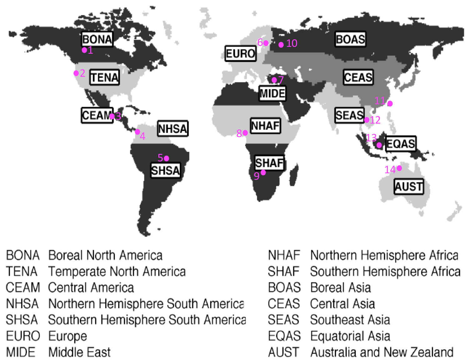
Figure 1Map showing the 14 regions used in this study, following GFED regionalization defined by Giglio et al. (2006) and van der Werf et al. (2006, 2017). The 14 AERONET sites selected for detailed analysis in the respective regions are represented by the numbered magenta dots. These AERONET sites and the included data (years in parentheses) for calculating aerosol climatology are 1 – Fort McMurray (2005–2018), 2 – Monterey (2002–2018), 3 – Tuxtla Gutiérrez (2005–2010), 4 – Medellín (2012–2016), 5 – Alta Floresta (1993–2018), 6 – Tõravere (2002–2017), 7 – IMS METU ERDEMLI (1999–2017), 8 – Ilorin (1998–2018), 9 – Mongu (1997–2010), 10 – Moscow MSU MO (2001–2017), 11 – EPA NCU (2004–2018), 12 – Chiang Mai Met Sta (2007–2017), 13 – Palangkaraya (2012–2017), and 14 – Lake Argyle (2001–2017).
In the rest of this paper, we first describe these six BB emission datasets, the GEOS model configuration and experimental designs, and observations in Sect. 2, and then we show comparisons of the biomass burning emission datasets and the resulting model-simulated AOD in Sect. 3. We discuss possible attributions of the differences between the six BB emission datasets to the sources of uncertainty associated with the biomass burning emissions and the aerosol modeling in Sect. 4. Conclusions and recommendations are presented in Sect. 5.
2.1 Six BB emission datasets
General information about each of the six biomass burning emission datasets investigated in this study, namely GFED3.1, GFED4s, FINN1.5, GFAS1.2, FEER1.0, and QFED2.4, is given below. Their main attributes, such as their spatial and temporal resolutions, the methods used to estimate burned area (where applicable), the method to derive emission coefficients (where applicable), and the references for the emission factors, are compared in Table 1. Overall, all datasets provide daily global biomass burning emissions since at least 2003.
Table 1Summary of six biomass burning emission datasets during the MODIS era (i.e., 2000–present).
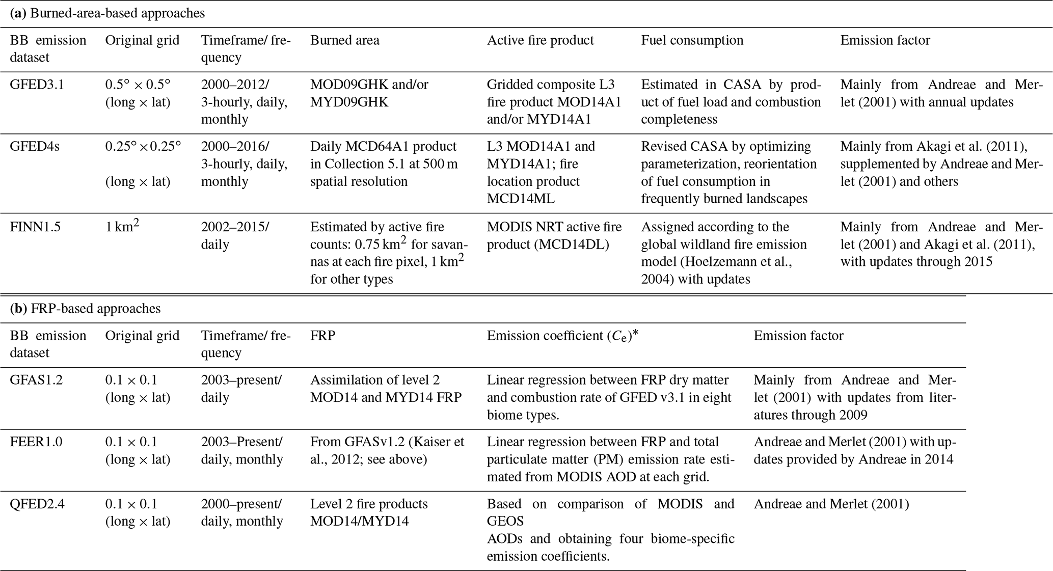
CASA: Carnegie-Ames-Stanford Approach biogeochemical. ∗ Conversion factor for the case of GFAS.
2.1.1 GFED3.1
The total dry matter consumed by biomass burning in GFED3.1 (van der Werf et al., 2010) is estimated by the multiplication of the MODIS burned area product at 500 m spatial resolution (Giglio et al., 2010, for the MODIS era) and fuel consumption per unit burned area, the latter being the product of the fuel loads per unit area and combustion completeness. This estimation is conducted using the Carnegie–Ames–Stanford approach (CASA) biogeochemical modeling framework that provides estimates of biomass in various carbon “pools” including leaves, grasses, stems, coarse woody debris, and litter. Fuel loads in CASA are estimated according to carbon input information on vegetation productivity, and carbon outputs through heterotrophic respiration, herbivory, fires, and tree mortality (Giglio et al., 2010; van der Werf et al., 2010). Then, the biomass burning emission of a given species is calculated by multiplying the dry matter with an emission factor of that species (EF, in grams of species per kilogram of dry matter burned). The EF used in GFED3.1 (and most of the other datasets) is mainly chosen from Andreae and Merlet (2001) and/or Akagi et al. (2011), but may also be obtained from various other sources. The GFED3.1 dataset can be accessed through the following link: https://daac.ornl.gov/VEGETATION/guides/global_fire_emissions_v3.1.html (last access: 17 January 2020).
2.1.2 GFED4s
Compared to GFED3.1, the latest GFED version, GFED4s, has a few significant upgrades as described in detail by van der Werf et al. (2017), including (1) additional burned area associated with small fires which were previously omitted by the burned area product but now are compensated for by including the active fires to augment the burned area product MCD64A1 (Giglio et al., 2013; Randerson et al., 2012); (2) a revised fuel consumption parameterization optimized using field observations (e.g., van Leeuwen et al., 2014); and (3) further dividing forest into temperate and boreal forest ecosystems and applying different sets of emission factors. Among the existing BB emission datasets, GFED4s has hitherto been the most widely used by modeling communities, such as the Coupled Model Intercomparison Project Phase 6 (CMIP6; Van Marle et al., 2017) and AeroCom phase III experiments (https://wiki.met.no/aerocom/phase3-experiments). The link to the GFED4s dataset is http://www.globalfiredata.org (last access: 17 January 2020).
2.1.3 FINN1.5
The FINN1.5 biomass burning emission dataset is developed from its previous version FINN1 (Wiedinmyer et al., 2011) with several updates. It uses satellite observation of active fire (with a confidence level greater than 20 %) and land cover from the MODIS instruments on board the NASA Terra and Aqua polar-orbiting satellites, together with the estimated fuel consumption to derive biomass burning emissions. The burned area in each active fire pixel is assumed as 1 km2, except for grasslands and savannas where it is assigned a value of 0.75 km2. The fuel consumption at each fire pixel is estimated according to its generic land use–land cover type (LULC) which is assigned using values updated from Table 2 of Hoelzemann et al. (2004) in the various world regions based on Global Wildland Fire Emission Model (GWEM). With the estimated burned area, fuel consumption, and EF of individual species, the daily global open biomass burning emissions of each species are then calculated at a 1 km spatial resolution. The FINN1.5 emissions dataset is archived at http://bai.acom.ucar.edu/Data/fire/ (last access: 17 January 2020).
2.1.4 GFAS1.2
The GFAS (Kaiser et al., 2012) estimates dry matter combustion rate by multiplying FRP and biome-specific conversion factors (units: kilograms of dry matter per megajoule). The global distribution of FRP observations is obtained from the MODIS instruments on board the Terra and Aqua satellites and are then assimilated into the GFAS system. The gaps in FRP observations, which are mostly due to cloud cover and spurious FRP observations of volcanoes, gas flares, and other industrial activity, are corrected or filtered in the GFAS system. Eight biome-specific conversion factors are calculated by linear regressions between the GFAS FRP and the dry matter combustion rate of GFED3.1 in each biome (see Table 2 and Fig. 3 in Kaiser et al., 2012). The biomass burning emission of a given species is calculated by multiplying the dry matter with an emission factor of that species. More information on the latest GFAS product can be found at https://apps.ecmwf.int/datasets/data/cams-gfas/ (last access: 17 January 2020).
2.1.5 FEER1.0
The FEER1.0 (Ichoku and Ellison, 2014) multiplies its emission coefficients Ce with MODIS FRP data that have been preprocessed and gridded in the GFAS1.2 analysis system (Kaiser et al., 2012) to derive biomass burning aerosol emission rates. The Ce in FEER1.0 for smoke aerosol total particulate matter (TPM) was derived through zero-intercept regression of the emission rate of smoke aerosol (i.e., Rsa) against the corresponding FRP (Ichoku and Kaufman, 2005; Ichoku and Ellison, 2014) at pixel level within each grid. Ce corresponds to the slope of the linear regression fitting. In the FEER methodology, Rsa is estimated through a spatiotemporal analysis of MODIS AOD data along with wind fields from the NASA Modern-Era Retrospective Analysis for Research and Applications (MERRA) reanalysis dataset (Rienecker et al., 2011). The smoke aerosol Ce in FEER1.0 is available at spatial resolution global grid and covers most of the land areas where fires have been detected by MODIS at least 30 times during the period 2003–2010 (Ichoku and Ellison, 2014) to ensure statistical representativeness. In the current version of the FEER1.0 emission dataset, Ce values for other smoke constituents, say OC, at each grid cell are obtained by scaling the Ce of smoke aerosol according to the ratio of their emission factors, such as EFoc to EFsa (i.e., ratio of emission factor for OC to that for total smoke aerosol). The FEER1.0 dataset is available at http://feer.gsfc.nasa.gov/data/emissions/ (last access: 17 January 2020).
2.1.6 QFED2.4
In QFED (Darmenov and da Silva, 2015) biomass burning aerosol emissions are estimated using gridded MODIS Terra and MODIS Aqua FRP and emission coefficients Ce, which are the product of a constant value C0 (1.37 kg MJ−1, reported by Kaiser et al., 2009), satellite factor, and biome-specific scaling factor. The scaling factors used in QFED2.4, the version applied in this study, were obtained by comparing AOD from the Goddard Earth Observing System model (GEOS) and MODIS aerosol product in multiple sub-regions (Fig. 4 in Darmenov and da Silva, 2015). These scaling factors were further reduced to four values representative of fires in savanna, grassland, tropical forests, and extratropical forests – 1.8, 1.8, 2.5, and 4.5, respectively. The QFED2.4 used a sequential model with temporally damped emissions to estimate the emissions in cloudy areas. QFED is the standard fire emissions dataset in the near-real-time GEOS data assimilation system and the MERRA-2 reanalysis (Randles et al., 2017). QFED2.4 emissions are available from https://portal.nccs.nasa.gov/datashare/iesa/aerosol/emissions/QFED/v2.4r6/ (last access: 17 January 2020).
2.2 Application of the BB emission datasets in the NASA GEOS model
2.2.1 Description of the NASA GEOS model
The GEOS model consists of an atmospheric general circulation model, a catchment-based land surface model, and an ocean model, all coupled together using the Earth System Modeling Framework (ESMF; Rienecker et al., 2011; Molod et al., 2015). Within the GEOS model architecture, several interactively coupled atmospheric constituent modules have been incorporated, including an aerosol and carbon monoxide (CO) module based on the Goddard Chemistry Aerosol Radiation and Transport model (GOCART; Chin et al., 2000, 2002, 2009, 2014; Colarco et al., 2010; Bian et al., 2010) and a radiation module from the Goddard radiative transfer model (Chou and Suarez, 1999; Chou et al., 2001). The GOCART module used in this study includes representations of dust, sea salt, sulfate, nitrate, and black and organic carbon aerosol species. A conversion factor of 1.4 is used to scale organic carbon mass to organic aerosol (OA), which is on the low end of current estimates (Simon and Bhave, 2012). More discussion on this conversion factor can be referred to in Sect. 4.3.
In this study the GEOS model (Heracles-5.2 version) was run globally on a cubed-sphere horizontal grid (c180, ∼ 50 km resolution) and with 72 vertical hybrid-sigma levels extending from the surface to ∼85 km for the year 2008. The reason we chose 2008 is because it is the year assigned as a benchmark year by the AeroCom community with which this study is associated; it is also because the AeroCom multi-model study of biomass burning led by Petrenko (mentioned in the introduction) also chose 2008 as a focus year. As such, the results from these two studies can be intercompared to draw some synthesized conclusions. In addition, 2008 was chosen because it is a neutral El Niño–Southern Oscillation (ENSO) year, which represents normal burning conditions. The model was run in a “replay” mode, where the winds, pressure, moisture, and temperature are constrained by the MERRA-2 reanalysis meteorological data (Gelaro et al., 2017), a configuration that allows a similar simulation of real events as in a traditional offline chemistry transport model (CTM) but exercises the full model physics for radiation, for example, and moist physics processes. We used the HTAP2 anthropogenic emissions (Janssens-Maenhout et al., 2015) that provide high-spatial-resolution monthly emissions. The BB emissions are uniformly distributed within the boundary layer without considering the specific injection height of each plume. All six BB emissions are daily emissions with the diurnal cycle prescribed in the model: the maximum is around local noon, which is more prominent in the tropics, and is gradually weakened in the extra-tropics (Randles et al., 2017). The natural aerosols are either generated by the model itself (i.e., wind-blown dust and sea salt) or come from prescribed emission files (i.e., volcanic and biogenic aerosols).
2.2.2 Experiment design
In order to investigate the sensitivity of the modeled AOD to different BB emission datasets, seven experiments were conducted with the GEOS model, differing only in the source of biomass burning emissions. The first six runs are GFED3.1, GFED4s, FINN1.5, GFAS1.2, FEER1.0, and QFED2.4, using the corresponding biomass burning datasets described above in Sect. 2.1. A seventh run is called “NOBB,” where the model is run without including biomass burning emissions.
2.3 AOD observations
2.3.1 MISR retrievals
We evaluated the simulated monthly AOD at 550 nm with the monthly level 3 total AOD data at the 558 nm wavelength from the Multiangle Imaging SpectroRadiometer sensor on board the EOS Terra satellite (Kalashnikova and Kahn, 2006; Kahn et al., 2010). We used MISR version 23 data products (MISR v23, with filename tagged as F15_0032) in half-degrees, which can be downloaded from the website https://eosweb.larc.nasa.gov/project/misr/mil3mae_table (last access: 17 January 2020).
2.3.2 AERONET sites
We also evaluated the modeled 3-hourly and monthly AOD at 550 nm and Ångström exponent (AE, 440–870 nm) with corresponding measurements from the ground-based AErosol RObotic NETwork (AERONET; Holben et al., 1998) sites situated in biomass burning source regions. AERONET Version 3 Level 2.0 data, which are cloud-screened and quality-assured aerosol products with a 0.01 uncertainty (Giles et al., 2019), were used in this study. The data can be downloaded from the website: https://aeronet.gsfc.nasa.gov/new_web/download_all_v3_aod.html (last access: 17 January 2020). The AERONET AOD at 550 nm is interpolated from the measurements at 440 and 675 nm. AE is calculated with AOD at 440 and 870 nm. We compared model simulations with AERONET data at 14 selected sites, representing the aerosol spatiotemporal characteristics at the different biomass burning regions shown in Fig. 1. The 14 regions were defined previously in GFED-related series of studies (e.g., van der Werf et al., 2006, 2010, 2017). Some regions, such as Northern Hemisphere South America (NHSA) and equatorial Asia (EQAS), have no AERONET sites with data measured in 2008; thus we also used the average of multiple years or climatology of AERONET AOD at each site for reference. Locations of these 14 selected AERONET sites are represented by the numbered magenta dots in Fig. 1.
3.1 Intercomparison of the six biomass burning emission datasets
The biomass burning OC emissions were compared throughout this study, since OC is the major constituent in fresh biomass burning smoke particles, with mass fractions ranging from 37 % to 67 % depending on fuel type (e.g., grassland/savanna, forests, or others), according to various studies based on thermal evolution techniques (Reid et al., 2005, part II, Table 2). These intercomparisons were carried out in terms of both annual and seasonal variations in Sect. 3.1.1 and 3.1.2, respectively.
3.1.1 Annual total
Figure 2 shows the spatial distributions of annual total biomass burning OC emissions in 2008 from the six BB emission datasets. The regions with high emission of OC in Africa, boreal Asia, and South America are pronounced in all six BB emission datasets, albeit to different degrees. The regional differences of the annual total biomass burning OC emissions in different BB emission datasets can be appreciated more quantitatively in Fig. 3. Relevant statistics for the six BB emission datasets in the 14 regions are also listed at the top of the panel in Fig. 3, with the mean of the six BB emission datasets in the first row (mean). We also used three different measures to quantify the spread of the annual total from the six BB emission datasets: (1) standard deviation (SD), (2) ratio of maximum to minimum (), and (3) the coefficient of variation (cv, defined as the ratio of the SD to the mean). The cv values for the 14 regions are also ranked in Fig. 3 for easy reference (e.g., a ranking of 1 means that this region shows the least spread among the six BB emission datasets, while a ranking of 14 indicates that this region has the largest spread). The best agreements among the six emission datasets occurred in Northern Hemisphere Africa (NHAF), equatorial Asia (EQAS), Southern Hemisphere Africa (SHAF), and Southern Hemisphere South America (SHSA), which have the top cv ranks (1–4) and a relatively low ratio (a factor of 3–4). The worst agreements occurred in the Middle East (MIDE), temperate North America (TENA), boreal North America (BONA), and Europe (EURO), which have the lowest cv ranks (14–11) and a large ratio (a factor of 66–10). This diversity was mostly driven by the QFED2.4 emission dataset, which estimated the largest emission amount for almost all regions (except EQAS), especially in MIDE where the BB emission from QFED2.4 is more than 50 times higher than that from the two GFED versions. Globally, the QFED2.4 dataset showed the highest OC emission of 51.93 Tg C in 2008, which was nearly 4 times that of GFED4s at 13.76 Tg C (the lowest among the six BB datasets).

Figure 2The spatial distribution of annual total organic carbon (OC) biomass burning emissions for 2008 estimated by six biomass burning emission datasets (units: g m−2 yr−1). The global annual total amount for each dataset in 2008 is indicated in the parentheses.
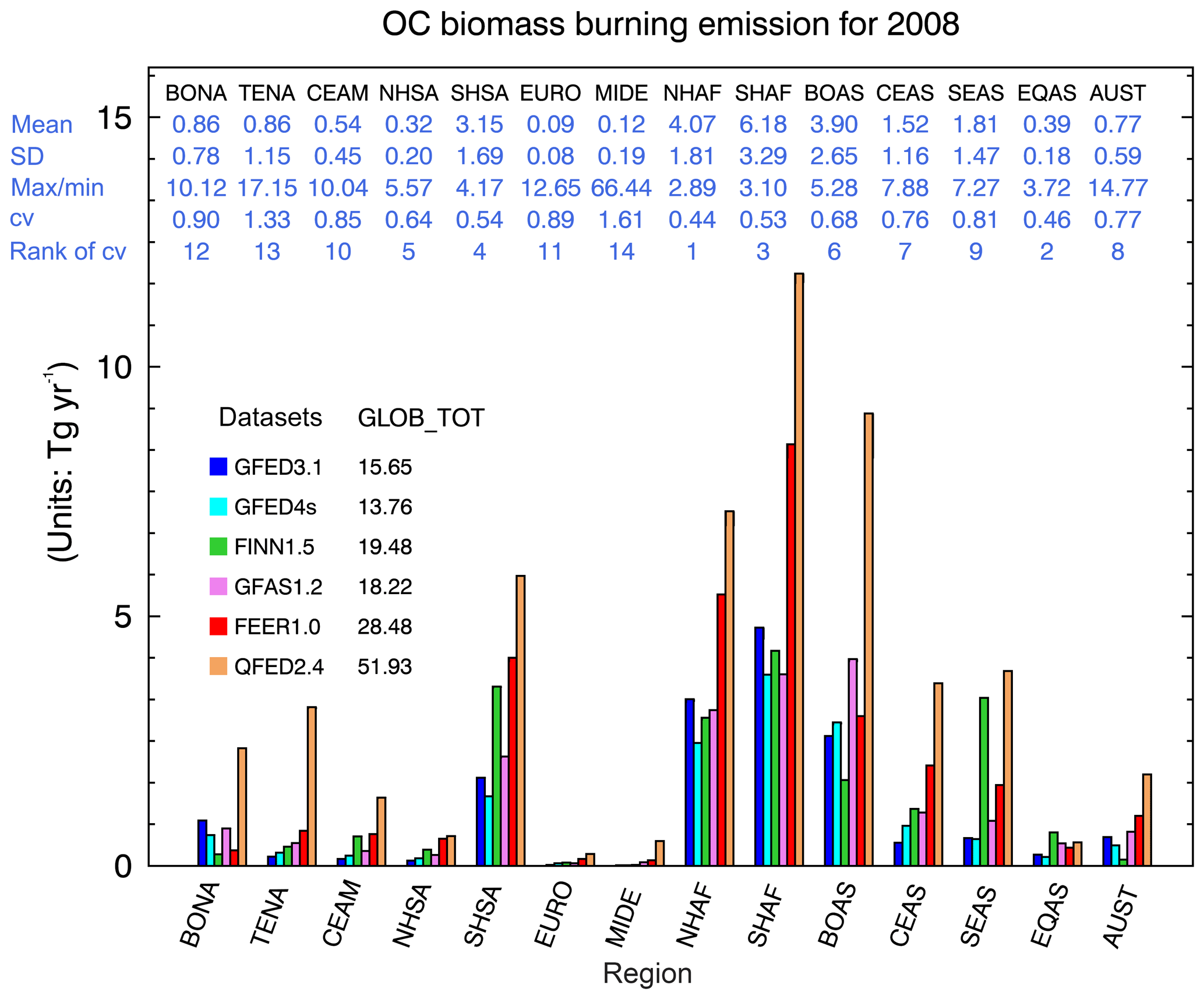
Figure 3The regional annual total organic carbon (OC) biomass burning emissions for 2008 in six biomass burning emission datasets in 14 regions (units: Tg yr−1). The global annual total amount is listed after the name of each dataset (GLOB_TOT). Relevant statistics for the six BB emission datasets in each region are also listed at the top of the panel in blue under the short name of each region, with the mean of the six BB emission datasets in the first row. Three different methods to measure the spread of the six BB emission datasets are shown as well: one absolute method, i.e., the standard deviation (SD) in the second row, and two relative methods, i.e., the ratio of max to min (i.e., maximum ∕ minimum) shown in the third row, as well as the coefficient of variation (cv), defined as the ratio of the SD to the mean, in the fourth row. The rankings of the regions reflecting the spread of the BB emissions datasets according to cv are shown in the fifth row (i.e., a ranking of 1 means that this region shows the least spread among the six BB emissions datasets, while a ranking of 14 indicates that this region has the largest spread among the 14 regions).
Overall, two FRP-based BB emissions, QFED2.4 and FEER1.0, were a factor of 2–4 larger than the other BB datasets. This result is consistent with the findings of Zhang et al. (2014) over sub-Saharan Africa. It is worth noting that the BB emission amount of GFAS1.2 was close to that of GFED3.1, reflecting the fact that GFAS1.2 is tuned to GFED3.1 (described in Sect. 2.1.4). Globally, FINN1.5 yielded more OC emissions than the two GFED datasets and GFAS1.2 (e.g., 40 % larger than GFED4s). Regionally, FINN1.5 was generally comparable to the two GFED datasets in most of the regions, but was higher than them in the tropical regions, such as EQAS, Southeast Asia (SEAS), Central America (CEAM), and Northern Hemisphere South America (NHSA). Interestingly, FINN1.5 was even the largest among all six datasets over the EQAS region, which might be associated with its assumption of continuation of burning into the second day in that region (to be discussed in Sect. 4.1.2). The global OC emissions from GFED4s were lower than those from its GFED3.1 counterpart, although higher in several other regions, such as TENA, CEAM, NHSA, boreal Asia (BOAS), and central Asia (CEAS). Possible explanations for these differences among the six global BB emissions datasets are provided in Sect. 4.1.
3.1.2 Seasonal variation
Biomass burning is generally characterized by distinct seasonal variations in each of the 14 regions and globally, as shown in Fig. 4. Overall, there were four peak fire seasons across the regions: (1) during the boreal spring (March–April–May), fires peak in BOAS mainly because of forest fires (see the contribution of different fire categories in Table 3 of van der Werf et al., 2017); in CEAM, NHSA, and SEAS because of savanna and deforestation fires; and in central Asia (CEAS) mainly due to the agricultural waste burning to prepare the fields for spring crops. (2) During the boreal summer (June–July–August), fires peak in BONA and TENA, mostly due to wildfires that occur under the prevailing dry and hot weather, in EURO probably associated with the burning of agricultural waste. In addition, we found that fire peaked in MIDE in the three FRP-based datasets, i.e., QFED2.4, FEER1.0, and GFAS1.2. This might be associated with the failure to filter out the gas flares from the FRP fire product, especially in QFED2.4 (Darmenov and da Silva 2015). (3) During the austral spring (September–October–November), fires peak in the southern hemispheric regions of SHSA, SHAF, and AUST (Australia and New Zealand), associated with savanna burning (in addition to deforestation fires in SHSA). In SHSA, the two GFED versions peaked in August, 1 month earlier than the rest; (4) during the boreal winter (December and January), fires peak in NHAF, particularly along the sub-Sahel belt (Fig. 2), where savanna fires are associated with agricultural management and pastoral practices across that region (e.g., Ichoku et al., 2016b). Overall, all six BB emission datasets exhibited similar seasonal variations, although they differed in magnitude. In particular, it is noteworthy that in EQAS, the annual OC emissions from GFED4s were lower than those of GFED3.1 by 18 %, but higher by a factor of 2 in the month of August when peatland burning is predominant.
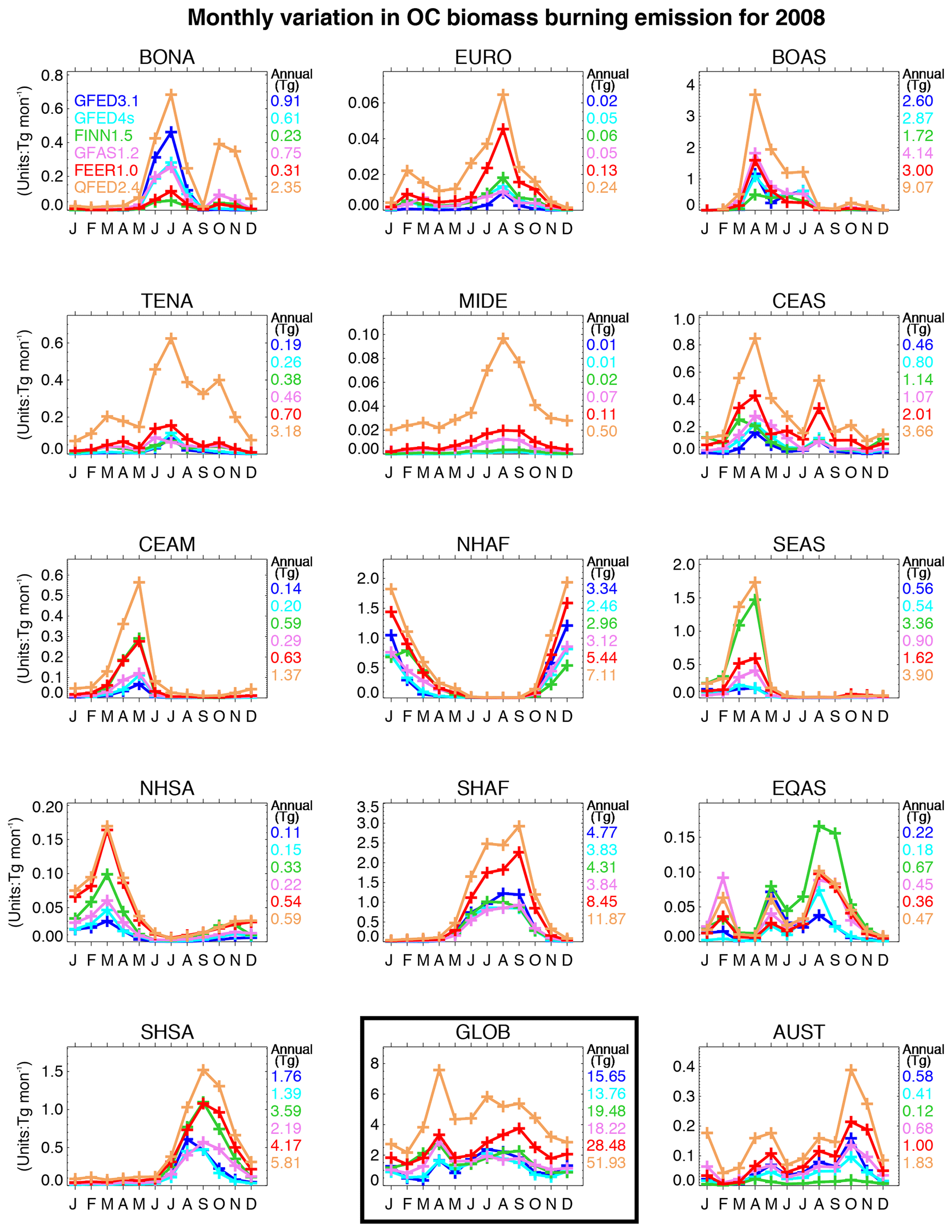
Figure 4Monthly variation in organic carbon (OC) biomass burning emissions for 2008 in six biomass burning emission datasets in 14 regions and the globally (i.e., GLOB, highlighted with a black box). The annual total emission is listed on the right side of each panel.
For reference, biomass burning black carbon (BC) emissions are also shown, but in the Supplement (Figs. S1, S2 for annual total and Fig. S3 for seasonal variation), which exhibited features similar to those of OC. The amounts of biomass burning BC emission were almost proportional to their OC counterparts (about 1∕10 to 1∕15 of OC).
3.2 Comparison of model-simulated AOD with remote sensing data
As in other similar situations where several different datasets are available to be chosen from (e.g., Bian et al., 2007), a question that invariably comes to mind is the following: which BB emission dataset is the most accurate or should be used in a given situation? In fact, it is difficult to give a conclusive answer, as it is often challenging to measure the emission rate of an active fire in real time or to disentangle the contribution of smoke aerosols from the total atmospheric aerosol loading and concentration in observations. Therefore, in this study we have implemented all six global BB emission datasets separately in the GEOS model, and we evaluated their respective simulated aerosol loadings. More specifically, we compared the simulated AOD with the satellite-retrieved AOD data from MISR (primarily to examine the spatial coverage) as well as with ground-based measurements from AERONET sites near biomass burning source regions to examine the seasonal variation. Our analysis was focused on the regional biomass burning peak seasons, when smoke aerosol emissions dominate those from other sources, such as pollution or dust. With such an effort to evaluate the sensitivity of the simulated AOD to the different BB emission datasets, the results from this study may shed some light on the aforementioned question; i.e., which BB dataset is the most accurate or should be used in a given situation? We acknowledge that although the result from a particular model (e.g., GEOS in this case) can potentially introduce additional uncertainty through various complicated and nonlinear procedures employed to calculate the AOD, such as the modeled relative humidity and the related aerosol hydroscopic growth (Bian et al., 2009; Pan et al., 2015), evaluation of the model-simulated AOD has still proven to be a feasible approach to compare various BB emission datasets in reference to the currently available observations (e.g., Petrenko et al., 2012; Zhang et al., 2014).
Aiming to evaluate the sensitivity of the modeled AOD to different BB emissions datasets, we compared the spatial distribution of the GEOS model-simulated AOD with MISR-retrieved AOD in Sect. 3.2.1 and with the AERONET-measured AOD at 14 AERONET sites in Sect. 3.2.2. We also conducted an in-depth study at two AERONET sites, Alta Floresta (in the Southern Hemisphere South America, SHSA) and Mongu (in Southern Hemisphere Africa, SHAF), as discussed in Sect. 3.3.
3.2.1 Global spatial distribution
Comparisons for September and April in 2018 are shown in Figs. 5 and 6, respectively, representing the peak biomass burning months in the Southern Hemisphere and many regions in the Northern Hemisphere, respectively. The MISR AOD is displayed in the top left panel and the model biases (model minus MISR) from the seven individual experiments are shown in the rest of the panels.
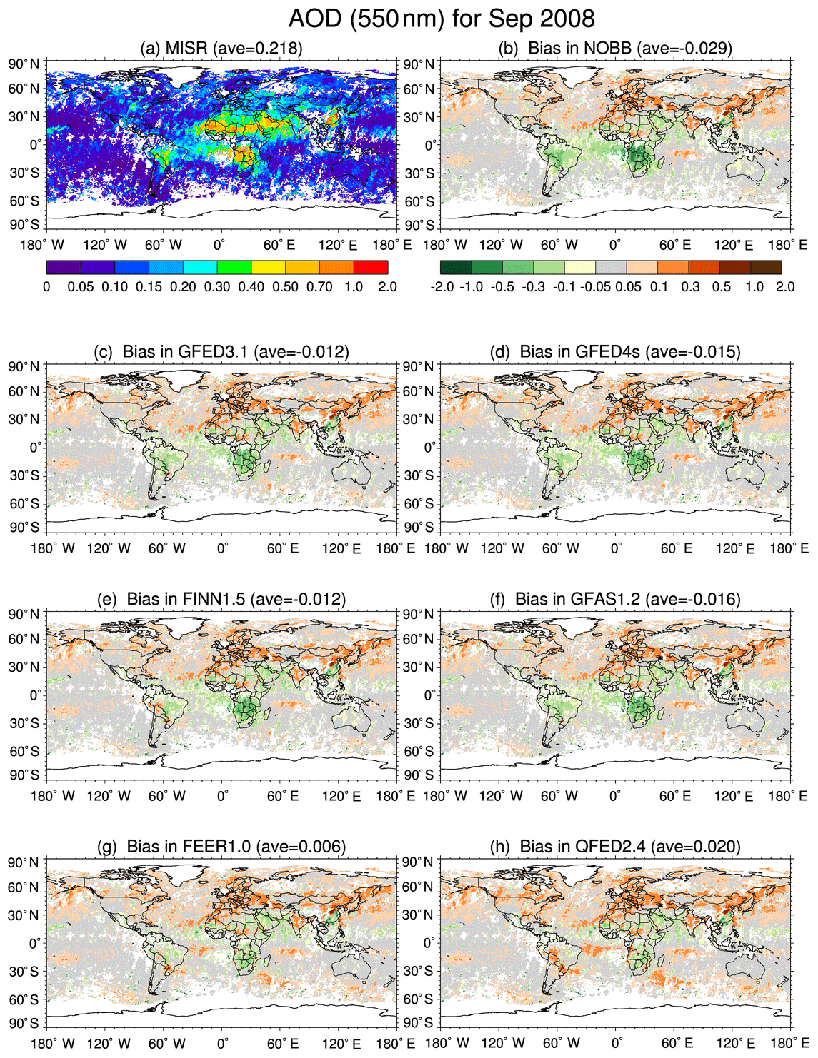
Figure 5(a) The spatial distribution of monthly mean AOD at 558 nm for September 2008 from MISR with white representing missing values. The global average value (ave) is shown in parentheses. Panels (b)–(h) are for GEOS model biases (i.e., model at 550 nm minus MISR at 558 nm) in seven model experiments, i.e., bias in (b) NOBB, (c) GFED3.1, (d) GFED4s, (e) FINN1.5, (f) GFAS1.2, (g) FEER1.0, and (h) QFED2.4.

Figure 6Same as Fig. 5 except for April 2008.
In September 2008, the high AOD observed from MISR (Fig. 5a) in the Southern Hemisphere was mostly attributable to biomass burning. A large fraction of Southern Hemisphere Africa (SHAF) featured high AOD (greater than 0.5). The area-averaged AOD over the entire SHAF was 0.331 (see Table S1 for the area-averaged MISR AOD in each region). The observed AOD peaked in central Africa (nearly 1.0) and gradually decreased westwards. A large negative model bias (−0.283) was found in the NOBB run over the region of SHAF (greenish shading in Fig. 5b; see Table S1 for the area-averaged model biases in each region). The negative bias was reduced most significantly in the QFED2.4 run (see Fig. 5h) to −0.044, followed by the FEER1.0 run (see Fig. 5g) to −0.079, but only to a limited extent in GFED4s and GFAS1.2 (see Fig. 5d and f, respectively), whose biases were still as large as −0.208.
In Southern Hemisphere South America (SHSA), where the area-averaged MISR AOD was 0.188, the maximum AOD was ∼0.7 in central Brazil (Fig. 5a). The negative bias averaged over SHSA was −0.132 in the NOBB run (Fig. 5b). The bias was most significantly reduced in the FEER1.0 run to −0.021 (Fig. 5g), but it appeared overcorrected in the QFED2.4 run to 0.020 (see reddish shading in Fig. 5h). The reduction of negative bias was again the least in the GFED4s run (Fig. 5d) and the GFAS1.2 run (Fig. 5f), whose biases were still as large as −0.081 and −0.080, respectively.
Being mixed with and often surpassed by other aerosol types, however, the contribution of biomass burning aerosols to the total AOD is hardly distinguishable from those of other sources in the peak biomass burning months in certain regions, such as April (Fig. 6) in the regions of Southeast Asia (SEAS), central Asia (CEAS), and boreal Asia (BOAS). Such complicated situations lead to the difficulties in evaluating the BB emission datasets with AOD observations, especially when the background AOD represented by the NOBB run was already overestimated, for example, in the region of CEAS, or when the MISR AOD was missing, for example, in the region of BOAS (where MODIS AOD was missing as well, not shown).
3.2.2 Seasonal variations in AOD at AERONET sites
In order to better quantify the sensitivity of the simulated AOD to the six different BB emission datasets, we further compared the simulated monthly AOD with the ground-based AOD observations from AERONET stations by choosing one representative station in each region (see Fig. 7: the panels representing the AERONET stations in Fig. 7 were arranged in a way that their placements correspond to those of their respective regions in Fig. 4 for easy reference). The exceptions are two regions NHSA and EQAS, where valid AERONET observations could not be found during 2008. Thus, we used the multi-year climatology of AOD at Medellín and Palangkaraya to represent NHSA and EQAS, respectively. We also included the climatology of AERONET AOD in the other 12 AERONET sites for reference. As shown in Fig. 7, the annual cycle of AOD in 2008 at available sites (thin brown bars) was similar to its respective climatology (thick light gray bars) to within 0.05. The MISR AOD was plotted for reference as a green diamond. In this section, the modeled monthly mean AOD was calculated by averaging over the modeled instantaneous AOD in each month, while the monthly AOD of AERONET and MISR was simply calculated by averaging over available observations in each month.
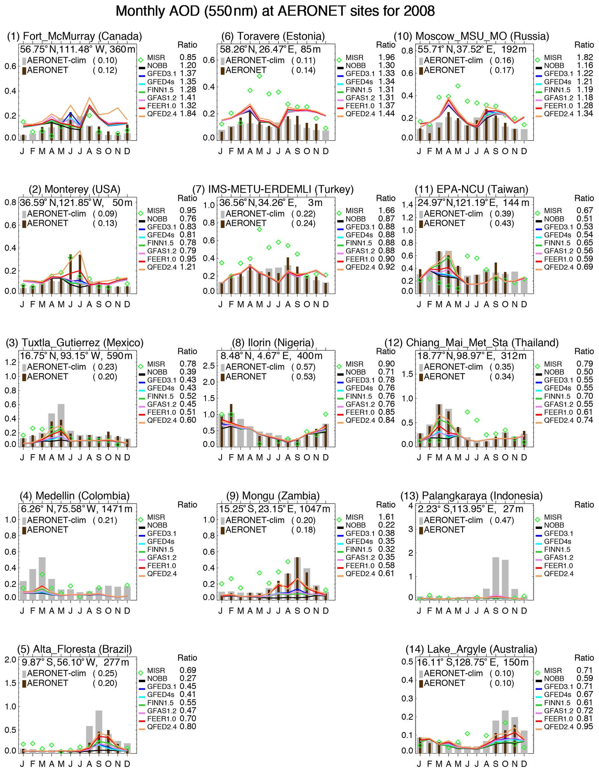
Figure 7Monthly variation in AOD (at 550 nm wavelength) for 2008 over 14 AERONET sites selected from the respective 14 regions (with the country of each site indicated in parentheses). The climatology of AERONET AOD (i.e., AERONET-clim) is represented by thick light gray bars and the monthly mean AERONET AOD for 2008 by thin brown bars, with their corresponding annual mean values shown in parentheses. MISR monthly mean AOD at 558 nm is represented by the green diamonds, and the seven GEOS experiments with different biomass burning emission options are represented by the lines in different colors. The corresponding annual ratios (ratio of model ∕ AERONET) listed on the right-hand side of each panel are estimated by averaging over monthly ratios.
Contributions from non-BB emissions to the total AOD are represented by the NOBB experiment (black line in Fig. 7). Runs with different BB emission datasets showed almost identical AOD during non-biomass-burning seasons at each selected AERONET station in each region, thereby allowing their differences to be noticeable during the biomass burning peak seasons. At Alta Floresta in Brazil (Fig. 7(5)), Mongu in Zambia (Fig. 7(9)), and Chiang Mai Met Sta in Thailand (Fig. 7(12)), where the biomass burning emissions dominated the peak AOD, almost all experiments underestimated AOD during the respective peak biomass burning seasons. However, the fact is that the contribution of non-BB AOD was usually more than that of BB AOD during the burning seasons at most of the selected AERONET sites, except at the above three sites, Therefore, it is difficult to disentangle the effect of biomass burning on the total AOD in most situations, especially when the model has difficulty representing the non-BB AOD, leading, for example, to overestimation at three high-latitude (>55∘ N) AERONET sites (the three panels in the top row of Fig. 7), i.e., Fort McMurray in Canada (Fig. 7(1)), Tõravere in Estonia (Fig. 7(6)), and Moscow_MSU_MO in Russia (Fig. 7(10)). However, it is apparent that the simulated AOD values based on QFED2.4 were overestimated during October and November at Fort McMurray in the USA, indicating that QFED2.4 overestimated BB organic carbon emission during these 2 months. In general, at most of the AERONET sites, the simulated AOD values based on QFED2.4 were the highest and closest to AERONET AOD during the corresponding peak of the biomass burning seasons, followed by FEER1.0 and FINN1.5 and then GFED3.1, GFEDv4, and GFAS1.2.
3.3 Case studies in biomass-burning-dominated regions
In order to investigate the relationship between AOD and biomass burning emission in the context of daily variation, we focused on two AERONET stations, namely Alta Floresta in Brazil and Mongu in Zambia during September, for the in-depth analysis in this section. Biomass burning emissions are known to be dominant at these locations and in this month, as estimated by Chin et al. (2009), who found that 50 %–90 % of the AOD was attributable to biomass burning emissions according to GOCART model simulations. Based on other previous studies as well, e.g., two studies with multiple BB datasets applied to one model, Pereira et al. (2016) in Southern Hemisphere South America and Reddington et al. (2016) in tropical regions including Southern Hemisphere South America and Africa or the AeroCom Multi-model study (Mariya Petrenko, personal communication, 2019) with one biomass burning emission dataset (i.e., GFED3.1) mentioned earlier in the introduction, there appears to be a general consensus that the simulated AOD is consistently underestimated over Southern Hemisphere South America and Africa in many models. Therefore, in this study, we further examined these two sites: Alta Floresta in Brazil and Mongu in Zambia. We calculated the 3-hourly AOD by sorting the instantaneous AOD from both AERONET and model outputs for each day into eight time steps, namely 0, 3, 6, 9, 12, 15, 18, and 21Z. The modeled monthly mean AOD was calculated by averaging over the modeled 3-hourly AOD, which coincided with 3-hourly AERONET AOD in that month. The detailed analyses are discussed below.
3.3.1 Alta Floresta in Brazil (Southern Hemisphere South America, SHSA)
The monthly mean AOD observed from AERONET at Alta Floresta is 0.47 during September 2008 (Fig. 8a). It shows that the simulated AOD from all six experiments captured the high aerosol episode observed in the AERONET dataset during 13 September (AERONET AOD is about 1.0–1.2). The simulation with QFED2.4 BB emission produced the closest agreement with the AERONET observed AOD with an average ratio of 1.00. In contrast, the simulated AOD with FEER1.0 (ratio =0.73), FINN1.5 (ratio =0.55), GFAS1.2 (ratio =0.42), GFED3.1 (ratio =0.40), and GFED4s (ratio =0.36) tended to be underestimated most of the time. All experiments showed relatively low skill at capturing the temporal variability of the observed AOD at Alta Floresta (corr =0.24–0.60). The Ångström exponent (AE: an indicator of particle size) from AERONET is 1.66 (not shown), indicating that small particles, most likely those from smoke, dominated the total aerosol loading at Alta Floresta (Eck et al., 2001). All experiments matched the observed AE (not shown).

Figure 8Characteristics of the observed and the simulated aerosols at Alta Floresta during September 2008: (a) the 3-hourly time series of AOD at 550 nm. The AERONET AOD is represented by vertical gray bars, and the outputs from the six model experiments are represented by the color curves. The relevant statistics are listed: ave is the monthly average, ratio is the fraction of the simulated to the observed AOD at all observed hours, corr is correlation coefficient between the observed and the simulated AOD, and RMSE is root-mean-square error. (b) The 3-hourly time series of OC column mass density over the grid box where Alta Floresta is located (units: kg m−2 or mg m−2). (c) Same as panel (b) but for biomass burning OC emission rate (units: kg m−2 s−1 or µg m−2 s−1). (d) MODIS Terra true-color image around Alta Floresta on 13 September 2008, overlaid with the active fire detections as red dots (image credit: https://aeronet.gsfc.nasa.gov/cgi-bin/bamgomas_interactive, last access: 29 December 2018, and https://worldview.earthdata.nasa.gov, last access: 29 December 2018).
The OC column mass loading (Fig. 8b) in each run resembled its corresponding AOD (Fig. 8a), implying that the day-to-day variation in OC column mass loading in this dry season dominates the simulated AOD in the model, rather than other factors such as relative humidity (RH). The OC column mass loading is determined by the regional scale of emission, transport, and removal processes of aerosols; the latter two processes being the same across the six experiments, given that the same model configurations were used. Therefore, the differences of OC column mass loading and thus AOD across the six experiments are attributed to the different choices of biomass burning emission datasets. Figure 8c shows the local biomass burning OC emissions (i.e., at the grid box where this site is located) in the different biomass burning emission datasets. We found that there was a large contrast in the local biomass burning OC emission between 25 September (as high as 1–2 µg m−2 s−1) and the other days (close to zero) across all six experiments although to different degrees. Similar emission patterns are found when averaged over nine or 25 surrounding grid boxes (not shown). Such a sharp contrast was completely absent in the simulated OC column mass density (Fig. 8b) and AOD (Fig. 8a).
All of the foregoing evidence collectively suggests that the temporal variations in AOD (and aerosol mass loading) in Alta Floresta during the burning season do not directly respond to the local BB emission at the daily and sub-daily timescales but rather to the regional emission. The regional emission is further adjusted by the multiple processes determining the residence time of aerosols in air (typically a few days), such as the regional-scale transport and removal of aerosols. The MODIS Terra true-color image overlaid with active fire detections (red dots) on 13 September 2008 (Fig. 8d) confirms that there were no active fires (represented by red dots) detected at Alta Floresta (blue circle), and thus the dense smoke over the site during this peak aerosol episode must have been transported from the upwind areas rather than from localized BB emission sources. Therefore, accurate estimation of both the magnitude and spatial pattern of regional emissions is quite important.
3.3.2 Mongu in Zambia (Southern Hemisphere Africa, SHAF)
The case of Mongu is different from that of Alta Floresta. Figure 9d reveals that there were numerous active fire detections (represented by the red dots in this MODIS Aqua true-color image) at and close to Mongu (blue circle) on 12 September 2008, one of peak aerosol episodes as Fig. 9a shows. The simulated AOD from all six experiments captured two peak aerosol episodes observed from the AERONET dataset during 11–12 and 2–3 September (AOD about 1.0), albeit underestimated (Fig. 9a). All experiments also underestimated the sustained aerosol episode after 20 September. However, all model experiments almost reproduced the AERONET AE value of 1.80 throughout September at this site (not shown), confirming that the dominance of the fine-mode aerosol particles in smoke aerosols is captured by the model irrespective of the BB emission dataset used.
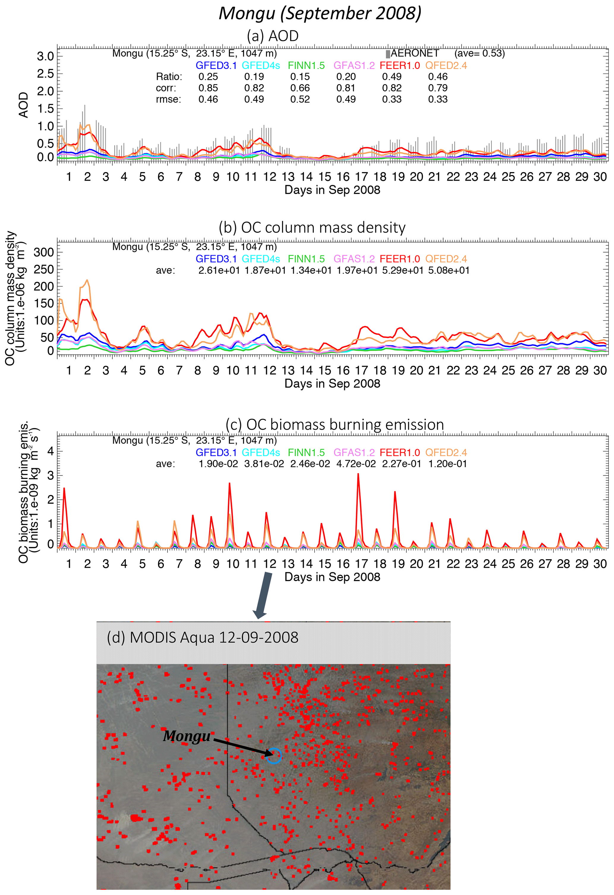
Figure 9Characteristics of the observed and the simulated aerosols at Mongu during September 2008: (a) the 3-hourly time series of AOD at 550 nm. The AERONET AOD is represented by vertical gray bars, and the outputs from the six model experiments are represented by the color curves. The relevant statistics are listed: ave is the monthly average, ratio is the fraction of the simulated to the observed AOD at all observed hours, corr is correlation coefficient between the observed and the simulated AOD, and RMSE is root-mean-square error. (b) The 3-hourly time series of OC column mass density over the grid box where Mongu is located (units: kg m−2 or mg m−2). (c) Same as panel (b) but for biomass burning OC emission rate (units: kg m−2 s−1 or µg m−2 s−1). (d) MODIS Aqua true-color image around Mongu on 12 September 2008, overlaid with the active fire detections as red dots (image credit: https://aeronet.gsfc.nasa.gov/cgi-bin/bamgomas_interactive and https://worldview.earthdata.nasa.gov).
The biomass burning OC emissions averaged over the grid box of Mongu exhibited distinct daily variations in each BB dataset (Fig. 9c). Similar emission patterns are found when averaged over nine or 25 surrounding grid boxes (not shown). At this site, the day-to-day variations in AOD still cannot be totally explained by the corresponding local emission at Mongu. For example, emission from FEER1.0 on 17 September is 6 times higher than that on 2 September (Fig. 9c), but the simulated AOD on 17 September is 2 times lower than that on 2 September (Fig. 9a). However, the magnitude of AOD at Mongu in each experiment corresponded to the magnitude of BB emission at the regional scale, since it is apparent that the overall higher regional BB emissions still resulted in higher column mass loading and thus AOD. For instance, FEER1.0 and QFED2.4, which have the largest monthly total biomass burning OC emission over the region of SHAF among the six BB emission datasets during September (2.27 and 2.92 Tg per month, respectively, as shown in Fig. 4), corresponded to the highest AOD (ratio =49 % and 46 %, respectively, as shown in Fig. 9a), while FINN1.5 and GFED4s, which represent the lowest monthly mean biomass burning OC emission over the region of SHAF (0.87 and 0.85 Tg per month, respectively, as shown in Fig.4), corresponded to very low AOD (15 % and 19 % of the observed AOD, respectively).
Although the temporal variation in the ambient RH may partially contribute to the day-to-day changes of the emission–AOD relationship, the close resemblance between the model-simulated AOD and column OC mass loading (Fig. 9b) excludes such possibility. This evidence therefore suggests that the temporal variations in AOD (and aerosol mass loading) in Mongu, where daily local BB emissions were present instead, do not directly respond to the local BB emission at the daily and sub-daily timescales during the burning season either as is the case in Alta Floresta. It further confirms the importance of accurate estimation of both the magnitude and spatial pattern of regional emissions as mentioned in the case of Alta Floresta. Therefore, over Southern Hemisphere Africa and Southern Hemisphere South America, an enhancement of regional BB aerosol emission amounts in all the BB emission datasets except for QFED2.4 in the latter region is suggested by this study in order to reproduce the observed AOD level although to different degrees.
The simulated AOD is biased low in biomass-burning-dominated regions and seasons across almost all six BB emission datasets as demonstrated in this study. More explanations on differences among the six BB emissions datasets are discussed in Sect. 4.1. Basically, the uncertainty of the simulated AOD could be attributable to two main sources: (1) BB emissions-related biases and (2) model-related biases. They are discussed in Sect. 4.2 and 4.3, respectively.
4.1 The possible explanations of differences among the six BB emission datasets
4.1.1 Higher BB emissions estimated from QFED2.4 and FEER1.0
This study has shown that the QFED2.4 and FEER1.0 BB emission datasets are consistently higher than the others, with QFED2.4 being the highest overall. Some of the possible reasons responsible for this difference include the following.
-
Constraining with MODIS AOD. The emission coefficients (Ce) used to derive biomass burning aerosol emissions in both QFED2.4 and FEER1.0 are constrained by the MODIS AOD, although in different ways (detailed in Sect. 2.1.6 and 2.1.5, respectively). This is not the case for the other BB emission datasets. Although GFAS1.2 uses the same FRP products as FEER1.0 in deriving dry mass combustion rate, its emission is tuned to that of GFED3.1. QFED2.4 applied four biome-dependent scaling factors to the initial constant value C0 when deriving its Ce, by minimizing the discrepancy between the AOD simulated by the GEOS model and that from MODIS in corresponding biomes. The resulting QFED2.4 scaling factors are 1.8 for savanna and grassland fires, 2.5 for tropical forests, and 4.5 for extratropical forests (Darmenov and da Silva, 2015). This partially explains its very high OC biomass burning emission over the extratropical regions of TENA, BONA, and BOAS relative to the other emission datasets (Figs. 2–4). However, the high BB emission estimated by QFED2.4 is questionable during October and November of 2008 in the region of BONA (Fig. 4) according to the evaluation of its resulting AOD relative to the AERONET AOD at the Fort McMurray site (Fig. 7(1)). As for FEER1.0, the process of deriving Ce involved calculating the near-source smoke–aerosol column mass with the MODIS AOD (total minus the background) for individual plumes, thereby limiting influence from other emission sources (Ichoku and Ellison, 2014).
-
Fuel consumption. In general, the FRP-based estimation approaches, such as GFAS1.2, QFED2.4, and FEER1.0, may enable more direct estimates of fuel consumption from energy released from fires, without being affected by the uncertainties associated with the estimates of fuel loads and combustion completeness (e.g., Kaufman et al., 1998; Wooster et al., 2003, 2005; Ichoku and Kaufman, 2005; Ichoku et al., 2008; Jordan et al., 2008). However, FRP from non-BB sources, such as the gas flare, could be mistakenly identified as BB sources. One example is over bare land on the eastern border of Algeria in MIDE (refer to the land type on the website http://maps.elie.ucl.ac.be/CCI/viewer/index.php, last access: 17 January 2020), where QFED2.4 shows high OC emission contrary to expectation (see Fig. 2f). Thus, additional screening of the FRP fire product is required.
4.1.2 Features of FINN1.5
Globally, the FINN1.5 dataset is lower than QFED2.4 and FEER1.0 but larger than GFAS1.2, GFED3.1, and GFED4s (Fig. 3). Although FINN1.5 can capture the location of the large wildfires using the active fire products, the estimation of burned area is rather simple without the complicated spatial and temporal variability in the amount of burned area per active fire detection or variability in fuel consumption within biomes. For example, it estimates 1 km2 of burned area per fire pixel for all biomass types except for savanna and grassland where 0.75 km2 per fire pixel is estimated instead. That might partially explain why FINN1.5 is extremely low in AUST, as suggested by Wiedinmyer et al. (2011). Additionally, the FINN1.5 dataset is the least over boreal regions, such as in the regions of BOAS and BONA, where FINN1.5 is only one-third and three-fifths of GFED4s, respectively. Large forest fires dominate in BOAS and BONA, such that the direct mapping of burned area as calculated in GFED4s and GFED3.1 produces more biomass burning emissions (van der Werf et al., 2017). On the other hand, the BB emission in the FINN1.5 dataset is relatively large near the Equator. For instance, it is the largest among the six datasets over the region EQAS and the second largest over the regions of CEAM and SEAS (see Fig. 3). This might be attributed to the smoothing of the fire detections in these tropical regions to compensate for the limited daily coverage by the MODIS instruments due to gaps between adjacent swaths and higher chances of cloud coverage in tropical regions (Wiedinmyer et al., 2011). Thus, in FINN1.5, each fire detected in the equatorial region is only counted for a 2 d period by assuming that fire continues into the next day but at half of its original size.
4.1.3 Difference between GFED4s and GFED3.1
Globally and in some regions, biomass burning OC emission in GFED4s is lower than that in GFED3.1 (see Figs. 2–4), although the former has 11 % higher global carbon emissions and includes small fires (van der Werf et al., 2017). There are a few possible reasons, of which two major ones are as follows: (1) for aerosols, the implementation of lower EF for certain biomes in GFED4s than in GFED3.1 reduces the aerosol biomass burning emissions. As for the savanna and grassland, for instance, the GFED4s dataset mainly applies the EF value recommended by Akagi et al. (2011), which is 2.62 g OC kg−1 dry matter burned, 18 % lower than the EF from Andreae and Merlet (2001) used in GFED3.1, which is 3.21 g OC kg−1 dry matter burned (see Table 2). The new estimation of EF is 3.0±1.5 g OC kg−1 dry matter burned as suggested by Andreae (2019). With it, the OC emissions in savanna and grassland can be slightly enhanced but would still be lower than those in GFED3.1. (2) The improvement in including small fires in GFED4s over GFED3.1 is probably offset by the occasional optimization of fuel consumption using field observations for overall carbon emissions. For instance, the turnover rates of herbaceous leaf vegetation (e.g., savanna) are increased in GFED4s, leading to the lower fuel loading and thus lower consumption for this land-cover type in GFED4s (van Leeuwen et al., 2014; van der Werf et al., 2017). Therefore, the biomass burning OC emissions are lower in GFED4s over SHAF, NHAF, and AUST (Figs. 3 and 4), where ∼88 % of the BB carbon emission is from savanna and grassland (van der Werf et al., 2017).
Table 2Comparison of emission factor (units: g species kg−1 dry matter burned) used by GFED3.11 and GFED4s2 (listed in the upper and lower parts of the cell, respectively, and bold if GFED4s is larger).

1 Mainly from Andreae and Merlet (2001) with annual updates. 2 Mainly from Akagi et al. (2011), supplemented by Andreae and Merlet (2001) and other sources. 3 GFED4s (van der Werf et al., 2017) further divides extratropical forest in GFED3 (van der Werf et al., 2010) into temperate forest and boreal forest. 4 Based on Christian et al. (2003) for CO2 and CO.
On the other hand, there are regions in the Northern Hemisphere where GFED4s is higher than GFED3.1. For example, over CEAS and EURO, small fires associated with burning of agricultural residues contribute to 43.6 % and 58.6 % of the carbon emissions, respectively (van der Werf et al., 2017). In spite of the 30 % reduction of the EF in these two regions, the effect of including small fires in GFED4s is greater, resulting in the biomass burning OC emission from GFED4s being twice as high as that from GFED3.1. Another example is in BOAS where the biomass burning OC emissions are 10 % higher in GFED4s than in GFED3.1. This is likely attributable to the higher EF used in GFED4s for boreal forest fires than that in GFED3.1 (9.60 vs. 9.14 g OC kg−1 dry matter; see Table 2), where 86.5 % of the carbon emission is from the Siberian forest (van der Werf et al., 2017).
It is interesting that the yearly total biomass burning OC emission from GFED4s is 20 % lower than that from GFED3.1 in EQAS (Fig. 4), even though the small fires are included and the EFs of peatland and tropical forest are higher in the former (Table 2). By examining the monthly variations over EQAS (Fig. 4), however, we found that GFED4s is actually higher than GFED3.1 in August by a factor of 2 when peatland burning is predominant but is equal to or lower than GFED3.1 in other months, particularly in May, leading to the overall lower annual total value in GFED4s.
4.2 Sources of the uncertainty associated with biomass burning emissions
Uncertainty in any of the six BB emissions datasets considered in this study could have been introduced from a variety of measurement and/or analysis procedures, including detection of fire or area burned, retrieval of FRP, emission factors (see Table 1), biome types, burning stages, and fuel consumption estimates, some of which are explained in detail below.
-
Fire detection. Most of the current global estimations of biomass burning emissions are heavily dependent on polar-orbiting satellite measurements from MODIS Terra and Aqua (e.g., MCD14DL, MOD14A1, MYD14A1, and MCD14ML as listed in Table 1). The temporal and spatial resolutions of these measurements impose limitations on their ability to detect and characterize the relevant attributes of fires, such as the locations and timing of active fires and the extent of the burned areas. Each of the two MODIS sensors, from which all of the major BB datasets derive their inputs, can only possibly observe a given fire location twice in 24 h, which leaves excessive sampling gaps in the diurnal cycle of fire activity (Saide et al., 2015). Even for these few times that MODIS makes observations at its nominal spatial resolution of 1 km at nadir, it has the potential to miss a significant number of smaller fires (e.g., Hawbaker et al., 2008; Burling et al., 2011; Yokelson et al., 2011), as well as to miss fires obstructed by clouds, and those located in the gaps between MODIS swaths in the tropics (Hyer and Reid, 2009; Wang et al., 2018). In addition, MODIS fire detection sensitivity is reduced at MODIS off-nadir views, with increasing view zenith angles, especially toward the edge of scan, where its ground pixel size is almost a factor of 10 larger that at nadir (Peterson and Wang, 2013; Roberts et al., 2009; Wang et al., 2018), resulting in dramatic decreases in the total number of detected fire pixels and total FRP (Ichoku et al., 2016b; Wang et al., 2018). Moreover, all operational remote sensing fire products have difficulty accounting for understory fires or fires with low thermal signal or peatland fires such as those in Indonesia, where smoldering can last for months (Tansey et al., 2008). These issues can propagate into the uncertainties of the emissions datasets that are dependent on active fire detection products, especially those based on FRP, e.g., GFAS1.2 (Kaiser et al., 2012), FEER1.0 (Ichoku and Ellison, 2014), and QFED2.4 (Darmenov and da Silva, 2015). This issue also affects FINN1.5 (Wiedinmyer et al., 2011), which derives the burned area by assuming each active fire pixel to correspond to a burned area of 1 km2 for most biome types (see details in Sect. 2.1.3), and GFED4s, which uses burned area product for large fires but derives burned areas for small fires using the MODIS active fire product.
On the other hand, although the sparse diurnal sampling frequency may not necessarily be an issue for the MODIS burned area product, upon which some of the emission datasets are based (e.g., GFED3.1), burned area product may not account for small fires due to its low spatial resolution of 500 m, which may limit the identification of small burned scars such as those generated by small fires from croplands. In addition, the estimation of biomass burning emission based on the burned area product, e.g., GFED, is subject to the uncertainty associated with the estimation of fuel load and combustion completeness as mentioned earlier.
-
Emission factor (EF). The EF, used for deriving individual particulate or gaseous species of smoke emissions from burned dry matter in all major BB emission datasets, heavily depends on the two papers by Andreae and Merlet (2001) and Akagi et al. (2011). The authors of these two studies made significant contributions by compiling the values of EFs from hundreds of papers. However, the EFs can have significant uncertainties (Andreae, 2019), because each EF results from a particular experiment or field campaign. Some EFs are derived from lab-based studies whereby samples of fuels are burned in combustion chambers (e.g., Christian et al., 2003; Freeborn et al., 2008), where the combustion characteristics can be very different from those of large-scale open biomass burning and wildfires, and some EFs are derived from field campaigns, where the measurement locations are often not close enough to the biomass burning source due to personnel safety and other logistic factors (Aurell et al., 2019). As discussed earlier in Sect. 4.1.3, the discrepancy between GFED4s and GFED3.1 can be partially explained by the fact that different emission factors were used to derive these two products (also see Table 2). This situation will not change much even if the EF value from the latest estimation by Andreae (2019) were used.
-
Biome types. The uncertainty of estimating BB emission could be partially attributed to different definitions of major biome types, because the scaling factor of emission coefficient for the FRP-based BB datasets (i.e., GFAS and QFED) or the emission factor used by all BB datasets will be assigned according to the biome type where the fire event occurs. The six BB emission datasets examined in this study have different definitions of major biome types, for example, there are six major biome types applied in GFED4.1s (Table 1 in van der Werf et al., 2017), but eight in GFAS1.2 (Table 2 in Kaiser et al., 2012), and only four in QFED2.4 (Table 2 in Darmenov and da Silva, 2015). In particular, peat combustion is an important emission source in some regions, such as equatorial Asia (e.g., Kiely et al., 2019). However, not all the emission datasets include peat biome or consider its unique characteristics. Among the emission datasets based on burned areas, GFED3.1 and GFED4s consider peat, but FINN1.5 does not. In QFED2.4 and FEER1.0, the peat biome is not explicitly identified. Thus, such differences in the approaches to the processing of contributions from specific biomes may contribute to the differences between emission datasets in some regions.
-
Burning stages. Most current BB emission datasets do not distinguish the different burning stages, such as the flaming and smoldering stages that have distinctive emission characteristics. Typically, flaming dominates the earlier stage of a fire while smoldering dominates the later part. In the case of boreal forest fires, for example, about 40 % of the combustion originates from the flaming phase while 60 % comes from the smoldering phase (Reid et al., 2005). In addition, smoldering combustion produces more OC and CO than flaming combustion, whereas flaming combustion produces more BC and carbon dioxide (CO2) than smoldering (e.g., Freeborn et al., 2008).
4.3 Sources of the uncertainty associated with aerosol modeling
The model-related biases in the GEOS model, which other models most probably also suffer from, include, for example, inaccurate representations of horizontal and vertical transport of aerosol by wind, fire emission plume height, and estimation of aerosol removal in models. Furthermore, the production of secondary organic aerosol (SOA) in biomass burning plumes, which has been observed in lab studies and ambient plumes (e.g., Bian et al., 2017; Ahern et al., 2019), is missing in these GEOS simulations. Given the sparsity of the measurements of surface and vertical concentrations at the global scale, we implemented an approach to evaluate model simulation uncertainty globally due to biomass burning aerosol emissions by evaluating the resulting AOD against that from satellite data and AERONET measurements, following the studies by Petrenko et al. (2012) and Zhang et al. (2014). We acknowledge the uncertainties in calculating AOD, such as uncertainties associated with assumptions of aerosol size distribution, optical properties, aerosol water uptake, and vertical distribution of aerosol (e.g., Reddington et al., 2019). In addition, Ge et al. (2017) showed that the choice of different meteorological fields can also lead to uncertainty in simulating the modeled aerosol loading. For instance, meteorological fields from ECMWF and the National Centers for Environmental Prediction (NCEP) can yield a factor of 2 difference in the resulting surface PM2.5 concentration during the fire season of September in the Maritime Continent. Furthermore, the ratio of OA to OC is 1.4 in our study, as first determined by White and Roberts (1977). However, this OA∕OC ratio of 1.4 is at the low end of the generally suggested range of 1.2–2.5 (Turpin and Lim, 2001; Zhang et al., 2005; Bae et al., 2006; El-Zanan et al., 2005; Aiken et al., 2008; Chan et al., 2010). Observations suggest that OA∕OC values of 1.6±0.2 should be used for urban aerosols and 2.1±0.2 for nonurban aerosols (Turpin and Lim, 2001). Enhancing this ratio can obviously increase the resulting AOD, but a more accurate measurement of this ratio during biomass burning is needed.
In this study, we compared six global biomass burning aerosol emission datasets in 2008, i.e., GFED3.1, GFED4s, FINN1.5, GFAS1.2, FEER1.0, and QFED2.4. We also examined the sensitivity of the modeled AOD to the different BB emission datasets in the NASA GEOS model globally and in 14 regions. The main results are summarized as follows.
The biomass burning OC emissions derived from GFED3.1, GFED4s, FINN1.5, GFAS1.2, FEER1.0, and QFED2.4 can differ by up to a factor of 3.8 on an annual average, with values of 15.65, 13.76, 19.48, 18.22, 28.48, and 51.93 Tg C in 2008, respectively. The biomass burning BC emissions can differ by up to a factor of 3.4 on an annual average, with values of 1.76, 1.65, 1.83, 1.99, 3.66, and 5.54 Tg C in 2008, respectively. In general, higher biomass burning OC and BC emissions are estimated from QFED2.4 globally and regionally, followed by FEER1.0.
The best agreement among the six emission datasets occurred in Northern Hemisphere Africa (NHAF), equatorial Asia (EQAS), Southern Hemisphere Africa (SHAF), and Southern Hemisphere South America (SHSA), where the biomass burning emissions are predominant in determining aerosol loading, with the top coefficient of variation rankings (1–4) and relatively low ratio (a factor of 3–4). The least agreement occurred in the Middle East (MIDE), temperate North America (TENA), boreal North America (BONA), and Europe (EURO), with the bottom coefficient of variation rankings (14–11) and large ratios (a factor of 66–10). It seems that the diversity among the six BB emission datasets is largely driven by QFED2.4, which estimates the largest emission amount for almost all regions (except for equatorial Asia).
In Southern Hemisphere Africa (SHAF) and Southern Hemisphere South America (SHSA) during September 2008, where and when biomass burning aerosols are dominant over other aerosol types, the amounts of biomass burning OC emissions from QFED2.4 and FEER1.0 are at least double those from the remaining four BB emission datasets. The AOD values simulated by the NASA GEOS based on these two BB emission datasets are the closest to those from MISR and AERONET, but still biased low. In particular, at Alta Floresta in SHSA, they can account for 36 %–100 % of the observed AOD, and at Mongu in SHAF the AOD values simulated with the six biomass burning emission datasets only account for 15 %–49 % of the observed AOD. Overall, during the biomass burning peak seasons at most of the representative AERONET sites selected in each region, the AOD simulated with QFED2.4 is the highest and closest to AERONET and MISR observations, followed by that of FEER1.0. Considering that regional-scale transport and removal processes as well as wind fields are the same across the six BB emission experiments since they were run under the same model configurations except for BB emission, it is evident that enhancement of BB emission amounts in all six BB emission datasets will be needed (although to different degrees) for the model AOD simulations to match observations, particularly in SHAF (Mongu) and SHSA (Alta Floresta), except for QFED2.4 in SHSA. Although the result of this study is partially model-dependent, it sheds some light on our understanding of the uncertainty of the simulated AOD associated with the choice of biomass burning aerosol emission datasets.
Based on the results of the current study, it is appropriate to make some recommendations for future studies on improving BB emission estimation. Our understanding of the complexity, variability, and interrelationships between different fire characteristics (behavior, energetics, emissions) still needs to be improved (Hyer et al., 2011). More accurate estimation of emission factors (EFs) for different ecosystem types and burning stages would greatly improve the emission overall, as demonstrated by the discrepancy between GFED3.1 and GFED4s (see Sect. 4.1.3). The global BB emission datasets driven by fire remote sensing and retrievals of FRP and burned-area products, which have hitherto depended heavily on MODIS, can be augmented with products from higher-resolution sensors such as the Visible Infrared Imaging Radiometer Suite (VIIRS) and the global suite of geostationary meteorological satellites such as Meteosat (covering Europe, Africa, and the Indian Ocean), Geostationary Operational Environmental Satellite (GOES, covering North, Central, and South America), and Himawari (covering east Asia, Southeast Asia, and Australia). Also, measurements from the recent field campaigns such as WE-CAN (https://www.eol.ucar.edu/field_projects/we-can, last access: 17 January 2020) and FIREX-AQ (https://www.esrl.noaa.gov/csd/projects/firex-aq/science/motivation.html, last access: 17 January 2020) are expected to contribute toward advancing our knowledge of biomass burning emissions in North America. The evaluation in this study has been solely based on remotely sensed AOD data, including retrievals from both satellite (MISR) and ground-based (AERONET) sensors. Continuous mass concentration measurements are needed to validate the fire-generated aerosol loading in specific contexts, such as in analyzing collocated surface and vertical aerosol concentrations and composition, at least in the major BB regions.
The GFED3.1 biomass burning dataset can be accessed through the link https://daac.ornl.gov/VEGETATION/guides/global_fire_emissions_v3.1.html (van der Werf et al., 2010). The link to the GFED4s dataset is http://www.globalfiredata.org (van der Werf et al., 2017). The FINN1.5 emissions dataset is archived at http://bai.acom.ucar.edu/Data/fire/ (Wiedinmyer et al., 2011). The GFAS1.2 emissions dataset is available at https://apps.ecmwf.int/datasets/data/cams-gfas/ (Kaiser et al., 2012). The FEER1.0 dataset is available at http://feer.gsfc.nasa.gov/data/emissions/ (Ichoku and Ellison, 2014). The QFED2.4 can be downloaded from the website https://portal.nccs.nasa.gov/datashare/iesa/aerosol/emissions/QFED/v2.4r6/ (Darmenov and da Silva, 2015). MISR level 3 AOD data can be downloaded from the website https://eosweb.larc.nasa.gov/project/misr/mil3mae_table (Kalashnikova and Kahn, 2006). AERONET Version 3 Level 2.0 data can be downloaded from the websites https://aeronet.gsfc.nasa.gov/new_web/download_all_v3_aod.html (Holben et al., 1998; Giles et al., 2019). The GEOS model results can be obtained by contacting the corresponding author.
The supplement related to this article is available online at: https://doi.org/10.5194/acp-20-969-2020-supplement.
CI, MC, and XP conceived this project. XP conducted the data analysis and the model experiments. XP and CI wrote the majority of this paper, and all other authors participated in the writing process and interpretation of the results. HB, AD, PC, and AdS helped with model setup. CI, AD, and LE provided the biomass burning emission datasets and interpretation of these datasets. TK, JW, and GC provided the help to apply the biomass burning emission datasets in the model. CI, MC, and TO provided funding support.
The authors declare that they have no conflict of interest.
The contents of this article are solely the responsibility of the authors and do not represent the official views of any agency or institution.
We thank the AERONET networks for making their data available. Site PIs and data managers of those networks are gratefully acknowledged. We acknowledge the use of imagery from the NASA WorldView application (https://worldview.earthdata.nasa.gov), part of the NASA Earth Observing System Data and Information System (EOSDIS). Computing resources supporting this work were provided by the NASA High-End Computing (HEC) Program through the NASA Center for Climate Simulation (NCCS) at the Goddard Space Flight Center. We also thank the providers of biomass burning emission datasets of GFED, FINN, and GFAS. We appreciate the constructive comments from the two reviewers, which helped us to improve the quality of this paper. Xiaohua Pan also acknowledges the valuable suggestions from Dongchul Kim.
This research has been supported mainly by various NASA Earth science programs, including the NASA Atmospheric Composition Modeling, Analysis, and Prediction Program (ACMAP), the Modeling, Analysis, and Prediction program (MAP), the Interdisciplinary Studies Program (IDS), the Carbon Cycle Science program (grant no. NNX14AM76G), and the Educational Partnership Program of the National Oceanic and Atmospheric Administration (NOAA), U.S. Department of Commerce, under agreement no. NA16SEC4810006.
This paper was edited by Dominick Spracklen and reviewed by Mark Parrington and one anonymous referee.
Ahern, A. T., Robinson, E. S., Tkacik, D. S., Saleh, R., Hatch, L. E., Barsanti, K. C., Stockwell, C. E., Yokelson, R. J., Presto, A. A., Robinson, A. L., Sullivan, R. C., and Donahue, N. M.: Production of secondary organic aerosol during aging of biomass burning smoke from fresh fuels and its relationship to VOC precursors, J. Geophys. Res.-Atmos., 124, 3583–3606, https://doi.org/10.1029/2018JD029068, 2019.
Aiken, A. C., Decarlo, P. F., Kroll, J. H., Worsnop, D. R., Huffman, J. A., Docherty, K. S., Ulbrich, I. M., Mohr, C., Kimmel, J. R., Sueper, D., Sun, Y., Zhang, Q., Trimborn, A., Northway, M., Ziemann, P. J., Canagaratna, M. R., Onasch, T. B., Alfarra, M. R., Prevot, A. S. H., Dommen, J., Duplissy, J., Metzger, A., Baltensperger, U., and Jimenez, J. L.: O∕C and OM∕OC ratios of primary, secondary, and ambient organic aerosols with highresolution time-of-flight aerosol mass spectrometry, Environ. Sci. Technol., 42, 4478–4485, https://doi.org/10.1021/es703009q, 2008.
Akagi, S. K., Yokelson, R. J., Wiedinmyer, C., Alvarado, M. J., Reid, J. S., Karl, T., Crounse, J. D., and Wennberg, P. O.: Emission factors for open and domestic biomass burning for use in atmospheric models, Atmos. Chem. Phys., 11, 4039–4072, https://doi.org/10.5194/acp-11-4039-2011, 2011.
Andreae, M. O.: Emission of trace gases and aerosols from biomass burning – an updated assessment, Atmos. Chem. Phys., 19, 8523–8546, https://doi.org/10.5194/acp-19-8523-2019, 2019.
Andreae, M. O. and Merlet, P.: Emission of trace gases and aerosols from biomass burning, Global Biogeochem. Cy., 15, 955–966, https://doi.org/10.1029/2000GB001382, 2001.
Aurell, J., Mitchell, B., Greenwell, D., Holder, A., Tabor, D., Kiros, F., and Gullett, B.: Measuring Emission Factors from Open Fires and Detonations, AWMA Air Quality Measurement Methods and Technology, 2–4 April 2019, Durham, North Carolina, USA, 2019.
Bae, M. S., Demerjian, K. L., and Schwab, J. J.: Seasonal estimation of organic mass to organic carbon in PM2.5 at rural and urban locations in New York state, Atmos. Environ., 40, 7467–7479, 2006.
Bian, H., Chin, M., Kawa, R., Duncan, B., Arellano Jr., A., and Kasibhatla, R.: Uncertainty of global CO simulations constraint by biomass burning emissions, J. Geophys. Res., 112, D23308, https://doi.org/10.1029/2006JD008376, 2007.
Bian, H., Chin, M., Rodriguez, J. M., Yu, H., Penner, J. E., and Strahan, S.: Sensitivity of aerosol optical thickness and aerosol direct radiative effect to relative humidity, Atmos. Chem. Phys., 9, 2375–2386, https://doi.org/10.5194/acp-9-2375-2009, 2009.
Bian, H., Chin, M., Kawa, S. R., Yu, H., and Diehl, T.: Multi-scale carbon monoxide and aerosol correlations from MOPITT and MODIS satellite measurements and GOCART model: implication for their emissions and atmospheric evolutions, J. Geophys. Res., 115, D07302, https://doi.org/10.1029/2009JD012781, 2010.
Bian, H., Colarco, P. R., Chin, M., Chen, G., Rodriguez, J. M., Liang, Q., Blake, D., Chu, D. A., da Silva, A., Darmenov, A. S., Diskin, G., Fuelberg, H. E., Huey, G., Kondo, Y., Nielsen, J. E., Pan, X., and Wisthaler, A.: Source attributions of pollution to the Western Arctic during the NASA ARCTAS field campaign, Atmos. Chem. Phys., 13, 4707–4721, https://doi.org/10.5194/acp-13-4707-2013, 2013.
Bian, Q., Jathar, S. H., Kodros, J. K., Barsanti, K. C., Hatch, L. E., May, A. A., Kreidenweis, S. M., and Pierce, J. R.: Secondary organic aerosol formation in biomass-burning plumes: theoretical analysis of lab studies and ambient plumes, Atmos. Chem. Phys., 17, 5459–5475, https://doi.org/10.5194/acp-17-5459-2017, 2017.
Bond, T., Doherty, S. J., Fahey, D. W., Forster, P. M., Berntsen, T., DeAngelo, B. J., Flanner, M. Ghan, Kärcher, B., Koch, D., Kinne, S., Kondo, Y., Quinn, P. Sarofim, M. C., Schultz, M., Schulz, M., Venkataraman, C., Zhang, H., Zhang, S., Bellouin, N. Guttikunda, S. Hopke, P. K., Jacobson, M. Z., Kaiser, J. W., Klimont, Z., Lohmann, U., Schwarz, J. P., Shindell, D., Storelvmo, T., Warren, S. G., and Zender, C. S.: Bounding the role of black carbon in the climate system: A scientific assessment, J. Geophys. Res., 118, 5380–5552, https://doi.org/10.1002/jgrd.50171, 2013.
Burling, I. R., Yokelson, R. J., Akagi, S. K., Urbanski, S. P., Wold, C. E., Griffith, D. W. T., Johnson, T. J., Reardon, J., and Weise, D. R.: Airborne and ground-based measurements of the trace gases and particles emitted by prescribed fires in the United States, Atmos. Chem. Phys., 11, 12197–12216, https://doi.org/10.5194/acp-11-12197-2011, 2011.
Chan, T. W., Huang, L., Leaitch, W. R., Sharma, S., Brook, J. R., Slowik, J. G., Abbatt, J. P. D., Brickell, P. C., Liggio, J., Li, S.-M., and Moosmüller, H.: Observations of OM∕OC and specific attenuation coefficients (SAC) in ambient fine PM at a rural site in central Ontario, Canada, Atmos. Chem. Phys., 10, 2393-2411, https://doi.org/10.5194/acp-10-2393-2010, 2010.
Chin, M., Rood, R. B., Lin, S.-J., Müller, J.-F., and Thompson, A. M.: Atmospheric sulfur cycle in the global mdel GOCART: Model description and global properties, J. Geophys. Res., 105, 24661–24687, 2000.
Chin, M., Ginoux, P., Kinne, S., Torres, O., Holben, B. N., Duncan, B. N., Martin, R. V., Logan, J. A., Higurashi, A., and Nakajima, T.: Tropospheric aerosol optical thickness from the GOCART model and comparisons with satellite and sun photometer measurements, J. Atmos., Sci., 59, 461–483, 2002.
Chin, M., Diehl, T., Dubovik, O., Eck, T. F., Holben, B. N., Sinyuk, A., and Streets, D. G.: Light absorption by pollution, dust, and biomass burning aerosols: a global model study and evaluation with AERONET measurements, Ann. Geophys., 27, 3439–3464, https://doi.org/10.5194/angeo-27-3439-2009, 2009.
Chin, M., Diehl, T., Tan, Q., Prospero, J. M., Kahn, R. A., Remer, L. A., Yu, H., Sayer, A. M., Bian, H., Geogdzhayev, I. V., Holben, B. N., Howell, S. G., Huebert, B. J., Hsu, N. C., Kim, D., Kucsera, T. L., Levy, R. C., Mishchenko, M. I., Pan, X., Quinn, P. K., Schuster, G. L., Streets, D. G., Strode, S. A., Torres, O., and Zhao, X.-P.: Multi-decadal aerosol variations from 1980 to 2009: a perspective from observations and a global model, Atmos. Chem. Phys., 14, 3657–3690, https://doi.org/10.5194/acp-14-3657-2014, 2014.
Chou, M.-D. and Suarez, M. J.: A solar radiation parameterization for atmospheric studies, NASA Tech. Memo. TM-1999-10460, Vol. 15, Tech. Rep. Series on Global Modeling and Data Assimilation, 40 pp., available at: https://ntrs.nasa.gov/search.jsp?R=19990060930 (last access: 17 January 2020), 1999.
Chou, M.-D., Suarez, M. J., Liang, X.-Z., and Yan, M.-H.: A thermal infrared radiation parameterization for atmospheric studies, NASA Tech. Memo. NASA/TM-2001-104606, Vol. 19, NASA Tech. Rep. Series on Global Modeling and Data Assimilation, 56 pp., available at: https://ntrs.nasa.gov/search.jsp?R=20010072848 (last access: 17 January 2020), 2001.
Christian, T., Kleiss, B., Yokelson, R. J., Holzinger, R., Crutzen, P. J., Hao, W. M., Saharjo, B. H., and Ward, D. E.: Comprehensive laboratory measurements of biomass-burning emissions: 1. Emissions from Indonesian, African, and other fuels, J. Geophys. Res., 108, 4719, https://doi.org/10.1029/2003JD003704, 2003.
Colarco, P. R., da Silva, A., Chin, M., and Diehl, T.: Online simulations of global aerosol distributions in the NASA GEOS-4 model and comparisons to satellite and ground-based aerosol optical depth, J. Geophys. Res., 115, D14207, https://doi.org/10.1029/2009JD012820, 2010.
Darmenov, A. and da Silva, A.: The quick fire emissions dataset (QFED) – Documentation of versions 2.1, 2.2 and 2.4. NASA//TM-2015-104606, Vol. 38, NASA Global Modeling and Assimilation Office, 183 pp., available at: https://gmao.gsfc.nasa.gov/pubs/docs/Darmenov796.pdf (last access: 17 January 2020), 2015 (data available at: https://portal.nccs.nasa.gov/datashare/iesa/aerosol/emissions/QFED/v2.4r6/, last access: 17 January 2020).
Eck, T. F., Holben, B. N., Ward, D. E., Dubovik, O., Reid, J. S., Smirnov, A., Mukelabai, M. M., Hsu, N. C., O’Neill, N. T., and Slutsker, I.: Characterization of the optical properties of biomass burning aerosols in Zambia during the 1997 ZIBBEE field campaign, J. Geophys. Res., 106, 3425–3448, https://doi.org/10.1029/2000JD900555, 2001.
El-Zanan, H. S., Lowenthal, D. H., Zielinska, B., Chow, J. C., and Kumar, N.: Determination of the organic aerosol mass to organic carbon ratio in IMPROVE samples, Chemosphere, 60, 485–496, 2005.
Freeborn, P. H., Wooster, M. J., Hao, W. M., Ryan, C. A., Nordgren, B. L., Baker, S. P., and Ichoku, C.: Relationships between energy release, fuel mass loss, and trace gas and aerosol emissions during laboratory biomass fires, J. Geophys. Res., 113, D01301, https://doi.org/10.1029/2007JD008679, 2008.
Ge, C., Wang, J., Reid, J. S., Posselt, D., Lynch, P., and Hyer, E.: Mesoscale modeling of smoke transport from equatorial Southeast Asian Maritime Continent to the Philippines: First comparison of ensemble analysis with in situ observations, J. Geophys. Res.-Atmos., 122, 5380–5398, 2017.
Gelaro, R., McCarty, W., Suárez, M. J., Todling, R., Molod, A., Takacs, L., Randles, C. A., Darmenov, A., Bosilovich, M. G., Reichle, R., Wargan, K., Coy, L., Cullather, R., Draper, C., Akella, S., Buchard, V., Conaty, A., da Silva, A. M., Gu, W., Kim, G., Koster, R., Lucchesi, R., Merkova, D., Nielsen, J. E., Partyka, G., Pawson, S., Putman, W., Rienecker, M., Schubert, S. D., Sienkiewicz, M., and Zhao, B.: The Modern-Era Retrospective Analysis for Research and Applications, Version 2 (MERRA-2), J. Climate, 30, 5419–5454, https://doi.org/10.1175/JCLI-D-16-0758.1, 2017.
Giglio, L., van der Werf, G. R., Randerson, J. T., Collatz, G. J., and Kasibhatla, P.: Global estimation of burned area using MODIS active fire observations, Atmos. Chem. Phys., 6, 957–974, https://doi.org/10.5194/acp-6-957-2006, 2006.
Giglio, L., Randerson, J. T., van der Werf, G. R., Kasibhatla, P. S., Collatz, G. J., Morton, D. C., and DeFries, R. S.: Assessing variability and long-term trends in burned area by merging multiple satellite fire products, Biogeosciences, 7, 1171–1186, https://doi.org/10.5194/bg-7-1171-2010, 2010.
Giglio, L., Randerson, J. T., and van der Werf, G. R.: Analysis of daily, monthly, and annual burned area using the fourth-generation global fire emissions database (GFED4), J. Geophys.Res.-Biogeo., 118, 317–328, https://doi.org/10.1002/jgrg.20042, 2013.
Giles, D. M., Sinyuk, A., Sorokin, M. G., Schafer, J. S., Smirnov, A., Slutsker, I., Eck, T. F., Holben, B. N., Lewis, J. R., Campbell, J. R., Welton, E. J., Korkin, S. V., and Lyapustin, A. I.: Advancements in the Aerosol Robotic Network (AERONET) Version 3 database – automated near-real-time quality control algorithm with improved cloud screening for Sun photometer aerosol optical depth (AOD) measurements, Atmos. Meas. Tech., 12, 169–209, https://doi.org/10.5194/amt-12-169-2019, 2019 (data available at: https://aeronet.gsfc.nasa.gov/new_web/download_all_v3_aod.html, last access: 17 January 2020).
Hawbaker, T. J., Radeloff, V. C., Syphard, A. D., Zhu, Z. L., and Steward, S. I.: Detection rates of the MODIS active fire product in the United States, Remote Sens. Environ., 112, 2656–2664, 2008.
Hoelzemann, J. J., Schultz, M. G., Brasseur, G. P., Granier, C., and Simon, M.: Global Wildland Fire Emission Model (GWEM): Evaluating the use of global area burnt satellite data, J. Geophys. Res., 109, D14S04, https://doi.org/10.1029/2003JD003666, 2004.
Holben, B. N., Eck, T. F., Slutsker, I., Tanre, D., Buis, J. P., Setzer, A., Vermote, E., Reagan, J. A., Kaufman, Y. J., Nakajima, T., Lavenu, F., Jankowiak, I., and Smirnov, A.: AERONET – a federated instrument network and data archive for aerosol characterization, Remote Sens. Environ., 66, 1–16, 1998.
Hyer, E. J. and Reid, J. S.: Baseline uncertainties in biomass burning emission models resulting from spatial error in satellite active fire location data, Geophys. Res. Lett., 36, L05802, https://doi.org/10.1029/2008GL036767, 2009.
Hyer, E. J., Reid, J. S., and Zhang, J.: An over-land aerosol optical depth data set for data assimilation by filtering, correction, and aggregation of MODIS Collection 5 optical depth retrievals, Atmos. Meas. Tech., 4, 379–408, https://doi.org/10.5194/amt-4-379-2011, 2011.
Ichoku, C. and Ellison, L.: Global top-down smoke-aerosol emissions estimation using satellite fire radiative power measurements, Atmos. Chem. Phys., 14, 6643–6667, https://doi.org/10.5194/acp-14-6643-2014, 2014 (data available at: http://feer.gsfc.nasa.gov/data/emissions/, last access: 17 January 2020).
Ichoku, C. and Kaufman, Y.: A method to derive smoke emission rates from MODIS fire radiative energy measurements, IEEE T. Geosci. Remote, 43, 2636–2649, https://doi.org/10.1109/TGRS.2005.857328, 2005.
Ichoku, C., Giglio, L., Wooster, M. J., and Remer, L. A.: Global characterization of biomass-burning patterns using satellite measurements of fire radiative energy, Remote Sens. Environ., 112, 2950–2962, https://doi.org/10.1016/j.rse.2008.02.009, 2008.
Ichoku, C., Kahn, R., and Chin, M.: Satellite contributions to the quantitative characterization of biomass burning for climate modeling, Atmos. Res., 111, 1–28, 2012.
Ichoku, C., Ellison, L. T., Yue, Y., Wang, J., and Kaiser, J. W.: Fire and Smoke Remote Sensing and Modeling Uncertainties: Case Studies in Northern Sub-Saharan Africa, Geoph. Monog. Series, 223, 215–230, https://doi.org/10.1002/9781119028116.ch14, 2016a.
Ichoku, C., Ellison, L. T., Willmot, K. E., Matsui, T., Dezfuli, A. K., Gatebe, C. K., Wang, J., Wilcox, E. M., Lee, J., Adegoke, J., and Okonkwo, C.: Biomass burning, land-cover change, and the hydrological cycle in Northern sub-Saharan Africa, Environ. Res. Lett., 11, 095005, https://doi.org/10.1088/1748-9326/11/9/095005, 2016b.
Janssens-Maenhout, G., Crippa, M., Guizzardi, D., Dentener, F., Muntean, M., Pouliot, G., Keating, T., Zhang, Q., Kurokawa, J., Wankmüller, R., Denier van der Gon, H., Kuenen, J. J. P., Klimont, Z., Frost, G., Darras, S., Koffi, B., and Li, M.: HTAP_v2.2: a mosaic of regional and global emission grid maps for 2008 and 2010 to study hemispheric transport of air pollution, Atmos. Chem. Phys., 15, 11411–11432, https://doi.org/10.5194/acp-15-11411-2015, 2015.
Jordan, N., Ichoku, C., and Hoff, R.: Estimating smoke emissions over the U.S. Southern Great Plains using MODIS fire radiative power and aerosol observations, Atmos. Environ., 42, 2007–2022, 2008.
Kahn, R. A., Gaitley, B. J., Garay, M. J., Diner, D. J., Eck, T., Smirnov, A., and Holben, B. N.: Multiangle Imaging SpectroRadiometer global aerosol product assessment by comparison with the Aerosol Robotic Network, J. Geophys. Res., 115, D23209, https://doi.org/10.1029/2010JD014601, 2010.
Kaiser, J. W., Flemming, J., Schultz, M. G., Suttie, M., and Wooster, M. J.: The MACC Global Fire Assimilation System: First Emission Products (GFASv0), Tech. Memo. 596, ECMWF, Reading, UK, 2009.
Kaiser, J. W., Heil, A., Andreae, M. O., Benedetti, A., Chubarova, N., Jones, L., Morcrette, J.-J., Razinger, M., Schultz, M. G., Suttie, M., and van der Werf, G. R.: Biomass burning emissions estimated with a global fire assimilation system based on observed fire radiative power, Biogeosciences, 9, 527–554, https://doi.org/10.5194/bg-9-527-2012, 2012 (data available at: https://apps.ecmwf.int/datasets/data/cams-gfas/, last access: 17 January 2020).
Kalashnikova, O. V. and Kahn, R. A.: Ability of multiangle remote sensing observations to identify and distinguish mineral dust types: Part 2. Sensitivity over dark water, J. Geophys. Res., 111, D11207, https://doi.org/10.1029/2005JD006756, 2006 (data available at: https://eosweb.larc.nasa.gov/project/misr/mil3mae_table, last access: 17 January 2020).
Kaufman, Y. J., Justice, C. O., Flynn, L. P., Kendall, J. D., Prins, E. M., Giglio, L., Ward, D. E., Menzel, W. P., and Setzer, A. W.: Potential global fire monitoring from EOS-MODIS, J. Geophys. Res., 103, 32215–32238, https://doi.org/10.1029/98JD01644, 1998.
Kiely, L., Spracklen, D. V., Wiedinmyer, C., Conibear, L., Reddington, C. L., Archer-Nicholls, S., Lowe, D., Arnold, S. R., Knote, C., Khan, M. F., Latif, M. T., Kuwata, M., Budisulistiorini, S. H., and Syaufina, L.: New estimate of particulate emissions from Indonesian peat fires in 2015, Atmos. Chem. Phys., 19, 11105–11121, https://doi.org/10.5194/acp-19-11105-2019, 2019.
Liousse, C., Guillaume, B., Grégoire, J. M., Mallet, M., Galy, C., Pont, V., Akpo, A., Bedou, M., Castéra, P., Dungall, L., Gardrat, E., Granier, C., Konaré, A., Malavelle, F., Mariscal, A., Mieville, A., Rosset, R., Serça, D., Solmon, F., Tummon, F., Assamoi, E., Yoboué, V., and Van Velthoven, P.: Updated African biomass burning emission inventories in the framework of the AMMA-IDAF program, with an evaluation of combustion aerosols, Atmos. Chem. Phys., 10, 9631–9646, https://doi.org/10.5194/acp-10-9631-2010, 2010.
Molod, A., Takacs, L., Suarez, M., and Bacmeister, J.: Development of the GEOS-5 atmospheric general circulation model: evolution from MERRA to MERRA2, Geosci. Model Dev., 8, 1339–1356, https://doi.org/10.5194/gmd-8-1339-2015, 2015.
Pan, X., Chin, M., Gautam, R., Bian, H., Kim, D., Colarco, P. R., Diehl, T. L., Takemura, T., Pozzoli, L., Tsigaridis, K., Bauer, S., and Bellouin, N.: A multi-model evaluation of aerosols over South Asia: common problems and possible causes, Atmos. Chem. Phys., 15, 5903–5928, https://doi.org/10.5194/acp-15-5903-2015, 2015.
Pan, X., Chin, M., Ichoku, C. M., and Field, R. D.: Connecting Indonesian fires and drought with the type of El Niño and phase of the Indian Ocean dipole during 1979–2016, J. Geophys. Res.-Atmos., 123, 1–15, https://doi.org/10.1029/2018JD028402, 2018.
Pereira, G., Siqueira, R., Rosário, N. E., Longo, K. L., Freitas, S. R., Cardozo, F. S., Kaiser, J. W., and Wooster, M. J.: Assessment of fire emission inventories during the South American Biomass Burning Analysis (SAMBBA) experiment, Atmos. Chem. Phys., 16, 6961–6975, https://doi.org/10.5194/acp-16-6961-2016, 2016.
Peterson, D. and Wang, J.: A Sub-pixel-based calculate of fire radiative power from MODIS observations: 2. Sensitivity analysis and potential fire weather application, Remote Sens. Environ., 129, 231–249, 2013.
Peterson, D. A., Campbell, J. R., Hyer, E. J., Fromm, M. D., Kablick, G. P., Cossuth, J. H., and DeLand, M. T.: Wildfire-driven thunderstorms cause a volcano-like stratospheric injection of smoke, Climate and Atmospheric Science, 1, 30, https://doi.org/10.1038/s41612-018-0039-3, 2018.
Petrenko, M., Kahn, R., Chin, M., Soja, A., Kucsera, T., and Harshvardhan: The use of satellite-measured aerosol optical depth to constrain biomass burning emissions source strength in the global model GOCART, J. Geophys. Res., 117, D18212, https://doi.org/10.1029/2012JD017870, 2012.
Petrenko, M., Kahn, R., Chin, M., and Limbacher, J.: Refined use of satellite aerosol optical depth snapshots to constrain biomass burning emissions in the GOCART model, J. Geophys. Res.-Atmos., 122, 10983–11004, https://doi.org/10.1002/2017JD026693, 2017.
Randerson, J. T., Chen, Y., van der Werf, G. R., Rogers, B. M., and Morton, D. C.: Global burned area and biomass burning emissions from small fires, J. Geophys. Res.-Biogeo., 117, G04012, https://doi.org/10.1029/2012JG002128, 2012.
Randles, C. A., da Silva, A. M., Buchard, V., Colarco, P. R., Darmenov, A., Govindaraju, R., Smirnov, A., Holben, B., Ferrare, R., Hair, J., Dhinozuka, Y., and Flynn, C. J.: The MERRA-2 aerosol reanalysis, 1980 onward. Part I: system description and data assimilation evaluation, J. Climate, 30, 6823–6850, https://doi.org/10.1175/JCLI-D-16-0609.1, 2017.
Reddington, C. L., Spracklen, D. V., Artaxo, P., Ridley, D. A., Rizzo, L. V., and Arana, A.: Analysis of particulate emissions from tropical biomass burning using a global aerosol model and long-term surface observations, Atmos. Chem. Phys., 16, 11083–11106, https://doi.org/10.5194/acp-16-11083-2016, 2016.
Reddington, C. L., Morgan, W. T., Darbyshire, E., Brito, J., Coe, H., Artaxo, P., Scott, C. E., Marsham, J., and Spracklen, D. V.: Biomass burning aerosol over the Amazon: analysis of aircraft, surface and satellite observations using a global aerosol model, Atmos. Chem. Phys., 19, 9125–9152, https://doi.org/10.5194/acp-19-9125-2019, 2019.
Reid, C. E., Brauer, M., Johnston, F. H., Jerrett, M., Balmes, J. R., and Elliott, C. T.: Critical Review of Health Impacts of Wildfire Smoke Exposure, Environ. Health Persp., 124, 1334–1343, 2016.
Reid, J. S., Koppmann, R., Eck, T. F., and Eleuterio, D. P.: A review of biomass burning emissions part II: intensive physical properties of biomass burning particles, Atmos. Chem. Phys., 5, 799–825, https://doi.org/10.5194/acp-5-799-2005, 2005.
Rienecker, M. M., Suarez, M. J., Gelaro, R., Todling, R., Bacmeister, J., Liu, E., Bosilovich, M. G., Schubert, S. D., Takacs, L., Kim, G.-K., Bloom, S., Chen, J., Collins, D., Conaty, A., da Silva, A., Gu, W., Joiner, J., Koster, R. D., Lucchesi, R., Molod, A., Owens, T., Pawson, S., Pegion, P., Redder, C. R., Reichle, R., Robertson, F. R., Ruddick, A. G., Sienkiewicz, M., and Woollen, J.: MERRA – NASA's Modern-Era Retrospective Analysis for Research and Applications, J. Climate, 24, 3624–3648, 2011.
Roberts, G., Wooster, M. J., and Lagoudakis, E.: Annual and diurnal african biomass burning temporal dynamics, Biogeosciences, 6, 849–866, https://doi.org/10.5194/bg-6-849-2009, 2009.
Saide, P. E., Peterson, D., da Silva, A., Anderson, B., Ziemba, L. D., Diskin, G., Sachse, G., Hair, J., Butler, C., Fenn, M., Jimenez, J. L., Campuzano-Jost, P., Perring, A., Schwarz, J., Markovic, M. Z., Russell, P., Redemann, J., Shinozuka, Y., Streets, D. G., Yan, F., Dibb, J., Yokelson, R., Toon, O. B., Hyer, E., and Carmichael, G. R.: Revealing important nocturnal and day-to-day variations in fire smoke emissions through a multiplatform inversion, Geophys. Res. Lett., 42, 3609–3618, https://doi.org/10.1002/2015GL063737, 2015.
Simon, H. and Bhave, P. V.: Simulating the Degree of Oxidation in Atmospheric Organic Particles, Environ. Sci. Technol., 46, 331–339, https://doi.org/10.1021/es202361w, 2012.
Tansey, K., Beston, J., Hoscilo, A., Page, S. E., and Paredes Hernandez, C. U.: Relationship between MODIS fire hotspot count and burned area in a degraded tropical peat swamp forest in Central Kalimantan, Indonesia, J. Geophys. Res., 113, D23112, https://doi.org/10.1029/2008JD010717, 2008.
Turpin, B. J. and Lim, H. J.: Species contributions to PM2.5 mass concentrations: Revisiting common assumptions for estimating organic mass, Aerosol Sci. Tech., 35, 602–610, https://doi.org/10.1080/02786820152051454, 2001.
van der Werf, G. R., Randerson, J. T., Giglio, L., Collatz, G. J., Kasibhatla, P. S., and Arellano Jr., A. F.: Interannual variability in global biomass burning emissions from 1997 to 2004, Atmos. Chem. Phys., 6, 3423–3441, https://doi.org/10.5194/acp-6-3423-2006, 2006.
van der Werf, G. R., Randerson, J. T., Giglio, L., Collatz, G. J., Mu, M., Kasibhatla, P. S., Morton, D. C., DeFries, R. S., Jin, Y., and van Leeuwen, T. T.: Global fire emissions and the contribution of deforestation, savanna, forest, agricultural, and peat fires (1997–2009), Atmos. Chem. Phys., 10, 11707–11735, https://doi.org/10.5194/acp-10-11707-2010, 2010 (data available at: https://daac.ornl.gov/VEGETATION/guides/global_fire_emissions_v3.1.html, last access: 17 January 2020).
van der Werf, G. R., Randerson, J. T., Giglio, L., van Leeuwen, T. T., Chen, Y., Rogers, B. M., Mu, M., van Marle, M. J. E., Morton, D. C., Collatz, G. J., Yokelson, R. J., and Kasibhatla, P. S.: Global fire emissions estimates during 1997–2016, Earth Syst. Sci. Data, 9, 697–720, https://doi.org/10.5194/essd-9-697-2017, 2017 (data available at: http://www.globalfiredata.org, last access: 17 January 2020).
van Leeuwen, T. T., van der Werf, G. R., Hoffmann, A. A., Detmers, R. G., Rücker, G., French, N. H. F., Archibald, S., Carvalho Jr., J. A., Cook, G. D., de Groot, W. J., Hély, C., Kasischke, E. S., Kloster, S., McCarty, J. L., Pettinari, M. L., Savadogo, P., Alvarado, E. C., Boschetti, L., Manuri, S., Meyer, C. P., Siegert, F., Trollope, L. A., and Trollope, W. S. W.: Biomass burning fuel consumption rates: a field measurement database, Biogeosciences, 11, 7305–7329, https://doi.org/10.5194/bg-11-7305-2014, 2014.
van Marle, M. J. E., Kloster, S., Magi, B. I., Marlon, J. R., Daniau, A.-L., Field, R. D., Arneth, A., Forrest, M., Hantson, S., Kehrwald, N. M., Knorr, W., Lasslop, G., Li, F., Mangeon, S., Yue, C., Kaiser, J. W., and van der Werf, G. R.: Historic global biomass burning emissions for CMIP6 (BB4CMIP) based on merging satellite observations with proxies and fire models (1750–2015), Geosci. Model Dev., 10, 3329–3357, https://doi.org/10.5194/gmd-10-3329-2017, 2017.
Wang, J., Christopher, S. A., Nair, U. S., Reid, J. S., Prins, E. M., Szykman, J., and Hand, J. L.: Mesoscale modeling of Central American smoke transport to the United States, 1: “top-down” assessment of emission strength and diurnal variation impacts, J. Geophys. Res., 11, D05S17, https://doi.org/10.1029/2005JD006416, 2006.
Wang, J., Ge, C., Yang, Z., Hyer, E. J., Reid, J. S., Chew, B.-N., Mahmud, M., Zhang, Y., and Zhang, M.: Mesoscale modeling of smoke transport over the Southeast Asian Maritime Continent: interplay of sea breeze, trade wind, typhoon, and topography, Atmos. Res., 122, 486–503, https://doi.org/10.1016/j.atmosres.2012.05.009, 2013.
Wang, J., Yue, Y., Wang, Y., Ichoku, C., Ellison, L., and Zeng, J.: Mitigating satellite-based fire sampling limitations in deriving biomass burning emission rates: Application to WRF-Chem model over the Northern sub-Saharan Region, J. Geophys. Res.-Atmos., 123, 507–528, https://doi.org/10.1002/2017JD026840, 2018.
White, W. H. and Roberts, P. T.: On the nature and origins of visibility-reducing aerosols in the Los Angeles air basin, Atmos. Environ., 11, 803–812, 1977.
Wiedinmyer, C., Akagi, S. K., Yokelson, R. J., Emmons, L. K., Al-Saadi, J. A., Orlando, J. J., and Soja, A. J.: The Fire INventory from NCAR (FINN): a high resolution global model to estimate the emissions from open burning, Geosci. Model Dev., 4, 625–641, https://doi.org/10.5194/gmd-4-625-2011, 2011 (data available at: http://bai.acom.ucar.edu/Data/fire/, last access: 17 January 2020).
Wooster, M. J., Zhukov, B., and Oertel, D.: Fire radiative energy for quantitative study of biomass burning: Derivation from the BIRD experimental satellite and comparison to MODIS fire products, Remote Sens. Environ., 86, 83–107, https://doi.org/10.1016/S0034-4257(03)00070-1, 2003.
Wooster, M. J., Roberts, G., Perry, G. L. W., and Kaufman, Y. J.: Retrieval of biomass combustion rates and totals from fire radiative power observations: FRP derivation and calibration relationships between biomass consumption and fire radiative energy release, J. Geophys. Res., 110, D24311, https://doi.org/10.1029/2005JD006318, 2005.
Yang, Z., Wang, J., Ichoku, C., Hyer, E., and Zeng, J.: Mesoscale modeling and satellite observation of transport and mixing of smoke and dust particles over northern sub-Saharan African region, J. Geophys. Res. Atmos., 118, 12139–12157, https://doi.org/10.1002/2013JD020644, 2013.
Yokelson, R. J., Burling, I. R., Urbanski, S. P., Atlas, E. L., Adachi, K., Buseck, P. R., Wiedinmyer, C., Akagi, S. K., Toohey, D. W., and Wold, C. E.: Trace gas and particle emissions from open biomass burning in Mexico, Atmos. Chem. Phys., 11, 6787–6808, https://doi.org/10.5194/acp-11-6787-2011, 2011.
Zhang, F., Wang, J., Ichoku, C., Hyer, E. J., Yang, Z., Ge, C., Su, S., Zhang, X., Kondragunta, S., Kaiser, J. W., Wiedinmyer, C., and da Silva, A.: Sensitivity of mesoscale modeling of smoke direct radiative effect to the emission inventory: a case study in northern sub-Saharan African region, Environ. Res. Lett., 9, 075002, https://doi.org/10.1088/1748-9326/9/7/075002, 2014.
Zhang, Q., Worsnop, D. R., Canagaratna, M. R., and Jimenez, J. L.: Hydrocarbon-like and oxygenated organic aerosols in Pittsburgh: insights into sources and processes of organic aerosols, Atmos. Chem. Phys., 5, 3289–3311, https://doi.org/10.5194/acp-5-3289-2005, 2005.
Zhu, J., Xia, X., Wang, J., Wiedinmyer, C., Fisher, J. A., and Keller, C. A.: Impact of Southeast Asian smoke on aerosol properties in Southwest China: first comparison of model simulations with satellite and ground observation, J. Geophys. Res.-Atmos., 122, 3904–3919, 2017.