the Creative Commons Attribution 4.0 License.
the Creative Commons Attribution 4.0 License.
 | 29 Jul 2020
Differences in tropical high clouds among reanalyses: origins and radiative impacts
Jonathon S. Wright
Xiaoyi Sun
Paul Konopka
Kirstin Krüger
Bernard Legras
Andrea M. Molod
Susann Tegtmeier
Guang J. Zhang
We examine differences among reanalysis high-cloud products in the tropics, assess the impacts of these differences on radiation budgets at the top of the atmosphere and within the tropical upper troposphere and lower stratosphere (UTLS), and discuss their possible origins in the context of the reanalysis models. We focus on the ERA5 (fifth-generation European Centre for Medium-range Weather Forecasts – ECMWF – reanalysis), ERA-Interim (ECMWF Interim Reanalysis), JRA-55 (Japanese 55-year Reanalysis), MERRA-2 (Modern-Era Retrospective Analysis for Research and Applications, Version 2), and CFSR/CFSv2 (Climate Forecast System Reanalysis/Climate Forecast System Version 2) reanalyses. As a general rule, JRA-55 produces the smallest tropical high-cloud fractions and cloud water contents among the reanalyses, while MERRA-2 produces the largest. Accordingly, long-wave cloud radiative effects are relatively weak in JRA-55 and relatively strong in MERRA-2. Only MERRA-2 and ERA5 among the reanalyses produce tropical-mean values of outgoing long-wave radiation (OLR) close to those observed, but ERA5 tends to underestimate cloud effects, while MERRA-2 tends to overestimate variability. ERA5 also produces distributions of long-wave, short-wave, and total cloud radiative effects at the top of the atmosphere that are very consistent with those observed. The other reanalyses all exhibit substantial biases in at least one of these metrics, although compensation between the long-wave and short-wave effects helps to constrain biases in the total cloud radiative effect for most reanalyses. The vertical distribution of cloud water content emerges as a key difference between ERA-Interim and other reanalyses. Whereas ERA-Interim shows a monotonic decrease of cloud water content with increasing height, the other reanalyses all produce distinct anvil layers. The latter is in better agreement with observations and yields very different profiles of radiative heating in the UTLS. For example, whereas the altitude of the level of zero net radiative heating tends to be lower in convective regions than in the rest of the tropics in ERA-Interim, the opposite is true for the other four reanalyses. Differences in cloud water content also help to explain systematic differences in radiative heating in the tropical lower stratosphere among the reanalyses. We discuss several ways in which aspects of the cloud and convection schemes impact the tropical environment. Discrepancies in the vertical profiles of temperature and specific humidity in convective regions are particularly noteworthy, as these variables are directly constrained by data assimilation, are widely used, and feed back to convective behaviour through their relationships with thermodynamic stability.


Tropical high clouds play a central role in climate via their influences on the radiation budget, altering both the reflection of incoming solar radiation and the atmospheric absorption of long-wave radiation emitted by Earth's surface (Trenberth et al., 2009; Dessler, 2010). The net effect of an individual cloud on the radiation budget depends on several factors, including the type, phase, height, and microphysical characteristics of the cloud (Stevens and Schwartz, 2012). These features are difficult to parameterize so that the integrated radiative impacts of clouds remain poorly represented in global models (Bony et al., 2015), including those used to produce atmospheric reanalyses (Dolinar et al., 2016; Li et al., 2017).
Clouds, circulation, and sea surface temperature (SST) are strongly coupled in the tropics (e.g. Hartmann and Michelsen, 1993; Emanuel et al., 1994; Fu et al., 1996; Su et al., 2011). These coupled interactions transport energy away from convective regions, which tend to be anchored over the warmest SSTs, into subsidence-dominated regions where SSTs are usually cooler. Associated tracer transports have extensive influences on humidity, ozone, and other constituents in the upper troposphere (Folkins et al., 2002; Jiang et al., 2007; Fiehn et al., 2017; Pan et al., 2017), while momentum transport, latent heat release, and radiative effects modulate circulation patterns in both the troposphere and stratosphere (LeMone et al., 1984; Carr and Bretherton, 2001; Lane and Moncrieff, 2008; Geller et al., 2016; Kim et al., 2017). Changes in precipitation are governed to leading order by the balance of changes in radiative cooling and condensational heating in the atmosphere (O'Gorman et al., 2011), both of which are intimately connected with the distribution and properties of high clouds. The radiative and condensational heating effects of clouds have also been shown to influence atmospheric water budgets associated with a wide range of climatological phenomena, including the El Niño–Southern Oscillation (e.g. Posselt et al., 2011), the Madden–Julian oscillation (e.g. Anber et al., 2016; Cao and Zhang, 2017), and the South Asian summer monsoon (e.g. Wang et al., 2015).
Given the influential role of high clouds in the tropical climate system and the complexity of their interactions with other variables, evaluation and intercomparison of reanalysis cloud products serves several purposes. First, reanalyses offer global coverage at relatively high resolution and regular intervals. It is therefore useful to assess the level to which reanalysis cloud and radiation products may be considered “realistic”. Second, systematic differences in cloud fields can be used to diagnose problems or points of concern in the atmospheric model. Detailed evaluation of these biases can thus inform both interpretation of model outputs and future efforts toward model development. Differences in cloud fields may likewise indicate pervasive biases in the model background state that influence more widely used reanalysis products, such as temperatures and winds. Data assimilation helps to mitigate these effects in variables that are analysed, but the extent of this mitigation depends on the availability and quality of assimilated observations (with consequent variations in time and space), as well as the assimilation method used to combine observations with the model background state. No such mitigation can be expected for forecast-only variables that are not analysed, such as the radiative heating rates often used to drive transport simulations in the upper troposphere and stratosphere (Wright and Fueglistaler, 2013; Tao et al., 2019). Data assimilation may even exacerbate disagreements among these variables if the analysis pulls the model away from its internal equilibrium state.
Cloud fields in reanalyses are essentially model products, but many variables that influence the distribution of clouds in the tropics are altered during the data assimilation step (e.g. atmospheric temperatures, moisture, and winds). We therefore anticipate that differences in cloud fields among reanalyses may arise from several factors, including the prescribed boundary conditions (such as SST), the physical parameterizations used in the atmospheric models (especially those pertaining to convection and large-scale condensation), the approach to data assimilation, and the data assimilated (particularly satellite data from infrared and all-sky microwave humidity sounders). Traditional 3-dimensional variational (3D-Var) or “first guess at appropriate time” (3D-FGAT) assimilation techniques provide only indirect constraints on cloud fields via the use of previously analysed states to initialize subsequent forecasts. Constraints on cloud fields might be tightened by several approaches used in recent reanalyses, such as the incremental analysis update (IAU) and incremental 4-dimensional variational (4D-Var) methods. Under IAU, assimilation increments in analysed fields are applied gradually during a “corrector” forecast after they are calculated (Bloom, 1996; Takacs et al., 2018). Under incremental 4D-Var, the assimilation scheme iteratively adjusts the entire forecast to optimize the fit between the full temporal evolution of the model state and the available observations (Courtier et al., 1994). Both of these approaches produce cloud fields that are more consistent with analysed temperatures, humidities, and winds, although this internal consistency is still governed by parameterized representations of subgrid physics. Methods that directly make use of cloud and precipitation information in data assimilation, such as latent heat nudging or particle filters (e.g. Bannister et al., 2020), have yet to be implemented in global atmospheric reanalyses.
The purpose of this paper is to examine and evaluate upper-tropospheric cloud fields in the tropics (30∘ S–30∘ N) as represented in recent atmospheric reanalyses, to identify differences among these reanalyses, and to explore the potential reasons behind these differences. We consider the fractional coverage of high clouds, total condensed water content in the tropical upper troposphere, and the radiative effects of clouds, both at the nominal top of the atmosphere (TOA) and within the upper troposphere and lower stratosphere (UTLS). Our approach differs from and builds on other recent efforts in this direction (e.g. Dolinar et al., 2016) through an exclusive focus on tropical high clouds (p<500 hPa), a deeper exploration of co-variability at daily timescales in addition to monthly means, a discussion of cloud–radiation interactions in the tropical UTLS in addition to TOA fluxes, and the inclusion of some recently released reanalyses. We also endeavour to systematically document key differences in parameterizations of clouds and radiation among the reanalyses and discuss some of the ways these differences impact the state of the tropical atmosphere as represented in recent reanalyses.
We briefly introduce the reanalysis products, observationally based data sets, and methodology in Sect. 2. More detailed descriptions of the cloud and radiation parameterizations used in these reanalyses are collected in Appendix A. In Sect. 3, we summarize the climatological distributions of high-cloud fraction, total condensed water content, and outgoing long-wave radiation produced by reanalyses in the tropics. In Sect. 4, we examine how differences in the distribution and properties of high clouds alter radiative fluxes and exchange at daily scales in the deep tropics, both at the TOA and within the tropical UTLS. In Sect. 5, we explore the potential origins of differences in high clouds in the context of different reanalysis model treatments of deep convection and in situ cloud formation near the tropical tropopause. In Sect. 6, we briefly assess temporal variability and agreement amongst the reanalyses. We close the paper in Sect. 7 by summarizing the results and providing recommendations and context for reanalysis data users.
2.1 Reanalysis products
Our intercomparison focuses mainly on five relatively recent atmospheric reanalyses: the fifth-generation European Centre for Medium-range Weather Forecasts (ECMWF) reanalysis (ERA5; Hersbach et al., 2020); the ECMWF Interim Reanalysis (ERA-Interim; Dee et al., 2011); the Japanese 55-year Reanalysis (JRA-55; Kobayashi et al., 2015); the Modern-Era Retrospective Analysis for Research and Applications, Version 2 (MERRA-2; Gelaro et al., 2017); and the Climate Forecast System Reanalysis (CFSR; Saha et al., 2010) and its extension via the Climate Forecast System Version 2 (CFSv2; Saha et al., 2014). The earlier MERRA reanalysis (Rienecker et al., 2011) is included in selected comparisons. All six of these products are “full-input” reanalyses in that they assimilate both conventional and satellite data (Fujiwara et al., 2017); however, they differ from each other with respect to their atmospheric models, assimilation techniques, and assimilated data sets. Summary information on the forecast models and variables used are provided in Table 1. We document additional details of the cloud, convection, and radiation schemes in Appendix A. Readers interested in these technical details may wish to consult this appendix before proceeding to the results. With the exception of ERA5, other relevant aspects have recently been reviewed by Fujiwara et al. (2017). An expanded review (including ERA5) is provided in Chapter 2 of the forthcoming SPARC (Stratosphere–troposphere Processes And their Role in Climate) Reanalysis Intercomparison Project (S-RIP) report (Wright et al., 2020; digital version available at https://jonathonwright.github.io/S-RIPChapter2E.pdf, last access: 15 July 2020). Further details on assimilated observations and model treatments have been provided by Long et al. (2017) for temperature, Davis et al. (2017) for water vapour, and Tegtmeier et al. (2020) for the structure of the tropical tropopause layer (TTL), among others.
Hersbach et al. (2020)Dee et al. (2011)Kobayashi et al. (2015)Gelaro et al. (2017)Saha et al. (2010)Saha et al. (2014)Table 1Summary of reanalysis products. HCC stands for high-cloud fraction; CC stands for cloud fraction; CWC stands for cloud water content; I/LWC stands for separate ice and liquid water contents; TOA stands for top-of-atmosphere fluxes (short-wave and long-wave and clear-sky and all-sky); and RHR stands for radiative heating rates (short-wave and long-wave and all-sky). We use CFSR products for 1980–2010, CFSv2 for 2011–2014, and all other reanalysis products for 1980–2014. IFS: Integrated Forecast System. JMA GSM: Japan Meteorological Administration Global Spectral Model. NCEP CFS: National Centers for Environmental Prediction Climate Forecast System.
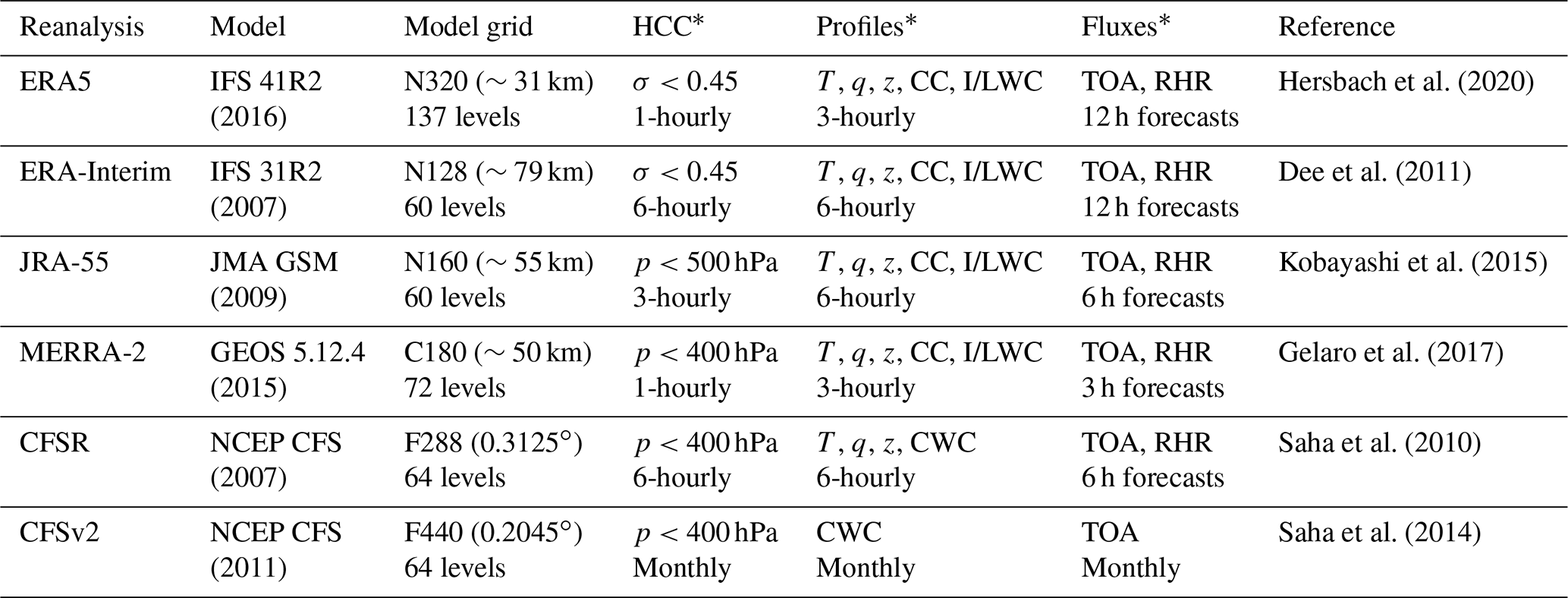
* Climatological means of HCC, CC, CWC (or I/LWC), and TOA fluxes from all reanalyses are calculated from monthly-mean products.
The full intercomparison period covers January 1980 through December 2014 and includes all five reanalyses. We also conduct a more detailed intercomparison of daily co-variations among selected variables from January 2001 to December 2010. Results for the full intercomparison are presented in Sects. 3, 4, and 6, while results based on daily co-variability are presented in Sects. 4 and 5. Our intercomparison period includes the CFSR–CFSv2 transition in January 2011 and the intermediate year 2010 (as discussed by Fujiwara et al., 2017, among others). We show in Sect. 6 that both transitions involved changes in the cloud fields that were much larger than the discontinuities at other production stream transitions. The January 2011 transition to CFSv2 also involved changes in the atmospheric-model formulation governing interactions between clouds and radiation. A brief summary of differences in tropical cloud and radiation fields between CFSR and CFSv2 is provided in Appendix B.
2.2 Observational data
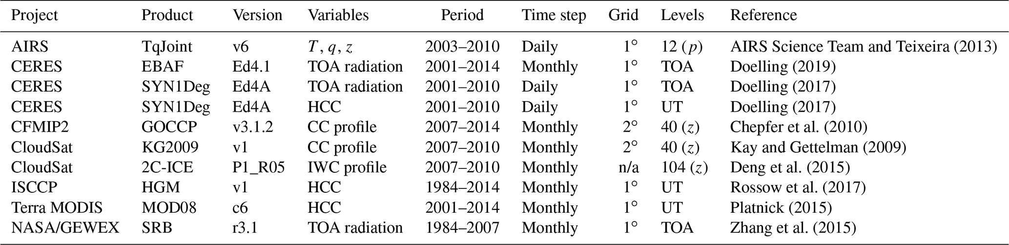
We use several observationally based data products to supply context, including TOA radiative fluxes, cloud fraction, cloud ice water content, and atmospheric thermodynamic state variables (Table 2). Observations of these variables are subject to a number of uncertainties, including lack of sensitivity to optically thin clouds or clouds composed of small particles (e.g. Dessler and Yang, 2003), uncertainties caused by overlapping cloud layers (e.g. Zhang et al., 2005), errors in cloud top height (e.g. Sherwood et al., 2004), and diurnal or spatial sampling biases (e.g. Fowler et al., 2000; Hearty et al., 2014). As our primary focus is on the intercomparison of reanalysis products, we have not applied a satellite cloud observation simulator (e.g. Bodas-Salcedo et al., 2015; Stengel et al., 2018) to the reanalysis outputs. Use of a satellite simulator could address sensitivity and sampling biases for easier comparison with observations; however, it could also obscure inter-reanalysis differences in cloud types that are not well observed and complicate analysis of cloud radiative effects in each reanalysis. Accordingly, comparisons between reanalysis products and satellite cloud observations in this paper should be interpreted with care.
AIRS Science Team and Teixeira (2013)Doelling (2019)Doelling (2017)Doelling (2017)Chepfer et al. (2010)Kay and Gettelman (2009)Deng et al. (2015)Rossow et al. (2017)Platnick (2015)Zhang et al. (2015)Table 2Summary of observational data sets, listed in alphabetical order by project. TOA stands for the top of the atmosphere, and UT stands for upper troposphere, where the latter comprises pressures less than 500 hPa for CERES SYN1Deg and pressures less than 440 hPa for ISCCP and MODIS. Other abbreviations are defined in the text. n/a: not applicable.
The International Satellite Cloud Climatology Project (ISCCP) has produced observationally based descriptions of clouds and their attributes using geostationary and polar-orbiting satellite measurements (Rossow and Schiffer, 1991). We use the H-series Global Monthly (HGM) product for January 1984–December 2014 (Rossow and Schiffer, 1999; Rossow et al., 2017). As a supplement to the ISCCP cloud data, we use all-sky and clear-sky fluxes of long-wave (LW) radiation at the TOA from the NASA Global Energy and Water Cycle Experiment (GEWEX) Surface Radiation Budget (SRB) project covering January 1984 through December 2007 (Stackhouse et al., 2011; Zhang et al., 2015). These data are based on radiative calculations that combine observed fluxes and ozone with Goddard Earth Observing System Data Assimilation System, Version 4 (GEOS-4) analyses of temperature and water vapour. Pixel-level data from ISCCP are used to estimate cloud radiative effects in SRB.
We use several products from the Clouds and the Earth's Radiant Energy System (CERES) experiment (Wielicki et al., 1996). First, we use time-mean TOA fluxes calculated from Energy Balanced and Filled (EBAF) monthly-mean products at 1∘ × 1∘ spatial resolution (Doelling, 2019). We use CERES EBAF Edition 4.1, which provides clear-sky TOA fluxes that are specifically intended for comparison with model outputs (Loeb et al., 2020). Second, we use daily-mean Synoptic Radiative Fluxes and Clouds (SYN1Deg) products at 1∘ × 1∘ spatial resolution (Doelling, 2017). The SYN1Deg data set represents an intermediate step in the production of the monthly EBAF data set. SYN1Deg provides several estimates of TOA radiative fluxes, including direct measurements, outputs from initial “untuned” radiative transfer model simulations, and outputs from a second set of radiative transfer simulations in which the model input variables are adjusted to bring the simulated fluxes into better agreement with the observed fluxes. The initial atmospheric state for radiative computations is taken from the GEOS-5 data assimilation system, a different version of that used for MERRA-2. Only the final adjusted fluxes are discussed, as these products are most appropriate for computing cloud radiative effects for comparison with reanalysis estimates. The results are qualitatively similar when the direct measurements are used instead. Along with TOA radiative fluxes, the SYN1Deg data set includes estimates of cloud fraction retrieved using measurements collected by the Moderate-Resolution Imaging Spectroradiometer (MODIS) and geostationary satellites (Minnis et al., 2011; Doelling et al., 2013). We also use high-cloud fraction (HCC) data from Collection 6 of the Terra MODIS Level 3 Atmosphere Product (MOD08; Platnick, 2015).
For observations of the thermodynamic state of the atmosphere, we use level 3 data from the Atmospheric Infrared Sounder (AIRS) version 6 “TqJoint” collection (AIRS Science Team and Teixeira, 2013). This data set provides gridded representations of temperature, moisture, and other fields based on a consistent set of initial retrievals in each grid cell (Tian et al., 2013). As the finest temporal resolutions of other data examined in this study are daily means, we average data from ascending and descending passes together. Variables taken from AIRS TqJoint include temperature, water vapour mass mixing ratio, and geopotential height between January 2003 and December 2014.
Finally, we examine three products derived from CloudSat and Cloud-Aerosol Lidar and Infrared Pathfinder Satellite Observation (CALIPSO) measurements. These include two monthly estimates of cloud fraction vertical profiles, one based on combined information from CloudSat and CALIPSO (Kay and Gettelman, 2009) and one based on CALIPSO alone (Chepfer et al., 2010). We use the combined CloudSat–CALIPSO product for the 4 years of 2007–2010 and the GCM-Oriented CALIPSO Cloud Product (general circulation model; GOCCP) for the 8 years of 2007–2014. The first product was discontinued after CloudSat switched to sunlit-only observations in early 2011. We also use ice water content (IWC) measurements from CloudSat and CALIPSO based on the 2C-ICE (CloudSat and CALIPSO Ice Cloud Property Product) retrieval algorithm (R05; Deng et al., 2015), averaged for all tropical profiles (10∘ S–10∘ N) over 2007–2010. CloudSat- and CALIPSO-based data sets are provided on height grids, which we convert to pressure using the barometric equation with a constant scale height of 7.46 km. This approach introduces uncertainty in the precise vertical location (in pressure coordinates) of features observed by CloudSat and CALIPSO, which should be taken into consideration when comparing these features to those produced by the reanalyses.
2.3 Derived variables and statistical treatments
Variables directly related to tropical high clouds include HCC and vertical profiles of cloud fraction and cloud water content, while variables used to explore the impacts of differences in high clouds include TOA radiative fluxes and vertically resolved radiative heating rates within the upper troposphere, tropopause layer, and lower stratosphere. All vertically resolved variables are evaluated on pressure levels, interpolated from height or model levels when necessary.
Cloud radiative effects (CREs) are computed as clear-sky minus all-sky fluxes using positive-upward fluxes at the TOA so that LWCRE (long-wave) is generally positive (the presence of clouds reduces outgoing long-wave radiation – OLR) and SWCRE (short-wave) is generally negative (the presence of clouds increases the planetary albedo). CREs are sensitive to differences in both all-sky and clear-sky fluxes (e.g. Soden et al., 2004); accordingly, we report differences in both all-sky and clear-sky TOA fluxes below.
Variables used to diagnose the potential origins of differences in high clouds include SST; vertical velocity at 500 hPa; and vertical profiles of temperature, specific humidity, and geopotential height between 1000 and 100 hPa. The latter three variables are used to compute moist static energy:
where g is gravitational acceleration in Earth's lower atmosphere, z is geopotential height, cp is the specific heat capacity for dry air, T is temperature, Lv is latent enthalpy of vapourization at 0 ∘C, and q is specific humidity. Temperature and specific humidity are also used to calculate equivalent potential temperature (θe), which is then used to diagnose the potential instability of the lower troposphere as the difference in equivalent potential temperature between the lower troposphere (850 hPa) and the middle troposphere (500 hPa):
Equivalent potential temperature is computed according to the formula proposed by Bolton (1980) using the MetPy software package (May et al., 2008–2020). Relative humidity (RH) is calculated with respect to liquid water using MetPy. This approach avoids inconsistencies in the implementation of the liquid–ice transition among the different data sets (see Appendix A1). Ratios between saturation vapour pressures with respect to ice and with respect to liquid water are calculated using the empirical formulas suggested by Emanuel (1994).
The level of zero radiative heating (LZRH) is determined for all profiles for which the daily-mean net radiative heating rate is positive at 100 hPa. All-sky total radiative heating rates (LW + SW; short-wave) are linearly interpolated onto a 1000-level grid between 100 and 500 hPa with equal spacing in ln (p). The LZRH is then defined as the largest pressure for which all net radiative heating rates are positive between 100 hPa and that level (inclusive).
Statistical treatments mainly consist of composite averages or distributions conditioned on ranked quartiles of LWCRE (i.e. four bins separated by the 25th percentile, the median, and the 75th percentile). We focus in particular on the largest values of LWCRE (denoted as Q4) in the inner tropics (10∘ S–10∘ N) as a proxy for strong convective activity. Results are very similar for ranked quartiles of all-sky OLR, with OLR reversed so that Q4 corresponds to the smallest values of OLR. Using HCC instead of LWCRE produces more substantial differences, particularly for MERRA-2. Given discrepancies in the precise definition of HCC across reanalyses (Table 1) and the difficulty of defining an appropriate observational benchmark for HCC, we judge HCC less suitable for this purpose. We select LWCRE rather than OLR for convenience of presentation. Averages taken in the horizontal dimension are weighted by relative area; 2-dimensional kernel density estimates are computed using the k-dimensional tree-based implementation in scikit-learn (Pedregosa et al., 2011) with a Gaussian kernel. Optimal bandwidths for kernel density estimates are identified using a 20-fold grid-search cross-validation on randomly selected subsets of the data and consistently converge to values near 1 (0.8–1.3) for LWCRE and values near 2 (1.5–2.4) for SWCRE.
Figure 1 shows the time-mean distributions of high-cloud fraction (HCC) in the tropics based on ISCCP HGM observationally based analysis and the five individual reanalyses for 1984–2014. Area-weighted mean values of HCC averaged over the tropics (30∘ S–30∘ N) are noted for each product. The definition of HCC varies somewhat among these data sets, with the lower bound of the high-cloud layer ranging from 500 to 400 hPa (Tables 1 and 2). We show below (Fig. 3) that reanalysis-derived cloud fraction profiles have minima between 400 and 500 hPa in the tropics so that differences in the precise definition of HCC should not greatly impact qualitative comparisons based on Fig. 1.
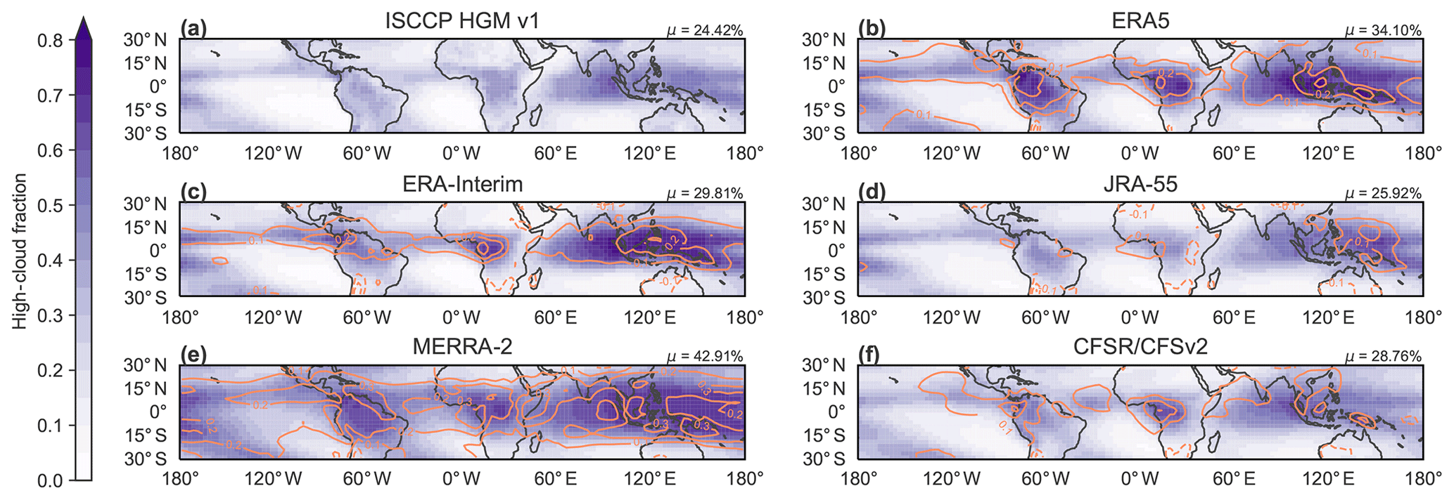
Figure 1Climatological mean spatial distribution of high-cloud cover (HCC) for (a) ISCCP HGM, (b) ERA5, (c) ERA-Interim, (d) JRA-55, (e) MERRA-2, and (f) CFSR/CFSv2 over 1984–2014. Differences relative to ISCCP HGM are shown for each reanalysis as orange contours (dashed for negative values) at intervals of 0.1. The area-weighted tropical-mean (30∘ S–30∘ N) HCC based on each product is shown at the upper-right corner of the corresponding panel.
Tropical-mean HCCs among the reanalyses are smallest in JRA-55 and largest in MERRA-2. For JRA-55, differences relative to the other reanalyses are most pronounced over canonical deep convective regions, including the tropical eastern Indian Ocean, equatorial Africa, and the Maritime Continent. By contrast, positive biases in MERRA-2 are largest around the flanks of the deep convective regions. Tropical-mean values of HCC are similar between ERA-Interim and CFSR/CFSv2 but with substantial differences in the spatial patterns of HCC between these two reanalyses. Most notably, ERA-Interim produces larger HCCs than CFSR/CFSv2 in the deep convective regions of the tropics (especially in the Indo-Pacific region). The spatial pattern in ERA5 is similar in many ways to that in ERA-Interim but with further increases in HCC over tropical convective regions (especially over land). ERA5 has larger HCCs than ERA-Interim in tropical South America and Africa, as well as in the South Asian monsoon region, the Pacific portion of the intertropical convergence zone (ITCZ), and the South Pacific convergence zone (SPCZ). These differences contribute to an increase of 0.04 (∼14 %) in the tropical-mean HCC between ERA-Interim and ERA5. Bechtold et al. (2014) reported that changes to parameterized convection in the ECMWF atmospheric model implemented between ERA-Interim and ERA5 yielded lower biases against observed brightness temperatures in land convective regions, especially for channels sensitive to the upper troposphere. However, as differences in cloud top temperatures between the two model versions could also influence the simulated brightness temperatures, these lower biases cannot be directly attributed to improvements in HCC.
Initial comparison with ISCCP HGM suggests that the reanalyses systematically overestimate HCC, with the tropical mean from JRA-55 (25.74 %) falling closest to that from ISCCP (24.42 %). However, as discussed at the beginning of Sect. 2, direct comparisons between cloud variables derived from satellite observations and those derived from models can be misleading. MERRA-2 provides outputs from the Cloud Feedback Model Intercomparison Project (CFMIP) Observation Simulator Package (COSP; Bodas-Salcedo et al., 2015) as an ancillary product in the reanalysis. Included in this product are estimates emulating HCC as observed by MODIS. Whereas MERRA-2 produces a tropical-mean HCC of 43.35 % during 2001–2014, the MERRA-2 COSP product indicates that MODIS would observe a tropical-mean HCC of only 24.71 %. This latter estimate is in good agreement not only with ISCCP HGM but also with Terra MODIS (26.04 %) and CERES SYN1Deg (23.89 %) gridded products (Fig. 2) and extends to the spatial distribution of HCC. The largest difference between the standard MERRA-2 HCC product and the MERRA-2 COSP product is a reduction in HCC outside the canonical deep convective regions of the tropics. This difference suggests that the large HCCs produced by MERRA-2 in these areas are associated with optically thin clouds having small water paths, which cannot be readily observed by MODIS. The close agreement between MERRA-2 COSP and observational estimates does not necessarily mean that the larger HCCs in MERRA-2 are more realistic (i.e. that the other reanalyses substantially underestimate HCC in the tropics). Rather, it indicates only that MERRA-2 produces a reasonably realistic distribution of the high clouds that can be readily observed by passive infrared instruments like MODIS. A recent study in which a cloud simulator was applied to ERA-Interim outputs also indicates good agreement with observed HCCs in the tropics, with a slight positive bias in the inner-tropical regions (Stengel et al., 2018).
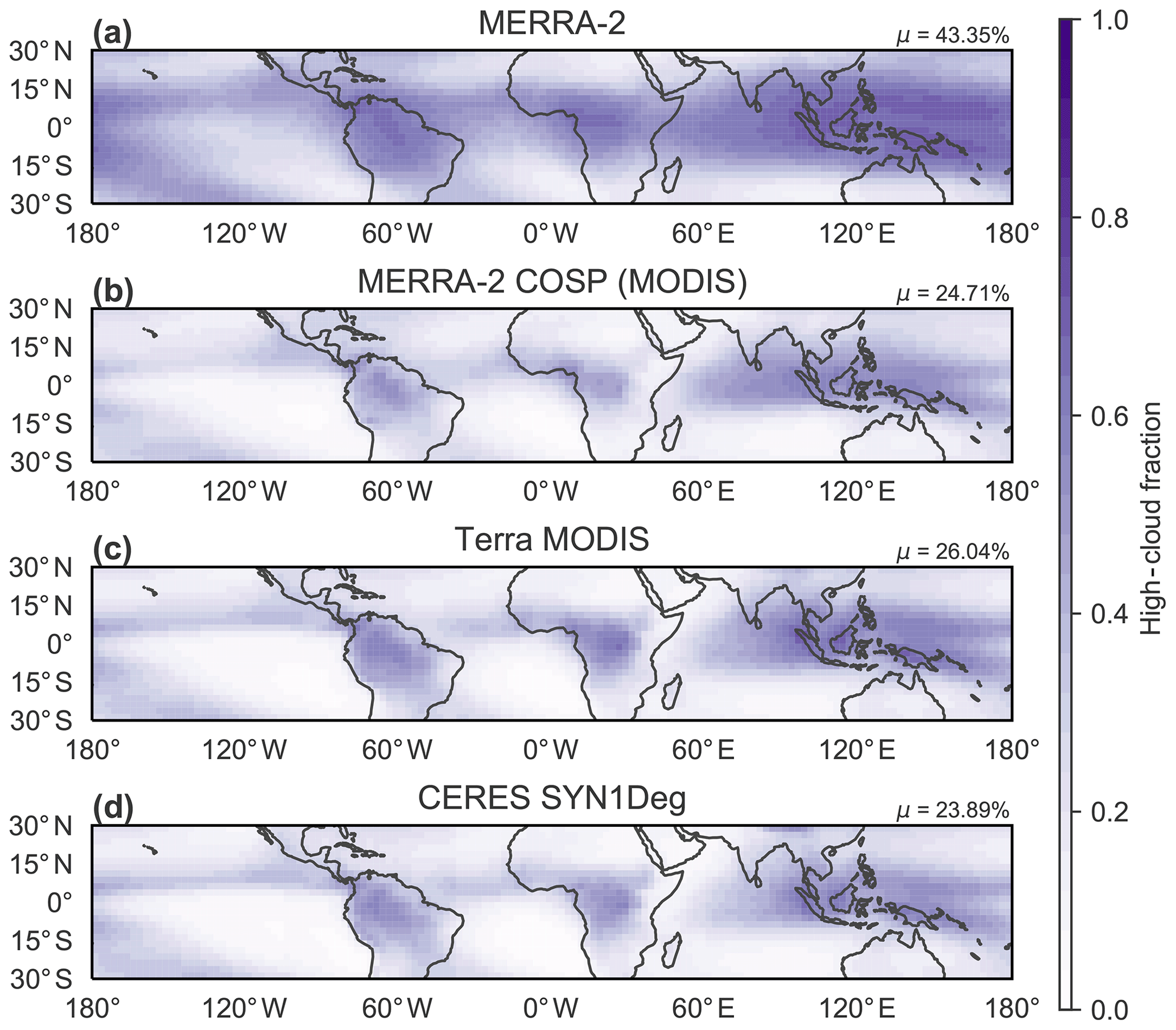
Figure 2As in Fig. 1a but for (a) direct output from MERRA-2, (b) MERRA-2-COSP (emulating MODIS observations of the MERRA-2 atmosphere), (c) Terra MODIS, and (d) CERES SYN1Deg (based primarily on Terra and Aqua MODIS) for 2001–2014. The area-weighted tropical-mean (30∘ S–30∘ N) high-cloud cover based on each product is shown at the upper-right corner of the corresponding panel.
Figure 3 shows time-mean zonal-mean profiles of cloud fraction in the tropical upper troposphere as functions of latitude and pressure. ERA5, ERA-Interim, JRA-55, and MERRA-2 all show maxima in cloud fraction near the base of the tropical tropopause layer. The peak value in ERA-Interim is centred at 150 hPa, slightly above that in ERA5 (∼175 hPa) and MERRA-2 (∼200 hPa) and slightly below that in JRA-55 (∼125 hPa). JRA-55 also shows a secondary maximum near 200 hPa. All of these maxima are most pronounced in the Northern Hemisphere between 5 and 10∘ N, reflecting the preferred position of the intertropical convergence zone (ITCZ). CFSR does not provide vertical profiles of cloud fraction and is therefore not represented in Fig. 3.
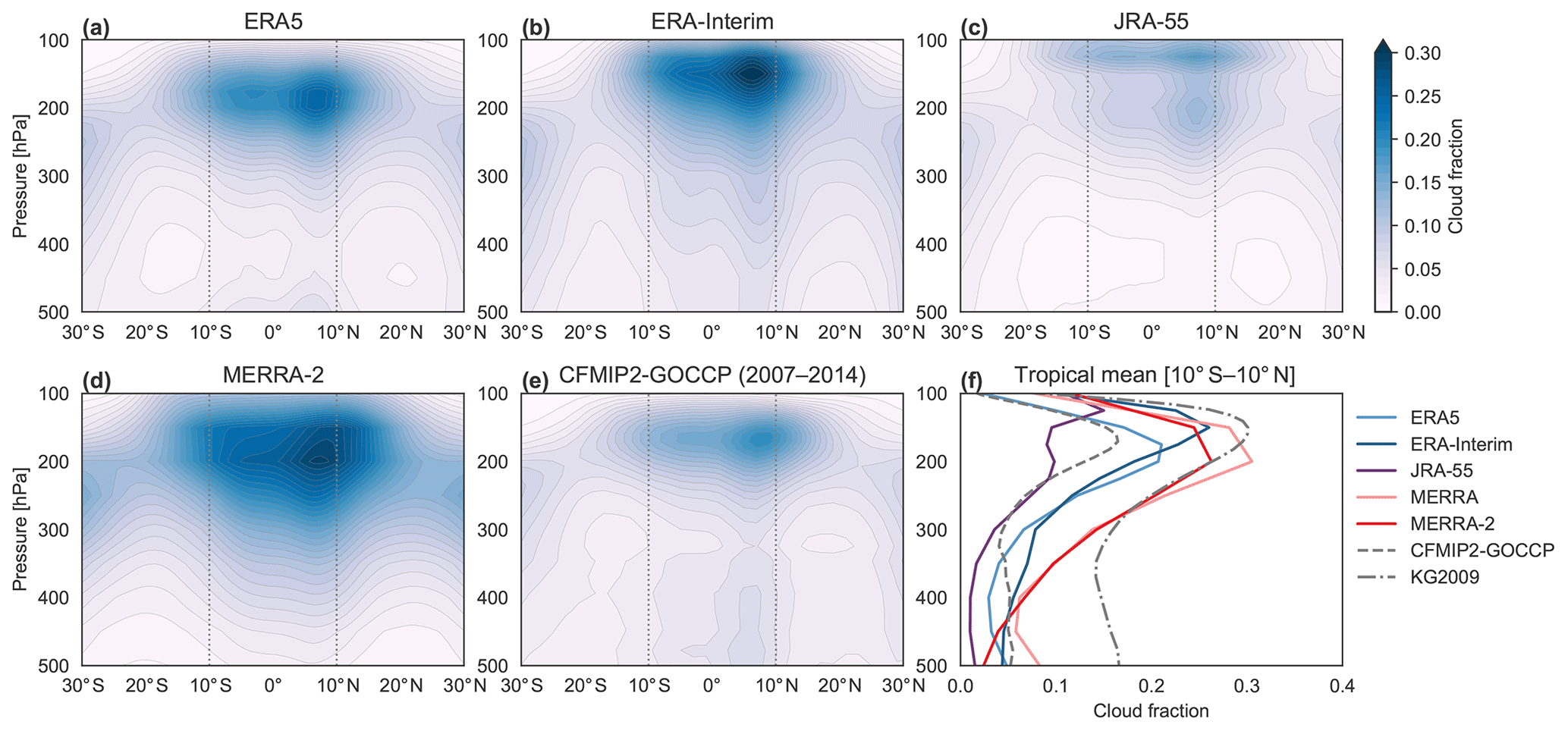
Figure 3Time-mean zonal-mean distributions of cloud fraction based on the (a) ERA5, (b) ERA-Interim, (c) JRA-55, and (d) MERRA-2 reanalyses (1980–2014), along with (e) an observationally based distribution from the GOCCP CALIPSO-based product produced for CFMIP2 (Chepfer et al., 2010), which covers 2007–2014. Inner-tropical-mean (10 ∘S–10∘ N) profiles of cloud fraction based on these five estimates are shown in (f), along with profiles from MERRA and the combined CloudSat–CALIPSO product derived by Kay and Gettelman (2009). The latter is averaged over 2007–2011. Vertical lines in (a) through (e) mark the bounds of the averaging domain. CFSR does not provide vertical profiles of cloud fraction.
Observationally based estimates of vertically resolved cloud fraction from CALIPSO (CFMIP2-GOCCP; Chepfer et al., 2010) are shown in Fig. 3e and f, with a tropical-mean profile based on CloudSat and CALIPSO (KG2009; Kay and Gettelman, 2009) also included in Fig. 3f. The zonal-mean distribution based on KG2009 is qualitatively similar to that based on CFMIP2-GOCCP and is therefore omitted from Fig. 3; however, these two data sets show large differences in the magnitude of cloud fraction within the tropical upper troposphere (Fig. 3f). The range of cloud fractions spanned by the two observationally based estimates is comparable to that spanned by the reanalysis products. Like the reanalyses, the observational products indicate that the maximum cloud fraction is located in the Northern Hemisphere tropics. The vertical placement of this maximum is around 150–175 hPa, between that produced by ERA-Interim and that produced by ERA5. This indicates that the altitude of the maximum in MERRA-2 is slightly too low, a known issue in the GEOS-5 model. The bimodal structure of the cloud fraction profile and the extremely high altitude of the peak values (125 hPa) are unique to JRA-55. Together with the relatively small values of HCC in JRA-55 (Fig. 1e), we conclude that this reanalysis underestimates high-cloud fractions through most of the tropical upper troposphere. The observational estimates also include secondary maxima in cloud fraction between 400–500 hPa, while most of the reanalyses produce local minima in this region. This difference suggests that the reanalysis models may systematically underestimate the depth, frequency, or amount of cloud detrained by cumulus congestus in the tropics (Johnson et al., 1999).
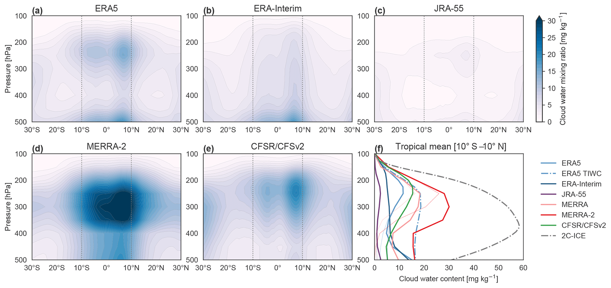
Figure 4Time-mean zonal-mean distributions of total cloud water content based on the (a) ERA5, (b) ERA-Interim, (c) JRA-55, (d) MERRA-2, and (e) CFSR/CFSv2 reanalyses (1980–2014). Inner-tropical-mean (10∘ S–10∘ N) profiles based on these five reanalyses are shown in (f), along with profiles from MERRA and an observationally based estimate of total ice water content (cloud ice + snow) during 2007–2010 from the CloudSat–CALIPSO 2C-ICE product. Vertical lines in (a) through (e) mark the bounds of the averaging domain. Dashed lines in (f) indicate ice-only water contents from the reanalyses that provide this information (all but CFSR/CFSv2). The total ice (TIWC; cloud ice + snow) profile from ERA5 is also included for comparison with 2C-ICE.
Differences among the reanalyses are even more pronounced with respect to time-mean zonal-mean distributions of cloud water content (CWC) in the tropical upper troposphere (Fig. 4). Here CWC represents the sum of ice and liquid water content, except for the CloudSat estimate shown in Fig. 4f, which includes only ice. Among the reanalyses, MERRA-2 (Fig. 4d) produces the largest CWCs in this region, with a pronounced peak at 300 hPa. Although MERRA-2 produces smaller cloud fractions in the tropical upper troposphere than its predecessor, MERRA (Fig. 3f), it produces substantially larger CWCs (Fig. 4f). The assumed effective radius for ice particles was reduced between MERRA and MERRA-2, along with several other changes aimed at increasing upper-tropospheric humidity in the model (Molod et al., 2012, 2015). The large CWCs in MERRA-2 have significant impacts on radiative transfer (see Sect. 4). CFSR/CFSv2 (Fig. 4e) produces a similarly pronounced vertical maximum in CWC but shifted slightly higher in altitude and with a peak magnitude (15.4 mg kg−1 at 250 hPa) roughly half that produced by MERRA-2 (30.1 mg kg−1 at 300 hPa) when averaged over the inner tropics (10∘ S–10∘ N). JRA-55 (Fig. 4c) shows a qualitatively similar distribution to those of MERRA-2 and CFSR/CFSv2 but with much smaller magnitudes (maximum value: 2.4 mg kg−1 at 250 hPa). This difference is again consistent with JRA-55 underestimating cloud cover in the tropical upper troposphere. The zonal-mean distribution of CWC in ERA-Interim (Fig. 4b) is remarkably different from that in the other reanalyses, including ERA5 (Fig. 4a), with no distinct maximum in the tropical upper troposphere. Instead, ERA-Interim shows a monotonic decrease in CWC with increasing altitude above 500 hPa. Although it is difficult to pinpoint the reason for the difference in vertical profiles of CWC between ERA-Interim and ERA5, changes to the treatment of entrainment and detrainment in the convective scheme (Appendix A2) may contribute. These changes, together with improvements in prognostic microphysics, alter the structure of the convective mass flux and improve coupling between convection and the tropical environment (Bechtold et al., 2008, 2014).
The tropical-mean profile of IWC based on the CloudSat 2C-ICE product between 2007 and 2010 is shown for context in Fig. 4f. The diurnal sampling of CloudSat along its initial orbit in the A-Train constellation (Equator-crossing times around 01:30 and 13:30 LST – local solar time) should be taken into account when comparing the CloudSat profile to the reanalyses, as this orbit misses the late-afternoon peak of continental convective activity in the tropics (e.g. Yang and Slingo, 2001). It is also important to note that the CloudSat estimate represents total IWC, including both precipitating and cloud ice. We may therefore expect the profile maximum to be both larger in magnitude and lower in altitude than one based on cloud ice alone (Li et al., 2012, 2016). This expectation is supported by Fig. 4f, as the peak value of IWC based on CloudSat is larger and lower in altitude relative to the reanalysis profiles (54.2 mg kg−1 at ∼370 hPa). Despite this difference, the structure of the CloudSat profile is qualitatively more consistent with the pronounced anvil layers in ERA5, MERRA-2, and CFSR/CFSv2 than with JRA-55 or ERA-Interim.
The cumulus congestus peak in the middle troposphere that does not appear in reanalysis estimates of cloud fraction (but does appear in observations) is evident in the reanalysis estimates of CWC but not in the CloudSat estimate. The latter may be attributable to the exclusion of liquid water from the CloudSat estimate, although previous analyses of CloudSat CWCs did not show a clear maximum here even when the liquid phase was included (see, e.g. Su et al., 2011). MERRA-2, ERA-Interim, ERA5, and JRA-55 all indicate large liquid water fractions in clouds at these altitudes. In ERA-Interim, 12.5 % of cloud water at 400 hPa averaged over the inner tropics is liquid, rising to 63.3 % at 500 hPa. These ratios are larger in ERA5 (28.6 % and 86.0 %, respectively) and MERRA-2 (86.4 % and 99.8 %) and smaller in JRA-55 (3.3 % and 60.4 %). CFSR does not provide separate outputs for liquid and ice water contents. The prevalence of liquid water content at these altitudes in MERRA and MERRA-2 relative to CloudSat is a known feature of the GEOS-5 data assimilation system (Su et al., 2011).
4.1 Top-of-atmosphere radiation budget
Figure 5 shows spatial distributions of all-sky and clear-sky OLR based on CERES EBAF during 2001–2014, along with differences between the five individual reanalysis products and CERES. Rather than direct observations (with clear-sky fluxes taken only from cloud-free columns), the CERES EBAF fluxes discussed in this section are estimates for the entire column with clouds removed and are suitable for direct comparison with model-generated clear-sky fluxes (Loeb et al., 2020). CERES EBAF estimates a time-mean tropical-mean OLR of 260.3 W m−2 over 2001–2014, smaller than in any of the reanalyses except for MERRA-2. Better agreement is found for clear-sky OLR, with tropical-mean values from all reanalyses within ±2.5 W m−2 of the CERES EBAF estimate. Accordingly, the time-mean tropical-mean LWCRE based on CERES EBAF (27.3 W m−2) was larger than that produced by any of the reanalyses except for MERRA-2 (31.6 W m−2). ERA-Interim, ERA5, and CFSR/CFSv2 underestimate clear-sky OLR even as they overestimate all-sky OLR so that negative biases in the tropical-mean LWCRE are approximately twice as large as positive biases in tropical-mean OLR in each of these three reanalyses. Comparison with observationally based estimates with longer durations further indicates that most of the reanalyses overestimate OLR and underestimate LWCRE in the tropics. NASA/GEWEX SRB indicates tropical-mean values of 259.4 W m−2 for all-sky OLR and 27.7 W m−2 for LWCRE over 1984–2007, while the NOAA Interpolated OLR product indicates a tropical-mean value of 250.7 W m−2 for all-sky OLR over 1980–2014.

Figure 5Climatological mean spatial distributions of all-sky outgoing long-wave radiation (OLR; shading) and clear-sky outgoing long-wave radiation (CLR; contours at intervals of 10 W m−2) for (a) CERES EBAF over 2001–2014. Differences relative to CERES EBAF for the same period are shown for (b) ERA5, (c) ERA-Interim, (d) JRA-55, (e) MERRA-2, and (f) CFSR/CFSv2 (abbreviated CFSR/v2). Contours in (c) through (f) cover the range within ±10 W m−2 at intervals of 4 W m−2. Tropical-mean (30∘ S–30∘ N) values of OLR and CLR based on each product are shown at the upper-right and upper-left corners, respectively, of the corresponding panel. Tropical-mean values for the long-wave cloud radiative effect (LWCRE = CLR − OLR) are listed above those for OLR.
Many differences among the reanalyses indicate an inverse relationship between relative biases in OLR and those in HCC. For example, JRA-55, which has the smallest HCCs in the tropics among the reanalyses, likewise produces the largest tropical-mean OLR and the smallest tropical-mean LWCRE. Conversely, MERRA-2, with the largest HCCs among the reanalyses, produces the smallest tropical-mean OLR and the largest tropical-mean LWCRE. ERA5 produces a slightly smaller OLR and a slightly larger LWCRE than ERA-Interim and again shows maximum differences over tropical land areas with strong convection. As with HCC, ERA-Interim and CFSR/CFSv2 produce similar tropical-mean values of both OLR and LWCRE (within ±0.5 W m−2). Most differences between these two reanalyses obey the same type of inverse relationship: ERA-Interim produces smaller values of OLR in the Indo–Pacific domain (consistent with larger HCCs in this region), while CFSR/CFSv2 produces smaller values of OLR over tropical mountain ranges (consistent with relatively large HCCs in these locations). There are some notable exceptions though, such as over Africa. ERA-Interim produces slightly larger HCCs in this region (Fig. 1), but CFSR produces smaller values of OLR (this difference is mitigated somewhat in CFSv2; cf. Fig. B2g). This type of inconsistency, in which biases in HCC and OLR do not align with simple expectations, may reflect systematic differences in the depth of convection (and thus cloud top temperature) or the water paths associated with convective anvil clouds. Although we do not directly evaluate differences in cloud top height here (owing in part to the lack of vertically resolved cloud fraction profiles in CFSR/CFSv2), we note that CFSR/CFSv2 produces a more pronounced peak in cloud water content extending to relatively higher altitudes than ERA-Interim in the tropical mean (Fig. 4f).
Figure 6 shows spatial distributions of all-sky net radiation based on CERES EBAF and the five reanalyses, with positive values indicating time-mean energy fluxes into the tropical climate system. Mean values across the tropics are positive (incoming solar radiation exceeds OLR), as indicated here by CERES EBAF (net gain of 45.0 W m−2). This excess of incoming energy in the already energy-rich tropics is essential to the “heat engine” model of the atmospheric circulation and is contributed primarily by imbalances in the clear-sky fluxes (e.g. Stephens and L'Ecuyer, 2015, and references therein). Net clear-sky fluxes into the tropics are typically somewhat larger in the reanalyses than in CERES, with overestimates as large as 7 W m−2 (in ERA-Interim). The closest match in the tropical mean is provided by JRA-55, which is within 0.1 W m−2 of CERES (this good agreement does not extend to the all-sky net radiation flux, as detailed below). Cloud effects reduce the energy excess provided by clear-sky radiation, as the negative SWCRE outweighs the positive LWCRE. However, most of the reanalyses greatly overestimate the magnitude of this reduction relative to CERES. Such overestimates have implications for atmospheric energy transport and could result at least in part from the lack of two-way coupling between cloud fields and SST in the reanalyses (e.g. Kolly and Huang, 2018; Wall et al., 2019). For JRA-55, which overestimates the net CRE by 22.5 W m−2 relative to CERES, a little more than half of the bias in the net CRE is attributable to the bias in LWCRE. The remainder is due to overestimated cloud albedo effects. Similar ratios hold for ERA5 and ERA-Interim, with biases in LWCRE contributing approximately 55 % of the overall biases in each case. For MERRA-2, overestimated cloud albedo effects more than compensate for the stronger LWCRE, producing a net CRE similar to that in ERA5 (approximately 9 W m−2 stronger than that from CERES). CFSR/CFSv2 produces a net CRE very similar to that indicated by CERES, implying compensating biases in SWCRE and LWCRE. However, the horizontal gradients of net radiation are much sharper in this reanalysis than in any of the other data sets included in Fig. 6.
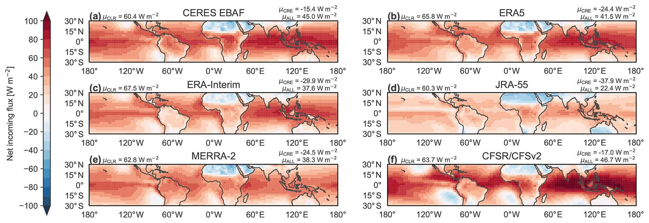
Figure 6Climatological mean spatial distributions of all-sky net incoming radiation (ALL; shading) for (a) CERES EBAF, (b) ERA5, (c) ERA-Interim, (d) JRA-55, (e) MERRA-2, and (f) CFSR/CFSv2 during 2001–2014. Tropical-mean (30∘ S–30∘ N) values of ALL and clear-sky net incoming radiation (CLR) based on each product are shown at the upper-right and upper-left corners, respectively, of the corresponding panel. Tropical-mean values for the net cloud radiative effect (CRE = CLR − ALL) are listed above those for ALL.
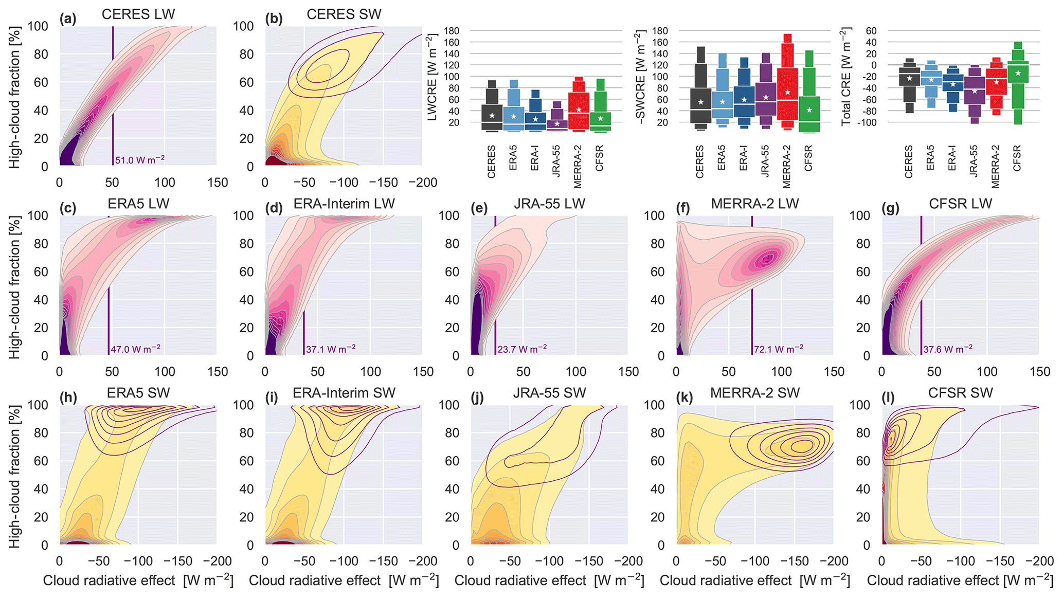
Figure 7Joint distributions of daily-mean HCC against (a) LWCRE and (b) SWCRE based on CERES SYN1Deg using gridded data from 2001 to 2010. Corresponding joint distributions are shown for (c, h) ERA5, (d, i) ERA-Interim, (e, j) JRA-55, (f, k) MERRA-2, and (g, l) CFSR. The 75th percentile of LWCRE is marked in (a) and (c–g). Sub-distributions of HCC against SWCRE associated with the values of LWCRE that exceeded the corresponding 75th percentile threshold are then shown as purple contours in (b) and (h–l). Distributions of LWCRE, SWCRE, and total CRE are shown in the upper right (in which ERA-Interim is abbreviated ERA-I), with SWCRE multiplied by −1 for convenience of presentation. The thickest boxes mark the interquartile ranges, with the medians marked as horizontal lines and the means marked as stars. The narrower extended boxes indicate the 5th, 10th, 90th, and 95th percentiles.
Relationships between tropical HCC and TOA radiation fluxes are examined in more detail in Fig. 7, which shows joint distributions of HCC against the LW and SW cloud radiative effects. The joint distributions shown in Fig. 7 are 2-dimensional frequency distributions analogous to scatterplots, where the shading indicates the density of the points and outliers are omitted. The data used to construct these distributions are daily-mean gridded values within 10∘ S–10∘ N during the period 2001–2010 and thus reflect both spatial and temporal covariability of TOA radiative fluxes and HCC. For this and other analyses that do not span the CFSR/CFSv2 transition (1 January 2011), we omit any reference to CFSv2 and refer to this reanalysis only as CFSR. Data have been interpolated when necessary to 1∘ × 1∘ spatial grids. The abscissa is reversed for plots of SWCRE so that larger absolute magnitudes of both LWCRE and SWCRE are located toward the right. Distributions of daily-mean gridded values of LWCRE, SWCRE, and total CRE are included at the upper right of Fig. 7.
The joint distribution of HCC against LWCRE based on CERES SYN1Deg indicates a tight, nearly linear relationship between these two variables, in which a large value of HCC corresponds to a large LWCRE. The 75th percentile value of LWCRE based on CERES SYN1Deg is 51.0 W m−2, which corresponds to an HCC of roughly 0.57. Among the reanalyses, CFSR is most similar to CERES SYN1Deg in its joint distribution of HCC against LWCRE. However, the CFSR distribution has a stronger curvature so that the 75th percentile of LWCRE corresponds to a smaller value of LWCRE (37.6 W m−2) despite a similar value of HCC (0.58). JRA-55 has the smallest 75th percentile value of LWCRE (23.7 W m−2). This value of LWCRE corresponds to an HCC value of around 0.56 in JRA-55, whereas it corresponds to an HCC of only 0.27 in CERES SYN1Deg, implying that the relatively small mean HCC in JRA-55 is not the only reason behind relatively weak LWCRE in this reanalysis. Joint distributions based on ERA5, ERA-Interim, and MERRA-2 are qualitatively more distinct, with secondary modes at large values of LWCRE. In ERA-Interim, there is a clear distinction in both variables between the primary mode (associated with small values of both HCC and LWCRE) and the secondary mode (associated with large values of HCC and LWCRE). HCCs associated with the latter mode are almost exclusively greater than 0.9. The 75th percentile value (37.1 W m−2) falls between the two modes and corresponds to an HCC of 0.65. The distribution based on ERA5 is similar to that based on ERA-Interim but with a greater fraction of the data (and greater variability) in the large-LWCRE mode. The 75th percentile value is thus substantially larger in ERA5 (47.0 W m−2) than in ERA-Interim, as is the mean cloud fraction associated with this value (0.75). Bimodality in MERRA-2 takes a different form. The first mode corresponds to small values of LWCRE. Although the peak of this distribution is at small values of HCC, this small-LWCRE mode still exhibits relatively large occurrence frequencies at values of HCC approaching 1. The mean HCC associated with this mode is around 0.35. The second mode peaks at relatively large values of both LWCRE (∼88 W m−2) and HCC (∼0.7). The 75th percentile of LWCRE (72.1 W m−2) is contained within the second mode, meaning that the large-LWCRE mode contains more than 25 % of the inner-tropical data points in MERRA-2. An LWCRE of 72.1 W m−2 corresponds to an HCC of approximately 0.68 in MERRA-2, slightly less than that associated with the same value of LWCRE in CERES SYN1Deg (0.73).
The unique bimodality of the HCC–LWCRE distribution in MERRA-2 is a consequence of the separation of cloud condensate in the prognostic cloud scheme into “large-scale” and “anvil” cloud types. Of these two types, anvil clouds are assigned higher number densities that translate into greater values of optical thickness when the radiation calculations are performed (Bacmeister et al., 2006). The model used to produce MERRA-2 also uses different procedures to relate the evolution of cloud fraction to autoconversion between the large-scale and anvil cloud types, which appears to result in relatively large values of cloud fraction persisting even as CWC declines (the small-LWCRE mode in Fig. 7f). Although the treatment of prognostic cloud fraction used in MERRA-2 is conceptually similar to that used in JRA-55 (Appendix A1), JRA-55 and MERRA-2 produce very different relationships between cloud fraction and condensate. Tuning efforts to increase the amount of cloud ice in the upper troposphere in MERRA-2 were motivated by a desire to improve OLR (recognizing that convective detrainment altitudes are too low in GEOS-5, the developers accepted overestimating cloud ice to get OLR right) and upper-tropospheric humidity (Molod et al., 2015). The anvil cloud fraction was then kept small relative to the cloud ice content to prevent a worsening of SWCRE as LWCRE was increased.
Joint distributions of HCC against SWCRE are consistent with SWCRE being less tightly linked than LWCRE to HCC in the tropics. However, large HCCs are typically associated with both large LWCREs and large SWCREs. CERES SYN1Deg and four of the five reanalyses show extensive overlap between large values of LWCRE and large values of SWCRE. CFSR is a notable exception, with large values of LWCRE often corresponding to small values of SWCRE. As a consequence, the distribution of total CRE based on CFSR is broader than that based on CERES or the other reanalyses, with the middle 90 % spanning from less than −100 W m−2 to approximately +40 W m−2. The weaker SWCRE associated with large HCCs results in a more positive total CRE on average, with the median value in CFSR close to zero. These differences can also be seen in the CFSR/CFSv2 climatology, which has sharper spatial gradients of net TOA radiation (Fig. 6f) and a smaller tropical-mean net CRE than any other reanalysis. Although LWCRE is weakest in JRA-55 among the data sets evaluated here, the tropical-mean SWCRE is larger in JRA-55 than in any data set except MERRA-2. The total CRE is thus substantially more negative in JRA-55 than in any other reanalysis (see also Fig. 6d). Fewer than 5 % of gridded values of total CRE in the tropics are positive in JRA-55. This latter statement also holds for ERA-Interim; however, greater compensation between LWCRE and SWCRE in ERA-Interim leads to a narrower distribution and a smaller negative bias in the tropical-mean total CRE relative to CERES. MERRA-2 tends to overestimate both LWCRE and SWCRE, especially for anvil clouds. However, compensation between these two biases produces a distribution of total CRE that is comparable to (though slightly broader than) that based on CERES SYN1Deg. Among the five reanalyses, ERA5 shows the closest agreement with CERES SYN1Deg across all three flavours of CRE. LWCRE in ERA5 is slightly weaker on average than that based on CERES, while SWCRE is similar on average but with a narrower distribution. The total CRE is thus slightly more negative in ERA5 than indicated by CERES, with a narrower distribution but good agreement in the mean value.
4.2 Radiative heating in the tropical UTLS
In addition to altering top-of-atmosphere radiative fluxes, differences in tropical high clouds may influence radiative heating rates locally within the UTLS. Among the reanalyses considered in this study, neither JRA-55 nor CFSR provide vertically resolved estimates of radiative heating under clear-sky conditions. To skirt this limitation, we construct composite mean profiles of radiative heating rates conditional on the four quartiles of LWCRE in an adaptation of the approach employed by Zhang et al. (2017). Figure 8 shows these composite profiles for the period 2001–2010, separated into total, LW, and SW radiative heating. Here, Q1 represents daily gridded heating rates for which LWCRE (at TOA; Fig. 7a and c–g) is in the smallest 25 % of all daily gridded values. Q2 and Q3 represent the lower-middle and upper-middle quartiles, respectively, while Q4 represents heating rates for which the associated LWCRE exceeds the 75th percentile value marked in Fig. 7. The impact of clouds on heating rates is then estimated as the difference between the Q4 and Q1 profiles. Results are very similar for ranked quartiles of all-sky OLR, with OLR reversed so that Q4 corresponds to the smallest values of OLR.
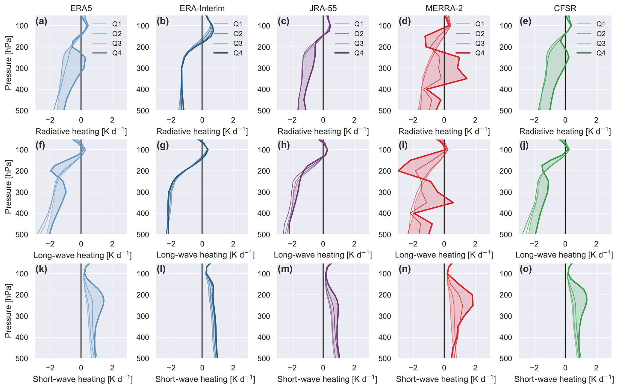
Figure 8Composite mean profiles of daily-mean radiative heating rates as a function of pressure for the first through fourth quartiles (Q1–Q4) of LWCRE in the inner tropics (10∘ S–10∘ N; see also Fig. 7) based on (a) ERA5, (b) ERA-Interim, (c) JRA-55, (d) MERRA-2, and (e) CFSR during 2001–2010. Here Q1 refers to the bottom quartile (weak long-wave CRE) and Q4 to the top quartile (strong long-wave CRE). Total radiative heating rates (upper row; a–e) are separated into (f–j) long-wave and (k–o) short-wave components in the lower two rows.
Among these five reanalyses, cloud effects on radiative heating rates are generally smallest in ERA-Interim and largest in MERRA-2. Results for these two reanalyses are consistent with those reported for ERA-Interim and MERRA by Wright and Fueglistaler (2013), who found that cloud impacts on radiative heating in MERRA are qualitatively opposite to those in ERA-Interim through much of the upper troposphere. The response in ERA-Interim is largest in the 100–200 hPa layer, where radiative heating rates are enhanced when LWCRE is large. At lower altitudes in the upper troposphere (200–400 hPa), cloud-induced increases in SW heating are effectively offset by cloud-induced increases in LW cooling. By contrast, ERA5, JRA-55, and CFSR show only weak cloud impacts on total radiative heating at pressures less than 175 hPa. In all three cases, the insensitivity in total radiative heating rates at these altitudes traces back to a near-complete compensation between enhanced LW cooling and enhanced SW heating. Substantial cloud-related perturbations in the LW and SW components extend upward to around 100 hPa in ERA5 and CFSR but only to around 150 hPa in JRA-55. MERRA-2 produces the largest cloud impacts on radiative heating rates. Indeed, direct comparison of cloud radiative effects between MERRA and MERRA-2 (not shown) indicates that cloud effects in MERRA are further amplified in MERRA-2, consistent with the increase in CWC in the tropical upper troposphere between MERRA and MERRA-2 (Fig. 4f). High-cloud effects in MERRA-2 reduce radiative heating rates in the 100–200 hPa layer (largely due to enhanced LW cooling, partially offset by enhanced SW heating) and increase radiative heating rates at pressures greater than 200 hPa. The latter results from enhanced SW heating near the top of the anvil layer (200–250 hPa) and enhanced LW heating near the base of the anvil layer (300–350 hPa), taking the MERRA-2 profile of tropical-mean cloud water content (Fig. 4f) as a guide. Cloud effects in ERA5 are intermediate between those in CFSR and MERRA-2. This is consistent with the pronounced convective anvil in the ERA5 profile of tropical-mean CWC (Fig. 4f), which better matches the profiles produced by CFSR and MERRA-2 than that produced by ERA-Interim.
Differences in the radiative impacts of tropical high clouds are linked to differences in transport through the TTL and lower stratosphere (Fueglistaler and Fu, 2006; Yang et al., 2010). Relevant metrics include the level of zero net radiative heating (LZRH) and the rate of diabatic ascent at the base of the “tropical pipe”, which defines the upward branch of the Brewer–Dobson circulation (e.g. Fueglistaler et al., 2009; Dessler et al., 2014). The LZRH marks the boundary between negative all-sky radiative heating rates (corresponding to net descent) in the tropical troposphere and positive radiative heating rates (corresponding to net ascent) in the TTL and lower stratosphere (Sect. 2.3; see also Folkins et al., 1999; Gettelman et al., 2004). To represent ascent at the base of the tropical pipe, we use the vertical velocity in potential temperature coordinates () at the 420 K isentropic level, near the top of the TTL. We evaluate distributions of LZRH pressure (Fig. 9a) and (Fig. 9b) at 420 K based on ERA5, ERA-Interim, JRA-55, MERRA-2, and CFSR during 2001–2010. Distributions conditional on the top quartile of LWCRE (Q4) for each reanalysis are shown in colour.
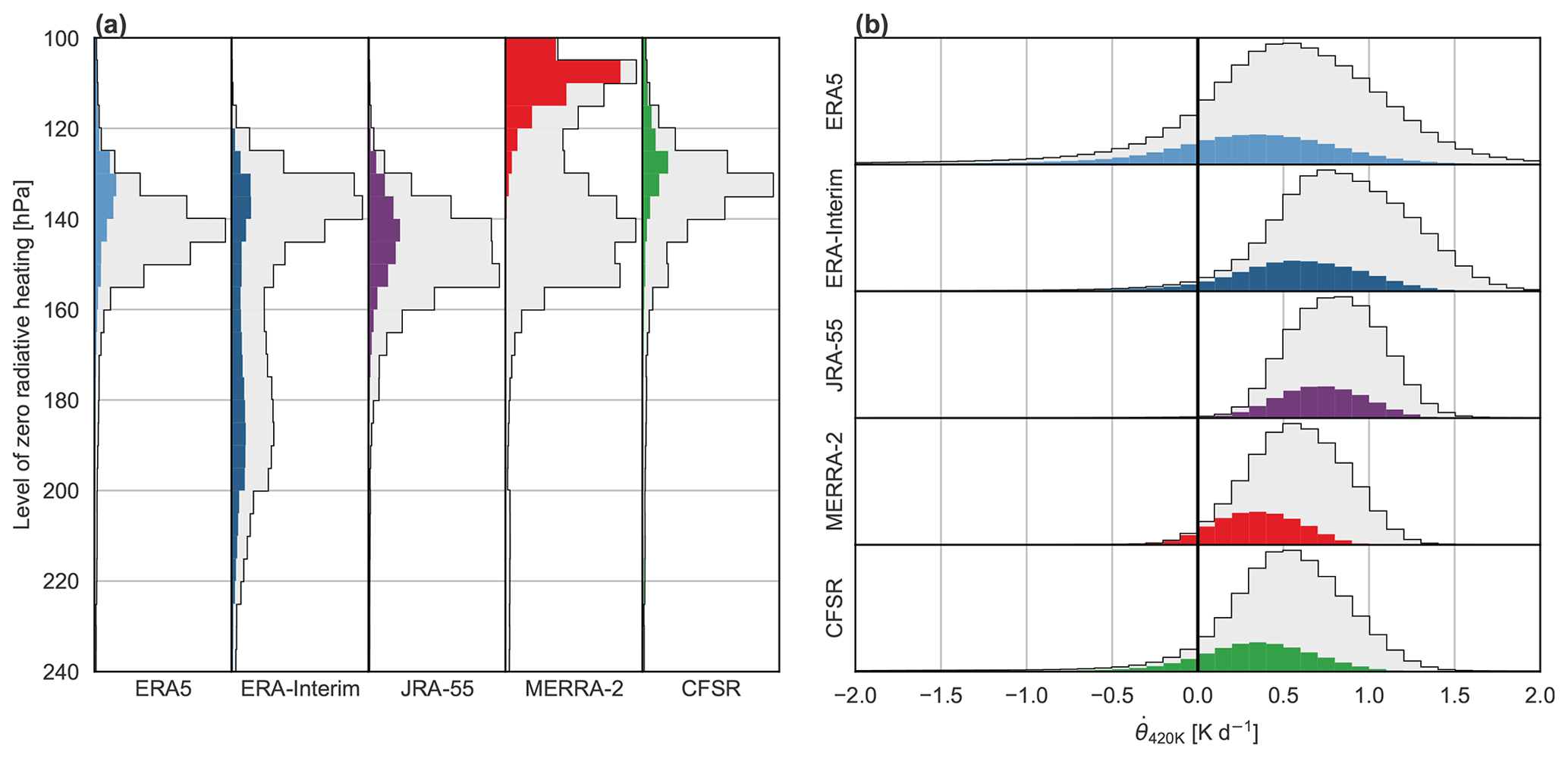
Figure 9Histograms of (a) the vertical location of the level of zero net radiative heating (LZRH) and (b) the vertical velocity in isentropic coordinates ( on the 420 K isentropic surface). Data are based on daily-mean products from (left to right and top to bottom) ERA5, ERA-Interim, JRA-55, MERRA-2, and CFSR during 2001–2010. Colour histograms show distributions for the top quartile of long-wave cloud radiative effect in each reanalysis (see Fig. 7).
The largest differences in LZRH distributions are between ERA-Interim and MERRA-2 (Fig. 9a). Neglecting the influence of clouds, the primary mode of the ERA-Interim distribution (p∼140 hPa) is located at slightly higher altitudes than that in MERRA-2 (p∼150 hPa). These primary modes match the vertical locations of the clear-sky LZRH in each system well (not shown). The more striking distinction between ERA-Interim and MERRA-2 is in the impacts of clouds on the LZRH altitude. Whereas clouds tend to lower the LZRH in ERA-Interim (to around 170 hPa on average), clouds raise the LZRH significantly in MERRA-2 (to around 110 hPa). This difference has important implications for the efficiency of mass and constituent transport from the deep convective detrainment level (200–300 hPa) into the tropical lower stratosphere. In MERRA-2, the cloudy and clear-sky modes of the distribution are almost completely distinct. By contrast, the breadth of the LZRH distribution based on ERA-Interim (and especially the breadth of the distribution associated with the largest values of LWCRE) indicates that ERA-Interim produces a broad spectrum of cloudy states. This diagnostic thus helps to clarify the environmental conditions associated with the two very different tropical-mean CWC profiles in Fig. 4f, with the pronounced anvil layer in MERRA-2 in sharp contrast to the gradual decrease of CWC with height in ERA-Interim. Distributions of the LZRH location based on ERA5, JRA-55, and CFSR are more consistent with each other. Each distribution has one major mode, although the altitude of the LZRH tends to be highest in CFSR (median: 134 hPa), followed by ERA5 (144 hPa) and JRA-55 (148 hPa). All three reanalyses indicate slight upward shifts toward lower pressures (by around 5 hPa) in the median LZRH location associated with the largest values of LWCRE, but these shifts are much less pronounced than that suggested by MERRA-2.
Distributions of at 420 K (Fig. 9b) are more consistent among the reanalyses. Differences in the mean value are consistent with previous assessments (Schoeberl et al., 2012; Abalos et al., 2015; Tao et al., 2019), with ERA-Interim (average: 0.82 K d−1) and JRA-55 (0.80 K d−1) having stronger lower-stratospheric ascent than MERRA-2 (0.56 K d−1) or CFSR (0.49 K d−1). The mean value in ERA5 (0.49 K d−1) is consistent with that in MERRA-2 and CFSR but with a much broader distribution. Our focus here is on the cloud effects and the role they play in the overall differences. All five reanalyses indicate weaker lower-stratospheric radiative heating rates in atmospheric columns with large values of LWCRE. As with many of the diagnostics examined in this study, this effect is least pronounced in JRA-55, with the mean for Q1 (smallest LWCREs) only 0.13±0.03 K d−1 larger than that for Q4 (largest LWCREs). This relatively small cloud influence may contribute to the relatively narrow distribution of in JRA-55. By contrast, the much broader distributions of in ERA5 and ERA-Interim are accompanied by large cloud effects, with differences of 0.49±0.12 K d−1 between Q1 and Q4 in ERA5 and 0.45±0.06 K d−1 in ERA-Interim. These large cloud effects reflect sharper spatial gradients in HCC (Fig. 1c) and LWCRE (Fig. 5c) between tropical deep convective regions and surrounding areas in the ECMWF reanalyses relative to JRA-55. The cloud influence on in MERRA-2 is comparable to that in ERA-Interim, with a difference of 0.39±0.03 K d−1 between Q1 and Q4. However, the distribution based on MERRA-2 is compressed toward the mean relative to that based on ERA-Interim, with fewer extreme values and shorter tails. Only 8 % of values in MERRA-2 fall outside the interval [0, 1] K d−1, as opposed to 36 % of values in ERA-Interim (33 % in ERA5). This pairing of large cloud effect and narrow distribution implies a strict stratification of lower-stratospheric heating rates with respect to LWCRE, with values of in MERRA-2 approaching those in JRA-55 as the effects of clouds are reduced. The mean difference between these two reanalyses is ∼0.4 K d−1 in Q4 (where the mean LWCRE in MERRA-2 is more than double that in JRA-55) but only ∼0.1 K d−1 in Q1 (where mean values of LWCRE are 3.1 W m−2 in both systems). Our results thus support the suggestion by Tao et al. (2019) that differences in climatological HCC in the tropics can explain much but not all of the difference in lower-stratospheric ascent rates between these reanalyses. The cloud effect on lower-stratospheric heating rates is 0.31±0.09 K d−1 in CFSR. The uncertainty is relatively large in CFSR because of large variance in distributions of within each LWCRE quartile (primarily due to higher occurrence frequencies of negative values in all four quartiles). Approximately 4 % of values associated with the relatively cloud-free Q1 and Q2 groupings in CFSR are negative, an order of magnitude larger than the fraction in ERA-Interim and several orders of magnitude larger than the fractions in JRA-55 and MERRA-2. However, the largest variance in is produced by ERA5. Although variance decreases with decreasing LWCRE, the fraction of negative values in Q1 and Q2 (9 %) is still more than double that in CFSR. The broader distribution of diabatic heating rates in this reanalysis may be related to improved consistency between diabatic and kinematic vertical motion in the lower stratosphere in ERA5 relative to ERA-Interim (Hoffmann et al., 2019).
The prognostic cloud parameterizations in the reanalysis models consider two sources of high clouds: detrainment from deep convection and in situ formation due to large-scale saturation (see Appendix A). Sinks include autoconversion of cloud water to precipitation and evaporation or sublimation of cloud water into unsaturated air. In considering the origins of differences in high clouds among the reanalyses, we therefore focus on factors that can influence the sources and sinks of high clouds or clarify coupled relationships between high clouds and their environment. With respect to the convective source, we examine relationships with SST, thermodynamic stability in the lower troposphere, grid-scale vertical velocity and RH in the middle troposphere (500 hPa), and the mean vertical profile of moist static energy (MSE). We then use relationships among CWC, RH, and radiative heating near the base of the TTL (150 hPa) and near the cold-point tropopause (100 hPa) to assess the relative balance of in situ versus convective clouds in the TTL. All relationships are assessed using daily-mean data in the inner tropics (10∘ S–10∘ N). The use of daily means collapses diurnal variations in tropical convective activity that may be poorly represented in reanalyses (e.g. Bechtold et al., 2014). Diurnal variability may imprint on relationships among daily-mean variables, but we do not explore this possibility here. We cannot fully distinguish between causes and effects. All of the variables we examine in this section are intimately connected to cloud and convection processes so that differences in these variables may indicate the causes of cloud biases, reflect the effects of those biases, or both of the above. To address this, we link differences in the examined variables to differences in model parameterizations or data assimilation procedures whenever possible. Although we cannot unequivocally tie each bias to a distinct origin of this type, this information may be helpful both for understanding differences between the reanalyses and for highlighting potential targets for improvement in the reanalysis systems.
5.1 Convection and its environment
Tropical deep convection tends to cluster over the warmest SSTs. This behaviour is captured by all five of the reanalysis systems, with the largest LWCREs systematically associated with the largest SSTs. Tropical-mean SSTs prescribed during the 2001–2010 analysis period are very similar among the reanalyses (Table 3). Note that OISST v2 (Optimum Interpolation Sea Surface Temperature; Reynolds et al., 2007) was used as an atmospheric lower boundary condition during portions of this intercomparison period by ERA-Interim (July–December 2001) and MERRA-2 (through March 2006), and as the primary input to SST analyses by CFSR (Fujiwara et al., 2017, their Table 4). The observational benchmark distribution of SST is therefore not strictly independent. This benchmark, using CERES SYN1Deg for daily-mean LWCRE and OISST v2 for daily-mean SST, suggests that the mean SST for Q4 is 1 K warmer than the tropical mean. Q4 in CFSR exhibits the weakest difference relative to tropical-mean SST (0.7 K), with values in the other reanalyses ranging from 0.9 K (JRA-55) to 1.2 K (ERA-Interim and MERRA-2). CFSR is the only coupled atmosphere–ocean data assimilation system among these five reanalyses, giving it the potential for two-way interactions between high clouds and SST (although analysed SST is still pegged quite tightly to observations; Saha et al., 2010).
Table 3Mean values of the distributions shown in Fig. 10 for all data points in the inner tropics (All; 10∘ S–10∘ N) and for the top quartile of LWCRE in the same region (Q4). The row labelled “Observed” summarizes the results when LWCRE is taken from CERES SYN1Deg, SST from OISST v2, and potential instability and mid-tropospheric RH from AIRS.
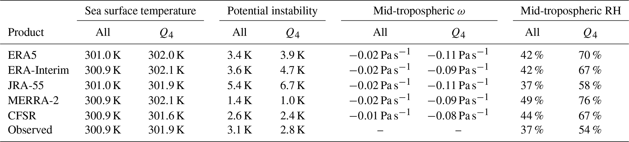
Figure 10b summarizes distributions of lower-tropospheric potential instability (defined as the difference in θe between 850 and 500 hPa; Eq. 2) for all tropical points and for points associated with Q4 of LWCRE. Values of potential instability in the tropics tend to be positive in all five reanalyses. However, this tendency is weaker for MERRA-2 and CFSR than for ERA5, ERA-Interim, or JRA-55, indicating systematic differences in the moist thermodynamic state of the tropical atmosphere (see also Table 3). Moreover, while ERA5, ERA-Interim, and JRA-55 indicate larger potential instabilities associated with Q4 of LWCRE than in the tropical mean; MERRA-2 and CFSR indicate the opposite. The latter is in better agreement with AIRS. For ERA-Interim, these differences may be linked to the convective closure (Appendix A2). The convection scheme in ERA-Interim specifies an adjustment timescale that, in practice, often exceeds the model time step (especially at coarser resolutions; Bechtold et al., 2008, their Fig. 1). Potential instability in convective locations (Q4) may thus be shifted toward larger positive values in ERA-Interim (Fig. 10b). The new closure (Bechtold et al., 2014) and finer model resolution used in ERA5 reduce the difference between the Q4 and tropical-mean values of potential instability by about 50 % (Table 3). The discrepancy between JRA-55 and the other reanalyses has a different origin. Figure 11a shows vertical profiles of MSE averaged over the upper and lower quartiles of daily gridded LWCRE within the inner tropics (10∘ S–10∘ N). A “kink” is evident in the vertical profile for JRA-55 between 900 and 850 hPa but not in any of the other profiles. This kink arises because the Q4 profile in JRA-55 has a warm bias at 850 hPa (+0.4 kJ kg−1 relative to ERA5; Fig. 11b, lower row) but a cool and dry bias at 900 hPa (total −1.0 kJ kg−1; not shown). The convective scheme in JRA-55 restricts cloud base to the model level at ∼900 hPa (JMA, 2013). Thermodynamic instabilities that develop at higher levels (such as the 850 hPa level used to compute potential instability) are thus difficult for the convection scheme to eliminate.
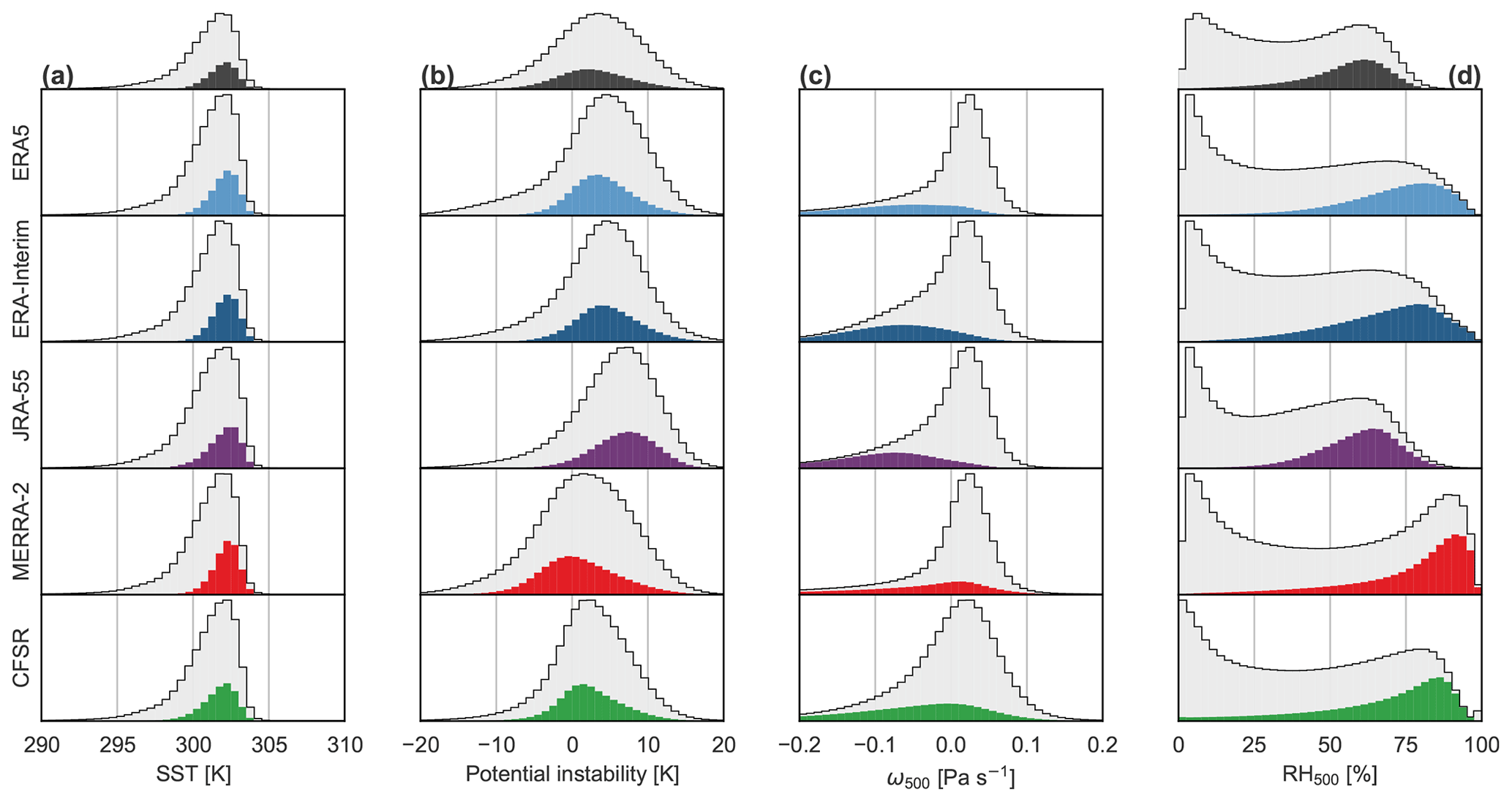
Figure 10Histograms of (a) sea surface temperature (SST), (b) potential instability (), (c) grid-scale vertical velocity in the middle troposphere (ω500), and (d) relative humidity in the middle troposphere (RH500). Data are based on daily-mean products at 1∘ × 1∘ resolution from (top to bottom) ERA5, ERA-Interim, JRA-55, MERRA-2, and CFSR during 2001–2010 in the inner tropics (10∘ S–10∘ N). Observational estimates are shown along the top axis where available, with data from CERES SYN1Deg (LWCRE), OISST v2 (SST), and AIRS (potential instability and RH500). Distributions that include AIRS data are for 2003–2010 rather than 2001–2010. Colour histograms show distributions for the top quartile of LWCRE in each data set (see Fig. 7). Mean values for each distribution are listed in Table 3.
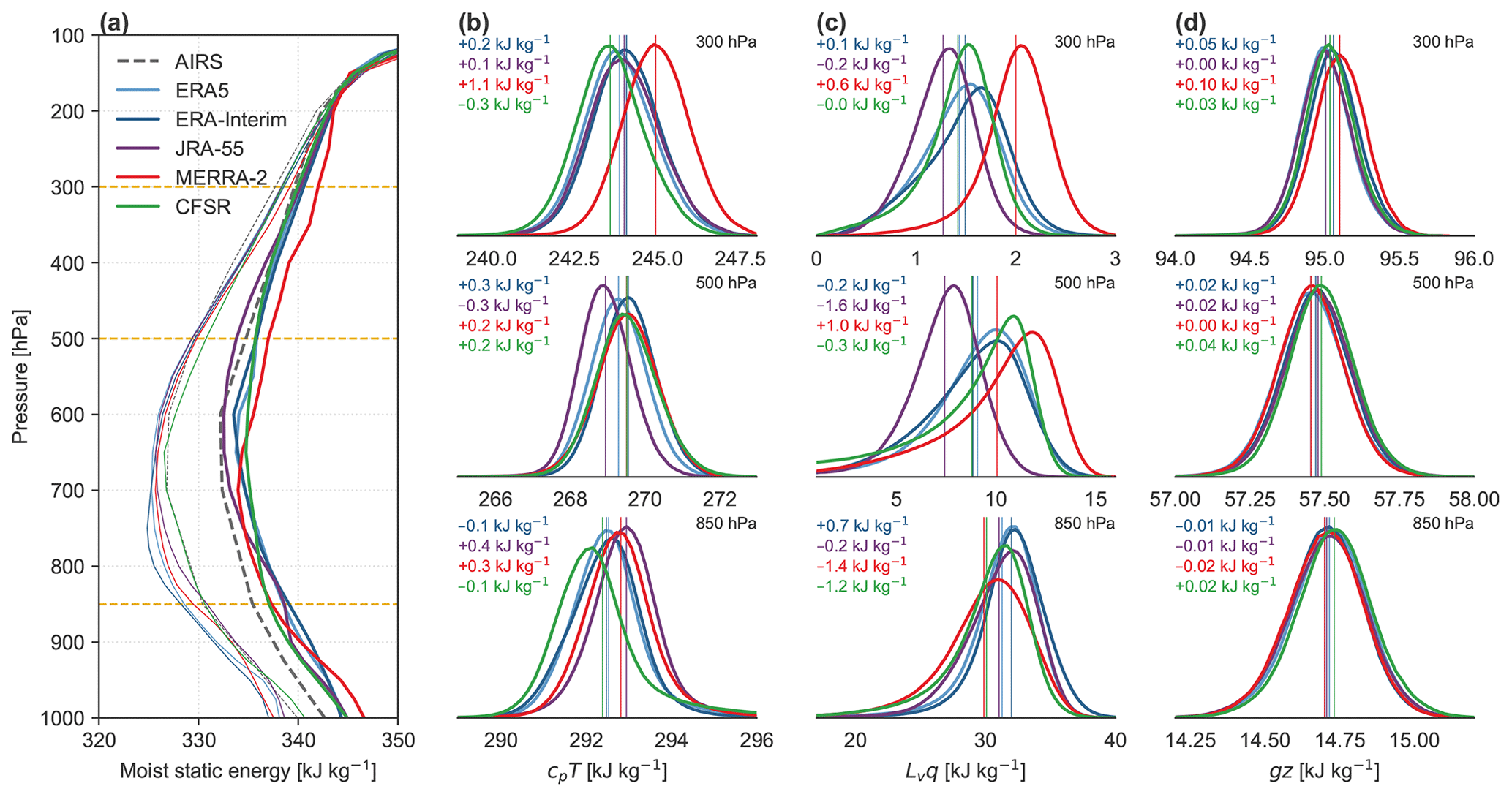
Figure 11(a) Composite vertical profiles of moist static energy (MSE) for ERA5 (cyan), ERA-Interim (blue), JRA-55 (purple), MERRA-2 (red), and CFSR (green) averaged for the upper (Q4; thick lines) and lower (Q1; thin lines) quartiles of daily-mean LWCRE during 2001–2010. Profiles calculated from AIRS observations (September 2002–December 2010; grey dashed lines) are conditioned on quartiles of daily-mean LWCRE from CERES SYN1Deg. At the right are distributions of the (b) temperature (cpT), (c) moisture (Lvq), and (d) geopotential (gz) components of MSE for Q4 from each reanalysis at the levels marked by yellow dashed lines in (a): 850 hPa (lower row), 500 hPa (centre row), and 300 hPa (upper row). Mean values are marked as vertical lines; biases in these mean values relative to the mean value from ERA5 are colour-coded at the upper left of each panel (each list from top: ERA-Interim, JRA-55, MERRA-2, and CFSR).
Decomposing differences in moist static energy into contributions from temperature, specific humidity, and geopotential (Fig. 11b–d), we find that the largest spreads result from differences in moisture content at both 850 and 500 hPa. At 850 hPa, latent energy (Lvq) based on CFSR and MERRA-2 is 1–2 kJ kg−1 less than that based on JRA-55, ERA5, or ERA-Interim (Fig. 11c, lower panel). Meanwhile, at 500 hPa, latent energy based on MERRA-2 is nearly 3 kJ kg−1 larger than that in JRA-55 and more than 1 kJ kg−1 larger than that in ERA5, ERA-Interim, or CFSR (Fig. 11c, middle panel). Biases in cpT are on the order of ±0.5 kJ kg−1 at both levels (Fig. 11b, lower two panels). For JRA-55 and MERRA-2, temperature biases compensate for humidity biases at 850 hPa but exacerbate the effects of humidity biases at 500 hPa. The relationship between potential instability and LWCRE in CFSR is most similar to that based on observations in terms of mean values, with AIRS estimates 0.4–0.5 K larger than those based on CFSR for both the tropics as a whole and the top quartile of LWCRE (Table 3). However, the distribution of potential instability based on AIRS is broader than that based on CFSR and in that sense is more reminiscent of the distributions based on MERRA-2 or ERA5 (Fig. 10b).
We briefly highlight two other features of the MSE profiles shown in Fig. 11a. First, lower-tropospheric values of MSE associated with Q4 are evidently larger in the reanalyses than in the AIRS observations. This may indicate that the reanalyses are systematically too moist or too warm in the lower troposphere but may also reflect systematic errors or sampling biases (e.g. cloud clearing) in the AIRS observations. Second, MERRA-2 shows much larger values of MSE in the upper troposphere of convective regions relative to other reanalyses. This bias results from both greater humidity (perhaps due to greater detrainment of cloud water and subsequent condensate evaporation; Fig. 4) and systematic warm biases (possibly linked to more intense cloud radiative heating at anvil level; Fig. 8). At 300 hPa, the excess Q4 MSE in MERRA-2 relative to ERA5 is on average 61 % attributable to differences in temperature (cpT; upper panel of Fig. 11b) and 33 % attributable to differences in moisture content (Lvq; Fig. 11c). The remainder (∼6 %) arises from differences in geopotential (Fig. 11d). This bias in upper-tropospheric MSE is systematic throughout the tropics (e.g. the Q1 profile in Fig. 11) but with smaller magnitudes and temperature biases contributing more outside of deep convective regions. Greater upper-tropospheric MSE in MERRA-2 implies stronger gross moist stability and specifically a stabilization of the upper troposphere that may suppress the average depth of convection. The lower, more extensive anvil deck in MERRA-2 contributes to both strong cloud top radiative cooling around 200 hPa (Fig. 8) and the inability of convective heating to compensate for this cooling. As noted previously for MERRA, this combination yields a physically implausible layer of time-mean zonal-mean diabatic descent centred near 200 hPa that extends across the entire tropics (Wright and Fueglistaler, 2013).
Figure 10c shows distributions of grid-scale vertical velocity (ω) in the middle troposphere (500 hPa). Distributions for the whole tropics are qualitatively similar across the five reanalyses, with peaks at small positive values (subsidence) and long tails toward large negative values (ascent). Larger values of LWCRE in ERA-Interim and JRA-55 are associated almost exclusively with grid-scale ascent in the middle troposphere. This relationship is less pronounced in MERRA-2 and CFSR, although the strongest mid-tropospheric ascent rates are associated with Q4 in all five reanalyses. These differences may be understood in terms of differences in the convective triggers (Appendix A2), which explicitly consider large-scale convergence in ERA-Interim and JRA-55 but not in MERRA-2 or CFSR. Dependence of the convective trigger on large-scale vertical velocity was eliminated from the ECMWF atmospheric model between the version used for ERA-Interim and that used for ERA5 (Bechtold et al., 2008). No observational benchmark is available for evaluating these distributions.
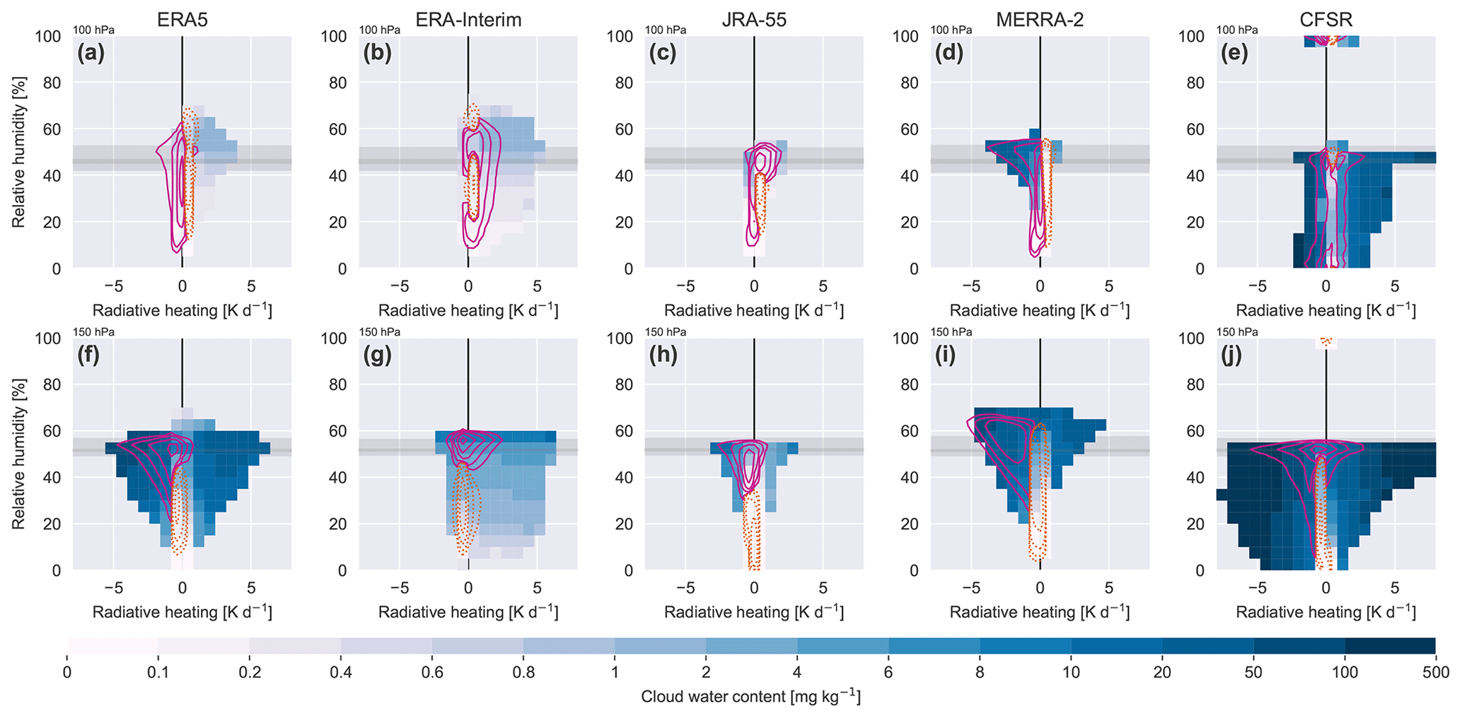
Figure 12Composite distributions of daily-mean CWC as a function of radiative heating rate and grid-scale relative humidity (RH) in (a, f) ERA5, (b, g) ERA-Interim, (c, h) JRA-55, (d, i) MERRA-2, and (e, j) CFSR on the 100 hPa (upper row; a–e) and 150 hPa (lower row; f–j) isobaric surfaces. RH is calculated with respect to liquid water. Grey shaded regions in each panel mark ranges of ice saturation ratios () at these levels, with light shading marking the minimum and maximum and dark shading marking the interquartile range. Solid pink contours mark paired values of radiative heating and RH that are more commonly associated with cloudy conditions (Q4 of the daily-mean LWCRE) than with clear-sky conditions (Q1 of LWCRE); dashed orange contours mark the opposite (values more commonly associated with Q1 than Q4). Composite mean CWCs are masked for bins containing fewer than 200 samples.
Distributions of mid-tropospheric RH (Fig. 10d; defined here with respect to liquid water) are bimodal in all five reanalyses, with peaks at both very small values (<10 %) and relatively large values (>50 %). The largest values of LWCRE tend to be associated with large values of mid-tropospheric relative humidity, although this relationship is tighter for MERRA-2 and CFSR than for ERA5, ERA-Interim, or JRA-55. The largest differences among the distributions are at the upper end of the range and can be at least partially explained by differences in the treatment of the liquid–ice transition (Appendix A; Fig. A1). As JRA-55 has the strictest transition from liquid to ice, mid-tropospheric RH with respect to liquid water is generally less than 75 %. ERA-Interim and ERA5 prescribe more gradual transitions from liquid to ice and thus produce larger relative humidities with respect to liquid water. Another potentially important parameter is the critical RH at which large-scale cloud formation (or evaporation of cloud water) is assumed to occur. This value is more than 90 % in MERRA-2 at 500 hPa as opposed to around 80 % in ERA5 and ERA-Interim, leading MERRA-2 to produce a larger frequency of very high relative humidities at this level. Tighter distributions of mid-tropospheric RH associated with the largest values of LWCRE (Fig. 10d) also suggest that deep convection may be more sensitive to mid-tropospheric entrainment of dry air in MERRA-2 and CFSR than in ERA5, ERA-Interim, or JRA-55. For MERRA-2 this is consistent with the application of a Tokioka-type entrainment condition (Bacmeister and Stephens, 2011): entrainment rates smaller than a randomly selected minimum (the Tokioka parameter) are disallowed. For small values of RH, entrainment is efficient in diluting the updraught so that plumes can only reach the upper troposphere when the entrainment rate is small. The Tokioka condition thus tightens the preference for deeper convection to occur in more humid environments. Entrainment rates are also relatively large in CFSR, which uses a base entrainment rate equal to the maximum rate in JRA-55 and about an order of magnitude larger than the base rate in ERA-Interim (Appendix A2). Among the reanalyses, the distribution of mid-tropospheric RH in JRA-55 is most consistent with that based on AIRS. However, as for lower-tropospheric MSE, caveats concerning sampling and cloud-clearance biases apply when interpreting the AIRS distribution.
5.2 Clouds in the TTL
Tropical high clouds in the reanalyses may also originate via the parameterized effects of grid- or subgrid-scale saturation. In the TTL, such in situ cloud formation is often associated with adiabatic cooling linked to wave activity or slow ascent (Massie et al., 2002; Schoeberl et al., 2019). Figure 12 summarizes relationships among CWC, radiative heating rates, and RH at isobaric levels near the base of the TTL (150 hPa) and near the tropopause (100 hPa). The TTL is located above the typical levels of convective detrainment (200–300 hPa; Fig. 4), with a lower boundary near the LZRH (140–150 hPa; Fig. 9a). Clouds in this layer are often associated with slow radiatively balanced ascent and occasionally with very deep convection that penetrates into the TTL (e.g. Fueglistaler et al., 2009). These two cloud populations may be distinguished by their CWCs (smaller for in situ cirrus; larger for convective anvil clouds) and associated radiative heating rates (weak radiative heating for slow ascent; strong cloud top cooling for most anvil clouds, possibly supplanted by strong warming for clouds reaching very high altitude). The essential radiative signature of cloud top cooling and cloud base warming can be seen by comparing the radiative heating profiles in Fig. 8a–e and the vertical locations of the anvil cloud layers in Fig. 4f. Radiative heating thus helps to distinguish different types of clouds in the lower part of the TTL: (1) in situ cirrus clouds, which are associated with weak positive heating rates balancing large-scale ascent (i.e. close to the “spine” of the plot); (2) deep convection that detrains near the base of the TTL, which is associated with large CWCs and negative radiative heating (the “left wing”); and (3) deep convection that detrains inside the TTL, which is associated with large CWCs and positive heating rates (the “right wing”). The latter two types are distinguished by both the depth and water content of the anvil cloud (Fig. 13), and the third type grows progressively rarer with increasing altitude. Compositing on RH in addition to radiative heating helps to highlight some differences and unrealistic features among the reanalyses, as discussed below.

Figure 13Composite mean profiles of cloud water content (CWC) from (a) ERA5, (b) ERA-Interim, (c) JRA-55, (d) MERRA-2, and (e) CFSR associated with different ranges of radiative heating rates at 150 hPa: negative rates less than −1 K d−1 (blue), neutral rates within ±1 K d−1 (grey), and positive rates greater than +1 K d−1 (red). Note different x axis ranges for CWC.
At 150 hPa, the distributions based on ERA5 (Fig. 12f) and MERRA-2 (Fig. 12i) show wings of large CWCs at large negative and large positive radiative heating rates bracketing a central axis in which radiative heating is weak and CWC depends mainly on RH. The largest values of LWCRE are associated with strong radiative cooling at 150 hPa (the left wing), while strong radiative heating (the right wing) is more often associated with Q2 or Q3 rather than Q4. This difference is consistent with composite mean profiles of CWC (Fig. 13): large negative heating rates at 150 hPa are associated with shallower anvils and larger CWCs, while large positive heating rates are associated with deeper anvils and smaller CWCs. The distribution based on JRA-55 (Fig. 12h) is similar to those based on ERA5 and MERRA-2 but with a smaller range of radiative heating rates, consistent with smaller anvil water contents (Fig. 4c). The distribution based on CFSR (Fig. 12j) also shows similarities but with additional variance in radiative heating linked to the occasional occurrence of extremely large daily-mean CWCs (up to 1408 mg kg−1) at this level. Approximately 1 % of daily-mean CWCs at 150 hPa in CFSR exceed 100 mg kg−1, far more than in any other reanalysis (maximum: 0.1 % in ERA5). The ERA-Interim distribution (Fig. 12g) is more distinctive, with CWC (and LWCRE) more tightly linked to RH and an asymmetry toward positive heating rates. ERA-Interim produces few instances of large negative heating rates, as clouds are associated with enhanced radiative heating at 150 hPa in this reanalysis (Fig. 8).
At 100 hPa, ERA5 and ERA-Interim (Fig. 12a and b) show similar distributions of composite mean CWC, as the largest values are associated with positive radiative heating and supersaturation with respect to ice. However, these two systems show different relationships with LWCRE. Whereas large values of LWCRE often correspond to positive heating rates at 100 hPa in ERA-Interim, the largest values of LWCRE typically correspond to negative heating rates at this level in ERA5. ERA5 and ERA-Interim are the only models considered here that explicitly consider supersaturation with respect to ice. Figure 12a and b indicates that, owing to different radiative signatures of deep convection within the TTL, in situ cirrus clouds form preferentially above strong convective regions in ERA-Interim but outside of these regions in ERA5. The distribution based on MERRA-2 is also bimodal (Fig. 12d), but in this reanalysis the most prominent mode is a leftward-facing wing with relatively large CWCs, negative radiative heating rates, and large LWCREs. This mode is consistent with cooling at the tops of anvil clouds near the tropical tropopause. The second mode features positive radiative heating rates and saturation with respect to ice and is thus consistent with expectations for thin high clouds near the tropopause (e.g. Fusina et al., 2007).
With the exception of ERA-Interim, the largest CWCs at 100 hPa are associated with very large water paths through the UTLS and large negative radiative heating at 100 hPa. The smallest CWCs at 100 hPa correspond to near-zero radiative heating. Mean CWCs associated with positive radiative heating ( K d−1) are significantly larger but still more than a factor of 10 smaller than those associated with strong negative radiative heating. Taking strong negative radiative heating ( K d−1) and large CWCs (>10 mg kg−1) at 100 hPa as a crude indicator of overshooting convection that reaches the tropopause, these events occur around 0.2 % of the time in MERRA-2 and 0.1 % of the time in CFSR and ERA5. These criteria are never met in JRA-55 or ERA-Interim. Conversely, taking large positive radiative heating ( K d−1) and above-average CWCs (>0.01 mg kg−1) as indicative of in situ cirrus in air rising through the TTL, this regime covers 35 % of the tropics in ERA-Interim; 24 % in JRA-55; and around 10 % in ERA5, MERRA-2, and CFSR.
The distribution based on CFSR at 100 hPa (Fig. 12e) indicates severe problems with humidity fields around the tropopause. Values of RH in CFSR at this level cluster around three values: zero (7 % of samples), saturation with respect to ice (6 %), and saturation with respect to liquid water (77 %). Values between zero and saturation with respect to ice account for the remaining 10 % of samples. Saturation with respect to liquid water occurs occasionally at 150 hPa in CFSR as well (Fig. 12j), although these instances differ from those at 100 hPa in that they are associated mainly with small values of LWCRE and negligible CWCs and only represent a small fraction of samples (1.5 %). Humidity fields in the stratosphere are unrealistically small in CFSR (Davis et al., 2017); Fig. 12 shows that unrealistic behaviour often extends downward into the TTL. In Appendix B, we show that the situation is much improved in CFSv2.
Although MERRA-2 contains no explicit representation of ice supersaturation, RH in this reanalysis exceeds saturation with respect to ice in around 33 % of gridded daily means at 150 hPa and 20 % of gridded daily means at 100 hPa. This decrease with height differs from the parameterized behaviour in ERA-Interim and ERA5, in which daily-mean supersaturation frequencies increase from 15 %–25 % at 150 hPa to 30 %–40 % at 100 hPa. The occurrence of ice supersaturation in MERRA-2 can result from the partitioning of liquid and ice and subsequent gradual relaxation of liquid condensate to ice as implemented in the model's prognostic cloud scheme (Appendix A1), but it is surprising that it remains so prevalent in the TTL. This feature may result from temporal truncation: the model limits the water vapour content at grid-scale saturation; the temperature is then modified by some other process; and output is written without further adjustment to the water vapour field. All of the supersaturated points in MERRA-2 have non-zero CWCs, and CWC tends to increase with increasing supersaturation (r=0.24). Liquid water is present in trace amounts for almost all supersaturated points at 150 hPa (93 %) and a substantial fraction of supersaturated points at 100 hPa (31 %). This persistence of positive liquid water contents at very low temperatures will be addressed in a forthcoming version of the GEOS-5 model.
Figure 14 shows deseasonalized monthly anomalies for HCC, all-sky OLR, clear-sky OLR, and LWCRE in the inner tropics (10∘ S–10∘ N) based on the five reanalyses and CERES-based data sets (CERES SYN1Deg for HCC; CERES EBAF for OLR and LWCRE). Anomalies are calculated relative to the mean annual cycle over all full years in the CERES overlap period (2001–2014). Most of the reanalyses produce temporary increases in high-cloud fraction and LWCRE (and corresponding decreases in OLR) around the major El Niño events of 1982–1983 and 1997–1998, although the timing, amplitude, and duration of these excursions varies. However, the most pronounced variations appear to be artificial. Most notably, the tropical-mean HCC in CFSR jumped suddenly by more than 0.1 between the end of 2009, when CFSR was initially planned to end, and the beginning of 2010. Tropical-mean HCC then jumped again at the beginning of 2011 with the transition to CFSv2 to a value very close to that in MERRA-2 (not shown). The bridge year 2010 is not well documented but has been shown to feature discontinuities in other variables as well (e.g. stratospheric water vapour; Davis et al., 2017). Abrupt changes in the CFSR time series are not limited solely to the CFSR–CFSv2 transition, with transient reductions in tropical-mean HCC after every production stream transition in the initial 1979–2009 run (1 January 1987, 1990, and 1995; 1 April 1999 and 2005; Saha et al., 2010; Fujiwara et al., 2017). However, whereas these stream-related discontinuities are also seen in OLR and LWCRE (as is the transition at the beginning of 2010), neither OLR nor LWCRE shows sudden changes following the transition to CFSv2 in January 2011. Despite suggestions that CFSv2 can serve as an extension of CFSR, researchers should be cautious in adopting this approach for studies that span the 2010 bridge year or the 2011 transition to CFSv2. Further discussion of the CFSR–CFSv2 transition is provided in Appendix B.
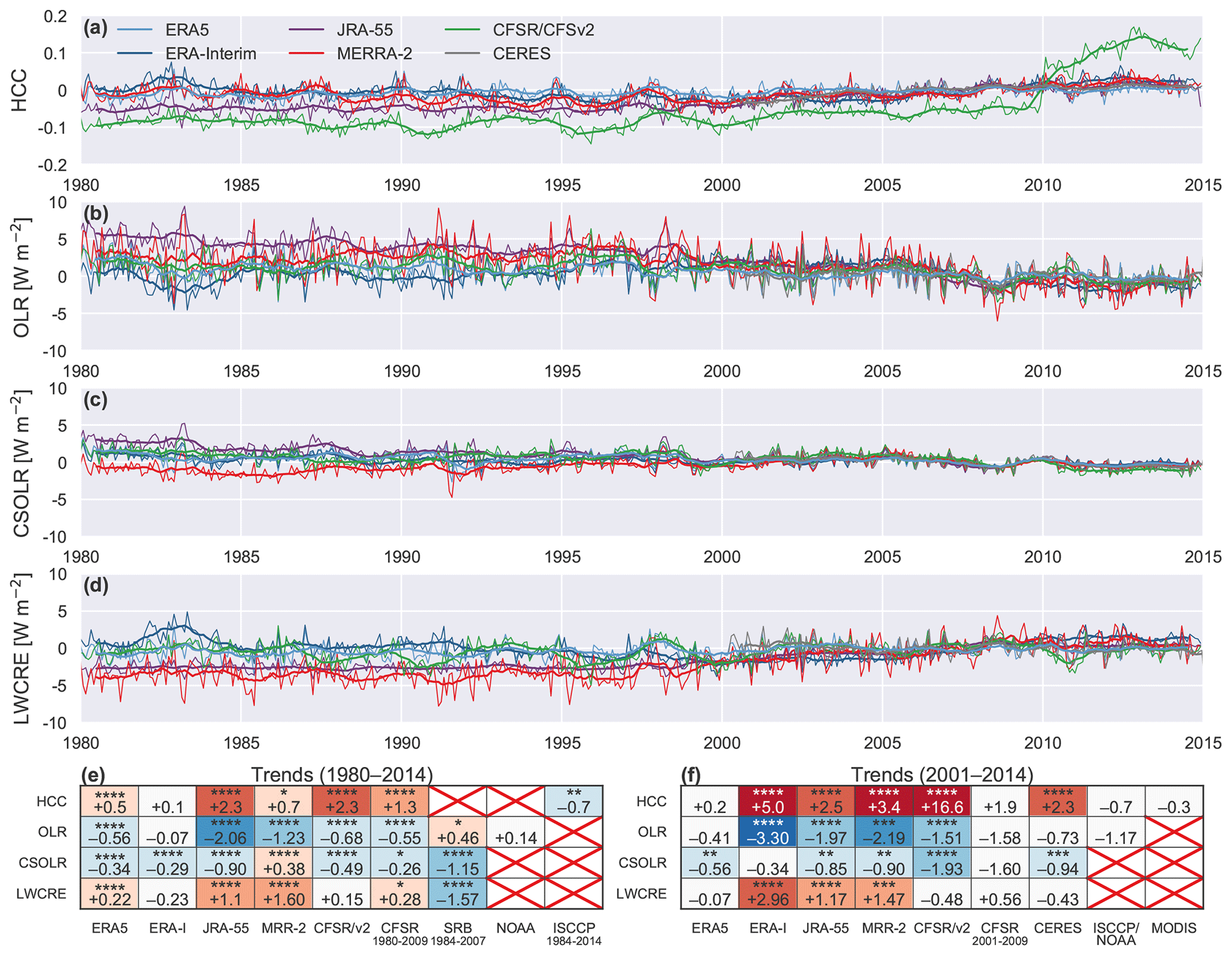
Figure 14Time series of deseasonalized anomalies in monthly-mean (a) HCC, (b) all-sky OLR, (c) clear-sky OLR (CSOLR), and (d) LWCRE averaged over the inner tropics (10∘ S–10∘ N) for 1980–2014 based on ERA5 (cyan), ERA-Interim (blue), JRA-55 (purple), MERRA-2 (red), and CFSR/CFSv2 (green). Observational analyses from CERES SYN1Deg (a; March 2000–December 2014) and CERES EBAF (b–d; March 2000–December 2014) are shown for context. Anomalies are calculated relative to the mean annual cycle during 2001–2014. Thick lines show time series after applying a 12-month uniformly weighted rolling mean. Trends are listed for annual-mean anomalies during the (e) 1980–2014 and (f) 2001–2014 periods in percentage points per decade for HCC and units of watts per square metre per decade for OLR, clear-sky OLR, and LWCRE (in which ERA-Interim is abbreviated ERA-I and CFSR/CFSv2 is abbreviated CFSR/v2). Stars indicate statistical significance at the 90 % (*), 95 % (), 99 % (), and 99.5 % () confidence levels. Light-grey shading indicates that the 90 % confidence interval of the Theil–Sen slope (Sen, 1968) contains zero. Blue colours mark negative trends and red colours positive trends, with darker shades signifying larger trend magnitudes (0 to 1, 1 to 2, 2 to 3, and greater than 3).
In addition to the production stream transitions in CFSR/CFSv2, several of the anomaly time series show long-term drifts. To assess the consistency of these long-term changes across data sets, we evaluate trends over the 1980–2014 and 2001–2014 periods (Fig. 14d and e). Note that even where trends are statistically significant, their signs and magnitudes are subject to uncertainties associated with data processing and changes in the observing system over time. These caveats apply not only to reanalyses but also to observationally based analyses (like the ISCCP and CERES cloud products; e.g. Dai et al., 2006) and derived products that depend on these analyses (like the SRB and CERES clear-sky radiation products; e.g. Trenberth et al., 2009). Trends are shown here for intercomparison purposes, without assessment of their realism or reliability.
Over the full record, JRA-55 shows the most obvious and temporally consistent increase in HCC, along with corresponding changes in OLR (towards smaller values) and LWCRE (towards larger values). These changes bring JRA-55 closer to the other reanalyses, although absolute biases in tropical-mean OLR relative to ERA-Interim and CFSR/CFSv2 remain on the order of 10 W m−2 over 2010–2014 (as opposed to ∼15 W m−2 in the early 1980s). Most of the other reanalyses show qualitatively similar trends in HCC (increasing), OLR (decreasing), and LWCRE (increasing) over 1980–2014 but with magnitudes smaller than those based on JRA-55. Decreasing trends in clear-sky OLR are qualitatively robust, except for the 1980–2014 trend in MERRA-2. Decreasing trends in clear-sky OLR suggest that increases in atmospheric greenhouse gas absorption outpaced increases in the effective emission temperature in the tropics over this period, which may be explained by the so-called “hiatus” in surface warming during the early 2000s (Song et al., 2016). Prescribed greenhouse gas concentrations increased throughout this period (Fujiwara et al., 2017, their Fig. 4), even as observed surface temperatures cooled or stayed roughly constant through much of the tropics (e.g. Kosaka and Xie, 2013). Although these trends should be interpreted with care, their consistency with expectations may be a promising sign for the use of broadband OLR fluxes in climate monitoring, given the potential for compensating effects to damp signals of climate change in these fields (e.g. Huang and Ramaswamy, 2009).
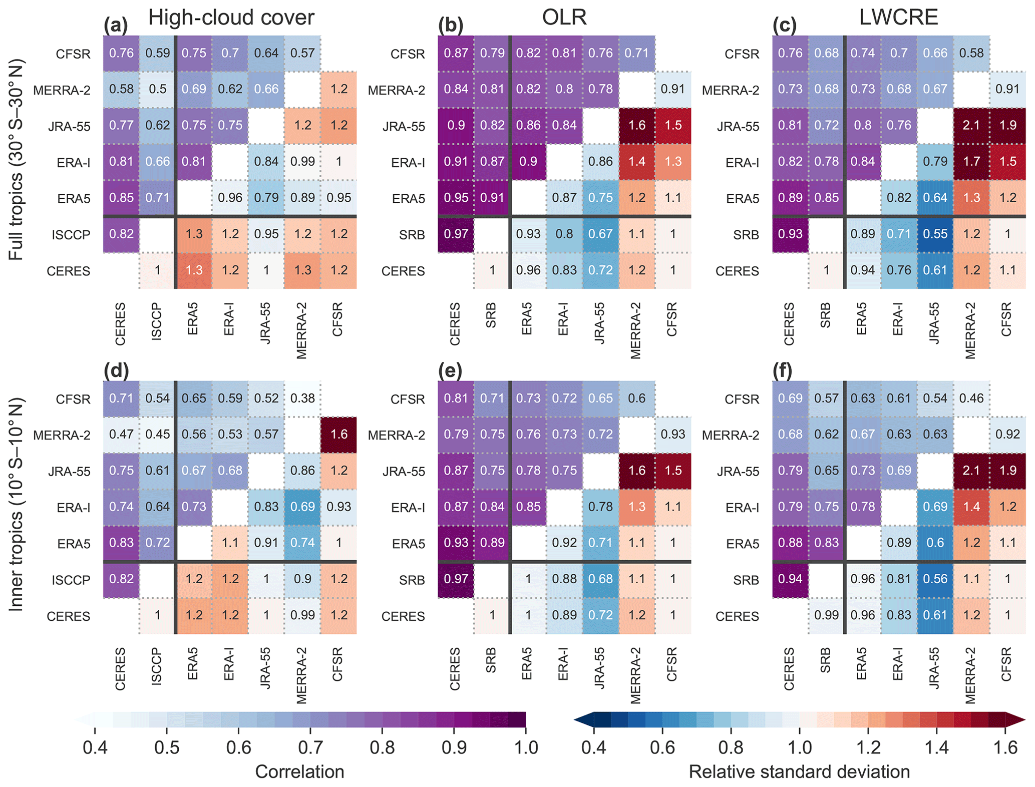
Figure 15Metrics measuring agreement in monthly anomalies of (a, d) HCC, (b, e) OLR, and (c, f) LWCRE among the reanalyses and observational data sets examined in this paper (in which ERA-Interim is abbreviated ERA-I). The upper-left triangle in each panel shows correlation coefficients between each pair of products, while the lower-right triangle shows the standard deviation in the product marked on the horizontal axis relative to that in the product marked on the vertical axis. Both metrics are evaluated first for individual grid cells in the 2.5∘ common grid (see e.g. Fig. 1) and then averaged. The upper row (a–c) shows results for the entire tropics (30∘ S–30∘ N), while the lower row (d–f) shows results for the inner tropics only (10∘ S–10∘ N). Solid black lines separate evaluations relative to the observational benchmarks based on CERES, ISCCP, and NASA/GEWEX SRB from those based on intercomparison of reanalysis products.
Most of the reanalyses also suggest decreasing trends in all-sky OLR over this period, although the signs (over 1980–2014) and magnitudes (over 2001–2014) of these trends are not supported by observations. Associated declines in upwelling LW radiation at the tropopause may help to explain long-term decreases in tropical cold-point temperatures based on JRA-55, MERRA-2, and CFSR (Tegtmeier et al., 2020). Decreasing trends in all-sky OLR seem at first glance to contradict the fixed anvil temperature hypothesis of Hartmann and Larson (2002). However, increasing trends in HCC are qualitatively consistent with decreases in all-sky OLR above and beyond those in clear-sky OLR; reductions in all-sky OLR therefore do not necessarily imply reductions in anvil cloud emission temperatures. Indeed, with the exception of CFSR/CFSv2 (affected by discontinuities around the CFSR–CFSv2 transition as discussed in Appendix B) and ERA5 (for which trends are small), relatively large decreasing trends in all-sky OLR among reanalyses reflect relatively large increases in LWCRE, which are linked in turn to increases in HCC. The increases in LWCRE and HCC implied by reanalyses are generally not supported by the observationally based time series; however, discrepancies in HCC trends among CERES (positive), ISCCP (negative), and MODIS (no significant trend) reveal endemic uncertainty regarding whether and in what direction this variable changed. Long-term trends over 1980–2014 are small in both ERA5 and ERA-Interim. This picture changes considerably in the later part of the record, for which trends in ERA5 remain small but trends in ERA-Interim are among the largest across all data sets. For ERA-Interim, weak long-term trends thus reflect relatively large excursions in these variables in the early 1980s acting to offset relatively large changes in the same direction after the turn of the century. These early-1980s excursions have also been reported for TTL temperatures based on ERA-Interim (Tegtmeier et al., 2020).
Figure 15 summarizes paired correlations and normalized standard deviations among the five reanalyses and available observation-based benchmarks. Monthly anomalies and evaluation metrics are calculated for the longest overlapping period common to both data sets (CERES: 2001–2014; ISCCP and SRB: 1984–2007; CFSR: 1980–2009; all other reanalyses: 1980–2014). For CFSR we truncate the time series after 2009 to avoid the 2010 bridge year and the CFSR–CFSv2 transition. Extending the time series through 2014 reduces the correlations and increases the normalized standard deviations. Two sets of summary results are provided, one for the tropics as a whole (30∘ S–30∘ N; Fig. 15a–c) and one for the inner tropics (10∘ S–10∘ N; Fig. 15d–f). Correlations and standard deviations are calculated first for data on a common 2.5∘ × 2.5∘ latitude–longitude grid and then averaged for the corresponding region.
Among the reanalyses, monthly anomalies based on ERA5 consistently show the highest correlations against observational benchmarks for all metrics (HCC, OLR, and LWCRE), regions (full tropics and inner tropics), and analysis periods (1984–2007 for ISCCP and SRB and 2001–2014 for CERES). By contrast, MERRA-2 shows relatively poor correlations for HCC, especially in the inner tropics. Correlations for HCC relative to CERES are larger than those relative to ISCCP for all five reanalyses. Although this difference is also found for CERES versus SRB with respect to variability in OLR and LWCRE, the difference is less pronounced in these cases. Paired correlations for OLR and LWCRE almost all exceed 0.7, with only correlations against CFSR (complicated by the issues around production stream transitions) falling below 0.6.
Most of the reanalyses (except for JRA-55 in both regions and MERRA-2 in the inner tropics) show stronger variability in HCC than indicated by CERES SYN1Deg or ISCCP D2. However, this may reflect shortcomings in the observational analyses, such as sampling biases or limited sensitivity to optically thin clouds. The smaller standard deviation in HCC in JRA-55 is likewise consistent with JRA-55 tending to underestimate HCC relative to the other reanalyses (Fig. 1e). Conversely, the results for MERRA-2, where variability is stronger than observed when averaged over the full tropics and weaker than observed when averaged over the inner tropics, may be associated with MERRA-2 producing persistently large cloud fractions outside of the core convective regions (Fig. 1g). Results for variations in OLR and LWCRE are fairly robust, with JRA-55 consistently underestimating variability and MERRA-2 consistently overestimating variability relative to all other data sets. ERA-Interim also tends to underestimate variations in OLR and LWCRE relative to CERES or SRB. Standard deviations based on ERA5 and CFSR are similar to those observed.
We have presented and evaluated differences in tropical high clouds and their radiative impacts in five recent reanalyses: ERA5, ERA-Interim, JRA-55, MERRA-2, and CFSR. As a general rule, JRA-55 has less cloud water and smaller high-cloud fractions than other reanalyses in the tropical upper troposphere (Figs. 1, 3, and 4). MERRA-2 represents the opposite bookend, with more cloud water and larger high-cloud fractions. Accordingly, JRA-55 significantly overestimates OLR and underestimates the top-of-atmosphere LWCRE in the tropics relative to observations and other reanalyses, while MERRA-2 produces smaller values of OLR and larger values of LWCRE, in better agreement with observations (Figs. 5–7). Tropical-mean values from ERA-Interim and CFSR are similar to each other (and to the multi-reanalysis means) despite substantially different bias distributions. Relative to these two reanalyses, ERA5 produces slightly larger cloud fractions and smaller values of OLR.
Systematic differences in CWC translate into differences in radiative heating rates within the tropical upper troposphere and lower stratosphere (Fig. 8), with the largest CWCs (MERRA-2) corresponding to extensive disruption of the radiative heating profile and the smallest CWCs (ERA-Interim and JRA-55) corresponding to relatively weak effects. On one extreme, large CWCs in MERRA-2 result in a physically unreasonable time-mean zonal-mean layer of diabatic cooling in the tropics around 200 hPa (e.g. Tao et al., 2019, their Fig. D1). A similar layer in MERRA has been shown to cause problems with transport simulations in the TTL (e.g. Schoeberl et al., 2012). On the other extreme, the vertical distribution of CWC in ERA-Interim lacks the distinctive anvil layer found in observations and other reanalyses (Fig. 4). As a result, only ERA-Interim among these five reanalyses indicates that cloud effects typically shift the LZRH toward lower altitudes (Fig. 9a). All other reanalyses indicate upward shifts, with the largest shift in MERRA-2. It is worth noting that an upward shift contradicts results based on applying radiative transfer models to observed cloud distributions, which indicate that cloud effects lower the LZRH (Corti et al., 2005; Fueglistaler and Fu, 2006; Yang et al., 2010). This disagreement appears to arise from a combination of the reanalyses locating the peak positive short-wave effect at lower altitudes and overestimating the negative long-wave effect (Fig. 8; cf. Yang et al., 2010, their Fig. 10). The former suggests that the reanalyses may systematically underestimate the depth of convective anvil clouds, although this is not immediately evident in Figs. 3 or 4. For the latter, systematic underrepresentation of thin cirrus clouds and their radiative effects within the TTL seems a likely explanation (Corti et al., 2005; Yang et al., 2010), especially as we represent cloud effects here in terms of the relative magnitude of LWCRE.
Heating rates in the lower stratosphere are also impacted by differences in high clouds (Fig. 9b; Norton, 2001; Fueglistaler and Fu, 2006; Tao et al., 2019). Large CWCs and a strong LWCRE, as in MERRA-2, correspond to weaker convergence of LW radiation (and hence weaker diabatic ascent) in the tropical lower stratosphere. Conversely, small CWCs and a weak LWCRE, as in JRA-55 or ERA-Interim, correspond to stronger diabatic ascent in this region. At the nominal TOA, most of the reanalyses show substantial compensation between LWCRE and SWCRE associated with thick high clouds, as the largest LWCREs are also associated with relatively large opposing SWCREs (Figs. 6 and 7). Exceptions are JRA-55, in which a weak LWCRE and a strong SWCRE result in a negative bias in the total CRE, and CFSR, in which a moderate LWCRE and a weak SWCRE result in a positive bias in the total CRE in the inner tropics. The latter is compensated by negative biases in the subtropics (Fig. 6), yielding a net CRE in good agreement with CERES over the entire 30∘ S–30∘ N band but with much sharper horizontal gradients. As differences in clear-sky fluxes are comparatively small, these differences in cloud effects translate to a net loss of energy by the tropical atmosphere in JRA-55 and a net gain of energy by the tropical atmosphere in CFSR relative to other reanalyses. These radiative biases may in turn contribute to differences in other processes, such as horizontal energy advection, convective activity, or adjustments due to data assimilation. Many of the differences in high clouds and their radiative impacts can be traced back to assumptions and simplifications applied in the model convection schemes or in special treatments of detrained condensate in the prognostic cloud scheme. However, the differences also involve feedbacks between parameterized cloud fields and the tropical environment that are not fully mitigated by observational data assimilation.
The reanalyses demonstrate a range of cloud behaviours near the tropical tropopause (Figs. 12 and 13). Further evaluation will be needed given the current lack of observational constraints, but values in CFSR are noticeably unrealistic (Fig. 12e and j). Water vapour and cloud fields from CFSR should be avoided at these levels, although these issues appear to be improved in CFSv2 (Fig. B1). We have also reported evident discontinuities at production stream transitions in CFSR (Fig. 14), indicating that this data set should be used with caution, especially in analyses that span the 2010 bridge year and/or the 2011 transition to CFSv2 (see also Appendix B). Taking all factors into account (an absence of major drifts or jumps, consistently high correlations, and standard deviations quite close to those found in observationally based analyses), ERA5 appears to provide a better representation of temporal variability in HCC, OLR, and LWCRE within the tropics than other recent reanalyses. However, it is important to note that the current version of ERA5 contains known discontinuities in some variables in the early 2000s (e.g. temperature biases around and above the tropopause; Hersbach et al., 2018). ERA5.1, a rerun covering the problematic period, has recently been released to address this issue.
We have highlighted several notable differences between ERA-Interim and ERA5 that may be of interest to users familiar with ERA-Interim. First, ERA5 produces more extensive cloud cover than ERA-Interim over continental convective regions in the tropics (Fig. 1c and d). This difference has previously been reported to reduce brightness temperature biases in these regions (Bechtold et al., 2014). Second, the maximum cloud fraction in the tropical upper troposphere is shifted to lower altitudes in ERA5 relative to ERA-Interim (Fig. 3a and b). Comparison with observations does not clearly demonstrate which of these is more realistic (Fig. 3f). Third, a pronounced anvil maximum in CWC is present in the tropical upper troposphere in ERA5 but not in ERA-Interim (Fig. 4a and b). The distribution in ERA5 is more consistent with CloudSat observations but still shows substantial discrepancies (Fig. 4f). Fourth, as a consequence of the increased CWC in the upper troposphere, the positive bias in OLR and negative bias in LWCRE in ERA-Interim are both reduced in ERA5 (Fig. 5). Distributions of LWCRE, SWCRE, and total CRE based on ERA5 are more consistent with those inferred from CERES data (Fig. 7). However, in both ERA5 and ERA-Interim, low biases in LWCRE relative to CERES EBAF are twice as large in absolute magnitude as high biases in OLR because clear-sky OLR is underestimated, while all-sky OLR is overestimated. This may indicate issues with composition, emissivity, or other aspects of the LW radiation scheme in addition to clouds. We find the same behaviour in CFSR/CFSv2, which uses the same base model for LW radiative transfer as ERA5 and ERA-Interim (Appendix A3). Finally, cloud effects on radiative heating rates in the tropical upper troposphere, tropopause layer, and lower stratosphere are very different between ERA5 and ERA-Interim (Fig. 8). Results for ERA5 are more in line with those found in other reanalyses (as noted above for the LZRH; Fig. 9) but should be further evaluated (such as the CloudSat fluxes and heating rates product; L'Ecuyer et al., 2008).
Much of the information on the origins and impacts of biases in high clouds in this paper derives from relationships between cloud cover and other variables, including radiative exchange and the moist thermodynamic environment. Such comparisons not only help to reveal issues in the cloud parameterizations but also highlight where and in what ways such issues may affect reanalysis variables more tightly constrained by the data assimilation, such as temperatures, winds, and humidities. The vertical profile of moist static energy (Fig. 11) is an instructive example. MSE is calculated solely using variables targeted by data assimilation. However, our results reveal important differences in the vertical profile of MSE, especially in convective regions. Nor are these differences attributable solely to discrepancies in the water vapour fields, as illustrated by the stabilizing effects of upper-tropospheric warm biases in MERRA-2. Biases in upper-tropospheric temperatures imply differences in the vertical location and spatiotemporal variability of isentropic surfaces as well. Such differences may impact the results of reanalysis-driven transport model simulations, regardless of whether those studies assume isentropic, diabatic, or kinematic representations of vertical motion. It is worth reiterating that we use the “assimilated” (ASM) products from MERRA-2, which derive from the IAU corrector forecast, as opposed to the “analysed” (ANA) outputs, which derive from the 3D-FGAT analysis directly. The latter are expected to provide a closer match with the assimilated observations. However, in the case of MSE the ANA and ASM products are still in closer agreement with each other (figure not shown) than with AIRS or other reanalyses: both MERRA-2 products show large positive biases in the upper troposphere over convective regions. We have focused on the ASM products in this intercomparison both because these variables are self-consistent with MERRA-2 cloud and radiation products and because NASA GMAO (Global Modeling and Assimilation Office) recommends the use of ASM products over ANA products in transport model simulations.
Several observationally based data sets are used to establish context for the cloud fields. Such observationally based analyses are limited by perspective, especially when clouds occur in multiple overlapping layers, and the information that goes into them is neither homogeneous in space nor continuous in time. Both issues can be addressed to some extent, the former through the use of active remote sensing techniques such as lidar and radar (Stephens and Kummerow, 2007) and the latter through systematic analyses of imagery collected by the global network of geostationary satellites (Rossow and Schiffer, 1999), but no current observational platform addresses both simultaneously. Moreover, discrepancies among observationally based estimates arising from differences in measurement capabilities and techniques remain large (e.g. Pincus et al., 2012; Stubenrauch et al., 2013) and appear to be at least comparable in magnitude to discrepancies among recent reanalyses (Fig. 3). Observational constraints on reanalysis (and other model-based) cloud fields therefore remain more qualitative than quantitative. Observation simulators can help, not least by enabling new sets of sensitivity tests (e.g. Stengel et al., 2018), but are still limited to the cloud populations that can be effectively observed by the observational platforms being emulated.
We have largely neglected cloud top height and cloud top temperature in this intercomparison. The rationale for this omission is that the reanalyses do not typically provide these metrics directly, and they must be inferred by other means. However, systematic biases in cloud top heights or temperatures may have implications for the magnitude and distribution of cloud radiative effects. Such biases may also influence the spatiotemporal distribution of convective source regions of air entering the stratosphere as inferred from transport model simulations. A systematic intercomparison of cloud top heights and temperatures may be useful for revealing further deficiencies or idiosyncrasies of the convective parameterizations used in the reanalysis models. Further investigation along these lines may also consider how these features can imprint upon more widely used reanalysis products and model simulations that use reanalysis fields to drive atmospheric transport.
In this appendix, we briefly document selected aspects of the cloud, convection, and radiation parameterizations in the reanalysis atmospheric models. Additional information on the models, data assimilation schemes, and other elements of the reanalysis systems has been provided by Fujiwara et al. (2017) and in Chapter 2 of the forthcoming SPARC Reanalysis Intercomparison Project report (Wright et al., 2020, review version available at https://jonathonwright.github.io/S-RIPChapter2E.pdf, last access: 15 July 2020).
A1 Prognostic cloud parameterizations
All reanalyses examined in this paper use prognostic parameterizations of large-scale clouds that consider two sources of high clouds: detrainment from deep convection and in situ condensation associated with large-scale vertical motion or diabatic cooling. The evolution of high clouds in ERA-Interim is governed by the scheme outlined by Tiedtke (1993), in which a pair of equations are used to simultaneously track cloud water mass and cloud fraction accounting for transport, convective, and large-scale source terms, as well as losses due to evaporation and precipitation. The scheme does not distinguish between liquid water and ice; rather, the ice phase fraction is diagnosed as a quadratic function of temperature between 0 ∘C (entirely liquid) and −23 ∘C (entirely ice) at each time step (Fig. A1). The model also includes a parameterization to represent supersaturation with respect to ice at temperatures below −23 ∘C. ERA5 uses an updated version of the same scheme. One of the most important changes is that both liquid and ice condensate are treated prognostically in ERA5, eliminating diagnostic partitioning between the two phases. The resulting behaviour cannot be easily summarized in Fig. A1, but a comparison between the approach used in ERA5 and that used in ERA-Interim has been provided by Forbes et al. (2011, their Fig. 3). Clouds are assumed to be exclusively ice at temperatures below −40 ∘C. Parameterized supersaturation with respect to ice applies at all temperatures below the freezing point in ERA5, rather than only at temperatures below −23 ∘C as in ERA-Interim. JRA-55 uses a version of the approach suggested by Sommeria and Deardorff (1977) and modified by Smith (1990) to represent large-scale clouds at high altitudes. Cloud fraction depends on joint probability density functions (PDFs) of total water content and liquid water temperature (, with qc as the cloud water content), assuming uniform distributions of subgrid fluctuations in both variables. Note that this formulation differs from the large-scale condensation scheme used to represent the evolution of marine stratocumulus, which follows Kawai and Inoue (2006). Partitioning between the ice and liquid phases is determined as a linear function of temperature between 0 and −15 ∘C (Fig. A1). Like JRA-55, MERRA-2 also uses a two-moment PDF-based approach to represent cloud cover and cloud water content but with the total water PDF constrained as suggested by Molod (2012). Condensate formed in anvil clouds and condensate formed via large-scale saturation are tracked separately in the prognostic cloud scheme, with “anvil condensate” gradually converted to “large-scale condensate” (Bacmeister et al., 2006). New condensate is partitioned among the liquid and ice phases as a linear function of temperature between 0 and −20 ∘C (Fig. A1), with liquid condensate gradually converted to ice in the prognostic scheme when temperatures are less than 0 ∘C. The approach used in MERRA is similar to that used in MERRA-2 but with a quartic function governing the partitioning of new condensate into liquid and ice (Fig. A1) and without the constraints on total water proposed by Molod (2012). In CFSR and CFSv2, cloud water content is parameterized using the formulation of Zhao and Carr (1997). Cloud fraction is then diagnosed following Xu and Randall (1996). Cloud water content is the primary determinant of cloud fraction, with RH being a secondary contributor. The cloud scheme does not explicitly distinguish between liquid and ice. Condensate is assumed to be liquid for temperatures greater than 0 ∘C and ice for temperatures less than −15 ∘C (Fig. A1). At temperatures between these bounds, condensate is assumed to be liquid unless ice crystals already exist at or above the grid cell.
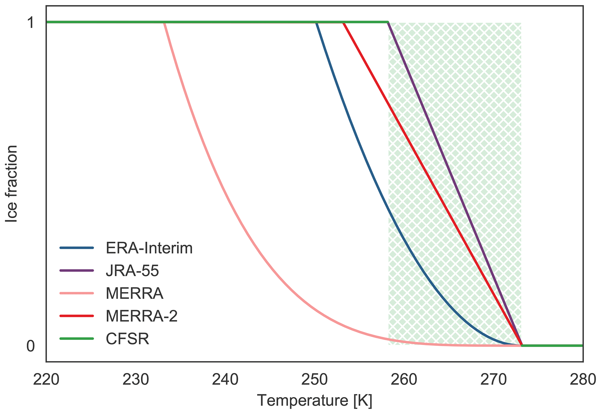
Figure A1Fraction of new condensate in the ice phase as a function of temperature for ERA-Interim (blue), JRA-55 (purple), MERRA (light red), MERRA-2 (dark red), and CFSR (green). The green shaded region with hatching marks the range of temperatures for which new condensate in CFSR is assigned to the ice phase if ice already exists at or above the grid cell in question and is assigned to the liquid phase otherwise.
All six reanalyses allow for evaporation and sublimation of condensed water and ice, along with losses of condensate due to autoconversion, accretion, and sedimentation. As with the parameterized formation of clouds, parameterizations of these loss processes differ amongst the reanalyses. For example, while all six reanalyses allow for condensate loss to vapour when grid-scale RH falls below a critical threshold, only ERA5, ERA-Interim, MERRA, and MERRA-2 explicitly include representations of “cloud munching” (evaporative loss due to turbulent mixing with clear air near the edges of the cloud; e.g. Del Genio et al., 1996). These parameterizations depend on the saturation specific humidity or vapour pressure and therefore have less effect for clouds at high altitudes (where temperatures are low) than for clouds at low altitudes. The cloud-munching parameterizations in MERRA and MERRA-2 apply only to anvil-type condensate detrained from deep convection. Implementations of the critical threshold for cloud evaporation are also influential. For example, lowering the critical threshold from saturation to the critical RH used for cloud formation contributes to increases in cloud residence times and re-evaporation of ice particles between MERRA and MERRA-2 (Molod et al., 2012).
A2 Parameterizations of deep convection
All six reanalyses apply mass-flux representations of deep convection (e.g. Arakawa and Schubert, 1974; Tiedtke, 1989) but with substantially different treatments (Table A1). Mass-flux convective parameterizations represent the statistical effects of convection in a given grid cell via one or more updraught and downdraught plumes. Both updraught and downdraught plumes are then coupled to the background environment via entrainment and detrainment, diabatic heating, and the vertical transport of tracers and momentum. Differences in the convective parameterizations used by the reanalysis systems include the trigger function, the principal closure, whether and to what extent momentum and tracer transport are included, constraints on the properties of the individual plumes (e.g. entrainment, detrainment, cloud base, and cloud top), and assumptions governing the production and partitioning of rainfall and cloud condensate.
ERA-Interim uses the scheme proposed by Tiedtke (1989), with a single pair of plumes representing updraughts and downdraughts. Deep convection is triggered when the updraught vertical velocity diagnosed at the lifting condensation level (LCL) is positive and the estimated cloud depth exceeds 200 hPa (Bechtold et al., 2006). Convection can be triggered from any level in the lowest 350 hPa of the atmosphere. Active convection consumes convective available potential energy (CAPE) over a specified timescale of 60 min. ERA5 uses the same core convection scheme as ERA-Interim (Table A1) but with several important modifications. The deep convective closure has been reformulated in terms of an effective CAPE where only a fraction of the daytime surface heating is available for deep convection and the remainder goes into turbulent and shallow convective mixing of the boundary layer. This produces a more realistic diurnal cycle of convection over land, with maximum convective rainfall and heating occurring in the late afternoon as opposed to around noon in ERA-Interim (Bechtold et al., 2014). The convective adjustment timescale has also been set proportional to convective turnover, replacing the constant timescale for CAPE consumption used in ERA-Interim (Bechtold et al., 2008). JRA-55 uses the economical prognostic Arakawa–Schubert scheme developed by the Japan Meteorological Administration (JMA, 2013). Convection is triggered using the “dynamic CAPE” approach proposed by Xie and Zhang (2000), in which convection occurs when the time rate of change in CAPE due to large-scale forcing exceeds a critical value. Cloud base is restricted to the model level at ∼900 hPa. The convective closure is based on a modified version of the “quasi-equilibrium” hypothesis, in which the generation of convective instability by the large-scale circulation is balanced by an ensemble of convective plumes that act to reduce the cloud work function below zero (Arakawa and Schubert, 1974). MERRA-2 uses the relaxed Arakawa–Schubert parameterization proposed by Moorthi and Suárez (1992). The convection scheme is triggered when the sub-cloud RH exceeds 60 %. Convection is then represented via an ensemble of plumes with different entrainment rates, subject to a Tokioka-type entrainment condition (Bacmeister and Stephens, 2011). The scheme randomly samples an empirically based power-law distribution to set a minimum entrainment rate, disallowing any plume for which the diagnosed entrainment rate is less than this value. This triggering procedure means that MERRA-2 only occasionally permits the deepest convective clouds (Lim et al., 2015). Cloud base in MERRA-2 is defined as the top of the atmospheric boundary layer (ABL). A modified CAPE-based closure is used to determine mass flux for each plume at this cloud base. The ensemble of convective plumes acts to gradually relax the environment toward a specified equilibrium state. Convection in MERRA is similar but without the stochastic trigger (potentially allowing more low-entrainment plumes with very high cloud tops) and with cloud base assigned to the lowest two model levels (rather than the boundary layer top). CFSR and CFSv2 use the simplified Arakawa–Schubert parameterization proposed by Pan and Wu (1995), updated as described by Moorthi et al. (2001). The convective trigger couples boundary layer turbulence and deep convection following the approach proposed by Hong and Pan (1998). Convection occurs when an air parcel corresponding to the maximum moist static energy (MSE) within the boundary layer would be positively buoyant at the LCL. Subgrid variability associated with surface conditions, parameterized turbulent mixing in the boundary layer and lower free troposphere, grid-scale vertical velocity, and entrainment during ascent to the LCL are considered. The cloud base can be any level between the surface and 700 hPa, provided the trigger condition is met. Convective closure is based on the quasi-equilibrium hypothesis as in JRA-55.
Different treatments of entrainment into convective clouds and detrainment from convection into the large-scale cloud scheme also influence the behaviours and distributions of high clouds in reanalyses. ERA-Interim allows for turbulent exchange through the lower half of the convective column (equal entrainment and detrainment at fractional rates of m−1), as well as organized entrainment below the level of maximum ascent and organized detrainment above this level. Organized entrainment is diagnosed as proportional to moisture convergence and organized detrainment according to decreases in upward mass flux assuming a constant cloud area. ERA5 includes several major changes to entrainment and detrainment (Bechtold et al., 2008). First, the dependence of organized entrainment on large-scale moisture convergence has been eliminated and replaced by a local approach where the bulk entrainment of positively buoyant plumes decreases with height according to the saturation specific humidity. The base entrainment rate at the cloud base is also an order of magnitude larger than that in ERA-Interim and more in line with data from large-eddy simulations. This adjustment allows for a unified treatment of the turbulent and organized components of entrainment. Second, RH-dependent factors have been introduced for both entrainment and detrainment. Outside of this new RH dependence, the treatments of turbulent and organized detrainment are similar to those in ERA-Interim but with a reduced turbulent detrainment rate ( m−1). Figure A2 shows that fractional detrainment rates in ERA5 are enhanced in both the middle (∼500 hPa) and upper (200–300 hPa) troposphere relative to ERA-Interim but reduced in the TTL (100–150 hPa). This reflects a more realistic occurrence frequency of cumulus congestus clouds and fewer quasi-undilute convective cores reaching the TTL relative to ERA-Interim. JRA-55 diagnoses entrainment rates for each deep convective plume based on a zero-buoyancy condition at the cloud top, suppressing fractional entrainment rates greater than m−1. Detrained cloud water is distributed among layers with temperatures below the freezing level according to a fixed, height-dependent relationship for partitioning rain and cloud water content. MERRA-2 specifies the cloud top for each updraught plume in the ensemble, with all model levels between p=100 hPa and the level immediately above cloud base considered as candidates. Assuming that cloud top corresponds to the level of neutral buoyancy for a candidate plume, the entrainment rate for that plume is then diagnosed based on conditions at the cloud base. Only plumes with diagnosed entrainment rates larger than the stochastically determined minimum are triggered. In CFSR and CFSv2, the cloud top is randomly chosen from the set of levels between the level of minimum MSE and the level of neutral buoyancy. The base entrainment rate ( m−1) is then adjusted to achieve this randomly chosen cloud top. Detrainment in both MERRA-2 and CFSR/CFSv2 occurs exclusively at the plume top. However, where MERRA-2 considers an ensemble of plumes with different entrainment rates, CFSR and CFSv2 use only a single pair of updraught or downdraught plumes.
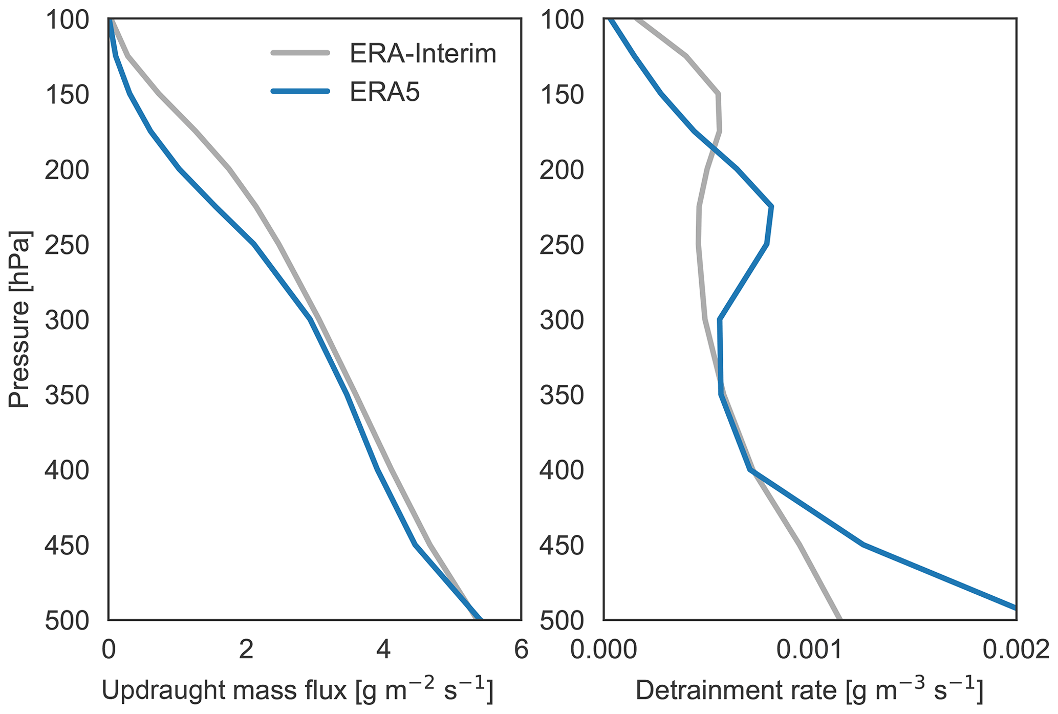
Figure A2Vertical profiles of updraught mass fluxes and fractional detrainment rates in ERA5 (blue) and ERA-Interim (grey) for 10∘ S–10∘ N during January 2010.
A3 Parameterizations of radiative transfer
Details of the radiation parameterizations and their treatments of clouds are listed in Table B1. All of the parameterizations are broadband schemes, in which the radiative spectrum is discretized into a predetermined set of spectral bands. The form of this discretization is dictated primarily by the presence of radiatively active constituents in the atmosphere and the wavelengths at which these constituents are active (e.g. Clough et al., 2005). Each band may feature parameterizations of radiative transfer due to multiple species, as well as scattering, absorption, and emission by clouds and aerosols. Radiative fluxes and heating rates (i.e. the vertical convergence of radiative fluxes) are computed by integrating across all spectral bands. ERA-Interim, JRA-55, MERRA-2, and CFSR (through 2010) all assume maximum–random overlap for cloudy columns: cloud layers that are contiguous in the vertical coordinate are assumed to have maximal overlap, and cloud layers that are not contiguous in the vertical coordinate are assumed to overlap randomly. The Monte Carlo Independent Column Approximation (McICA; Pincus et al., 2003) is used in ERA5 (with generalized overlap; Morcrette et al., 2008) and CFSv2 (with maximum–random overlap, starting from 2011; Saha et al., 2014). The introduction of McICA is therefore a potential source of discontinuity at the CFSR–CFSv2 transition. Representations of the optical properties of ice and liquid water clouds are also noted in Table B1.
Bechtold et al. (2006)Bechtold et al. (2014)Bechtold et al. (2006)Gregory et al. (2000)Xie and Zhang (2000)Hong and Pan (1998)Table A1Summary information on deep convective parameterizations used in the reanalyses. Here CAPE is convective available potential energy, PCAPE is an entraining CAPE evaluated in pressure coordinates (Bechtold et al., 2014), LCL is the lifting condensation level, ABL is the atmospheric boundary layer, and A–S stands for Arakawa–Schubert.
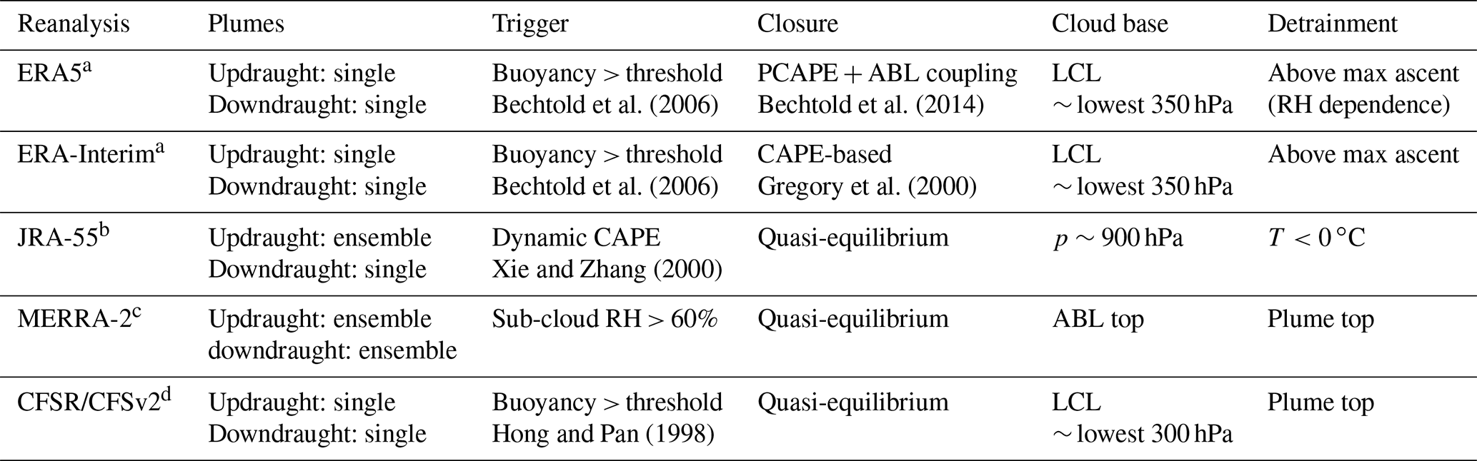
a Deep convection based on the scheme described by Tiedtke (1989). b Deep convection based on the “economical prognostic” Arakawa–Schubert scheme described by JMA (2013). c Deep convection based on the “relaxed” Arakawa–Schubert scheme described by Moorthi and Suárez (1992). d Deep convection based on the simplified Arakawa–Schubert scheme described by Pan and Wu (1995) and Moorthi et al. (2001).
As documented in Sect. 6, there is a sharp jump in HCC between the end of the original run of CFSR (December 2009) and the beginning of the CFSv2 extension (January 2011). Despite this sudden increase, changes in OLR and LWCRE around this transition were relatively small. In this appendix, we provide additional information on changes in cloud and radiation products at the CFSR–CFSv2 transition that helps to clarify some but not all of the changes in clouds and radiation. Figure B1 shows differences in zonal-mean RH and CWC between the last 4 years of CFSR (2006–2009) and the first 4 years of CFSv2 (2011–2014), while Fig. B2 shows horizontal distributions of HCC and OLR for the same periods. Figure B2d shows changes in HCC based on ISCCP HGM for the 2011–2014 mean minus the 2006–2009 mean as an illustration of natural variability between these two periods, while Fig. B2h shows changes in upward SW radiation at the TOA to further illustrate differences between the two systems.
Relative humidities near the tropical tropopause are much larger in CFSv2 (Fig. B1b) than in CFSR (Fig. B1a). Whereas CFSR produced RH near zero at 100 hPa, conditions approach saturation at this level in CFSv2. The latter better matches observations in this part of the atmosphere (e.g. Fueglistaler et al., 2009), although the mean values are somewhat larger than expected. Consistent with this increase in humidity, values of CWC are enhanced in CFSv2 relative to CFSR near the tropopause. CWCs are also much larger in CFSv2 on the flanks of the tropics but slightly reduced near the convective detrainment layer in the deep tropics. CFSR and CFSv2 do not provide vertical distributions of cloud fraction; however, the underlying models determine cloud fractions primarily as a function of CWC, with RH as a secondary factor (Appendix A1). Zonal-mean changes in the vertical distribution of cloud fraction should therefore be similar to those in CWC, with increases close to the tropopause and on the flanks of the tropics balanced against decreases in the inner tropics around 150–200 hPa. The spatial distribution of differences in cloud fraction between CFSR and CFSv2 (Fig. B2c) supports this view. In particular, the sudden jump in tropical-mean HCC seen in the time series (Fig. 14a) results primarily from large increases in cloud fraction outside of the core equatorial convective regions.
Differences in OLR between CFSR and CFSv2 are shown in Fig. B2e–g. Although the small magnitude of changes in OLR involves some measure of compensation between different regions of the tropics (e.g. increases over Africa balanced by decreases over the western Pacific warm pool), it is clear that the changes in OLR do not match those in HCC. Indeed, the bulk of the change in OLR (−1.7 W m−2) can be attributed to a decrease in the clear-sky OLR (−1.5 W m−2), which may be contributed at least in part by the changes in TTL humidity (Fig. B1c). The transition to CFSv2 involved an increase in model horizontal resolution and changes in the radiation scheme (Saha et al., 2014; Fujiwara et al., 2017), including the adoption of McICA (Appendix A3). Model tuning conducted to re-establish TOA energy balance after these changes may have smoothed out the change in OLR that would otherwise have resulted from such a large jump in HCC. In this sense, it is interesting to note an increase of 7.2 W m−2 in the net CRE between the last 4 years of CFSR and the first 4 years of CFSv2. Given the near-zero change in LWCRE (0.2 W m−2), this implies a decrease of 7.0 W m−2 in the magnitude of SWCRE (i.e. cloud albedo). This change in SWCRE was undoubtedly also impacted by model changes aimed at marine low-level clouds (Saha et al., 2014). However, the spatial distribution of decreases in upward SW flux at the TOA (Fig. B2h) indicates that reductions in planetary albedo resulted more from differences in high clouds than differences in marine stratocumulus clouds, as the latter seems to have produced regional increases in albedo.
It is perplexing that increases in HCC and upper-level CWC lead to an unchanged LWCRE and a reduced planetary albedo between CFSR and CFSv2, as increases in these cloud variables would typically be expected to strengthen both LWCRE and the planetary albedo. The flux balances match expectations internally for both CFSR and CFSv2; indeed, the net all-sky radiative flux is in good agreement with CERES EBAF (Fig. 6). It is only when we evaluate the changes at the transition that these inconsistencies crop up, implicating changes in the model. Precisely which changes to the model are responsible is unclear at present; however, both the existence of these discrepancies and the scale of the associated changes underscore our summary recommendation that users of CFSR/CFSv2 should approach any analysis spanning the transition with extreme care.
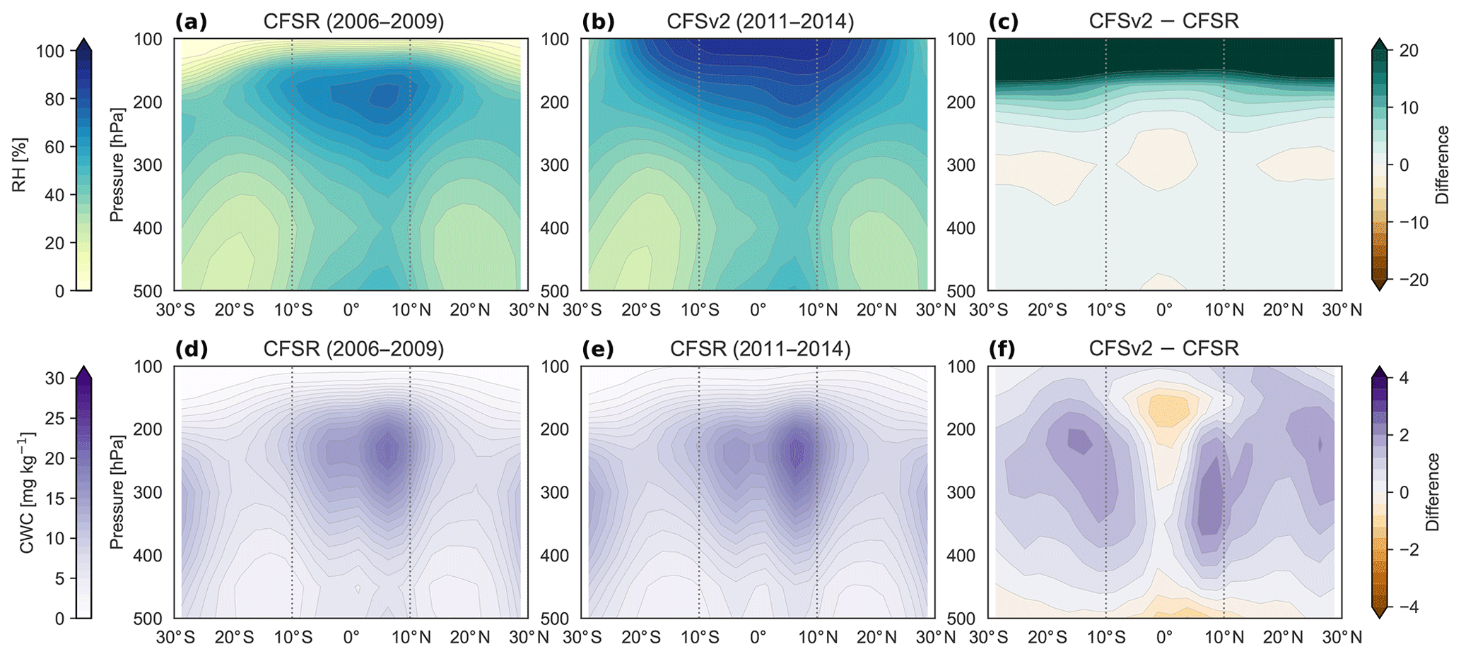
Figure B1(a–c) Zonal-mean distributions of relative humidity based on (a) the last 4 years of the original CFSR (2006–2009) and (b) the first 4 years of CFSv2 (2011–2014), along with (c) the difference between the two products (in percentage points). (d–f) As in (a–c) but for cloud water content.
Table B1Summary information on radiation parameterizations, cloud overlap, and cloud optical properties used in the reanalyses. In the column labelled “Optical properties”, L stands for liquid water clouds and I for ice clouds. Sources of cloud optical properties may differ between the LW and SW schemes. RRTMG: Rapid Radiative Transfer Model. CLIRAD.
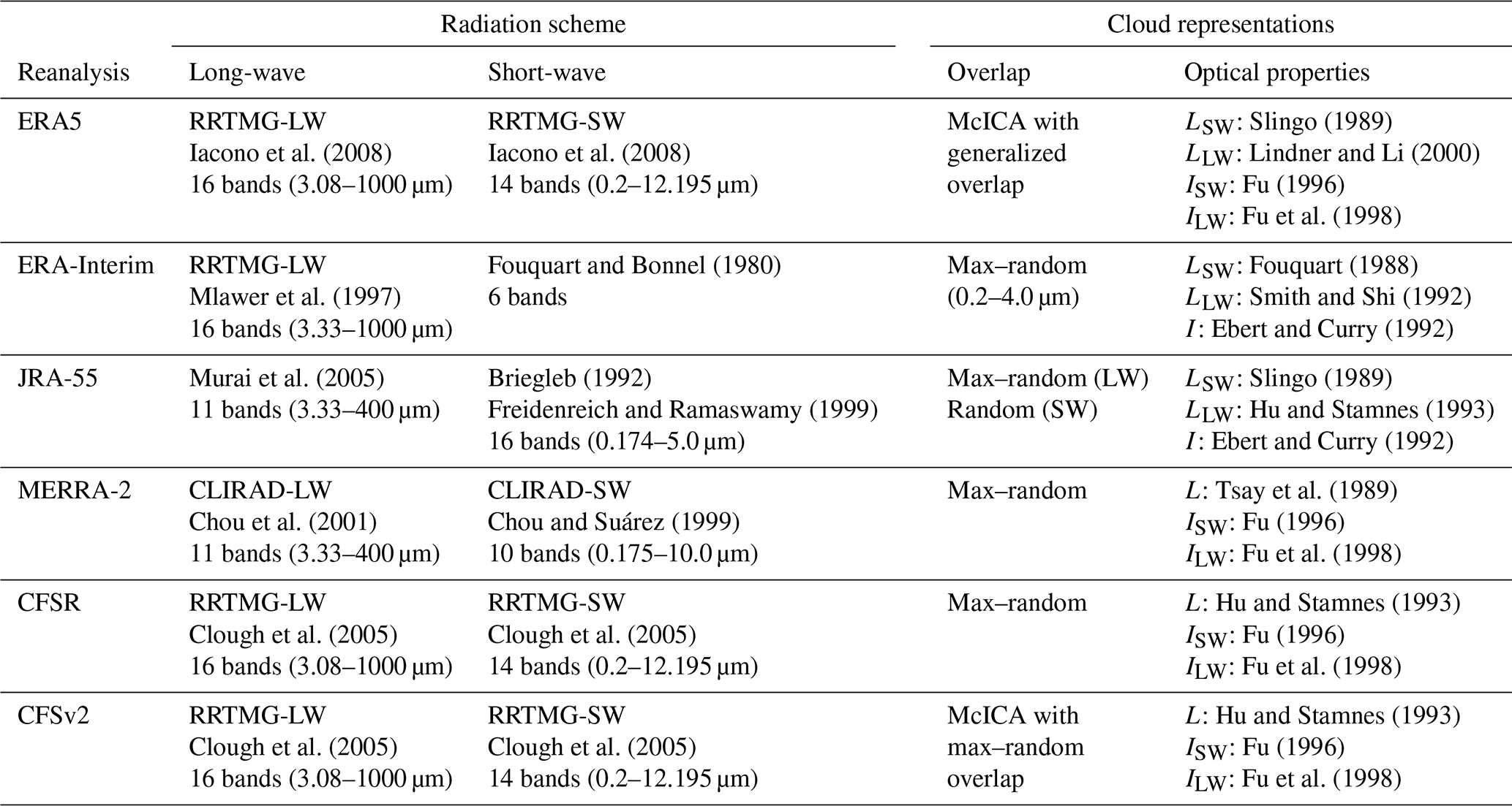
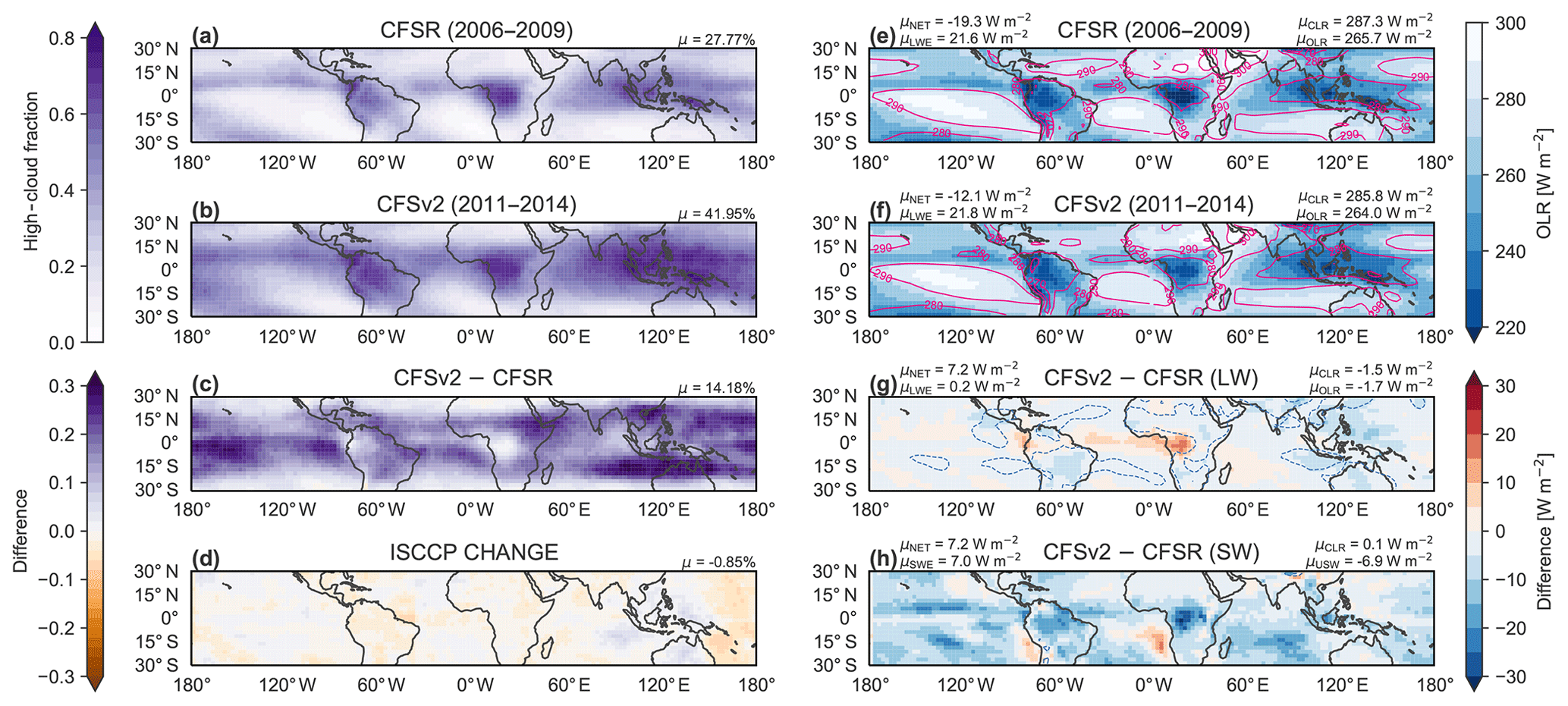
Figure B2(a–d) Distributions of high-cloud fraction based on (a) the last 4 years of the original CFSR (2006–2009) and (b) the first 4 years of CFSv2 (2011–2014), along with (c) the difference between CFSv2 and CFSR. The change in ISCCP HGM high-cloud fraction between the 2006–2009 mean and the 2011–2014 mean is shown for context in (d). (e–h) As in (a–d) but for all-sky (shading) and clear-sky (contours) OLR and with the change in all-sky upward SW flux between the 2006–2009 CFSR mean and the 2011–2014 CFSv2 mean shown in (h). Tropical-mean (30∘ S–30∘ N) values of HCC (or ΔHCC) are listed at upper right of (a) through (d). Tropical-mean values of the all-sky flux, clear-sky flux, CRE (LW or SW), and net CRE (or corresponding Δ values) are listed at the upper right (all-sky and clear-sky flux) or the upper left (CRE and net CRE) of (e) through (h).
ERA-Interim products were acquired from the public archive maintained by ECMWF (http://apps.ecmwf.int/datasets, ECMWF, 2011a, b) using the Python API (https://confluence.ecmwf.int/display/WEBAPI, ECMWF, 2018d). Daily-average heating rates and TOA fluxes were constructed from 12 h forecasts. Daily averages of all other data are from instantaneous 6-hourly products. ERA5 heating rates were also acquired from the ECMWF archive (ECMWF, 2018c) using the Python API; all other ERA5 products were acquired from the Copernicus Climate Data Store (https://cds.climate.copernicus.eu, ECMWF, 2018a, b, 2019a, b). Due to bandwidth and storage limitations, vertically resolved data from ERA5 were obtained at 3-hourly resolution, while two-dimensional data (cloud fractions and OLR) were obtained at the full hourly resolution. Daily-average heating rates and TOA fluxes were constructed from time-averaged data, while daily averages of all other variables were constructed from instantaneous outputs. JRA-55 heating rates were obtained from the NCAR Research Data Archive (RDA; https://rda.ucar.edu, JMA, 2013b); all other JRA-55 products were obtained from archives maintained by the Japan Meteorological Agency (http://jra.kishou.go.jp/JRA-55, JMA, 2013a). Daily means of heating rates and TOA fluxes were calculated from time-averaged diagnostic fields, while daily means of other variables were calculated from instantaneous outputs at the standard temporal resolution (6-hourly for vertically resolved fields; 3-hourly for high-cloud cover). CFSR and CFSv2 products were acquired exclusively through the NCAR RDA (Saha et al., 2010a, b, 2012). Daily averages of heating rates and TOA fluxes were calculated from time-averaged forecast fields; daily averages of all other variables were calculated from 6-hourly instantaneous fields. MERRA and MERRA-2 products were obtained from the NASA Goddard Earth Sciences Data and Information Services Center (https://daac.gsfc.nasa.gov, GES DISC, 2020). For MERRA we exclusively used monthly-mean IAU products (GMAO, 2008a, b). For MERRA-2 daily means we use the 3-hourly time-averaged heating rates (GMAO, 2015c) and 3-hourly instantaneous profile fields (GMAO, 2015a), both from the IAU (ASM) product set. Hourly time-averaged fields were used for high-cloud fraction and TOA radiative fluxes (GMAO, 2015b). 6-hourly analysis fields (GMAO, 2015d) were used for context and monthly-mean fields (GMAO, 2015e, f, g) were used to construct climatologies. Access dates for reanalysis products range from March 2015 to August 2019 depending on reanalysis, variable, and temporal resolution. ISCCP HGM products were acquired from the NOAA National Centers for Environmental Information (https://www.ncdc.noaa.gov/isccp, Rossow et al, 2017). CERES data were obtained from the NASA Langley Research Center Atmospheric Science Data Center (https://ceres.larc.nasa.gov, Doelling, 2017, 2019), and AIRS data were obtained from the GES DISC (AIRS Science Team and Teixeira, 2013). CloudSat–CALIPSO combined cloud fractions were provided by Jennifer Kay (personal communication, 15 December 2017), and CFMIP-GOCCP products were provided by the Institut Pierre Simon Laplace (https://climserv.ipsl.polytechnique.fr/cfmip-obs, CFMIP, 2018). CloudSat 2C-ICE products (CloudSat Data Processing Center, 2019) were acquired and processed via the AERIS Data Portal (https://www.aeris-data.fr, AERIS, 2020). NOAA Interpolated OLR data were acquired from the NOAA/OAR/ESRL Physical Science Division, Boulder, Colorado, USA (https://www.esrl.noaa.gov/psd, NCAR/NOAA, 1996). The NASA/GEWEX SRB data were acquired from the NASA Langley Atmospheric Science Data Center (https://gewex-srb.larc.nasa.gov, SRB Science Team, 2012).
JSW and XS conducted the analysis and wrote the initial draft. BL and XZ provided data and helped to interpret the results. PK, KK, AM, ST, and GJZ suggested additional analyses and revisions for the paper. AM checked and clarified key aspects of MERRA-2.
The authors declare that they have no conflict of interest.
This article is part of the special issue “The SPARC Reanalysis Intercomparison Project (S-RIP) (ACP/ESSD inter-journal SI)”. It is not associated with a conference.
We thank Peter Bechtold from ECMWF, Yayoi Harada and Ryoji Nagasawa from the JMA Meteorological Research Institute, and Kris Wargan from NASA GMAO for help in clarifying aspects of the reanalysis data and Yi Huang and an anonymous reviewer for comments and suggestions that have greatly improved the paper. We are also grateful to Xianglei Huang for advice on OLR data and radiative transfer models, to Jennifer Kay for providing the CloudSat–CALIPSO data, and to Yi Qin and Xiaolu Yan for helpful discussions. A condensed version of this material has been prepared for Section 8 of the S-RIP report. We thank Masatomo Fujiwara, Gloria Manney, and Lesley Gray for their leadership of this activity and all S-RIP participants for their contributions.
This research has been supported by the Ministry of Science and Technology of the People's Republic of China (grant no. 2017YFA0603902), the National Natural Science Foundation of China (grant no. 41761134097), the Deutsche Forschungsgemeinschaft (grant no. 392169209), and the Ministry of Science and Technology of the People's Republic of China (grant no. 2017YFA0603902).
This paper was edited by Peter Haynes and reviewed by Yi Huang and one anonymous referee.
Abalos, M., Legras, B., Ploeger, F., and Randel, W. J.: Evaluating the advective Brewer–Dobson circulation in three reanalyses for the period 1979–2012, J. Geophys. Res.-Atmos., 120, 7534–7554, https://doi.org/10.1002/2015JD023182, 2015. a
AERIS: Données et Services Pour l'Atmosphère, available at: https://www.aeris-data.fr, last access: 24 July 2020. a
Anber, U., Wang, S., and Sobel, A.: Response of atmospheric convection to vertical wind shear: Cloud-system-resolving simulations with parameterized large-scale circulation. Part II: Effect of interactive radiation, J. Atmos. Sci., 73, 199–209, https://doi.org/10.1175/JAS-D-15-0151.1, 2016. a
Arakawa, A. and Schubert, W. H.: Interaction of a cumulus cloud ensemble with the large-scale environment, part I, J. Atmos. Sci., 31, 674–701, 1974. a, b
Bacmeister, J. T. and Stephens, G. L.: Spatial statistics of likely convective clouds in CloudSat data, J. Geophys. Res.-Atmos., 116, D04104, https://doi.org/10.1029/2010JD014444, 2011. a, b
Bacmeister, J. T., Suárez, M. J., and Robertson, F. R.: Rain reevaporation, boundary layer–convection interactions, and Pacific rainfall patterns in an AGCM, J. Atmos. Sci., 63, 3383–3403, https://doi.org/10.1175/JAS3791.1, 2006. a, b
Bannister, R. N., Chipilski, H. G., and Martinez-Alvarado, O.: Techniques and challenges in the assimilation of atmospheric water observations for numerical weather prediction towards convective scales, Q. J. Roy. Meteorol. Soc., 146, 1–48, https://doi.org/10.1002/qj.3652, 2020. a
Bechtold, P., Chaboureau, J.-P., Beljaars, A., Betts, A. K., Köhler, M., Miller, M., and Redelsperger, J.-L.: The simulation of the diurnal cycle of convective precipitation over land in a global model, Q. J. Roy. Meteorol. Soc., 130, 3119–3137, https://doi.org/10.1256/qj.03.103, 2006. a, b, c
Bechtold, P., Köhler, M., Jung, T., Doblas-Reyes, F., Leutbecher, M., Rodwell, M. J., Vitart, F., and Balsamo, G.: Advances in simulating atmospheric variability with the ECMWF model: From synoptic to decadal time-scales, Q. J. Roy. Meteorol. Soc., 134, 1337–1351, https://doi.org/10.1002/qj.289, 2008. a, b, c, d, e
Bechtold, P., Semane, N., Lopez, P., Chaboureau, J.-P., Beljaars, A., and Bormann, N.: Representing Equilibrium and Nonequilibrium Convection in Large-Scale Models, J. Atmos. Sci., 71, 734–753, https://doi.org/10.1175/JAS-D-13-0163.1, 2014. a, b, c, d, e, f, g, h
Bloom, S. C.: Data assimilation using incremental analysis updates, Mon. Weather Rev., 124, 1256–1271, 1996. a
Bodas-Salcedo, A., Webb, M. J., Bony, S., Chepfer, H., Dufresne, J. L., Klein, S. A., Zhang, Y., Marchand, R., Haynes, J. M., and Pincus, R.: COSP: Satellite simulation software for model assessment, B. Am. Meteorol. Soc., 92, 1023–1043, https://doi.org/10.1175/2011BAMS2856.1, 2015. a, b
Bolton, D.: The computation of equivalent potential temperature, Mon. Weather Rev., 108, 1046–1053, 1980. a
Bony, S., Stevens, B., Frierson, D. M. W., Jakob, C., Kageyama, M., Pincus, R., Shepherd, T. G., Sherwood, S. C., Siebesma, A. P., Sobel, A. H., Watanabe, M., and Webb, M. J.: Clouds, circulation, and climate sensitivity, Nat. Geosci., 8, 261–268, https://doi.org/10.1038/ngeo2398, 2015. a
Briegleb, B. P.: Delta-Eddington approximation for solar radiation in the NCAR community climate model, J. Geophys. Res.-Atmos., 97, 7603–7612, https://doi.org/10.1029/92JD00291, 1992. a
Cao, G. and Zhang, G. J.: Role of vertical structure of convective heating in MJO simulation in NCAR CAM5.3, J. Climate, 30, 7423–7439, https://doi.org/10.1175/JCLI-D-16-0913.1, 2017. a
Carr, M. T. and Bretherton, C. S.: Convective momentum transport over the tropical Pacific: Budget estimates, J. Atmos. Sci., 58, 1673–1693, 2001. a
Chepfer, H., Bony, S., Winker, D., Cesana, G., Dufresne, J. L., Minnis, P., Stubenrauch, C. J., and Zeng, S.: The GCM‐Oriented CALIPSO Cloud Product (CALIPSO‐GOCCP), J. Geophys. Res.-Atmos., 115, D00H16, https://doi.org/10.1029/2009JD012251, 2010. a, b, c, d
Chou, M.-D. and Suárez, M.: A solar radiation parameterization for atmospheric studies, Technical Report Series on Global Modeling and Data Assimilation, No. 15, NASA/TM-1999-104606, NASA, Greenbelt, Maryland, available at: https://ntrs.nasa.gov/search.jsp?R=19990060930 (last access: August 2018), 1999. a
Chou, M.-D., Suárez, M., Liang, X.-Z., and Yan, M. M.-H.: A thermal infrared radiation parameterization for atmospheric studies, Technical Report Series on Global Modeling and Data Assimilation, No. 19, NASA/TM-2001-104606, NASA, Greenbelt, Maryland, available at: https://ntrs.nasa.gov/search.jsp?R=20010072848 (last access: August 2018), 2001. a
Clough, S., Shephard, M., Mlawer, E., Delamere, J., Iacono, M., Cady-Pereira, K., Boukabara, S., and Brown, P.: Atmospheric radiative transfer modeling: a summary of the AER codes, J. Quant. Spectrosc. Ra., 91, 233–244, https://doi.org/10.1016/j.jqsrt.2004.05.058, 2005. a, b, c, d, e
Cloud Feedback Model Intercomparison Project (CFMIP): GCM-Oriented CALIPSO Cloud Product: 3D Cloud Fraction, version 3.1.2, available at: https://climserv.ipsl.polytechnique.fr/cfmip-obs/ (last access: 15 July 2020), 2018. a
CloudSat Data Processing Center: Cloudsat and CALIPSO Ice Cloud Property Product (2C-ICE), P1_R05, available at: http://www.cloudsat.cira.colostate.edu/data-products/level-2c/2c-ice (last access: 21 July 2020), 2019. a
Corti, T., Luo, B. P., Peter, T., Vömel, H., and Fu, Q.: Mean radiative energy balance and vertical mass fluxes in the equatorial upper troposphere and lower stratosphere, Geophys. Res. Lett., 32, L06802, https://doi.org/10.1029/2004GL021889, 2005. a, b
Courtier, P., Thépaut, J.-N., and Hollingsworth, A.: A strategy for operational implementation of 4D-Var, using an incremental approach, Q. J. Roy. Meteorol. Soc., 120, 1367–1387, https://doi.org/10.1002/qj.49712051912, 1994. a
Dai, A., Karl, T. R., Sun, B., and Trenberth, K. E.: Recent trends in cloudiness over the United States: A tale of monitoring inadequacies, B. Am. Meteorol. Soc., 87, 597–606, https://doi.org/10.1175/BAMS-87-5-597, 2006. a
Davis, S. M., Hegglin, M. I., Fujiwara, M., Dragani, R., Harada, Y., Kobayashi, C., Long, C., Manney, G. L., Nash, E. R., Potter, G. L., Tegtmeier, S., Wang, T., Wargan, K., and Wright, J. S.: Assessment of upper tropospheric and stratospheric water vapor and ozone in reanalyses as part of S-RIP, Atmos. Chem. Phys., 17, 12743–12778, https://doi.org/10.5194/acp-17-12743-2017, 2017. a, b, c
Dee, D. P., Uppala, S. M., Simmons, A. J., Berrisford, P., Poli, P., Kobayashi, S., Andrae, U., Balmaseda, M. A., Balsamo, G., and Bauer, P.: The ERA‐Interim reanalysis: configuration and performance of the data assimilation system, Q. J. Roy. Meteorol. Soc., 137, 553–597, https://doi.org/10.1002/qj.828, 2011. a, b
Del Genio, A. D., Yao, M.-S., Kovari, W., and Lo, K. K.-W.: A prognostic cloud water parameterization for global climate models, J. Climate, 9, 270–304, 1996. a
Deng, M., Mace, G. G., Wang, Z., and Berry, E.: CloudSat 2C-ICE product update with a new Ze parameterization in lidar-only region, J. Geophys. Res.-Atmos., 120, 12198–12208, https://doi.org/10.1002/2015JD023600, 2015. a, b
Dessler, A. E.: A determination of the cloud feedback from climate variations over the past decade, Science, 330, 1523–1527, https://doi.org/10.1126/science.1192546, 2010. a
Dessler, A. E. and Yang, P.: The distribution of tropical thin cirrus clouds inferred from Terra MODIS data, J. Climate, 16, 1241–1247, 2003. a
Dessler, A. E., Schoeberl, M. R., Wang, T., Davis, S. M., Rosenlof, K. H., and Vernier, J.-P.: Variations of stratospheric water vapor over the past three decades, J. Geophys. Res.-Atmos., 119, 12588–12598, https://doi.org/10.1002/2014JD021712, 2014. a
Doelling, D. R.: CERES SYN1DEG-DAYTerra+Aqua – Edition 4A, NASA Atmospheric Science Data Center (ASDC), Hampton, VA, USA, https://doi.org/10.5067/terra+aqua/ceres/syn1degday_l3.004a, 2017. a, b, c, d
Doelling, D. R.: CERES Energy Balanced and Filled (EBAF) TOA and Surface Monthly means data in netCDF Edition 4.1, NASA Atmospheric Science Data Center (ASDC), Hampton, VA, USA, https://doi.org/10.5067/TERRA-AQUA/CERES/EBAF_L3B.004.1, 2019. a, b, c
Doelling, D. R., Scarino, B. R., Morstad, D., Gopalan, A., Bhatt, R., Lukashin, C., and Minnis, P.: The intercalibration of geostationary visible imagers using operational hyperspectral SCIAMACHY radiances, IEEE T. Geosci. Remote, 51, 1245–1254, https://doi.org/10.1109/TGRS.2012.2227760, 2013. a
Dolinar, E. K., Dong, X., and Xi, B.: Evaluation and intercomparison of clouds, precipitation, and radiation budgets in recent reanalyses using satellite-surface observations, Clim. Dynam., 46, 2123–2144, https://doi.org/10.1007/s00382-015-2693-z, 2016. a, b
Ebert, E. E. and Curry, J. A.: A parameterization of ice cloud optical properties for climate models, J. Geophys. Res.-Atmos., 97, 3831–3836, https://doi.org/10.1029/91JD02472, 1992. a, b
Emanuel, K. A.: Atmospheric Convection, Oxford University Press, New York, 580 pp., 1994. a
Emanuel, K. A., Neelin, D. J., and Bretherton, C. S.: On large-scale circulations in convecting atmospheres, Q. J. Roy. Meteorol. Soc., 120, 1111–1143, https://doi.org/10.1002/qj.49712051902, 1994. a
European Centre for Medium-Range Weather Forecasts (ECMWF): ERA-Interim Public Archive, ECMWF, Shinfield Park, Reading, UK, available at: https://apps.ecmwf.int/datasets/data/interim-full-daily (last access: 15 July 2020), 2011a. a
European Centre for Medium-Range Weather Forecasts (ECMWF): ERA-Interim Archive Catalogue, ECMWF, Shinfield Park, Reading, UK, available at: https://apps.ecmwf.int/archive-catalogue/?class=ei (last access: 15 July 2020), 2011b. a
European Centre for Medium-Range Weather Forecasts (ECMWF): ERA5 hourly data on single levels from 1979 to present, Copernicus Climate Data Store, Reading, UK, https://doi.org/10.24381/cds.adbb2d47, 2018a. a
European Centre for Medium-Range Weather Forecasts (ECMWF): ERA5 hourly data on pressure levels from 1979 to present, Copernicus Climate Data Store, Reading, UK, https://doi.org/10.24381/cds.bd0915c6, 2018b. a
European Centre for Medium-Range Weather Forecasts (ECMWF): ERA5 Catalogue, ECMWF, Shinfield Park, Reading, UK, available at: https://apps.ecmwf.int/data-catalogues/era5 (last access: 15 July 2020), 2018c. a
European Centre for Medium-Range Weather Forecasts (ECMWF): ECMWF Web API, Shinfield Park, Reading, UK, available at: https://confluence.ecmwf.int/display/WEBAPI/ (last access: 15 July 2020), 2018d. a
European Centre for Medium-Range Weather Forecasts (ECMWF): ERA5 monthly averaged data on single levels from 1979 to present, Copernicus Climate Data Store, Reading, UK, https://doi.org/10.24381/cds.f17050d7, 2019a. a
European Centre for Medium-Range Weather Forecasts (ECMWF): ERA5 monthly averaged data on pressure levels from 1979 to present, Copernicus Climate Data Store, Reading, UK, https://doi.org/10.24381/cds.6860a573, 2019b. a
Fiehn, A., Quack, B., Hepach, H., Fuhlbrügge, S., Tegtmeier, S., Toohey, M., Atlas, E., and Krüger, K.: Delivery of halogenated very short-lived substances from the west Indian Ocean to the stratosphere during the Asian summer monsoon, Atmos. Chem. Phys., 17, 6723–6741, https://doi.org/10.5194/acp-17-6723-2017, 2017. a
Folkins, I., Loewenstein, M., Podolske, J., Oltmans, S. J., and Proffitt, M.: A barrier to vertical mixing at 14 km in the tropics: Evidence from ozonesondes and aircraft measurements, J. Geophys. Res.-Atmos., 104, 22095–22102, https://doi.org/10.1029/1999JD900404, 1999. a
Folkins, I., Braun, C., Thompson, A. M., and Witte, J.: Tropical ozone as an indicator of deep convection, J. Geophys. Res.-Atmos., 107, ACH 13-1–ACH 13-10, https://doi.org/10.1029/2001JD001178, 2002. a
Forbes, R. M., Tompkins, A. M., and Untch, A.: A new prognostic bulk microphysics scheme for the IFS, Technical Memorandum 649, ECMWF, Shinfield Park, Reading, UK, https://doi.org/10.21957/bf6vjvxk, 2011. a
Fouquart, Y.: Radiative transfer in climate models, in: Physically-Based Modelling and Simulation of Climate and Climatic Change: Part 1, edited by Schlesinger, M. E., Springer Netherlands, Dordrecht, 223–283, https://doi.org/10.1007/978-94-009-3041-4_5, 1988. a
Fouquart, Y. and Bonnel, B.: Computation of solar heating of the Earth's atmosphere: a new parameterization, Beitr. Phys., 53, 35–62, 1980. a
Fowler, L. D., Wielicki, B. A., Randall, D. A., Branson, M. D., Gibson, G. G., and Denn, F. M.: Use of a GCM to explore sampling issues in connection with satellite remote sensing of the Earth radiation budget, J. Geophys. Res.-Atmos., 105, 20757–20772, https://doi.org/10.1029/2000JD900239, 2000. a
Freidenreich, S. M. and Ramaswamy, V.: A new multiple-band solar radiative parameterization for general circulation models, J. Geophys. Res.-Atmos., 104, 31389–31409, https://doi.org/10.1029/1999JD900456, 1999. a
Fu, Q.: An accurate parameterization of the solar radiative properties of cirrus clouds for climate models, J. Climate, 9, 2058–2082, 1996. a, b, c, d
Fu, Q., Yang, P., and Sun, W. B.: An accurate parameterization of the infrared radiative properties of cirrus clouds for climate models, J. Climate, 11, 2223–2237, 1998. a, b, c, d
Fu, R., Liu, W. T., and Dickinson, R. E.: Response of tropical clouds to the interannual variation of sea surface temperature, J. Climate, 9, 616–634, 1996. a
Fueglistaler, S. and Fu, Q.: Impact of clouds on radiative heating rates in the tropical lower stratosphere, J. Geophys. Res.-Atmos., 111, D23202, https://doi.org/10.1029/2006JD007273, 2006. a, b, c
Fueglistaler, S., Dessler, A. E., Dunkerton, T. J., Folkins, I., Fu, Q., and Motte, P. W.: Tropical tropopause layer, Rev. Geophys., 47, RG1004, https://doi.org/10.1029/2008RG000267, 2009. a, b, c
Fujiwara, M., Wright, J. S., Manney, G. L., Gray, L. J., Anstey, J., Birner, T., Davis, S., Gerber, E. P., Harvey, V. L., Hegglin, M. I., Homeyer, C. R., Knox, J. A., Krüger, K., Lambert, A., Long, C. S., Martineau, P., Molod, A., Monge-Sanz, B. M., Santee, M. L., Tegtmeier, S., Chabrillat, S., Tan, D. G. H., Jackson, D. R., Polavarapu, S., Compo, G. P., Dragani, R., Ebisuzaki, W., Harada, Y., Kobayashi, C., McCarty, W., Onogi, K., Pawson, S., Simmons, A., Wargan, K., Whitaker, J. S., and Zou, C.-Z.: Introduction to the SPARC Reanalysis Intercomparison Project (S-RIP) and overview of the reanalysis systems, Atmos. Chem. Phys., 17, 1417–1452, https://doi.org/10.5194/acp-17-1417-2017, 2017. a, b, c, d, e, f, g, h
Fusina, F., Spichtinger, P., and Lohmann, U.: Impact of ice supersaturated regions and thin cirrus on radiation in the midlatitudes, J. Geophys. Res.-Atmos., 112, D24S14, https://doi.org/10.1029/2007JD008449, 2007. a
Gelaro, R., McCarty, W., Suárez, M. J., Todling, R., Molod, A., Takacs, L., Randles, C., Darmenov, A., Bosilovich, M. G., Reichle, R., Wargan, K., Coy, L., Cullather, R., Draper, C., Akella, S., Buchard, V., Conaty, A., da Silva, A., Gu, W., Kim, G.-K., Koster, R., Lucchesi, R., Merkova, D., Nielsen, J. E., Partyka, G., Pawson, S., Putman, W., Rienecker, M., Schubert, S. D., Sienkiewicz, M., and Zhao, B.: The Modern-Era Retrospective Analysis for Research and Applications, Version 2 (MERRA-2), J. Climate, 30, 5419–5454, https://doi.org/10.1175/JCLI-D-16-0758.1, 2017. a, b
Geller, M. A., Zhou, T., and Yuan, W.: The QBO, gravity waves forced by tropical convection, and ENSO, J. Geophys. Res.-Atmos., 121, 8886–8895, https://doi.org/10.1002/2015JD024125, 2016. a
GES DISC: Goddard Earth Sciences Data and Information Services Center, available at: https://daac.gsfc.nasa.gov, last access: 24 July 2020. 2020. a
Gettelman, A., Forster, P. M. D. F., Fujiwara, M., Fu, Q., Vömel, H., Gohar, L. K., Johanson, C., and Ammerman, M.: Radiation balance of the tropical tropopause layer, J. Geophys. Res.-Atmos., 109, D07103, https://doi.org/10.1029/2003JD004190, 2004. a
Global Modeling and Assimilation Office (GMAO): instM_3d_asm_Cp: MERRA 3D IAU State, Meteorology Monthly Mean V5.2.0, Goddard Earth Sciences Data and Information Services Center (GES DISC), Greenbelt, MD, USA, https://doi.org/10.5067/YX0AVASQRTNW, 2008a. a
Global Modeling and Assimilation Office (GMAO): tavgM_3d_rad_Cp: MERRA 3D IAU Diagnostic, Radiation, Monthly Mean V5.2.0, Goddard Earth Sciences Data and Information Services Center (GES DISC), Greenbelt, MD, USA, https://doi.org/10.5067/7SCF81BU67P5, 2008b. a
Global Modeling and Assimilation Office (GMAO): MERRA-2 inst3_3d_asm_Np: 3d,3-Hourly,Instantaneous,Pressure-Level, Assimilation, Assimilated Meteorological Fields V5.12.4, Goddard Earth Sciences Data and Information Services Center (GES DISC), Greenbelt, MD, USA, https://doi.org/10.5067/QBZ6MG944HW0, 2015a. a
Global Modeling and Assimilation Office (GMAO): MERRA-2 tavg1_2d_rad_Nx: 2d,1-Hourly,Time-Averaged,Single-Level, Assimilation, Radiation Diagnostics V5.12.4, Goddard Earth Sciences Data and Information Services Center (GES DISC), Greenbelt, MD, USA, https://doi.org/10.5067/Q9QMY5PBNV1T, 2015b. a
Global Modeling and Assimilation Office (GMAO): MERRA-2 tavg3_3d_rad_Np: 3d,3-Hourly,Time-Averaged,Pressure-Level, Assimilation, Radiation Diagnostics V5.12.4, Goddard Earth Sciences Data and Information Services Center (GES DISC), Greenbelt, MD, USA, https://doi.org/10.5067/3UGE8WQXZAOK, 2015c. a
Global Modeling and Assimilation Office (GMAO): MERRA-2 inst6_3d_ana_Np: 3d,6-Hourly,Instantaneous,Pressure-Level, Analysis, Analyzed Meteorological Fields V5.12.4, Goddard Earth Sciences Data and Information Services Center (GES DISC), Greenbelt, MD, USA, https://doi.org/10.5067/A7S6XP56VZWS, 2015d. a
Global Modeling and Assimilation Office (GMAO): MERRA-2 instM_3d_asm_Np: 3d,Monthly mean,Instantaneous,Pressure-Level, Assimilation, Assimilated Meteorological Fields V5.12.4, Goddard Earth Sciences Data and Information Services Center (GES DISC), Greenbelt, MD, USA, https://doi.org/10.5067/2E096JV59PK7, 2015e. a
Global Modeling and Assimilation Office (GMAO): MERRA-2 tavgM_2d_rad_Nx: 2d,Monthly mean,Time-Averaged,Single-Level, Assimilation, Radiation Diagnostics V5.12.4, Goddard Earth Sciences Data and Information Services Center (GES DISC), Greenbelt, MD, USA, https://doi.org/10.5067/OU3HJDS973O0, 2015f. a
Global Modeling and Assimilation Office (GMAO): MERRA-2 tavgM_3d_rad_Np: 3d, Monthly mean,Time-Averaged,Pressure-Level, Assimilation, Radiation Diagnostics V5.12.4, Goddard Earth Sciences Data and Information Services Center (GES DISC), Greenbelt, MD, USA, https://doi.org/10.5067/H3YGROBVBGFJ, 2015g. a
Gregory, D., Morcrette, J.-J., Jacob, C., Beljaars, A. C. M., and Stockdale, T.: Revision of convection, radiation and cloud schemes in the ECMWF integrated forecast system, Q. J. Roy. Meteorol. Soc., 126, 1685–1710, https://doi.org/10.1002/qj.49712656607, 2000. a
Hartmann, D. L. and Larson, K.: An important constraint on tropical cloud – climate feedback, Geophys. Res. Lett., 29, 1951, https://doi.org/10.1029/2002GL015835, 2002. a
Hartmann, D. L. and Michelsen, M. L.: Large-scale effects on the regulation of tropical sea surface temperature, J. Climate, 6, 2049–2062, 1993. a
Hearty, T. J., Savtchenko, A., Tian, B., Fetzer, E., Yung, Y. L., Theobald, M., Vollmer, B., Fishbein, E., and Won, Y.: Estimating sampling biases and measurement uncertainties of AIRS/AMSU‐A temperature and water vapor observations using MERRA reanalysis, J. Geophys. Res.-Atmos., 119, 2725–2741, https://doi.org/10.1002/2013JD021205, 2014. a
Hersbach, H., de Rosnay, P., Bell, B., Schepers, D., Simmons, A., Soci, C., Abdalla, S., Alonso-Balmaseda, M., Balsamo, G., Bechtold, P., Berrisford, P., Bidlot, J.-R., de Boisséson, E., Bonavita, M., Browne, P., Buizza, R., Dahlgren, P., Dee, D., Dragani, R., Diamantakis, M., Flemming, J., Forbes, R., Geer, A. J., Haiden, T., Hólm, E., Haimberger, L., Hogan, R., Horányi, A., Janiskova, M., Laloyaux, P., Lopez, P., Munoz-Sabater, J., Peubey, C., Radu, R., Richardson, D., Thépaut, J.-N., Vitart, F., Yang, X., Zsótér, E., and Zuo, H.: Operational global reanalysis: progress, future directions and synergies with NWP, ERA Report Series 27, ECMWF, Shinfield Park, Reading, UK, https://doi.org/10.21957/tkic6g3wm, 2018. a
Hersbach, H., Bell, B., Berrisford, P., Hirahara, S., Horányi, A., Muñoz-Sabater, J., Nicolas, J., Peubey, C., Radu, R., Schepers, D., Simmons, A., Soci, C., Abdalla, S., Abellan, X., Balsamo, G., Bechtold, P., Biavati, G., Bidlot, J., Bonavita, M., De Chiara, G., Dahlgren, P., Dee, D., Diamantakis, M., Dragani, R., Flemming, J., Forbes, R., Fuentes, M., Geer, A., Haimberger, L., Healy, S., Hogan, R. J., Hólm, E., Janisková, M., Keeley, S., Laloyaux, P., Lopez, P., Lupu, C., Radnoti, G., de Rosnay, P., Rozum, I., Vamborg, F., Villaume, S., and Thépaut, J.-N.: The ERA5 Global Reanalysis, Q. J. Roy. Meteorol. Soc., https://doi.org/10.1002/qj.3803, in press, 2020. a, b
Hoffmann, L., Günther, G., Li, D., Stein, O., Wu, X., Griessbach, S., Heng, Y., Konopka, P., Müller, R., Vogel, B., and Wright, J. S.: From ERA-Interim to ERA5: the considerable impact of ECMWF's next-generation reanalysis on Lagrangian transport simulations, Atmos. Chem. Phys., 19, 3097–3124, https://doi.org/10.5194/acp-19-3097-2019, 2019. a
Hong, S.-Y. and Pan, H.-L.: Convective trigger function for a mass-flux cumulus parameterization scheme, Mon. Weather Rev., 126, 2599–2620, 1998. a, b
Hu, Y. X. and Stamnes, K.: An accurate parameterization of the radiative properties of water clouds suitable for use in climate models, J. Climate, 6, 728–742, 1993. a, b, c
Huang, Y. and Ramaswamy, V.: Evolution and trend of the outgoing longwave radiation spectrum, J. Climate, 22, 4637–4651, https://doi.org/10.1175/2009JCLI2874.1, 2009. a
Iacono, M. J., Delamere, J. S., Mlawer, E. J., Shephard, M. W., Clough, S. A., and Collins, W. D.: Radiative forcing by long-lived greenhouse gases: Calculations with the AER radiative transfer models, J. Geophys. Res.-Atmos., 113, D13103, https://doi.org/10.1029/2008JD009944, 2008. a, b
Japan Meteorological Agency (JMA): JRA-55 Monthly, 6-hourly and 3-hourly data, JMA Data Dissemination System (JDDS), Tokyo, Japan, available at: https://jra.kishou.go.jp/index.html (last access: 15 July 2020), 2013a. a
Japan Meteorological Agency (JMA): JRA-55: Japanese 55-year Reanalysis, Daily 3-Hourly and 6-Hourly Data, Research Data Archive at the National Center for Atmospheric Research, Computational and Information Systems Laboratory, Boulder, CO, USA, https://doi.org/10.5065/D6HH6H41, 2013b. a
Jiang, J. H., Livesey, N. J., Su, H., Neary, L., McConnell, J. C., and Richards, N. A. D.: Connecting surface emissions, convective uplifting, and long-range transport of carbon monoxide in the upper troposphere: New observations from the Aura Microwave Limb Sounder, Geophys. Res. Lett., 34, L18812, https://doi.org/10.1029/2007GL030638, 2007. a
JMA: Outline of the operational numerical weather prediction at the Japan Meteorological Agency, Tech. rep., Japan Meteorological Agency, Tokyo, available at: http://www.jma.go.jp/jma/jma-eng/jma-center/nwp/outline2013-nwp/index.htm (last access: 15 July 2020), 2013. a, b, c
Johnson, R. H., Rickenbach, T. M., Rutledge, S. A., Ciesielski, P. E., and Schubert, W. H.: Trimodal characteristics of tropical convection, J. Climate, 12, 2397–2418, 1999. a
Kawai, H. and Inoue, T.: A simple parameterization scheme for subtropical marine stratocumulus, SOLA, 2, 17–20, https://doi.org/10.2151/sola.2006-005, 2006. a
Kay, J. E. and Gettelman, A.: Cloud influence on and response to seasonal Arctic sea ice loss, J. Geophys. Res.-Atmos., 114, D18204, https://doi.org/10.1029/2009JD011773, 2009. a, b, c, d
Kim, J., Randel, W. J., and Birner, T.: Convectively driven tropopause-level cooling and its influences on stratospheric moisture, J. Geophys. Res.-Atmos., 123, 590–606, https://doi.org/10.1002/2017JD027080, 2017. a
Kobayashi, S., Ota, Y., Harada, Y., Ebita, A., Moriya, M., Onoda, H., Onogi, K., Kamahori, H., Kobayashi, C., Endo, H., Miyaoka, K., and Takahashi, K.: The JRA-55 Reanalysis: General Specifications and Basic Characteristics, J. Meteorol. Soc. Jpn., 93, 5–48, https://doi.org/10.2151/jmsj.2015-001, 2015. a, b
Kolly, A. and Huang, Y.: The radiative feedback during the ENSO cycle: observations versus models, J. Geophys. Res.-Atmos., 123, 9097–9108, https://doi.org/10.1029/2018JD028401, 2018. a
Kosaka, Y. and Xie, S.: Recent global-warming hiatus tied to equatorial Pacific surface cooling, Nature, 501, 403–407, https://doi.org/10.1038/nature12534, 2013. a
Lane, T. P. and Moncrieff, M. W.: Stratospheric gravity waves generated by multiscale tropical convection, J. Atmos. Sci., 65, 2598–2614, https://doi.org/10.1175/2007JAS2601.1, 2008. a
L'Ecuyer, T. S., Wood, N. B., Haladay, T., Stephens, G. L., and Stackhouse Jr., P. W.: Impact of clouds on atmospheric heating based on the R04 CloudSat fluxes and heating rates data set, J. Geophys. Res.-Atmos., 113, D00A15, https://doi.org/10.1029/2008JD009951, 2008. a
LeMone, M. A., Barnes, G. M., and Zipser, E. J.: Momentum flux by lines of cumulonimbus over the tropical oceans, J. Atmos. Sci., 41, 1914–1932, 1984. a
Li, J., Mao, J., and Wang, F.: Comparative study of five current reanalyses in characterizing total cloud fraction and top‐of‐the‐atmosphere cloud radiative effects over the Asian monsoon region, Int. J. Climatol., 37, 5047–2741, https://doi.org/10.1002/joc.5143, 2017. a
Li, J.-L. F., Waliser, D. E., Chen, W.-T., Guan, B., Kubar, T., Stephens, G., Ma, H.-Y., Deng, M., Donner, L., Seman, C., and Horowitz, L.: An observationally based evaluation of cloud ice water in CMIP3 and CMIP5 GCMs and contemporary reanalyses using contemporary satellite data, J. Geophys. Res.-Atmos., 117, D16105, https://doi.org/10.1029/2012JD017640, 2012. a
Li, J.-L. F., Waliser, D. E., Stephens, G., and Lee, S.: Characterizing and understanding cloud ice and radiation budget biases in global climate models and reanalysis, Meteorol. Monogr., 56, 13.1–13.20, https://doi.org/10.1175/AMSMONOGRAPHS-D-15-0007.1, 2016. a
Lim, Y.-K., Schubert, S. D., Reale, O., Lee, M.-I., Molod, A. M., and Suárez, M. J.: Sensitivity of tropical cyclones to parameterized convection in the NASA GEOS-5 model, J. Climate, 28, 551–573, https://doi.org/10.1175/JCLI-D-14-00104.1, 2015. a
Lindner, T. H. and Li, J.: Parameterization of the optical properties for water clouds in the infrared, J. Climate, 13, 1797–1805, 2000. a
Loeb, N. G., Rose, F. G., Kato, S., Rutan, D. A., Su, W., Wang, H., Doelling, D. R., Smith, W. L., and Gettelman, A.: Toward a consistent definition between satellite and model clear-sky radiative fluxes, J. Climate, 33, 61–75, https://doi.org/10.1175/JCLI-D-19-0381.1, 2020. a, b
Long, C. S., Fujiwara, M., Davis, S., Mitchell, D. M., and Wright, C. J.: Climatology and interannual variability of dynamic variables in multiple reanalyses evaluated by the SPARC Reanalysis Intercomparison Project (S-RIP), Atmos. Chem. Phys., 17, 14593–14629, https://doi.org/10.5194/acp-17-14593-2017, 2017. a
Massie, S., Gettelman, A., Randel, W., and Baumgardner, D.: Distribution of tropical cirrus in relation to convection, J. Geophys. Res.-Atmos., 107, 4591, https://doi.org/10.1029/2001JD001293, 2002. a
May, R., Arms, S., Marsh, P., Bruning, E., and Leeman, J.: MetPy: A Python package for meteorological data, version 0.8.0, Unidata, Boulder, Colorado, https://doi.org/10.5065/D6WW7G29, 2008–2020. a
Minnis, P., Sun-Mack, S., Young, D. F., Heck, P. W., Garber, D. P., Chen, Y., Spangenberg, D. A., Arduini, R. F., Trepte, Q. Z., Smith, W. L., Ayers, J. K., Gibson, S. C., Miller, W. F., Hong, G., Chakrapani, V., Takano, Y., Liou, K.-N., Xie, Y., and Yang, P.: CERES Edition-2 cloud property retrievals using TRMM VIRS and Terra and Aqua MODIS data. Part I: Algorithms, IEEE T. Geosci. Remote, 49, 4374–4400, https://doi.org/10.1109/TGRS.2011.2144601, 2011. a
Mlawer, E. J., Taubman, S. J., Brown, P. D., Iacono, M. J., and Clough, S. A.: Radiative transfer for inhomogeneous atmospheres: RRTM, a validated correlated-k model for the longwave, J. Geophys. Res.-Atmos., 102, 16663–16682, https://doi.org/10.1029/97JD00237, 1997. a
Molod, A.: Constraints on the profiles of total water PDF in AGCMs from AIRS and a high-resolution model, J. Climate, 25, 8341–8352, https://doi.org/10.1175/JCLI-D-11-00412.1, 2012. a, b
Molod, A., Takacs, L., Suárez, M., Bacmeister, J., sun Song, I., and Eichmann, A.: The GEOS-5 atmospheric general circulation model: Mean climate and development from MERRA to Fortuna, Technical Report Series on Global Modeling and Data Assimilation, No. 28, NASA/2012-104606, NASA, Greenbelt, Maryland, 124 pp., available at https://ntrs.nasa.gov/search.jsp?R=20120011790 (last access: September 2019), 2012. a, b
Molod, A., Takacs, L., Suárez, M., and Bacmeister, J.: Development of the GEOS-5 atmospheric general circulation model: evolution from MERRA to MERRA2, Geosci. Model Dev., 8, 1339–1356, https://doi.org/10.5194/gmd-8-1339-2015, 2015. a, b
Moorthi, S. and Suárez, M. J.: Relaxed Arakawa-Schubert. A parameterization of moist convection for general circulation models, Mon. Weather Rev., 120, 978–1002, 1992. a, b
Moorthi, S., Pan, H.-L., and Caplan, P.: Changes to the 2001 NCEP operational MRF/AVN global analysis/forecast system, Tech. rep., Technical Procedures Bulletin No. 484, NOAA National Weather Service, Silver Spring, MD, 2001. a, b
Morcrette, J.-J., Barker, H. W., Cole, J. N. S., Iacono, M. J., and Pincus, R.: Impact of a new radiation package, McRad, in the ECMWF Integrated Forecasting System, Mon. Weather Rev., 136, 4773–4798, https://doi.org/10.1175/2008MWR2363.1, 2008. a
Murai, S., Yabu, S., and Kitagawa, H.: Development of a new radiation scheme for the global atmospheric NWP model, in: American Meteorological Society 21st Conference on Weather Analysis and Forecasting and 17th Conference on Numerical Weather Prediction, 1–5 August 2005, Washington, D.C., 5 pp., available at: https://ams.confex.com/ams/pdfpapers/94316.pdf (last access: November 2019), 2005. a
NCAR/NOAA: NOAA Interpolated Outgoing Longwave Radiation (OLR), NOAA Physical Sciences Laboratory, Boulder, CO, USA, available at: https://psl.noaa.gov/data/gridded/data.interp_OLR.html (last access: 15 July 2020), 1996. a
Norton, W. A.: Longwave heating of the tropical lower stratosphere, Geophys. Res. Lett., 28, 3653–3656, https://doi.org/10.1029/2001GL013379, 2001. a
O'Gorman, P. A., Allan, R. P., Byrne, M. P., and Previdi, M.: Energetic constraints on precipitation under climate change, Surv. Geophys., 33, 585–608, https://doi.org/10.1007/s10712-011-9159-6, 2011. a
Pan, H.-L. and Wu, W.: Implementing a mass flux convective parameterization package for the NMC Medium-Range Forecast model, NMC Office Note 409, 43 pp., available at: http://www.emc.ncep.noaa.gov/officenotes/FullTOC.html (last access: August 2018), 1995. a, b
Pan, L. L., Atlas, E. L., Salawitch, R. J., Honomichl, S. B., Bresch, J. F., Randel, W. J., Apel, E. C., Hornbrook, R. S., Weinheimer, A. J., Anderson, D. C., Andrews, S. J., Baidar, S., Beaton, S. P., Campos, T. L., Carpenter, L. J., Chen, D., Dix, B., Donets, V., Hall, S. R., Hanisco, T. F., Homeyer, C. R., Huey, L. G., Jensen, J. B., Kaser, L., Kinnison, D. E., Koenig, T. K., Lamarque, J.-F., Liu, C., Luo, J., Luo, Z. J., Montzka, D. D., Nicely, J. M., Pierce, R. B., Riemer, D. D., Robinson, T., Romashkin, P., Saiz-Lopez, A., Schauffler, S., Shieh, O., Stell, M. H., Ullmann, K., Vaughan, G., Volkamer, R., and Wolfe, G.: The Convective Transport of Active Species in the Tropics (CONTRAST) experiment, B. Am. Meteorol. Soc., 98, 106–128, https://doi.org/10.1175/BAMS-D-14-00272.1, 2017. a
Pedregosa, F., Varoquaux, G., Gramfort, A., Michel, V., Thirion, B., Grisel, O., Blondel, M., Prettenhofer, P., Weiss, R., Dubourg, V., Vanderplas, J., Passos, A., Cournapeau, D., Brucher, M., Perrot, M., and Duchesnay, E.: Scikit-learn: Machine Learning in Python, J. Mach. Learn. Res., 12, 2825–2830, 2011. a
Pincus, R., Barker, H. W., and Morcrette, J.-J.: A fast, flexible, approximate technique for computing radiative transfer in inhomogeneous cloud fields, J. Geophys. Res.-Atmos., 108, 4376, https://doi.org/10.1029/2002JD003322, 2003. a
Pincus, R., Platnick, S., Ackerman, S. A., Hemler, R. S., and Patrick Hofmann, R. J.: Reconciling simulated and observed views of clouds: MODIS, ISCCP, and the limits of instrument simulators, J. Climate, 25, 4699–4720, https://doi.org/10.1175/JCLI-D-11-00267.1, 2012. a
Platnick, S.: MODIS Atmosphere L3 Daily Product, NASA MODIS Adaptive Processing System, Goddard Space Flight Center, USA, https://doi.org/10.5067/MODIS/MOD08_D3.061, 2015. a, b
Posselt, D. J., Jongeward, A. R., Hsu, C. Y., and Potter, G. L.: Object-based evaluation of MERRA cloud physical properties and radiative fluxes during the 1998 El Niño–La Niña transition, J. Climate, 25, 7313–7327, https://doi.org/10.1175/JCLI-D-11-00724.1, 2011. a
Reynolds, R. W., Smith, T. M., Liu, C., Chelton, D. B., Casey, K. S., and Schlax, M. G.: Daily high-resolution-blended analyses for sea surface temperature, J. Climate, 20, 5473–5496, https://doi.org/10.1175/2007JCLI1824.1, 2007. a
Rienecker, M. M., Suárez, M. J., Gelaro, R., Todling, R., Bacmeister, J., Liu, E., Bosilovich, M. G., Schubert, S. D., Takacs, L., Kim, G.-K., Bloom, S., Chen, J., Collins, D., Conaty, A., da Silva, A., Gu, W., Joiner, J., Koster, R. D., Lucchesi, R., Molod, A., Owens, T., Pawson, S., Pegion, P., Redder, C. R., Reichle, R., Robertson, F. R., Ruddick, A. G., Sienkiewicz, M., and Woollen, J.: MERRA: NASA's Modern-Era Retrospective Analysis for Research and Applications, J. Climate, 24, 3624–3648, https://doi.org/10.1175/JCLI-D-11-00015.1, 2011. a
Rossow, W. B., Golea, V., Walker, A., Knapp, K., Young, A., Hankins, B., and Inamdar, A.: International Satellite Cloud Climatology Project (ISCCP) Climate Data Record, H-Series, NOAA National Centers for Environmental Information, USA, https://doi.org/10.7289/V5QZ281S, 2017. a, b
Rossow, W. B. and Schiffer, R. A.: ISCCP cloud data products, B. Am. Meteorol. Soc., 72, 2–20, 1991. a
Rossow, W. B. and Schiffer, R. A.: Advances in understanding clouds from ISCCP, B. Am. Meteorol. Soc., 80, 2261–2288, 1999. a, b
Rossow, W. B., Golea, V., Walker, A., Knapp, K., Young, A., Hankins, B., and Inamdar, A.: International Satellite Cloud Climatology Project (ISCCP) Climate Data Record, H-Series (HGM), NOAA National Centers for Environmental Information, USA, https://doi.org/10.7289/V5QZ281S, 2017. a
Saha, S., Moorthi, S., Pan, H., Wu, X., Wang, J., Nadiga, S., Tripp, P., Kistler, R., Woollen, J., Behringer, D., Liu, H., Stokes, D., Grumbine, R., Gayno, G., Wang, J., Hou, Y., Chuang, H., Juang, H. H., Sela, J., Iredell, M., Treadon, R., Kleist, D., Van Delst, P., Keyser, D., Derber, J., Ek, M., Meng, J., Wei, H., Yang, R., Lord, S., van den Dool, H., Kumar, A., Wang, W., Long, C., Chelliah, M., Xue, Y., Huang, B., Schemm, J., Ebisuzaki, W., Lin, R., Xie, P., Chen, M., Zhou, S., Higgins, W., Zou, C., Liu, Q., Chen, Y., Han, Y., Cucurull, L., Reynolds, R. W., Rutledge, G., and Goldberg, M.: NCEP Climate Forecast System Reanalysis (CFSR) 6-hourly Products, January 1979 to December 2010, Research Data Archive at the National Center for Atmospheric Research, Computational and Information Systems Laboratory, Boulder, CO, USA, https://doi.org/10.5065/D69K487J, 2010a. a
Saha, S., Moorthi, S., Pan, H., Wu, X., Wang, J., Nadiga, S., Tripp, P., Kistler, R., Woollen, J., Behringer, D., Liu, H., Stokes, D., Grumbine, R., Gayno, G., Wang, J., Hou, Y., Chuang, H., Juang, H. H., Sela, J., Iredell, M., Treadon, R., Kleist, D., Delst, P. V., Keyser, D., Derber, J., Ek, M., Meng, J., Wei, H., Yang, R., Lord, S., van den Dool, H., Kumar, A., Wang, W., Long, C., Chelliah, M., Xue, Y., Huang, B., Schemm, J., Ebisuzaki, W., Lin, R., Xie, P., Chen, M., Zhou, S., Higgins, W., Zou, C., Liu, Q., Chen, Y., Han, Y., Cucurull, L., Reynolds, R. W., Rutledge, G., and Goldberg, M.: NCEP Climate Forecast System Reanalysis (CFSR) Monthly Products, January 1979 to December 2010, Research Data Archive at the National Center for Atmospheric Research, Computational and Information Systems Laboratory, Boulder, CO, USA, https://doi.org/10.5065/D6DN438J, 2010b. a
Saha, S., Moorthi, S., Pan, H.-L., Wu, X., Wang, J., Nadiga, S., Tripp, P., Kistler, R., Woollen, J., Behringer, D., Liu, H., Stokes, D., Grumbine, R., Gayno, G., Wang, J., Hou, Y.-T., Chuang, H.-Y., Juang, H.-M. H., Sela, J., Iredell, M., Treadon, R., Kleist, D., Van Delst, P., Keyser, D., Derber, J., Ek, M., Meng, J., Wei, H., Yang, R., Lord, S., Van Den Dool, H., Kumar, A., Wang, W., Long, C., Chelliah, M., Xue, Y., Huang, B., Schemm, J.-K., Ebisuzaki, W., Lin, R., Xie, P., Chen, M., Zhou, S., Higgins, W., Zou, C.-Z., Liu, Q., Chen, Y., Han, Y., Cucurull, L., Reynolds, R. W., Rutledge, G., and Goldberg, M.: The NCEP Climate Forecast System Reanalysis, B. Am. Meteorol. Soc., 91, 1015–1057, https://doi.org/10.1175/2010BAMS3001.1, 2010c. a, b, c, d
Saha, S., Moorthi, S., Wu, X., Wang, J., Nadiga, S., Tripp, P., Behringer, D., Hou, Y., Chuang, H., Iredell, M., Ek, M., Meng, J., Yang, R., Mendez, M. P., van den Dool, H., Zhang, Q., Wang, W., Chen, M., and Becker, E.: NCEP Climate Forecast System Version 2 (CFSv2) Monthly Products, Research Data Archive at the National Center for Atmospheric Research, Computational and Information Systems Laboratory, Boulder, CO, USA, https://doi.org/10.5065/D69021ZF, 2012. a
Saha, S., Moorthi, S., Wu, X., Wang, J., Nadiga, S., Tripp, P., Behringer, D., Hou, Y. T., Chuang, H., and Iredell, M.: The NCEP Climate Forecast System Version 2, J. Climate, 27, 2185–2208, https://doi.org/10.1175/JCLI-D-12-00823.1, 2014. a, b, c, d, e
Schoeberl, M. R., Dessler, A. E., and Wang, T.: Simulation of stratospheric water vapor and trends using three reanalyses, Atmos. Chem. Phys., 12, 6475–6487, https://doi.org/10.5194/acp-12-6475-2012, 2012. a, b
Schoeberl, M. R., Jensen, E. J., Pfister, L., Ueyama, R., Wang, T., Selkirk, H., Avery, M., Thornberry, T., and Dessler, A. E.: Water vapor, clouds, and saturation in the tropical tropopause layer, J. Geophys. Res.-Atmos., 124, 3984–4003, https://doi.org/10.1029/2018JD029849, 2019. a
Sen, P. K.: Estimates of the regression coefficient based on Kendall's Tau, J. Am. Stat. Assoc., 63, 1379–1389, https://doi.org/10.1080/01621459.1968.10480934, 1968. a
Sherwood, S. C., Chae, J.-H., Minnis, P., and McGill, M.: Underestimation of deep convective cloud tops by thermal imagery, Geophys. Res. Lett., 31, L11102, https://doi.org/10.1029/2004GL019699, 2004. a
Slingo, A.: A GCM parameterization for the shortwave radiative properties of water clouds, J. Atmos. Sci., 46, 1419–1427, 1989. a, b
Smith, E. A. and Shi, L.: Surface forcing of the infrared cooling profile over the Tibetan Plateau. Part I: Influence of relative longwave radiative heating at high altitude, J. Atmos. Sci., 49, 805–822, 1992. a
Smith, R. N. B.: A scheme for predicting layer clouds and their water content in a general circulation model, Q. J. Roy. Meteorol. Soc., 116, 435–460, https://doi.org/10.1002/qj.49711649210, 1990. a
Soden, B. J., Broccoli, A. J., and Hemler, R. S.: On the use of cloud forcing to estimate cloud feedback, J. Climate, 17, 3661–3665, 2004. a
Sommeria, G. and Deardorff, J. W.: Subgrid-scale condensation in models of nonprecipitating clouds, J. Atmos. Sci., 34, 344–355, 1977. a
Song, J., Wang, Y., and Tang, J.: A hiatus of the greenhouse effect, Sci. Rep., 6, 33315, https://doi.org/10.1038/srep33315, 2016. a
SRB Science Team: SRB REL3.1 LW MONTHLY Data, NASA Atmospheric Science Data Center (ASDC), Hampton, VA, USA, https://doi.org/10.5067/SRB/REL3.1_LW_MONTHLY_NC_L2, 2012. a
Stackhouse Jr., P. W., Gupta, S. K., Cox, S. J., Mikovitz, J. C., Zhang, T., and Hinkelman, L. M.: The NASA/GEWEX Surface Radiation Budget Release 3.0: 24.5-Year Dataset, GEWEX News, 21, No. 1, February, available at: https://www.gewex.org/resources/gewex-news (last access: August 2019), 2011. a
Stengel, M., Schlundt, C., Stapelberg, S., Sus, O., Eliasson, S., Willén, U., and Meirink, J. F.: Comparing ERA-Interim clouds with satellite observations using a simplified satellite simulator, Atmos. Chem. Phys., 18, 17601–17614, https://doi.org/10.5194/acp-18-17601-2018, 2018. a, b, c
Stephens, G. L. and Kummerow, C. D.: The remote sensing of clouds and precipitation from space: A review, J. Atmos. Sci., 64, 3742–3765, https://doi.org/10.1175/2006JAS2375.1, 2007. a
Stephens, G. L. and L'Ecuyer, T.: The Earth's energy balance, Atmos. Res., 166, 195–203, https://doi.org/10.1016/j.atmosres.2015.06.024, 2015. a
Stevens, B. and Schwartz, S. E.: Observing and modeling Earth's energy flows, Surv. Geophys., 33, 779–816, https://doi.org/10.1007/s10712-012-9184-0, 2012. a
Stubenrauch, C. J., Rossow, W. B., Kinne, S., Ackerman, S., Cesana, G., Chepfer, H., Di Girolamo, L., Getzewich, B., Guignard, A., Heidinger, A., Maddux, B. C., Menzel, W. P., Minnis, P., Pearl, C., Platnick, S., Poulsen, C., Riedi, J., Sun-Mack, S., Walther, A., Winker, D., Zeng, S., and Zhao, G.: Assessment of global cloud datasets from satellites: Project and database initiated by the GEWEX Radiation Panel, B. Am. Meteorol. Soc., 94, 1031–1049, https://doi.org/10.1175/BAMS-D-12-00117.1, 2013. a
Su, H., Jiang, J. H., Teixeira, J., Gettelman, A., Huang, X., Stephens, G., Vane, D., and Perun, V. S.: Comparison of regime-sorted tropical cloud profiles observed by CloudSat with GEOS5 analyses and two general circulation models, J. Geophys. Res.-Atmos., 116, 644–644, https://doi.org/10.1029/2010JD014971, 2011. a, b, c
Takacs, L., Suárez, M., and Todling, R.: The stability of incremental analysis update, Mon. Weather Rev., 146, 3259–3275, https://doi.org/10.1175/MWR-D-18-0117.1, 2018. a
Tao, M., Konopka, P., Ploeger, F., Yan, X., Wright, J. S., Diallo, M., Fueglistaler, S., and Riese, M.: Multi-timescale variations of modelled stratospheric water vapor derived from three modern reanalysis products, Atmos. Chem. Phys., 19, 6509–6534, https://doi.org/10.5194/acp-19-6509-2019, 2019. a, b, c, d, e
Tegtmeier, S., Anstey, J., Davis, S., Dragani, R., Harada, Y., Ivanciu, I., Pilch Kedzierski, R., Krüger, K., Legras, B., Long, C., Wang, J. S., Wargan, K., and Wright, J. S.: Temperature and tropopause characteristics from reanalyses data in the tropical tropopause layer, Atmos. Chem. Phys., 20, 753–770, https://doi.org/10.5194/acp-20-753-2020, 2020. a, b, c
AIRS Science Team and Teixeira, J.: AIRS/Aqua L3 Daily Standard Physical Retrieval (AIRS+AMSU) 1 degree × 1 degree V006, Greenbelt, MD, USA, Goddard Earth Sciences Data and Information Services Center (GES DISC), https://doi.org/10.5067/Aqua/AIRS/DATA301, 2013. a, b, c
Tian, B., Manning, E., Fetzer, E., Olsen, E., Wong, S., Susskind, J., and Iredell, L.: AIRS/AMSU/HSB Version 6 Level 3 Product User Guide, Tech. rep., Jet Propulsion Laboratory, Pasadena, California, 2013. a
Tiedtke, M.: A comprehensive mass flux scheme for cumulus parameterization in large-scale models, Mon. Weather Rev., 117, 1779–1800, 1989. a, b, c
Tiedtke, M.: Representation of clouds in large-scale models, Mon. Weather Rev., 121, 3040–3061, 1993. a
Trenberth, K. E., Fasullo, J. T., and Kiehl, J.: Earth's global energy budget, B. Am. Meteorol. Soc., 90, 311–324, https://doi.org/10.1175/2008BAMS2634.1, 2009. a, b
Tsay, S.-C., Stamnes, K., and Jayaweera, K.: Radiative energy budget in the cloudy and hazy Arctic, J. Atmos. Sci., 46, 1002–1018, 1989. a
Wall, C. J., Hartmann, D. L., and Norris, J. R.: Is the net cloud radiative effect constrained to be uniform over the tropical warm pools?, Geophys. Res. Lett., 46, 12495–12503, https://doi.org/10.1029/2019GL083642, 2019. a
Wang, T., Wong, S., and Fetzer, E. J.: Cloud regime evolution in the Indian monsoon intraseasonal oscillation: Connection to large-scale dynamical conditions and the atmospheric water budget, Geophys. Res. Lett., 42, 9465–9472, https://doi.org/10.1002/2015GL066353, 2015. a
Wielicki, B. A., Barkstrom, B. R., Harrison, E. F., Lee III, R. B., Smith, G. L., and Cooper, J. E.: Clouds and the Earth's Radiant Energy System (CERES): An Earth Observing System experiment, B. Am. Meteorol. Soc., 77, 853–868, 1996. a
Wright, J. S. and Fueglistaler, S.: Large differences in reanalyses of diabatic heating in the tropical upper troposphere and lower stratosphere, Atmos. Chem. Phys., 13, 9565–9576, https://doi.org/10.5194/acp-13-9565-2013, 2013. a, b, c
Wright, J. S., Fujiwara, M., Long, C., Anstey, J., Chabrillat, S., Compo, G. P., Dragani, R., Ebisuzaki, W., Harada, Y., Kobayashi, C., McCarty, W., Molod, A., Onogi, K., Pawson, S., Simmons, A., Tan, D. G. H., Tegtmeier, S., Wargan, K., Whitaker, J. S., and Zou, C.-Z.: Chapter 2: Description of the Reanalysis Systems, in: Stratosphere-troposphere Processes And their Role in Climate (SPARC) Reanalysis Intercomparison Project (S-RIP) Report, edited by: Fujiwara, M., Manney, G. L., Gray, L., and Wright, J. S., under revision for the SPARC Report Series, available at: https://jonathonwright.github.io/S-RIPChapter2E.pdf, last access: June 2020. a, b
Xie, S. and Zhang, M.: Impact of the convection triggering function on single-column model simulations, J. Geophys. Res.-Atmos., 105, 14983–14996, https://doi.org/10.1029/2000JD900170, 2000. a, b
Xu, K.-M. and Randall, D. A.: A semiempirical cloudiness parameterization for use in climate models, J. Atmos. Sci., 53, 3084–3102, 1996. a
Yang, G.-Y. and Slingo, J.: The diurnal cycle in the tropics, Mon. Weather Rev., 129, 784–801, 2001. a
Yang, Q., Fu, Q., and Hu, Y.: Radiative impacts of clouds in the tropical tropopause layer, J. Geophys. Res.-Atmos., 115, D00H12, https://doi.org/10.1029/2009JD012393, 2010. a, b, c, d
Zhang, K., Randel, W. J., and Fu, R.: Relationships between outgoing longwave radiation and diabatic heating in reanalyses, Clim. Dynam., 49, 2911–2929, https://doi.org/10.1007/s00382-016-3501-0, 2017. a
Zhang, M. H., Lin, W. Y., Klein, S. A., Bacmeister, J. T., Bony, S., Cederwall, R. T., Genio, A. D. D., Hack, J. J., Loeb, N. G., and Lohmann, U.: Comparing clouds and their seasonal variations in 10 atmospheric general circulation models with satellite measurements, J. Geophys. Res.-Atmos., 110, D15S02, https://doi.org/10.1029/2004JD005021, 2005. a
Zhang, T., Stackhouse, P. W., Gupta, S. K., Cox, S. J., and Mikovitz, J. C.: The validation of the GEWEX SRB surface longwave flux data products using BSRN measurements, J. Quant. Spectrosc. Ra., 150, 134–147, https://doi.org/10.1016/j.jqsrt.2014.07.013, 2015. a, b
Zhao, Q. and Carr, F. H.: A prognostic cloud scheme for operational NWP models, Mon. Weather Rev., 125, 1931–1953, 1997. a
- Abstract
- Introduction
- Data and methodology
- Climatological distributions
- Radiative impacts
- Possible origins
- Temporal variability
- Summary and outlook
- Appendix A: Cloud and radiation parameterizations in the reanalyses
- Appendix B: The CFSR–CFSv2 transition
- Data availability
- Author contributions
- Competing interests
- Special issue statement
- Acknowledgements
- Financial support
- Review statement
- References