2.1 WACCM-D simulations

WACCM is a global circulation model with fully coupled chemistry and dynamics extending from the surface to $\mathrm{6}\times {\mathrm{10}}^{-\mathrm{6}}$ hPa (≈140 km). The horizontal resolution used is 1.9^∘ latitude by 2.5^∘ longitude. A description of the model physics in the MLT (mesosphere–lower thermosphere) as well as the simulations of dynamical and chemical response to radiative and geomagnetic forcing during solar maximum and minimum are described by Marsh et al. (2007). Marsh et al. (2013) present an overview of the model climate and describes the climate and the variability in a long-term simulation using version 4 of the WACCM. The standard chemistry package of WACCM includes photochemistry of 59 neutral species for the whole altitude range, and five ion species O⁺, NO⁺, ${\mathrm{O}}_{\mathrm{2}}^{+}$, ${\mathrm{N}}_{\mathrm{2}}^{+}$ and N⁺ for the lower thermosphere, as well as excited species N(²D), O(¹D), O₂(¹Δ) and O₂(¹Σ). For SPE effects, and energetic particle precipitation in general, HO_x and NO_x production is parameterized. For the SPE NO_x effect, it is assumed that 1.25 N atoms are produced per ion pair with branching ratio of 0.55∕0.7 for N(⁴S)∕N(²D) (Jackman et al., 2005; Porter et al., 1976). This parameterization depends on a fundamental assumption of a fixed N₂∕O₂ ratio, and it has been shown to underestimate NO_x production above about 65 km (Nieder et al., 2014; Andersson et al., 2016). For the SPE HO_x effect, based on the work of Solomon et al. (1981), a maximum of two molecules are produced per ion pair in the lower mesosphere and below while in the upper mesosphere the production gradually decreases to zero with increasing altitude.

WACCM-D is a variant of WACCM in which the standard parameterizations of HO_x and NO_x production are replaced by a set of lower ionospheric photochemistry, with the aim of reproducing better the observed effects of EPP on the mesosphere and upper stratosphere neutral composition. The ion chemistry set was selected based on analysis of the latest knowledge of chemical reactions in the ionospheric D-region and their effects on the neutral atmosphere (Verronen and Lehmann, 2013). The set consists of 307 reactions of 20 positive ions and 21 negative ions, including cluster ions such as H⁺(H₂O) and ${\mathrm{NO}}_{\mathrm{3}}^{-}\left({\mathrm{HNO}}_{\mathrm{3}}\right)$, which are important for HO_x and HNO₃ production, for example. The details on WACCM-D ion chemistry as well as its lower ionospheric evaluation were presented by Verronen et al. (2016), while the improvement in the atmospheric response during the January 2005 SPE was demonstrated in comparisons with satellite observations (Andersson et al., 2016). WACCM-D is now included as an official predefined component set (compset) since the CESM 2.0 release in June 2018.

In this study, we use WACCM version 4 simulations with the specified dynamics configuration (SD-WACCM) which is forced with meteorological fields (temperature, horizontal winds and surface pressure) from NASA’s Modern-Era Retrospective Analysis for Research and Applications (MERRA) (Rienecker et al., 2011; Lamarque et al., 2012) at every dynamics time step below about 50 km; above this, the model is free running (88 levels in total). It should be noted that even above 50 km model dynamics are strongly modulated by winds and wave fluxes from lower levels. This means that internal variability of dynamics in SD-WACCM is small.

For energetic particle precipitation, the simulations include forcing from auroral electrons (E<10 keV), solar protons and galactic cosmic rays. Medium-energy and high-energy electrons (E>10 keV) were excluded from the simulations. Two model simulations were made: (1) a reference run using a standard SD-WACCM compset (referred to as REF) and (2) a run with D-region ion chemistry (referred to as WD). Both simulations covered the years 1989 to 2012. We use daily mean SPE ionization rates based on GOES (Geostationary Operational Environmental Satellite) observations and described, for example, in Jackman et al. (2011). The energy range for protons is 1–300 MeV, and thus the direct atmospheric impact takes place at altitudes above ≈10 hPa (e,g, Turunen et al., 2009, Fig. 3).

Proton fluxes were only included for energies up to 300 MeV. However, Jackman et al. (2011) show that higher energies contribute very little to the total ozone or NO_y impact. We only consider protons, and not the X-ray flares that are associated with some SPEs – in the polar regions we can assume that the proton effect is the dominant one, at least for large SPEs (Pettit et al., 2018).

2.2 Analysis methods

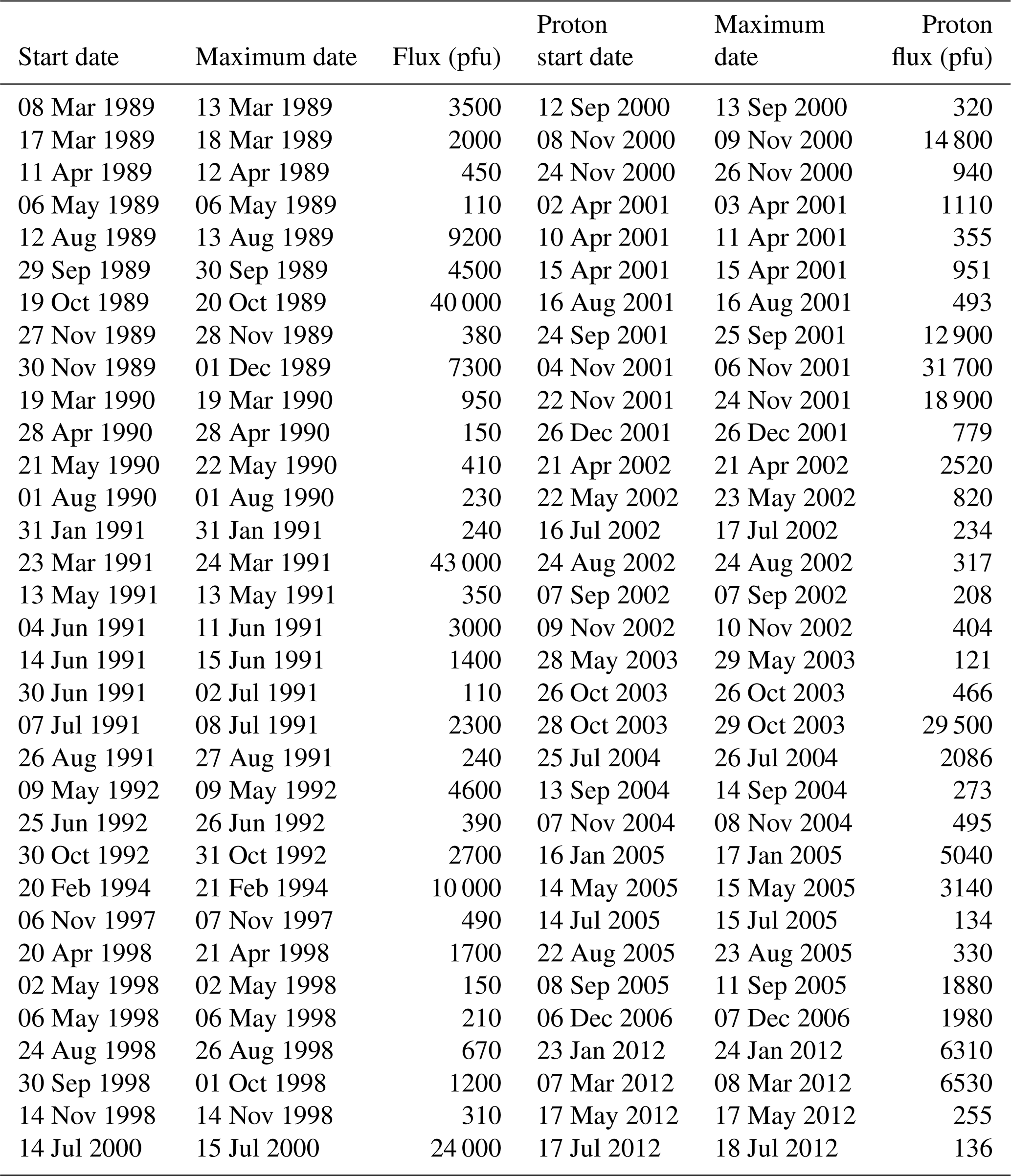
For our statistical analysis, SPEs were selected using proton flux data from satellite-based GOES observations (available from https://www.ngdc.noaa.gov/stp/satellite/goes/index.html, last access: 9 July 2020). An event was selected if the peak proton flux exceeded 100 particle flux units (pfu), with pfu defined as the 5 min average flux in units of particles cm⁻² s⁻¹ sr⁻¹ for protons with energy larger than 10 MeV. To avoid obscuring the signal in composite means by introducing duplicates of major events in days preceding the zero epoch date, any event following a larger event onset within 7 d was excluded from the analysis. In total, 11 such events were removed. Following these criteria, 66 events given in Table A1 were identified in the simulation period. The seasonal distribution of the selected SPEs is shown in Fig. 1. As SPEs are sporadic, the distribution is somewhat uneven, with the Northern Hemisphere winter months (December–February) underrepresented. Of the 8 largest SPEs (above 10 000 pfu) in the analysis, five occurred in October or November, compared to only one each in March, July and September.

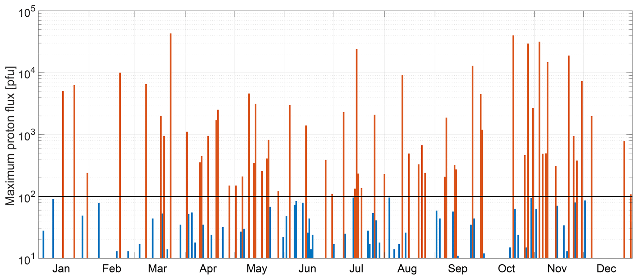
Figure 1Maximum proton flux of solar proton events used in the analysis as a function of the day of the year of the SPE onset. Events with maximum flux over threshold value (100 pfu) are shown as red bars and smaller events as blue bars.

Download

Table 1Definitions used in the text for the SD-WACCM and WACCM-D simulations.

Download Print Version | Download XLSX

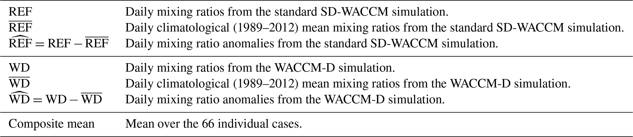
For each of the 66 events, zero epoch day (D₀) was defined as the first day when the proton flux exceeded 10 pfu. A 90 d epoch period around the zero epoch ([D₀−29, D₀+60]) was selected from the daily mean time series for the following constituents: O₃, HO_x (OH + HO₂), Cl_x (Cl + ClO), HNO₃, NO_x (NO + NO₂) and H₂O. Definitions of abbreviations used in the following text for the statistical quantities from REF and WD simulations are shown in Table 1.

To assess the anomalies $\widehat{\mathrm{REF}}$ and $\widehat{\mathrm{WD}}$ associated with the SPEs, daily climatological mean mixing ratios $\stackrel{\mathrm{‾}}{\mathrm{REF}}$ and $\stackrel{\mathrm{‾}}{\mathrm{WD}}$ were deducted from respective epoch mixing ratios REF and WD. Figure 2 shows the composite means of $\stackrel{\mathrm{‾}}{\mathrm{WD}}$ for the northern polar cap (60–90^∘ N, area-weighted). Note that due to the seasonal distribution of the events some seasonal signals remain visible in the composite means, e.g., a slight increase in mesospheric O₃ during the 90 d epoch period. It can also be seen that for some constituents, especially HNO₃, mixing ratio enhancements following the events are large enough to visibly affect the daily climatology.

Figure 2Area-weighted northern polar cap (latitude $>{\mathrm{60}}^{\circ }$ N) average of composite mean of $\stackrel{\mathrm{‾}}{\mathrm{WD}}$ for O₃, HO_x, Cl_x, HNO₃, NO_x and H₂O. The x axis shows the number of days before and after the event (day 0, solid black line) and the y axis pressure levels in the model (hPa, a, d) and approximate altitude (km, c, f).

Download

For each constituent, we calculate the composite mean of difference μ_d between the epoch time series and the corresponding climatological time series

where r is the relevant mixing ratio epoch time series REF or WD, c is the epoch time series from daily climatology $\stackrel{\mathrm{‾}}{\mathrm{REF}}$ or $\stackrel{\mathrm{‾}}{\mathrm{WD}}$, and d is the number of days before and after zero epoch $D_{{\mathrm{0}}_i}$. Subtracting the climatological values from the epoch time series helps to separate the SPE signal from the seasonal signals which can arise from the uneven monthly distribution of the SPEs (see Fig. 1). Variance of the composite means was approximated by bootstrapping, i.e., by re-sampling the random selection of dates 1000 times with replacement, with N=66 for each sample. Bootstrapping was chosen for variance estimation due to its independence from the shape of the distribution; i.e., it does not require a normal distribution. The standard deviation of the variance was then used to identify robust responses, i.e., SPE-driven changes that are clearly larger than the normal variability.

The SPE-driven anomalies are expected to occur following the SPE onset (zero epoch). However, in Sect. 3 we will show that the results sometimes have also anomalies that extend over the full epoch period. These anomalies are in most cases related to solar cycle variability, due to the SPE sampling over-representing the solar cycle maximum years when compared to climatology. Composite mean SPE ionization for the analyzed epochs is shown in Fig. 3. Daily composite mean peak ionization is 891 ion pairs cm⁻³ s⁻¹, which is roughly similar in magnitude to peak ionization associated with January 2005 SPE. The largest individual events in the time series feature peak ionizations about 10 times higher, for example peak ionization of 8534 ion pairs cm⁻³ s⁻¹ for the “Halloween” SPE. In addition to the main ionization peak within ca. 5 d following the onset of the SPE, secondary ionization peaks are evident in the epoch mean, due to closely separated SPEs. While these secondary peaks are much weaker (by roughly an order of magnitude) than the main peak, they can still cause noticeable anomalies in some of the analyzed constituents.

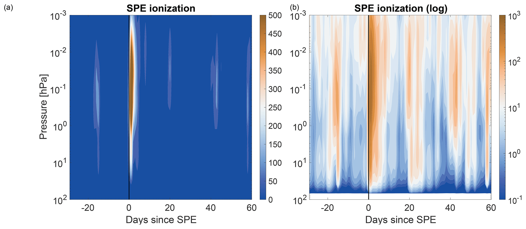
Figure 3Composite mean of epoch time series of SPE ionization rates in linear (a) and logarithmic (b) color scale. The x axis shows the number of days before and after the event (day 0, solid black line) and the y axis pressure levels in the model.

Download

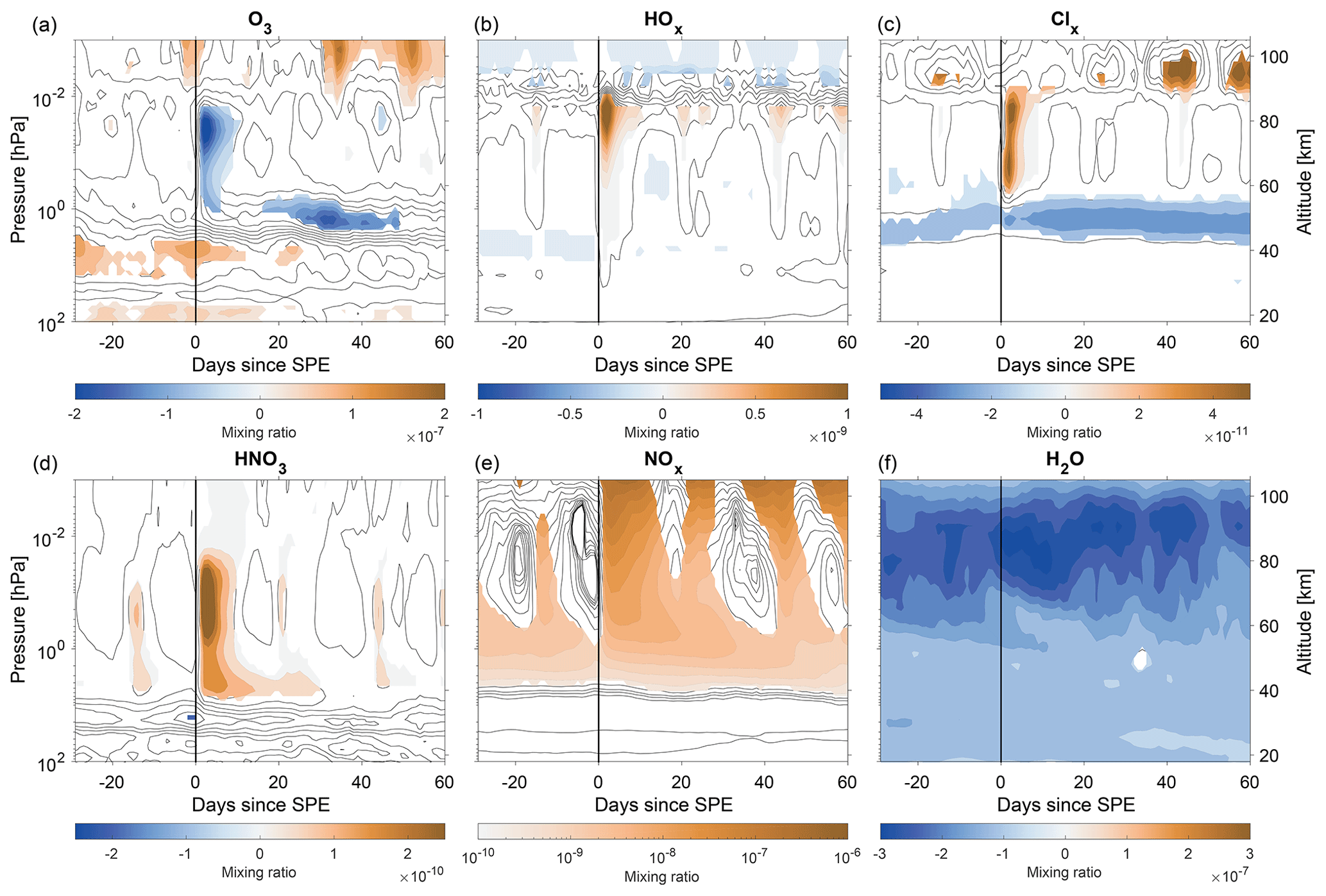
Figure 4Area-weighted northern polar cap averages (latitude $>{\mathrm{60}}^{\circ }$ N) of composite means of $\widehat{\mathrm{WD}}$ for O₃, HO_x, Cl_x, HNO₃, NO_x and H₂O. The x axis shows the number of days before and after the event (day 0, solid black line) and the y axis pressure levels in the model (hPa, a, d) and approximate altitude (km, c, f). Note that the color scale for NO_x panel is logarithmic, and all contours shown in that panel indicate positive difference.

Download

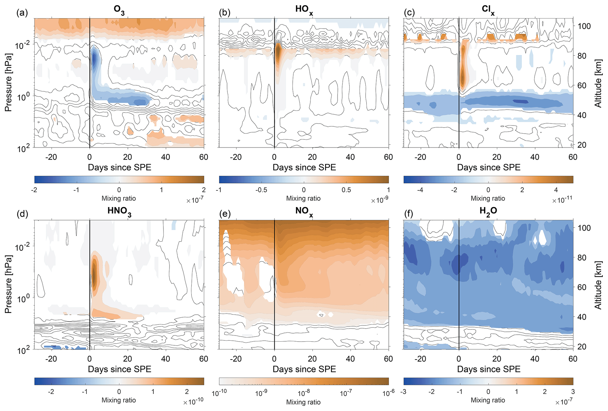
Figure 5Area-weighted southern polar cap averages (latitude $>{\mathrm{60}}^{\circ }$ S) of composite means of $\widehat{\mathrm{WD}}$ for O₃, HO_x, Cl_x, HNO₃, NO_x and H₂O. The x axis shows the number of days before and after the event (day 0, solid black line) and the y axis pressure levels in the model (hPa, a, d) and approximate altitude (km, c, f). Note that the color scale for NO_x panel is logarithmic, and all contours shown in that panel indicate positive difference.

Download

In order to evaluate the contribution of the improved ion chemistry of WACCM-D, the same epoch analysis was made for both the REF and the WD simulations. The anomalies from the WACCM-D simulation ($\widehat{\mathrm{WD}}$) were then compared to anomalies from the standard WACCM ($\widehat{\mathrm{REF}}$) (Figs. 4 and 5). We considered the difference of composite means of differences in mixing ratio between the two simulations for the full altitude range (Figs. 6 and 7) as well as comparison of the SPE response at pressure levels chosen for maximum difference between two simulations (Figs. 8 and 9).

3.1 Statistical response from WACCM-D

Figures 4 (Northern Hemisphere, NH) and 5 (Southern Hemisphere, SH) show the mean anomaly of the super-imposed epochs for O₃, HO_x, Cl_x, HNO₃, NO_x and H₂O. Statistically robust anomalies, i.e., those larger than 2 times the standard deviation of the bootstrap variance, are shown in color and discussed below.

Several constituents show the most pronounced anomaly immediately following the event onset (zero epoch), which in the figures is marked with a black vertical line. For some constituents, most notably H₂O and Cl_x, persistent anomalies extending throughout the epoch period are seen as well. These anomalies can be considered to represent the solar cycle signal because the distribution of SPEs concentrates on the years around the solar maximum. Some anomalies are clearly affected by the response to closely separated SPEs, i.e., when the separation is smaller than 60 d. These are most notable in NO_x and HNO₃ in NH around days −15, +22 and +45 with respect to zero epoch, corresponding to the secondary peaks of SPE ionization (see Fig. 3).

Ozone (Figs. 4 and 5, panel a) decreases between 1 and 0.01 hPa immediately following the SPE, lasting about 5–10 d. This is caused by catalytic destruction from enhanced HO_x. Ozone loss also takes place around 1 hPa, driven by NO_x and Cl_x. The depletion around 1 hPa lasts much longer, driven by the NO_x increase, with maximum ozone decrease seen about 30 d after the event onset. In contrast, an increase in ozone is seen throughout the period near the secondary ozone maximum above 0.01 hPa, more robustly in the Southern Hemisphere. This increase is linked to enhanced atomic oxygen production by O₂ photolysis in solar maximum conditions (see also Marsh et al., 2007). In the stratosphere below 5 hPa the ozone response is not consistently robust. However, an intermittent increase, likely caused by solar cycle effects, is seen throughout the epoch period in this region. Thus the decrease in the total ozone column, as reported by Denton et al. (2018), is not seen in our analysis. It should be noted that the highest energy protons (E>300 MeV), which can directly impact the lower stratosphere, are not included in the particle forcing used in our simulations. However, it is not clear whether inclusion of these protons would change the response because their fluxes should be too low to cause a significant extra response (Jackman et al., 2011).

A strong, short-lived increase in HO_x is seen below 0.01 hPa (Figs. 4 and 5, panel b) immediately following the SPE, reaching down to the 10 hPa level, with the strongest and the most robust response in the mesosphere. Due to the short chemical lifetime of HO_x, there is no longer-term anomaly beyond 10 d from the SPE onset. The later peaks just below 0.01 hPa are caused by SPEs occurring within 60 d of zero epoch of analyzed SPE. Above 0.01 hPa, a small negative anomaly is present throughout the period, related to solar maximum through less water vapor in the region and lowering of the HO_x peak altitude. The persistent positive anomaly at just below 0.01 hPa, seen in the SH, is consistent with lowering of the HO_x peak altitude. Factors affecting HO_x peak altitude during solar maxima are the decrease in H₂O and the increase in Lyman-α photolysis, balancing at the level of mesopause.

Cl_x mixing ratios (Figs. 4 and 5, panel c) are enhanced between 1 and 0.01 hPa, these SPE-driven increases last up to about a week. Below 1 hPa, at the altitude of Cl_x mixing ratio maximum, Cl_x is a reduced. This decrease is roughly consistent and continuous throughout the epoch period and so is likely, at least in part, connected to the solar cycle rather than individual events. However, the magnitude of the negative anomaly increases following the onset of the SPE, with maximum value in the SH reached after 30 d. A short-lived decrease in the NH polar upper stratosphere ClO during the January 2005 SPE has previously been reported both in satellite observations and models (Damiani et al., 2012; Andersson et al., 2016). In the short term decrease is likely caused by conversion of ClO to HOCl in the presence of enhanced HO₂, while in the longer term, the decrease is probably connected to the descent of NO_x and subsequent formation of ClONO₂. Here we look at the polar average, but it should be noted that in the presence of SPE-generated HO_x, the response of Cl_x in the polar atmosphere depends strongly on the sunlight conditions and varies across latitudes and altitudes (Funke et al., 2011). For example, in the polar night stratosphere ClO is converted to HOCl in reaction with HO₂, while in the daytime HOCl is converted to ClO by OH.

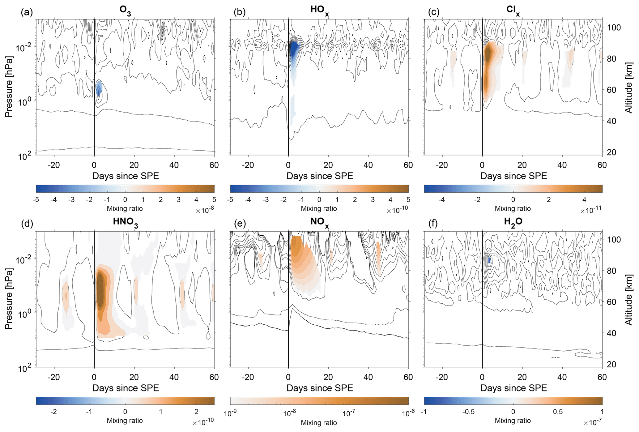
Figure 6Area-weighted northern polar cap averages (latitude $>{\mathrm{60}}^{\circ }$ N) of composite means of $\widehat{\mathrm{WD}}$ – $\widehat{\mathrm{REF}}$ (see Fig. 4). The x axis shows the number of days before and after the event (day 0, solid black line) and the y axis pressure levels in the model (hPa, a, d) and approximate altitude (km, c, f). Note that the color scale for NO_x panel is logarithmic, and all contours shown in that panel indicate positive difference.

Download

A large increase in HNO₃ (Figs. 4 and 5, panel d) is seen up to 10 d after the SPE onset, with a maximum between 1 and 0.01 hPa. The absence of a longer-term effect is due to the fast photodissociation of HNO₃ in sunlit conditions. Similar to HO_x, the later peaks around days 20 and 45 in the NH are caused by nearly coincident SPEs. A longer-term enhancement persists for 20–30 d after SPEs below 1 hPa. The anomalies are weaker in the SH than in the NH, due to the strongest SPEs mostly occurring during NH winter (see Fig. 1) when there is less solar radiation and HNO₃ photodissociation.

SPE-driven enhancements of NO_x (Figs. 4 and 5, panel e) reach down to 1 hPa level and below. These enhancements start to diminish after about 10 d, but robust longer-term enhancements can be seen for several weeks afterwards. This is especially clear at lower altitudes (around 1 hPa), where transport from above contributes to persistence of enhancements. The response is different in the Northern and Southern Hemispheres due to the seasonal distribution of the events. In the NH, several strong, closely separated winter-time events show up as recurring anomalies, which are then transported to lower altitudes. The SH response is less variable, with small but robust enhancements seen through the two months following the SPE onset. In addition to the SPE-driven anomaly, there is a persistent, underlying anomaly seen above about 10 hPa from enhanced NO_x production in the lower thermosphere by solar EUV and EPP during solar maximum times (see also Marsh et al., 2007).

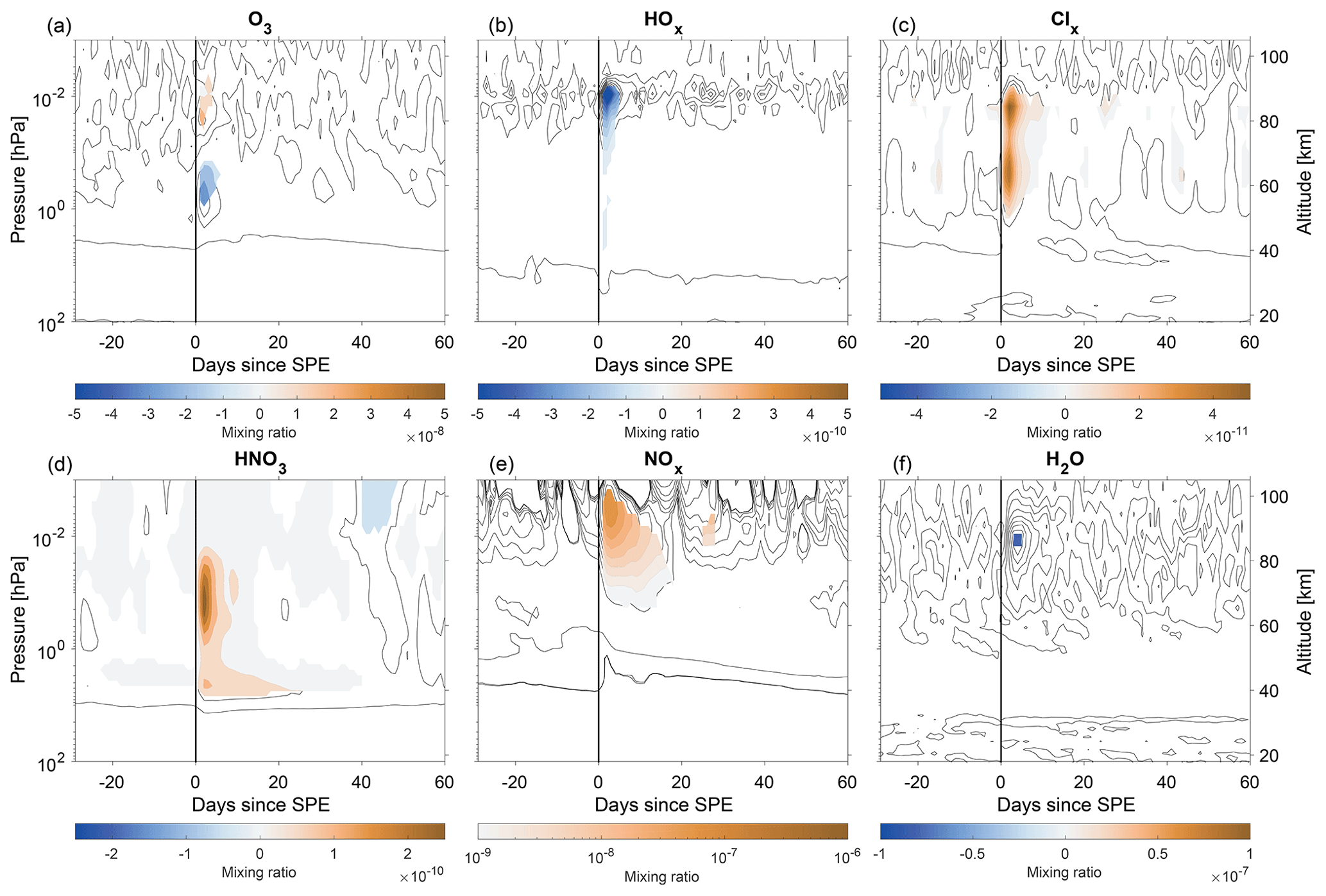
Figure 7Area-weighted southern polar cap averages (latitude $>{\mathrm{60}}^{\circ }$ S) of composite means of $\widehat{\mathrm{WD}}$ – $\widehat{\mathrm{REF}}$ (see Fig. 5). The x axis shows the number of days before and after the event (day 0, solid black line) and the y axis pressure levels in the model (hPa, a, d) and approximate altitude (km, c, f). Note that the color scale for NO_x panel is logarithmic, and all contours shown in that panel indicate positive difference.

Download

During an SPE, H₂O would be expected to decrease when it is converted to HO_x in ionic reactions. In our analysis, H₂O (Figs. 4 and 5, panel f) shows a consistent and statistically robust negative anomaly throughout the period analyzed, except in the SH lower stratosphere. There is some indication of a stronger anomaly following the SPEs above 0.1 hPa, i.e., at altitudes where HO_x increases. But in general the anomaly is mostly related to the solar cycle through the increased Lyman-α photodissociation during solar maximum decreasing H₂O in the mesosphere–lower thermosphere (see also Schmidt et al., 2006; Marsh et al., 2007).

3.2 Effects of D-region ion chemistry

Figures 6 and 7 show the difference between epoch responses in the NH and SH, respectively, from WACCM-D and the standard WACCM. As the specified dynamics of the two simulations are identical, differences seen in these figures arise from the addition of the D-region ion chemistry. Note that the robustness threshold for these figures is set to 1 standard deviation rather than the 2 standard deviations used in Figs. 4 and 5. The differences shown in figures for constituents other than O₃ and H₂O also satisfy the threshold of 2 standard deviations. The effects on O₃ and H₂O, however, do not reach the threshold of 2 standard deviations. Further, Figs. 8 and 9 show line plots of epoch response from both WACCM-D ($\widehat{\mathrm{WD}}$) and standard WACCM ($\widehat{\mathrm{REF}}$) at pressure levels corresponding to maximum significant difference in Figs. 6 and 7.

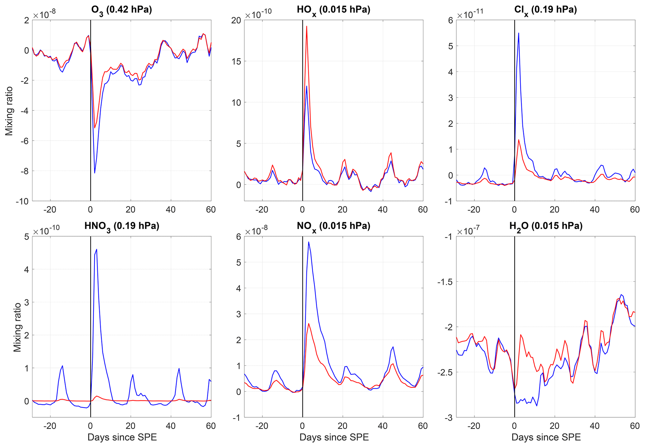
Figure 8Composite mean $\widehat{\mathrm{WD}}$ (blue) and $\widehat{\mathrm{REF}}$ (red) for the northern polar cap (area-weighted, latitude $>{\mathrm{60}}^{\circ }$ N) at selected pressure bands (three pressure levels, pressure of the center of the band shown in panel title). The x axis shows the number of days before and after the event (day 0, solid black line).

Download

Ozone (Figs. 6 and 7, panel a) depletion is larger in WACCM-D for about 5 d after the onset at around 0.5–1 hPa. This effect is very similar in both hemispheres. Both the duration and altitude range of this extra ozone loss clearly correspond to enhanced Cl_x, while there is no clear connection to NO_x or HO_x differences. Less ozone depletion takes place in WACCM-D around the 0.01 hPa level, connected to the clearly lower HOx enhancement in WACCM-D. An anomaly of similar magnitude is observed in both hemispheres, although it is only robust in SH. The reduced HO_x response in WACCM-D is a result of the lower water vapor amount, and thus lower HO_x production, than what is assumed when HO_x production is parameterized (Andersson et al., 2016).

Cl_x is enhanced in both hemispheres above 1 hPa in WACCM-D, while there is only a relatively weak increase in the standard WACCM. The reasons for the enhancement are the ion reactions included in WACCM-D that convert more HCl to active chlorine species Cl and ClO (Winkler et al., 2009) than the neutral gas-phase reactions which are included in both standard WACCM and WACCM-D. Enhancements relating to secondary ionization peaks can also be seen, most clearly around day 40. The negative anomaly of Cl_x below 1 hPa seen in Figs. 4 and 5 is not present here, again implying that this anomaly is not predominantly due to ion chemistry.

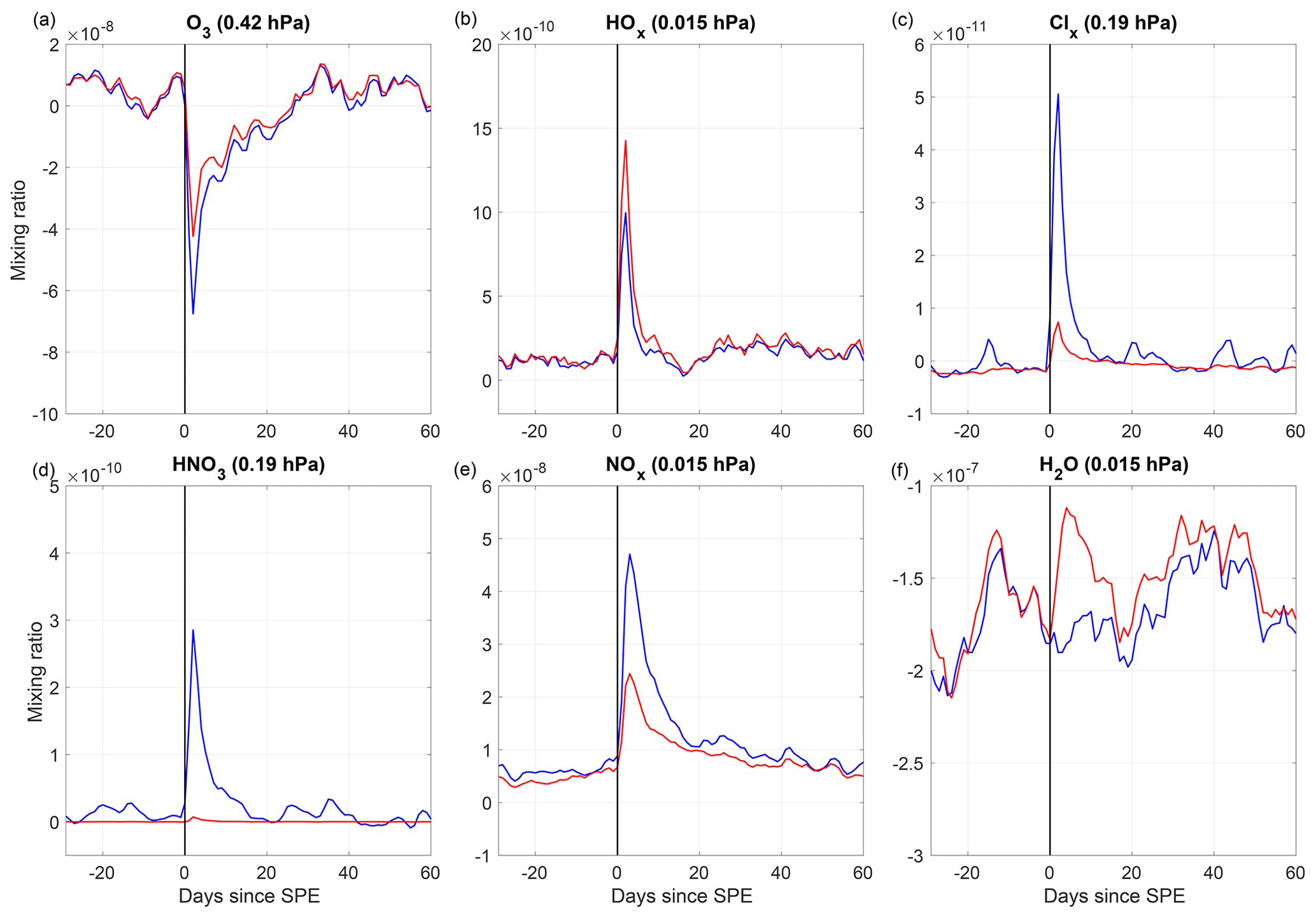
Figure 9Composite mean $\widehat{\mathrm{WD}}$ (blue) and $\widehat{\mathrm{REF}}$ (red) for the southern polar cap (area-weighted, latitude $>{\mathrm{60}}^{\circ }$ S) at selected pressure bands (three pressure levels, pressure of the center of the band shown in panel title). The x axis shows the number of days before and after the event (day 0, solid black line).

Download

The HNO₃ enhancement is clear and strong in WACCM-D, as ion chemistry produces it from other NO_y species. Standard WACCM, like other models using an EPP lookup table parameterization, is known to underestimate the HNO₃ mixing ratios when compared to observations (Jackman et al., 2008; Funke et al., 2011; Andersson et al., 2016). A discrepancy between WACCM-D and standard WACCM HNO₃ enhancements is clearly seen in Figs. 8 and 9. Due to the dramatic increase in HNO₃ following SPEs, peaks from other, close-by events are also clearly seen in Fig. 8.

In the mesosphere, the NO_x enhancement is much larger in WACCM-D than in standard WACCM. Below 0.1 hPa there are some signs of an increase in transported NO_x, although this effect is not statistically robust. Increased NO_x is consistent between the hemispheres. Andersson et al. (2016) attribute the increased NO_x to enhanced production above 80 km (ca. 0.01 hPa), mostly due to the reaction ${\mathrm{O}}_{\mathrm{2}}^{+}$ + N₂ → ${\mathrm{NO}}^{+}+\mathrm{NO}$, and consequent transport to lower altitudes.

Differences in H₂O anomalies (Figs. 6–9, panel f) between WACCM-D and the standard WACCM are seen above 1.0 hPa but they are almost entirely overcome by the variance, which indicates that negative anomalies in Figs. 4 and 5 are not primarily connected to ion chemistry reactions but are a solar cycle signal. However, a short-lived negative difference, robust to a 1σ level, can be seen at 0.01 hPa immediately following the onset of SPE, even though the co-located HO_x production in WACCM-D is smaller. This negative difference is more clearly seen in Figs. 8 and 9, where we see that mesospheric H₂O anomalies are very consistent between the simulations, except within 10–15 d following the onset of SPE, where the WACCM-D negative anomalies are larger.

Figure 10$\widehat{\mathrm{WD}}$ of individual SPEs at 0.05 hPa pressure level, sorted by the increasing SPE magnitude for the northern (a, c, e) and southern (b, d, f) polar caps. Dashed lines represent the 100 (bottom line) and 1000 (top line) pfu limits.

Download

3.3 Effect from individual events

The SPE effects are dependent on the background atmosphere and season of the year. Here we discuss this by looking at the effects of individual events at selected altitudes. This is also an additional check on the robustness of our analysis.

Figure 10 shows the individual time series of differences of epochs from the climatology around 0.05 hPa pressure level (calculated as the mean of three pressure levels centered at 0.04 hPa). SPEs used in this figure are screened for closely separated events, i.e., events which are followed by a larger event within 7 d are not shown. Individual events are sorted from top to bottom by the maximum observed proton flux, with strongest events on top of the figure. Dashed horizontal lines show the cut-offs for 1000 pfu (top line) and 100 pfu (bottom line) SPEs.

As expected, the largest SPEs cause a stronger response in O₃, HO_x and NO_x. The response to events is more pronounced in the NH due to the seasonal distribution of SPEs; i.e., there are more events in NH winter. This is especially apparent for NO_x, as its lifetime is heavily influenced by the amount of sunlight available. On visual inspection, the response is dominated by the largest SPEs, with anomalies following the onset of SPEs being visually indistinguishable for the weakest events. Below the 100 pfu threshold, any anomalies following the event onset are dominated by larger events occurring within the analysis period, rather than by the analyzed event itself. Thus, the decision to only analyze larger events seems reasonable because the events smaller than 100 pfu would only add a substantial amount of noise to the analysis.