2.1 Age spectrum

The full information on the distribution of transport times is given by the actual age spectrum. The age spectrum is the distribution of transport times of trace gas concentrations to the location of interest x. Thus, it is equated to the Green's function (G) that describes the propagation of the tracer concentration χ₀ from the reference location to the observed location. This can be expressed with the following equation.

in which case t denotes the transit time. The first moment of the age spectrum is the mean AoA Γ. This is written as

Consequently, the second moment of G(t) is defined as

A well-known approximation for G(t) is given by an inverse Gaussian by Hall and Plumb (1994), which uses the first and second moment Γ and Δ

This equation was obtained from a one-dimensional diffusion analogue. Usually, Δ² is parameterized relative to Γ as ${\mathrm{\Delta }}^{\mathrm{2}}=C_{\mathrm{1}}\cdot \mathrm{\Gamma }$. Figure 1 illustrates the effect of different values of $\frac{{\mathrm{\Delta }}^{\mathrm{2}}}{\mathrm{\Gamma }}$ on Eq. (4). In a conceptual sense, Δ² can be expressed relative to Γ as the longer air has been traveling (i.e. larger Γ), the more spread out the age spectrum will be (i.e. larger Δ²). The specific value of $\frac{{\mathrm{\Delta }}^{\mathrm{2}}}{\mathrm{\Gamma }}$ describes how strong this spreading out is (Waugh and Hall, 2002).

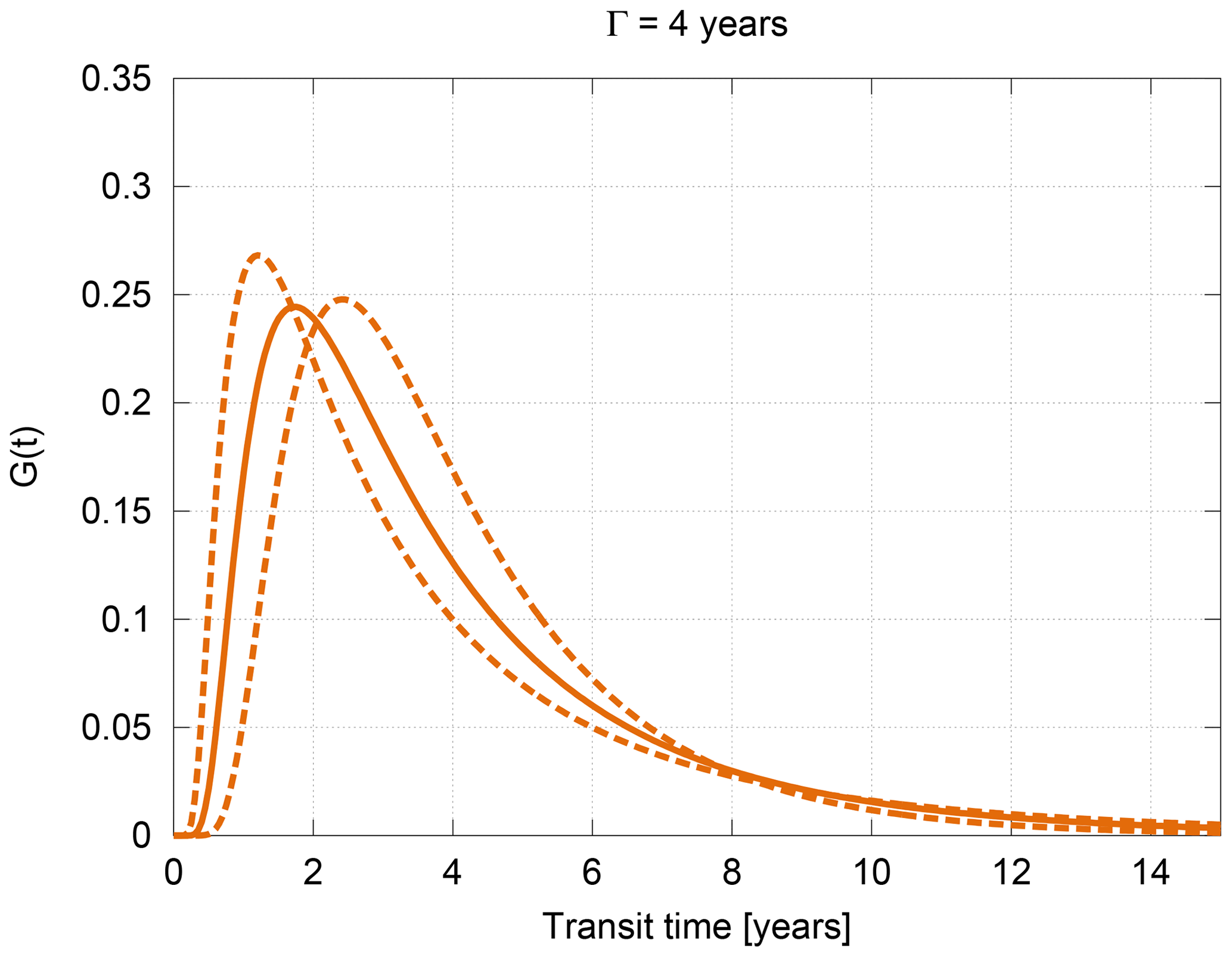
Figure 1Sketch to illustrate the ratio of moments. The resulting age spectra from an inverse Gaussian with mean 4 years for values of $\frac{{\mathrm{\Delta }}^{\mathrm{2}}}{\mathrm{\Gamma }}$ 0.7, 1.25 and 2.0 years.

Download

More detailed approaches considered two-peak age spectra (Andrews et al., 2001). However, in models the exact age spectrum can be obtained. If we consider Eq. (1), Green's function can be obtained from a delta peak in tracer concentration. In the case of a non-stationary atmosphere, i.e. one with seasons, a set of inert tracer pulses at a reference surface is required. This method was already described and implemented for different models in e.g. Li et al. (2012) and Ploeger and Birner (2016).

2.2 Linear tracers

A well-established way to derive Γ in models is from a linearly increasing inert tracer. In this case, the mean age at a point x is equal to the time lag τ of the tracer concentration χ relative to the concentration χ₀ at a selected reference area, which can be written as

2.3 Non-linear tracers

2.3.1 Quadratic fit to the reference time series

In the real world, no perfectly linear increasing inert tracer is available. Often, SF₆ is used as a proxy for such a tracer. As the SF₆ emissions increase non-linearly, a common approach to derive mean AoA is a second-order approximation that considers the slope of the reference time series. The general concept of the derivation is described in Volk et al. (1997). Engel et al. (2009, 2017) apply it as an iterative procedure to optimize the length of the fit interval to the reference time series. First, the second-order fit is performed on the reference time series for a set fit interval, e.g. 15 years. This yields the polynomial coefficients a, b and c. The fit performed can be expressed either relative to the nominal time axis $\stackrel{\mathrm{̃}}{t}$ ranging from 1960 to 2011 and the reference time t₀ or by the transit time t (note the change in sign):

$$\begin{array}{}\text{(6)}& {\mathit{\chi }}_{\mathrm{0}}\left(\stackrel{\mathrm{̃}}{t}\right)=a+b\left(\stackrel{\mathrm{̃}}{t}-t_{\mathrm{0}}\right)+c{\left(\stackrel{\mathrm{̃}}{t}-t_{\mathrm{0}}\right)}^{\mathrm{2}}=a-bt+t^{\mathrm{2}}.\end{array}$$

Secondly, a first guess for the mean age is calculated using the coefficients applying the equation (Volk et al., 1997)

$$\begin{array}{}\text{(7)}& \mathrm{\Gamma }={\displaystyle \frac{b}{\mathrm{2}c}}-C_{\mathrm{1}}\pm \sqrt{{\left({\displaystyle \frac{b}{\mathrm{2}c}}-C_{\mathrm{1}}\right)}^{\mathrm{2}}+{\mathit{\tau }}^{\mathrm{2}}-{\displaystyle \frac{b}{c}}\cdot \mathit{\tau }}.\end{array}$$

Again, Δ is the width of the age spectrum and C₁ is the ratio of first and second moments of the age spectrum omitting a factor of 2; i.e. $C_{\mathrm{1}}=\frac{{\mathrm{\Delta }}^{\mathrm{2}}}{\mathrm{\Gamma }}$. C₁ parameterizes the width of the spectrum relative to its mean. Again, τ is the lag time between the concentrations χ and χ₀. To be consistent with Engel et al. (2017), the lag time is determined by approximating the reference time series by a second-order polynomial. In the third step, a fit interval t_fit is determined, which considers a given fraction of input (F) of the age spectrum, e.g. 98 %. This can be written as

$$\begin{array}{}\text{(8)}& \underset{\mathrm{0}}{\overset{t_{\mathrm{fit}}}{\int }}G\left(t^{\prime }\right)\mathrm{d}{t}^{\prime }\stackrel{!}{=}F.\end{array}$$

More schematically, the fraction of input is illustrated in Fig. 2. Considering a given fraction F of the area enclosed by G(t) gives a transit time that corresponds to this fraction, and this transit time is then used as a backward fit interval to perform the fit on the reference time series. Thus, the larger the fraction of input F, the longer the fit interval. The age spectrum G(t) assumed in this step is the inverse Gaussian from Eq. (4). This equation uses the previous mean age value and the parameterization for the width. In the last step the value for the fit interval is used to determine once more the polynomial coefficients and recalculate the mean age value according to Eq. (7).

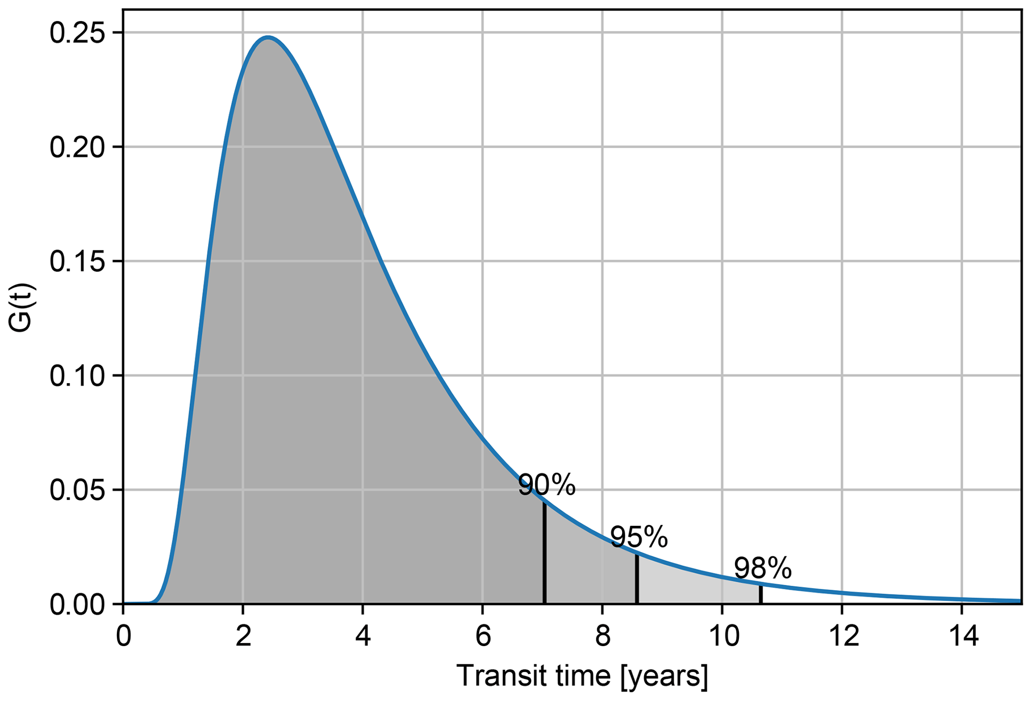
Figure 2The resulting fit intervals for the fraction of input F=90 %, 95 % and 98 % are sketched. G(t) is assumed from an inverse Gaussian for Γ=4 years and ${\mathrm{\Delta }}^{\mathrm{2}}=\mathrm{0.7}\cdot \mathrm{\Gamma }$.

Download

Summing up, to perform this procedure one needs to choose the reference point, the fraction of the considered input and the ratio of the moments. Our aim is to systematically test the sensitivity of the derived mean AoA and AoA trends to those parameters.

2.4 EMAC simulations

In the present study, we use the results of two simulations of the chemistry-climate model EMAC (ECHAM/MESSy Atmospheric Chemistry, Jöckel et al., 2010), which are both in a T42 horizontal (2.8×2.8^∘) resolution with 90 layers in the vertical and explicitly resolved middle atmosphere dynamics (T42L90MA). In this setup, the uppermost model layer is centered at around 0.01 hPa and the vertical resolution in the upper troposphere lower stratosphere region (UTLS) is 500–600 m. MESSy (Modular Earth Submodel System) provides an infrastructure with generalized interfaces for standardized coupling of Earth system model (ESM) components (dynamical cores, physical parameterizations, chemistry packages, diagnostics, etc.). The dynamical core of EMAC is the European Center Hamburg general circulation model (ECHAM5, Roeckner et al., 2006).

The first simulation is a free-running transient hindcast simulation using EMACv2.51 with full interactive chemistry stretching from 1960 to 2011. This simulation was performed within the ESCiMo project (Earth System Chemistry integrated Modeling, Jöckel et al., 2016) and is referred to as RC1-base-07. The setup of this simulation follows the REF-C1 scenario as defined by the Chemistry-Climate Model Initiative (CCMI, Eyring et al., 2013). Details on the setup and an evaluation of this chemistry-climate simulation can be found in Jöckel et al. (2016) and in Morgenstern et al. (2017). The simulation had 10 years of spin-up, i.e. 1950–1959. This means that for the earliest AoA values calculated for 1975 the respective fit back along the reference time series does not stretch into the spin-up period. Previous tests showed that this spin-up length is sufficient to not affect mean AoA.

The second simulation, termed tranPul, is an EMACv2.53.0 run which is designed to resemble the RC1-base-07 simulation as closely as possible, for cost efficiency reasons however, without using interactive chemistry. This means that only the EMAC modules for dynamics, physics and diagnostics were used, namely AEROPT, CLOUD, CLOUDOPT, CONVECT, CVTRANS, E5VDIFF, ORBIT, OROGW, PTRAC, RAD, SURFACE, TNUDGE, TROPOP, and VAXTRA. For details on these submodels, refer to Jöckel et al. (2005, 2010, 2016). In that simulation, we transiently prescribed the monthly mean fields of the main greenhouse gases CO₂, CH₄, N₂O and O₃ from the RC1-base-07 simulation as zonal mean, monthly mean fields. As both simulations do not include a coupled ocean, SSTs and SICs have been prescribed following the HadISST global data set provided by the UK Met Office Hadley Centre (available via http://www.metoffice.gov.uk/hadobs/hadisst/ – last access: 29 June 2020; Rayner et al., 2003). Although in the L90 setup of EMAC the quasi-biennial oscillation (QBO) is internally generated (Giorgetta et al., 2002), the zonal winds near the Equator were slightly nudged in the simulations to get the correct phasing of the observed QBO. Moreover, atmospheric aerosol (including volcanic aerosol) has been prescribed to take into account the interactions with radiation (in both simulations) and with heterogeneous chemistry (in the RC1-base-07 simulation). Again, 10 years of spin-up were considered.

The RC1-base-07 simulation is used to study the methods that are used to derive AoA from non-linear tracers, such as SF₆. As our focus is to quantitatively assess the uncertainties of the mean AoA derivation, the SF6 tracers considered in these simulations do not include mesospheric sinks. The SF₆ time series prescribed in the simulation follows the RCP6.0 scenario (Eyring et al., 2013). Its global mean is shown in Fig. 3 as it is prescribed in the simulations to emulate emissions. The SF₆ time series as applied with the calculations from measurements is also displayed (see Levin et al., 2010; Maiss and Levin, 1994). From 1978 on, the time series is well constrained by NOAA measurements at Cape Grim. Before that, SF₆ is estimated from emissions. Prior to 1961, the data were linearly extrapolated. Both SF₆ time series differ slightly, as can be seen from Fig. 3. However, as explained in detail in Sect. 3.2, this does not impact our method evaluation.

Figure 3Globally averaged SF₆ time series on the ground as used in the RC1-base-07 simulation (blue) and as used with the observation calculations (red).

Download

In the tranPul simulation, periodical pulses of an inert tracer were released at the surface in the range between 20^∘ S and 20^∘ N. This means that every 3 months, the lower boundary conditions of that tracer are set to 1 for 1 month at the tropical surface. After 9.5 years, the tracers are set to zero and started again to avoid large computational expenses. This operation is performed with the specifically designed MESSy submodule TPULSE. A similar EMAC setup was already applied in Hauck et al. (2019). The pulses allow the derivation of time-evolving age spectra in EMAC as described for CLaMS (Chemical Lagrangian Model of the Stratosphere) in Ploeger and Birner (2016).

3.1 Age spectra

It is straightforward to derive mean AoA from linearly increasing tracers in models, as described in Sect. 2.2. To give an example of mean AoA in EMAC, Fig. 4 shows mean AoA derived from the idealized linear increasing tracer for July 2001–2010 from the RC1-base-07 simulation. Since the derivation of mean AoA from measurements requires an assumption about the AoA spectrum, we derived spectra for EMAC in a transient simulation. The implementation was such that tracer pulses were released every 3 months and kept running for 9.5 years, which is due to the technical realization. Figure 5 shows the seasonal evolution of the modelled spectra at 59^∘ N and 106 hPa. This is close to 400 K and 60^∘ N potential temperature, as in Fig. 5 in the study by Ploeger and Birner (2016). The MAM, JJA and SON spectra show a similar propagation to Ploeger and Birner (2016). DJF rather shows one major peak instead of two as in Ploeger and Birner (2016). Our coarse resolution of the spectra along the transit time axis of 3 months could be the reason for this, since the actual maxima of the age spectrum may fall in between a 3-month period such that they are not visible. For comparison, the spectrum calculated from the Hall and Plumb parameterization (see Eq. 4) is shown, using the values from the annual mean spectrum, that is, a mean age value of 1.6 years (vertical line) and a ratio of moments of 1.8 years. For the chosen parameters, the modal age of the theoretical Hall and Plumb spectrum is lower than for the actual spectrum and the tail is broader. However, how well the modal age compares depends strongly on the applied ratio of moments.

Figure 4Mean AoA derived from the idealized tracer from the RC1-base-07 ESCiMo simulation. July mean for the years 2001–2010.

Download

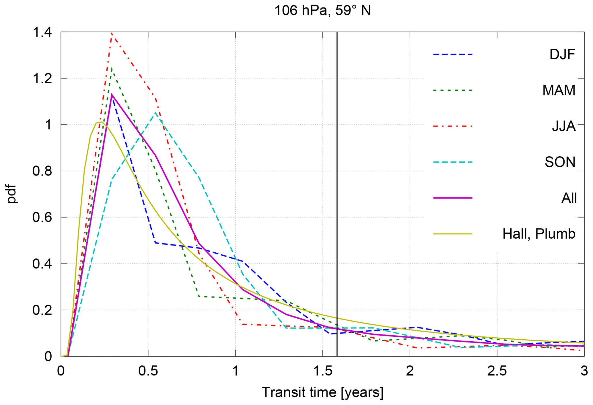
Figure 5Age spectra at 59^∘ N and 106 hPa from the tranPul simulation. The dashed lines are the seasonal mean spectra. The pink solid line is the annual mean age spectrum. The solid yellow line is the spectrum calculated from the Hall and Plumb parameterization using the values from the integration of the annual mean spectrum, that is, a mean age value of 1.6 years (vertical line) and a ratio of moments of 1.8 years (Eqs. 2 and 3).

Download

The ratio of moments calculated directly from the spectra as shown in Fig. 6 (left) are small (considering the length of the spectra of 9.5 years), considering values of 0.7 to 1.25 years are proposed for age calculations in Hall and Plumb (1994). Following Ploeger and Birner (2016), the spectra were extended to 50 years using an exponential fit on the second half of the spectrum, i.e. transit times above 5 years. The ratio of moments in that case (Fig. 6, right) shifts to larger values of up to 1.7 years in the annual mean covering the full simulation. This is consistent with e.g. Hauck et al. (2019), who also find ratios of moments larger than the upper limit of 1.25 years derived from the one-dimensional diffusion analogue by Hall and Plumb (1994). However, it should be considered that Hall and Plumb (1994) assumed 10 years of age spectra in their approximation, while the other approaches also considered longer transit times, which tends to give a larger ratio of moments. More details on the interannual variability of the ratio of moments will be discussed in Sect. 3.2. Also in that section, we will use the ratio of moments from the modelled spectra in the age calculations.

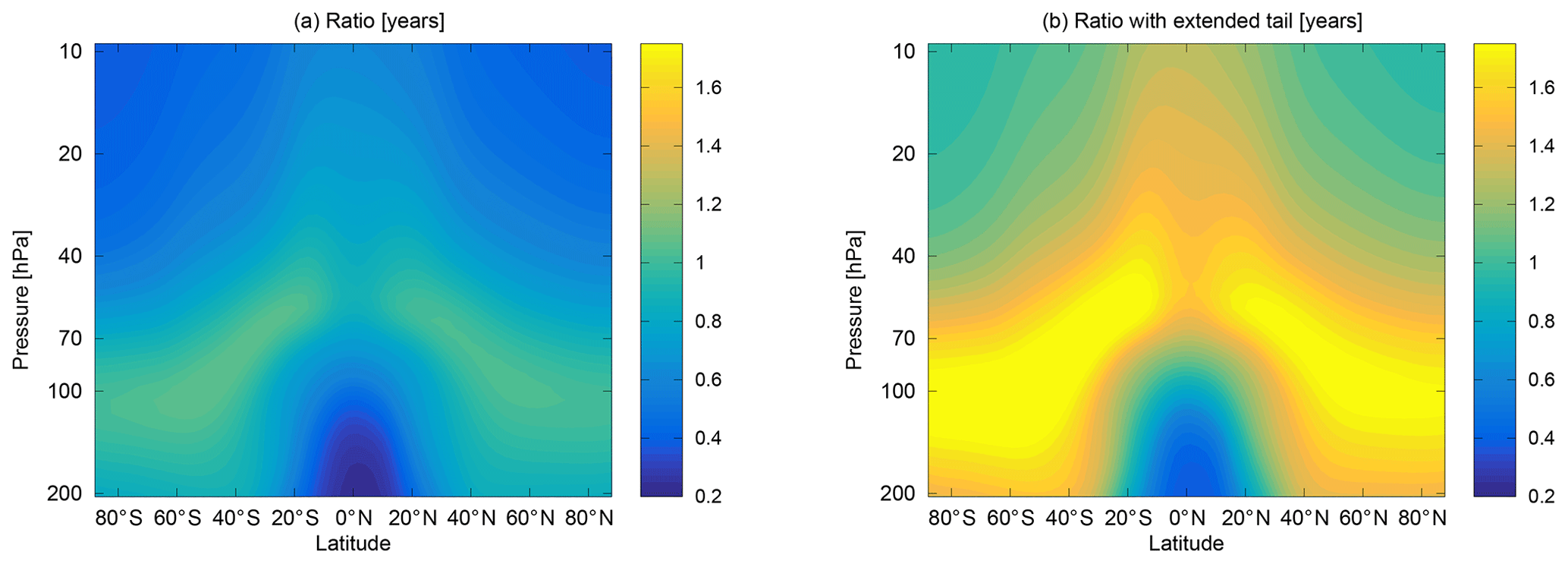
Figure 6Mean ratio $\frac{{\mathrm{\Delta }}^{\mathrm{2}}}{\mathrm{\Gamma }}$ derived from age spectra in the tranPul simulation. (a) For the regular 9.5-year long spectra; (b) with an exponentially extended tail as in Ploeger and Birner (2016).

Download

3.2 Sensitivity of mean AoA and AoA trends to parameter choice in the fit method

As described in Sect. 2.2, mean AoA and its trend were calculated from SF₆ and an ideal linear tracer for the RC1-base-07 simulation for a range of parameters and references for the fit method (explained in Sect. 2.3.1). Since we are considering a self-consistent model world and idealized SF₆ without sinks implemented, we expect perfect agreement between the trends derived from the two tracers.

The fraction of input was varied between 90 %, 95 % and 98 % and the ratio of moments between 0.7, 0.8, 1.0 and 1.25 years. This covers the range for the ratio of moments proposed in Hall and Plumb (1994). Also, the pair of values 98 % and 0.7 years, as applied to the measurements in Engel et al. (2009, 2017), is considered in this selection.

The resulting trends for 40^∘ N and a selection of pressure levels are shown in Fig. 7. Other latitudes show similar behaviour and are therefore not shown. The trend calculation was performed on deseasonalized values and considered autocorrelation (Thompson et al., 2015). The trend of the linear tracer is included in the plots for each parameter choice to make comparison easier, though it does not have any sensitivity to them. Overall, the trends derived from SF₆ are more negative the larger the ratio of moments and closer to zero the larger the fraction of input that is considered. Furthermore, the sensitivity of the trends to the ratio of moments increases when using a lower fraction of input. Intuitively, one might think that the results would be better the more of the reference input is considered (larger fraction of input). However, the fit performed on the reference time series is not weighted by e.g. the spectrum. Therefore taking very long fit intervals takes into account more old air, which only has a small contribution to the actual mean AoA.

Figure 7Overview of the trend in mean AoA derived from SF₆ (dotted lines) and a linear tracer (solid line) for different ratios of moments (x-axis) and fractions of input (colours) at 40^∘ N. The panels show different pressure levels. The trend calculation considered the time series from 1975 to 2011. The error bars show 1σ which is the 68 % confidence levels.

Download

Figure 7 also shows that depending on the pressure level, different selections of ratio of moment and reference input lead to agreement between the trends of the idealized and the SF₆ tracer. The influence of transport and mixing on the age distribution can explain that the best choice for the ratio of moments varies by location.

To build on what was already seen from Fig. 7, Fig. 8 shows the mean absolute deviation of mean AoA derived from SF₆ and the linear tracer in the latitude–height domain for different selections of parameters in the derivation (colours). The white contours show the difference in trends in 10⁻¹ years per decade. Further, in Fig. 8 we also consider spatial distributions of the ratios of moments. Even though we do not have age spectra available for the RC1-base-07 simulation, those from the tranPul simulation are a suitable first estimate for EMAC as a model. We considered the ratio of moments for the 9.5-year long spectra (PulRa sh) and the extended spectra (PulRa) (see Fig. 6).

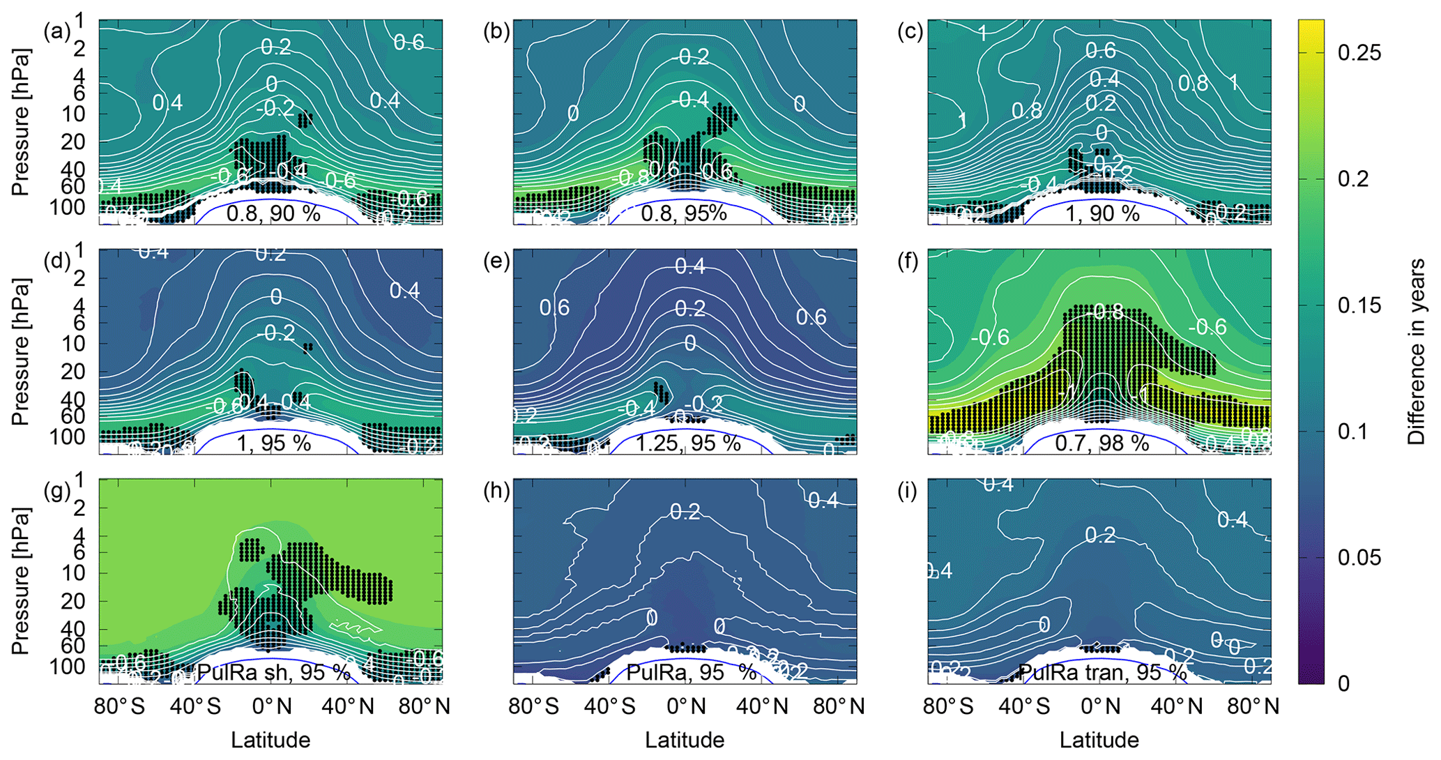
Figure 8Mean absolute deviation of mean AoA calculated from SF₆ from AoA derived from an ideal tracer for a different ratio of moments and fraction of input (colours). The overlaid white contours are the difference in trends in 10⁻¹ years per decade. At the bottom of each panel, the fraction of input and ratio of moments considered in the derivation are stated. PulRa denotes the ratio of moments derived from the tranPul simulation annual mean extended age spectra and PulRa sh is from the 9.5-year spectra. PulRa trans uses the transient extended spectra from that simulation. White areas indicate where the derivation is not applicable. Black stippling shows insignificance of the SF6 trend from zero on the 95 % confidence level. The trend calculation considered the time series from 1975 to 2011. The tropopause and the range 30 K above are excluded, as the AoA calculation is not defined in this region due to the different entry regions into the stratosphere that have to be considered.

Download

It is evident from Fig. 8 that using a fixed ratio of moments for the whole latitude–height domain always leads to deviations in mean AoA and its trends in some regions (panels a–f). Using the ratio of moments derived from the 9.5-year spectra reduces the spatial pattern of deviations (panel g). However, an offset to the actual mean AoA values and trends remains as overall the ratios of moments are underestimated when neglecting the tail. In the range of the balloon-borne observations (5–30 hPa and 32–51^∘ N) this means an average deviation of 4 % in AoA values and 56 % in AoA trend. The ratio of moments derived from the extended age spectra leads to the best agreement across the widest spatial range for both mean AoA and its trend (panel h). Both annual mean ratio of moments and transient ratio of moments were used, though the transient ratio of moments does not show strong further improvement over the annual means (panel i). Using PulRa and 95 % fraction of input provides 1 % average deviation in age values and 12 % deviation in trends in the region of the observations. The spatial dependency of an appropriate ratio of moments might play a role for the measurement application considering that the measurements in Engel et al. (2009) were analysed between 5 and 30 hPa and between 32 and 51^∘ N.

Figure 9 shows an example of the transient ratio of moments at 20 hPa and 40^∘ N. Its trend is drawn, even though it is not significant as the trend is small compared to the variability. The trend of the ratio of moments is negative at all locations, but is mostly not significant. The cycles visible in the ratio of moments can originate from the prescribed QBO and the solar cycle inherent in the prescribed ozone. It is beyond the scope of the current study to examine the large variability in the ratio of moments, but in particular the strong variation with periodicity of about 10 years calls for future investigations. Considering for example Labitzke (2007), it is anticipated that the solar cycle influences the BDC and thereby the shape of the age spectrum. The AoA calculation typically considers about 10 years of reference input. That equates roughly to one cycle in strong variation in ratios of moments which are integrated. That might explain why most improvement in the AoA derivation comes from applying an appropriate spatial distribution of ratios of moments and not from using a transient one.

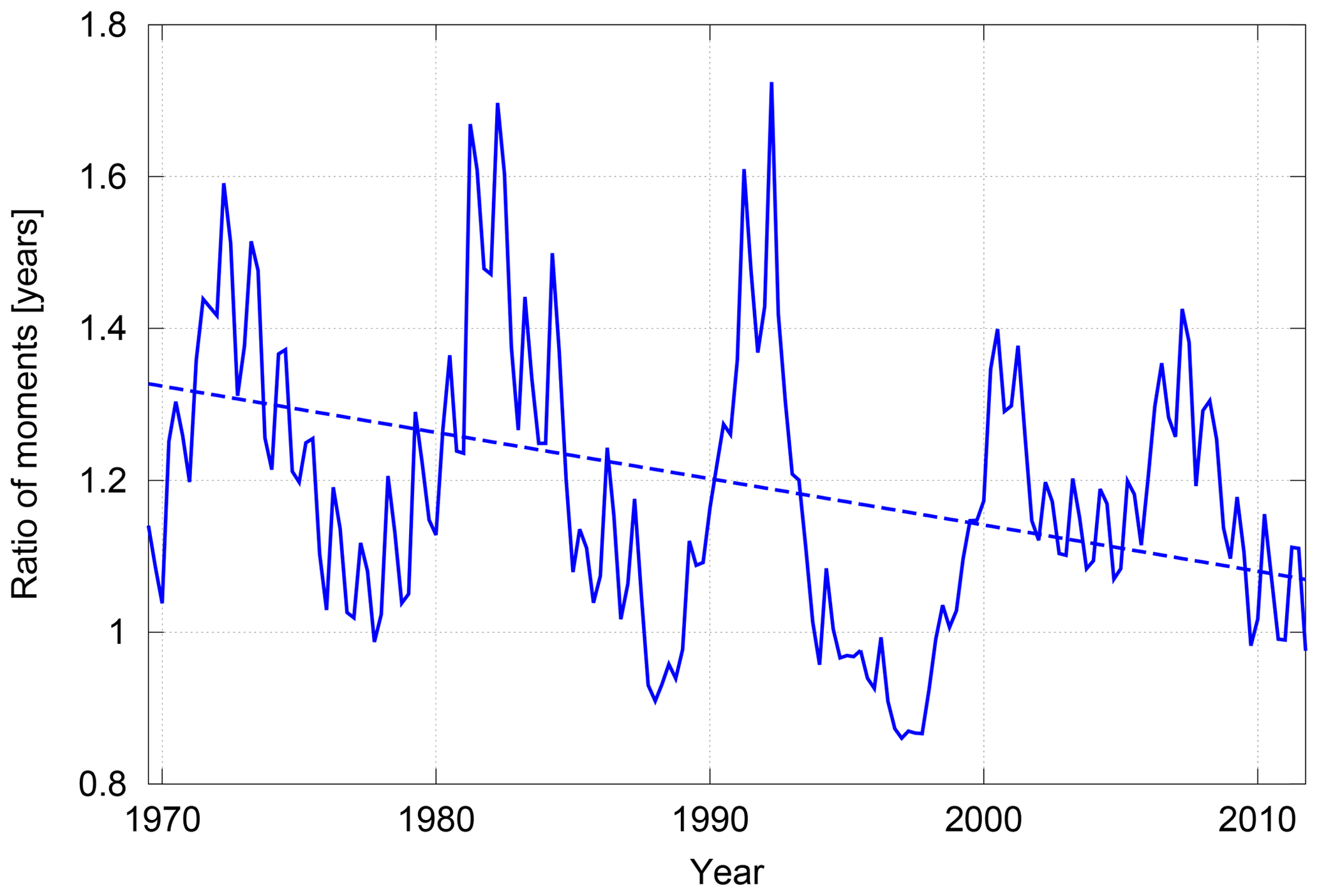
Figure 9Ratio of moments derived from extended age spectra from the tranPul simulation at 20 hPa and 40^∘ N.

Download

As shown in Fig. 8f, the combination of F=98 % and $\frac{{\mathrm{\Delta }}^{\mathrm{2}}}{\mathrm{\Gamma }}=\mathrm{0.7}$ years applied to derive AoA from observations leads to systematic offsets in both mean AoA and the AoA trends between the linear and SF₆ tracer in EMAC. In Fig. 10 the mean AoA trends are shown, which further illustrates the offset in trends. The AoA trends derived from SF₆ with this parameter choice are slightly negative or even positive and insignificant across a wide domain. Calculating the average AoA trend for 98 % and 0.7 years across the spatial range of the observations, i.e. 5–30 hPa and 32–51^∘ N, yields

• −0.13 years per decade ± 0.025 years per decade for the linear tracer;

• −0.057 years per decade ± 0.033 years per decade for the SF₆ tracer.

Hence, averaged across that range, the mean AoA trend derived using those parameters stretches to positive on the 2σ range (95 % confidence). Expressed relatively, these represent average deviations of 4 % in AoA values and 58 % in AoA trend.

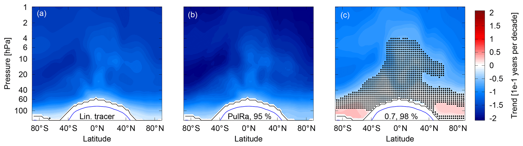
Figure 10Trends of mean AoA from 1975 to 2011 (a) derived from a linear tracer, (b) from SF₆ for the ratio of moments from the extended pulse spectra and 95 % fraction of input and (c) from SF₆ for 0.7-year ratio of moments and 98 % fraction of input. White areas are the areas that cannot be analysed for a trend and black stippling shows insignificance of the trend from zero on the 95 % confidence level using a t-test.

Download

Since the reference location for the AoA calculation can also be varied in model calculations, we checked the effect on the resulting AoA and its trends. However, the different reference locations that have been tested do not show a strong influence on the resulting mean AoA or its trends. For example, an average of the concentration in the area between 20^∘ S and 20^∘ N on the ground and the same range at 100 hPa were used. In that case, the differences in mean AoA are less than half a year and represent the offset time that the air traveled between the different reference locations (not shown). The differences in the trends are below 0.01 years per decade. Both statements refer to the results we obtained for different selections of fraction of input and ratio of moments, i.e. also considering selections that do not perform well overall. However, the reference location is important for quite specific tracer initialization on the ground, for example if the linear AoA tracer is initialized from the poles. In such cases a reference location closer to the tropopause should be used to avoid artifacts of this tracer initialization in the AoA calculation. Since this is not the case for our simulations, we used the ground as a reference in all calculations shown here as it is more applicable to measurements.

We find that the sensitivity of the AoA trends derived from SF₆ to the parameter choice arises predominantly from deviations in mean AoA in earlier years (1970s and 1980s). As an example for this, the left of Fig. 11 shows the mean AoA time series and the derived trend at 20 hPa and 40^∘ N for the combinations 98 % and 0.7 years (red) and 95 % and 1.25 years (blue). The linear tracer is given in black; 95 % and 1.25 years represent a combination with relatively good agreement with the linear tracer in AoA, whereas 98 % and 0.7 years show a strong deviation. For the mean AoA values at this location the length of the fit to the reference time series is around 11 years. Figure 11b shows the differences of the SF₆-derived mean AoA and the linear-tracer-derived mean AoA.

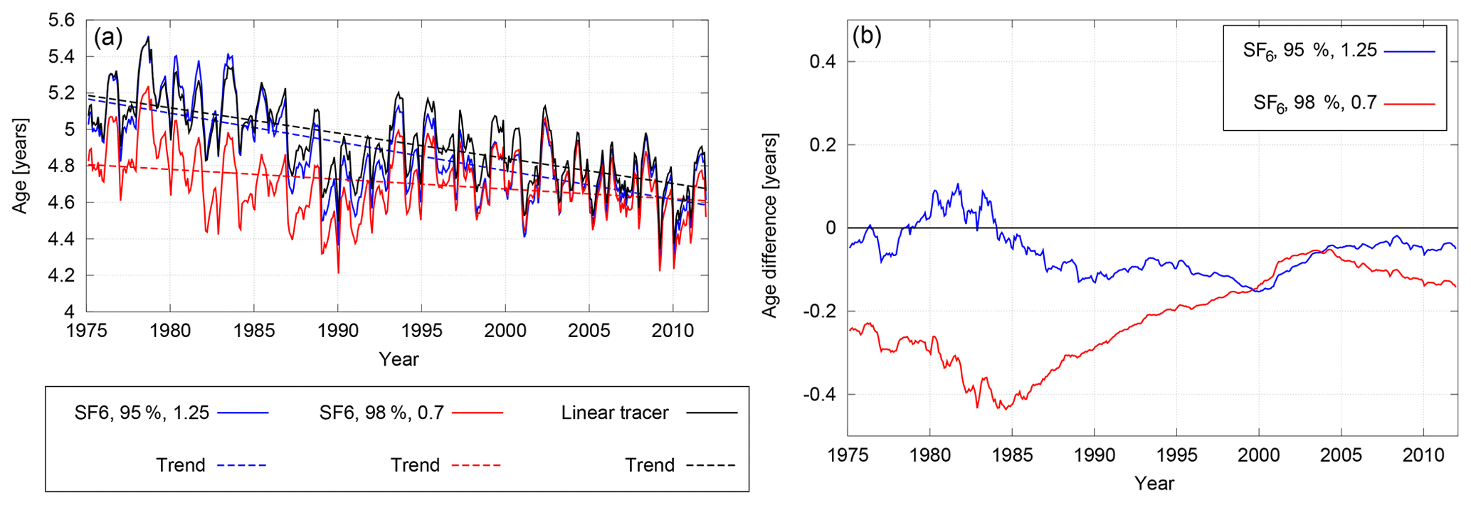
Figure 11(a) Mean AoA and its trend derived from SF₆ for two sets of parameters (red and blue) and from the linear tracer (black) at 20 hPa and 40^∘ N from 1975 to 2011 from the RC1-base-07 simulation. (b) Accordingly mean AoA from the SF₆ tracer minus mean AoA from the linear tracer.

Download

Considering Eq. (7), one explanation for the deviations might be that at the beginning of the reference time series the specific fit coefficients c and b of the second-order polynomial are very sensitive to the fit interval length. Therefore Fig. 12 shows the coefficients dependent on the start date of the fit and the number of years fitted back. The parameters vary slightly more strongly for fits early in the time series. As can be seen from Fig. 12 and already from the SF₆ time series in Fig. 3, the first part of the SF₆ time series is rather linear. In the eighties the second-order contribution is strongest. Afterwards, the slope is rather linear again. Still, the times which show more variation in the coefficients with changing fit interval length do not clearly correspond to the times that the mean AoA derived from SF₆ deviates more from AoA derived from the linear tracer.

Figure 12Coefficients b and c of the second-order polynomial fit to the SF₆ reference time series dependent on the chosen length of fit interval.

Download

Another explanation for the variation in mean AoA might be the sensitivity of the lag time τ to the fit interval length. To be consistent with Engel et al. (2009, 2017), the lag time is determined by approximating the reference time series as a second-order polynomial function of the concentration. Thus depending on the number of years considered, the obtained lag time might vary. This is counterintuitive to what one would expect if the lag time was directly looked up from the concentrations. Figure 13 shows the lag times found for the SF₆ time series for fit interval lengths from 9 to 15 years at the same location as the example in Fig. 11. From roughly 1983 to 1990, τ depends more strongly on the length of the fit interval and varies up to 12 % for the shown range of fit intervals.

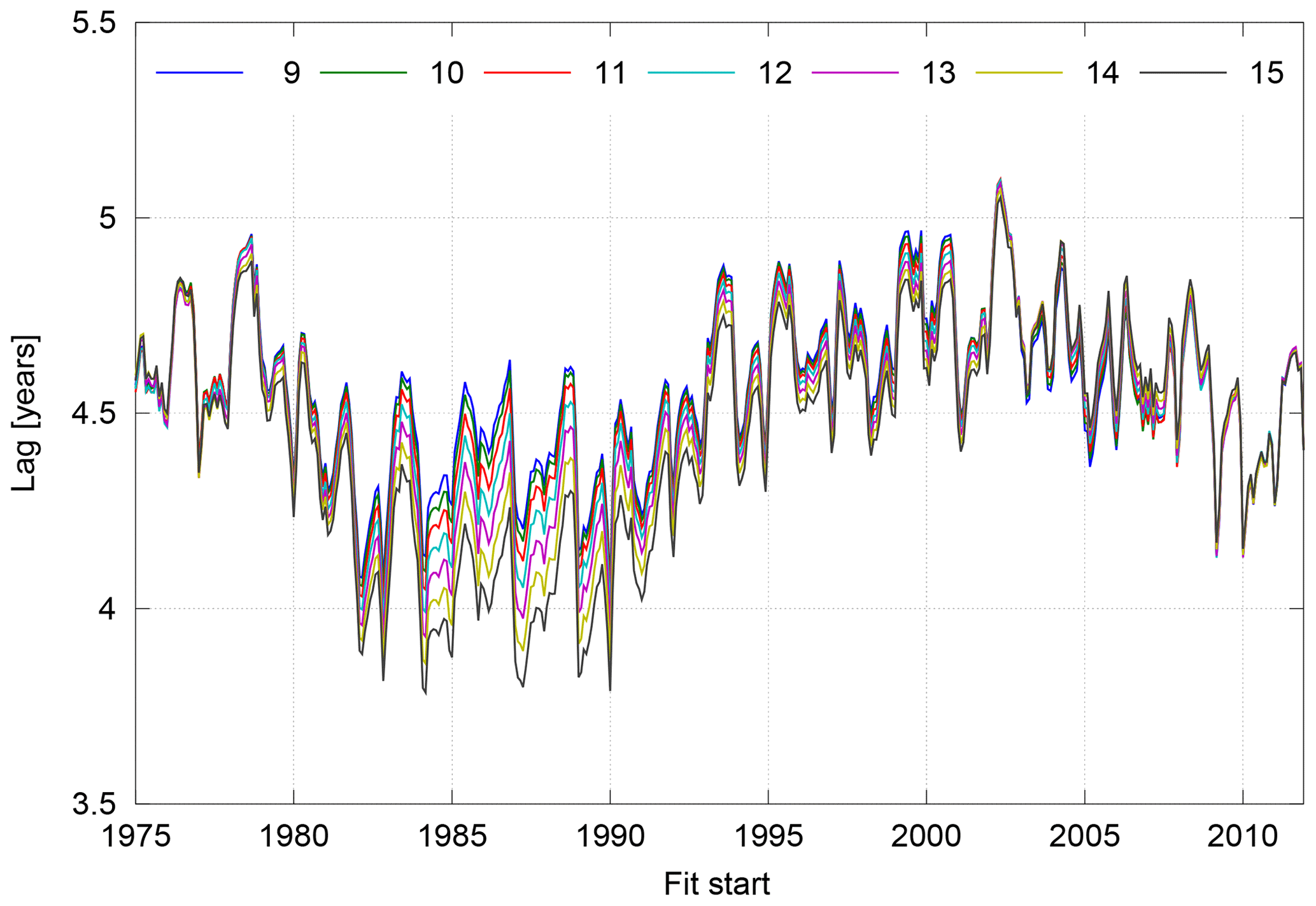
Figure 13Lag time τ for fit interval length 9 to 15 years calculated for the SF₆ time series at 20 hPa and 40^∘ N.

Download

As described when discussing the polynomial coefficients, the SF₆ reference time series slightly bends in the 1980s, which makes the lag time calculation around the late 1980s more sensitive to the fit interval length. The specific years of stronger variation in lag time shift slightly for different locations, dependent on the transport times to that location. As seen from Fig. 11 (right), 1983 to 1990 is also the time of strongest deviation for the non-suitable parameter selection in Fig. 11. The variation in lag time contributes to the variation in mean age in the beginning of the time series dependent on the selection of parameters in the derivation.

Now that the range for the polynomial coefficients b and c from the fit to the SF₆ time series is specifically known from Fig 12, the sensitivity to Γ for the different b and c can additionally be considered. Based on Eq. (7), for a fixed lag time τ, the mean AoA Γ can be calculated for the range of b, c and a different ratio of moments. The results are shown in Fig. 14. Here, τ was chosen to be 4.5 years, which is a reasonable value to apply if we consider the values for τ in Fig. 13.

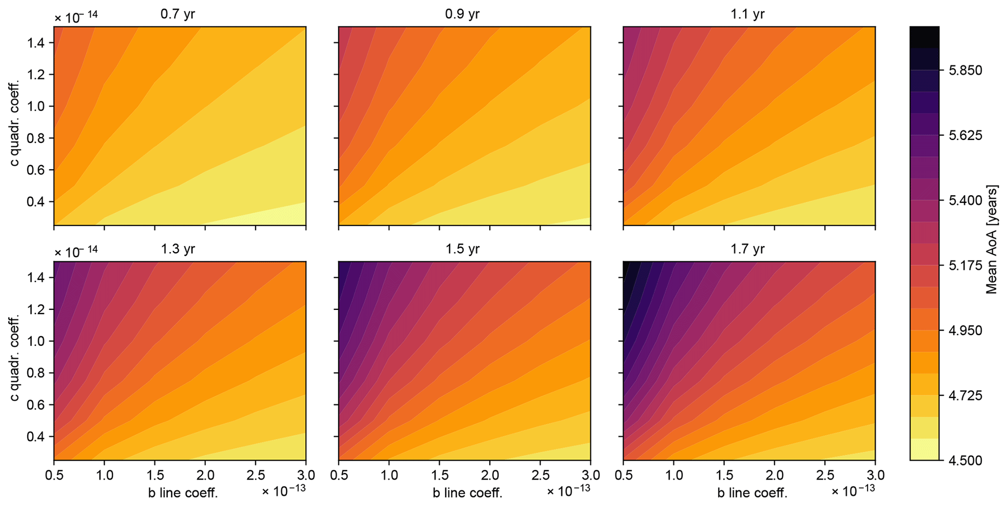
Figure 14Mean AoA Γ for the range of magnitude of the coefficients b and c based on Eq. (7) using the fixed τ=4.5 years. The different panels show the respective ratio of moments (headings).

Download

It can be seen that for b close to zero, Γ becomes more sensitive to the selection of the ratio of moments, as this range shows differences of up to 1 year in mean AoA, for the selected range of ratio of moments from 0.7 to 1.7 years. Most sensitivity of Γ to the ratio of moments is given when in addition c is on the larger end. If we consider the coefficients b and c in Fig. 12, around the year 1980, b tends to be closer to zero and c tends to be on the larger end. This means that around 1980, the sensitivity of mean AoA to the coefficients is very pronounced. Further, the sensitivity is the way around that smaller ratios of moments give smaller mean AoA values. Smaller mean AoA values in the beginning of the time series lead to a less negative AoA trend.

To conclude the considerations why the AoA trend is sensitive to the parameter selection, it can be said that due to the shape of the SF₆ boundary condition the beginning of the AoA time series is particularly sensitive to the parameter selection. The bend in boundary condition around 1980 leads to sensitivity of the lag time τ. Further, the rather flat slope in the beginning of the SF₆ time series implies more sensitivity of mean AoA to the parameter selection then. Therefore, the results about the sensitivity of mean AoA trends to the parameter selection are not dependent on our model or our model resolution.

The latter analyses were done for both SF₆ time series, the one prescribed in the simulation and the one used for calculations from observations. Only the results obtained from the SF₆ time series prescribed in the model are shown here as the results were similar.

3.3 AoA calculations via the convolution method

As described in Sect. 2.3.2, applying the convolution method weights the reference input according to the strength of its influence at a certain observation location. This avoids the influence of an assumption of the fraction of input, so one would expect to see more reliable agreement between AoA and its trends than when applying the fit method. Thus, the convolution method primarily requires an assumption about the ratio of moments of the assumed spectrum. The number of years of reference can just be considered relatively high, e.g. 25 years. As a first example, Fig. 15 shows mean AoA and its trend calculated for ratios of moments 0.7 and 1.25 years from the SF₆ tracer and from the linear tracer. One can see that for 1.25 years of ratio of moments, the agreement between AoA calculated from the linear tracer and from SF₆ becomes very good. However, for a ratio of moments of 0.7 years, the disagreement prevails. Similarly to the fit method, deviations in mean AoA are found in the beginning of the AoA time series maximizing in the 1980s, resulting in an AoA trend that is less negative.

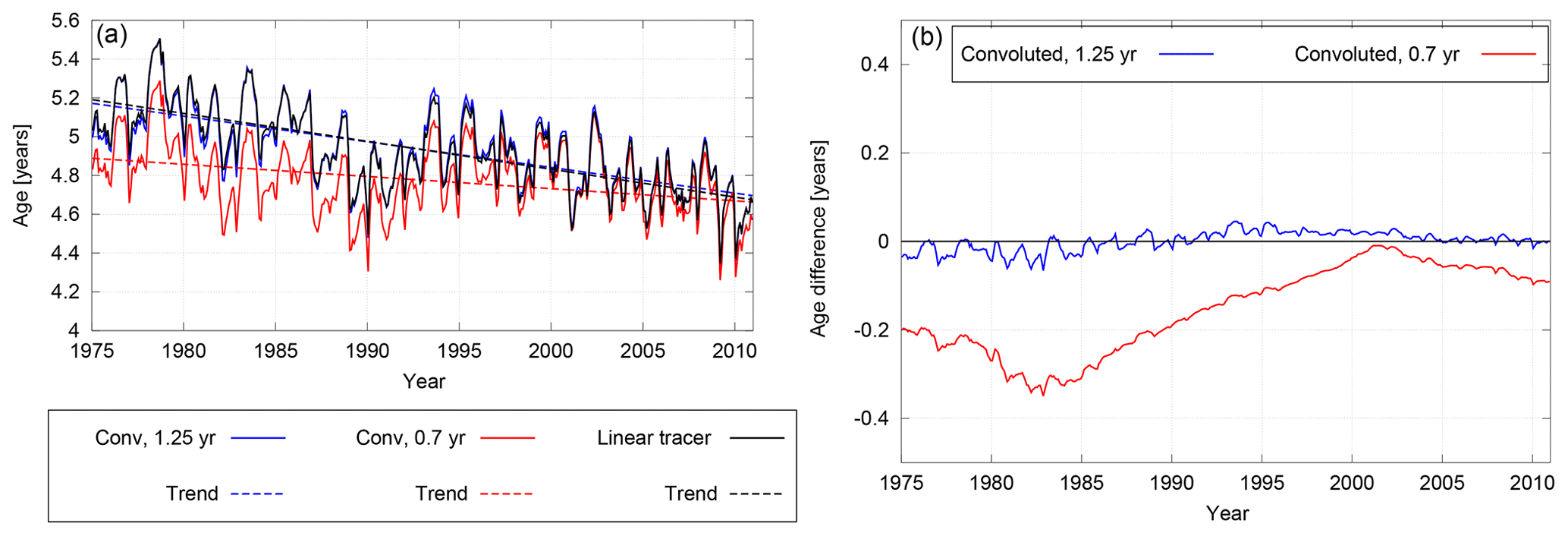
Figure 15(a) Mean AoA and its trend derived from SF₆ using the convolution method for 0.7- and 1.25-year ratios of moments (red and blue) and from the linear tracer (black) at 20 hPa and 40^∘ N from 1975 to 2011 from the RC1-base-07 simulation. (b) The difference in mean AoA derived from SF₆ and the linear tracer.

Download

Similar to Fig. 8, Fig. 16 shows height–latitude plots of the mean absolute deviation between mean AoA calculated using the linear increasing tracer and the SF₆ tracer in colour and the difference in their trends in 10⁻¹ years per decade in white contours. The location of the balloon-borne observations by Engel et al. (2017) is indicated by the red boxes. Here one can see that, overall, a ratio of moments of 0.7 years, which was applied to the balloon-borne observations so far, leads to too small negative or even positive trends, which are insignificant. Specifically, in the range of the observation this is a deviation in mean AoA of 2.8 % and in trend of 54 %. This remains similar to applying this ratio of moments in the fit method. On the other hand, using the ratio of 1.25 years yields very good agreement in the range of the balloon-borne observations (0.3 % in mean AoA, 6 % in trend). Again, using the spatial distribution of ratio of moments derived from the extended model spectra finds good agreement, too (0.4 % in mean AoA, 14 % in AoA trend in the range of the observations).

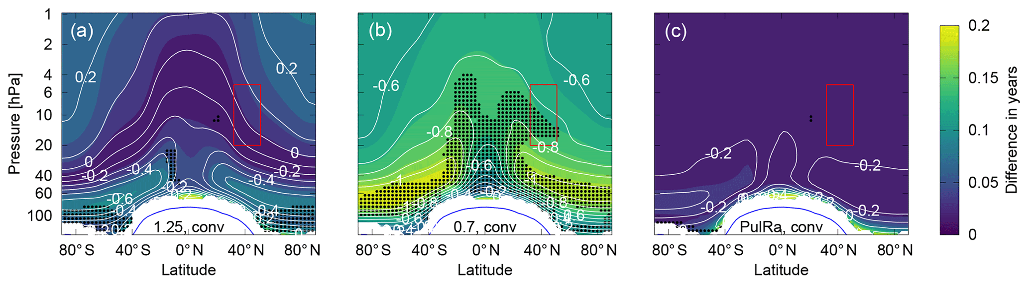
Figure 16As Fig. 8, in colour are the mean absolute deviations of mean AoA calculated from SF₆ from AoA derived from an ideal tracer for every month from 1975 to 2011 for different ratios of moments using the convolution method. (a) is 1.25 years of a ratio of moments and (b) is 0.7 years. PulRa denotes the ratio of moments derived from the tranPul simulation annual mean extended age spectra (c). The white contours are the difference in trends in 10⁻¹ years per decade. White areas indicate where the derivation is not applicable. Black stippling shows the insignificance of the SF₆ trend from zero on the 95 % confidence level. The trend calculation considered the time series from 1975 to 2011. The red box shows the range of the balloon observations.

Download

4.1 Model results

It has been shown here that the variation of the mean AoA trend due to the selection of parameters is larger than the internal variability (e.g. Fig. 7). One might suggest that models still have spin-up effects as the deviations in mean AoA are often in the beginning of the time series. Both simulations, tranPul and RC1-base-07, were started in 1950, but the first 10 years were considered as spin-up. So the data are used starting in 1960, such that the first mean AoA values are calculated for 1975, as the mean AoA calculation fits the reference time series backwards. Previous tests on the effects of spin-up time on AoA in EMAC support that our mean AoA values should not be considerably influenced by spin-up effects for this amount of spin-up. Hence, the differences between models and the observations are not due to spin-up effects in models. We find that the major source of variation in SF₆-derived mean AoA, especially using the fit method, is the selection of parameters.

Another question we consider is whether a second-order fit is appropriate to describe the SF₆ reference time series. Testing higher-order fits shows that the third-order coefficients would be 2 orders of magnitude smaller than the second-order coefficients, and the higher ones even smaller. Therefore, we remain with the second-order assumption, especially since higher-order calculations would require even more assumptions about the transport time distribution which would be even more difficult to constrain in measurement applications.

The convolution method enables us to avoid uncertainties about the amount of time considered and the function that is fitted to the time series. Still, there is a high sensitivity to the ratio of moments, and it remains open which ratio of moments describes the atmosphere best. Still, it is rather certain that larger ratios of moments are more realistic.

4.2 Recalculation of AoA from balloon-borne observations

It is most valuable to put the results derived from the model data concerning parameters and methods of AoA calculations into context by testing whether we see the same tendencies in calculations of observed AoA. The mean age values are recalculated from the observations by Engel et al. (2017) with the fit method with different parameters and the convolution method with different ratios of moments. The results for the trends are given in Fig. 17 and Table 1.

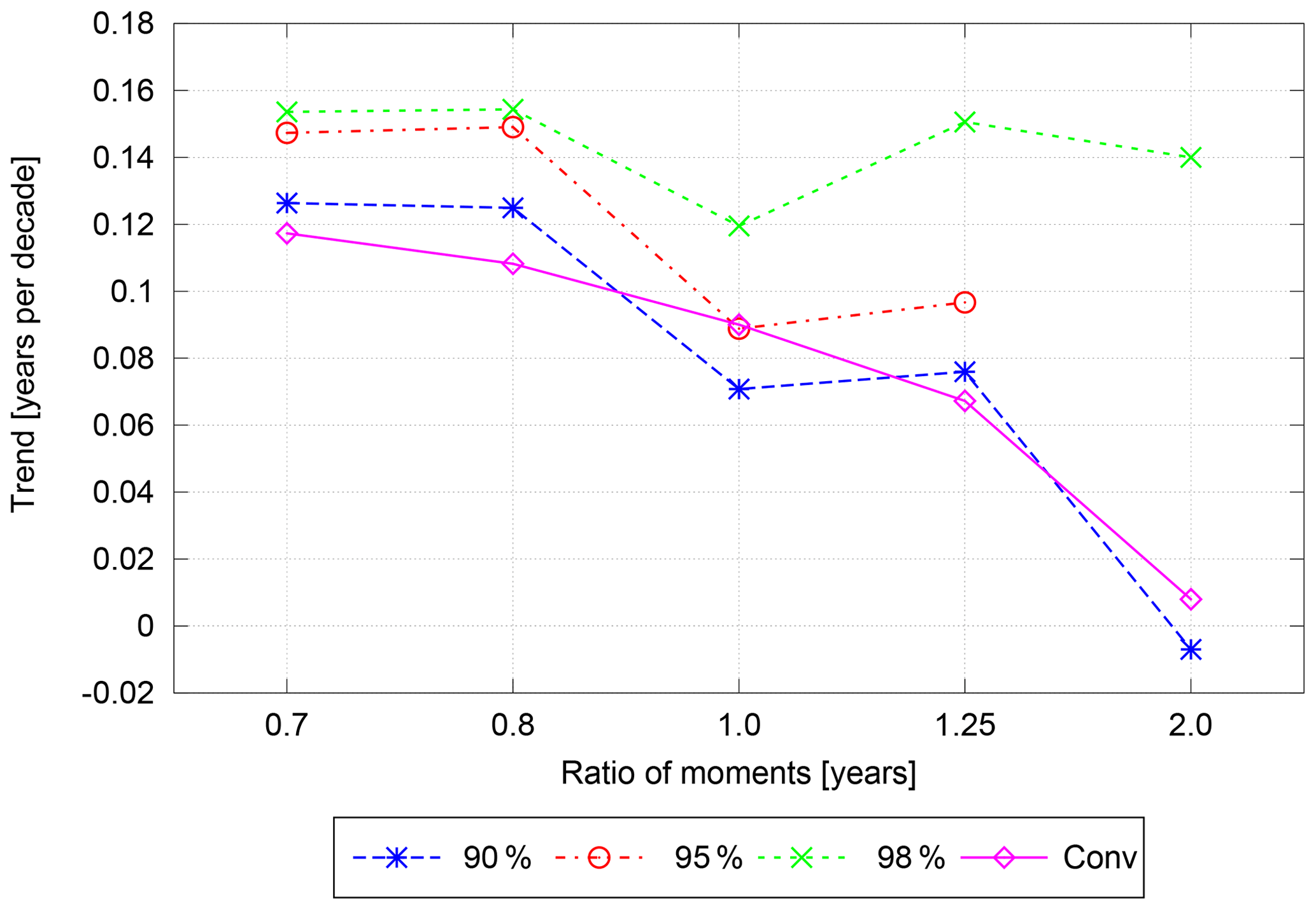
Figure 17Trend in mean AoA derived from the observations for the fit method and the convolution method for the respective fraction of input and ratio of moments.

Download

Table 1AoA trends recalculated from observations using the fit method and convolution method for different parameters. Within the presented decimals, the errors are equal.

Download Print Version | Download XLSX

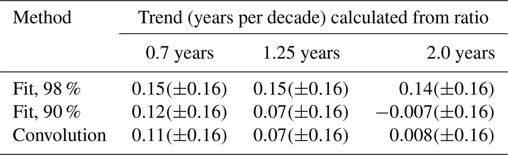
In agreement with what we presented for the model data, there is little influence of the ratio of moments on the trend using the fit method for 98 % fraction of input, as was used in the calculations so far. For 90 % fraction of input, the trend becomes less positive and eventually even slightly negative for larger ratios of moments. Thus, we see the same tendencies towards smaller, respectively more negative trends for larger ratio of moments and smaller fraction of input.

Applying the convolution method for larger ratios of moments gives smaller positive trends, too. This confirms what we have seen from the model data. For both methods for the larger ratio of moments negative trends as seen in the models lay within the margins of error.

Figure 18 presents the AoA time series recalculated from the observations. On the left, the former parameter selection of 98 % and 0.7 years for the fit method is displayed together with the recalculated version for 90 % and 1.25 years. The right shows the spread in mean AoA for the different parameter and methods, that is, 0.7, 0.8, 1.0 and 1.25 years for the convolution method and 90 %, 95 % and 98 % for the fit method. The difference between the largest and smallest AoA values is shown. It becomes clear from the two plots that the beginning of the SF₆ time series is more sensitive in the calculation, as seen for the model data.

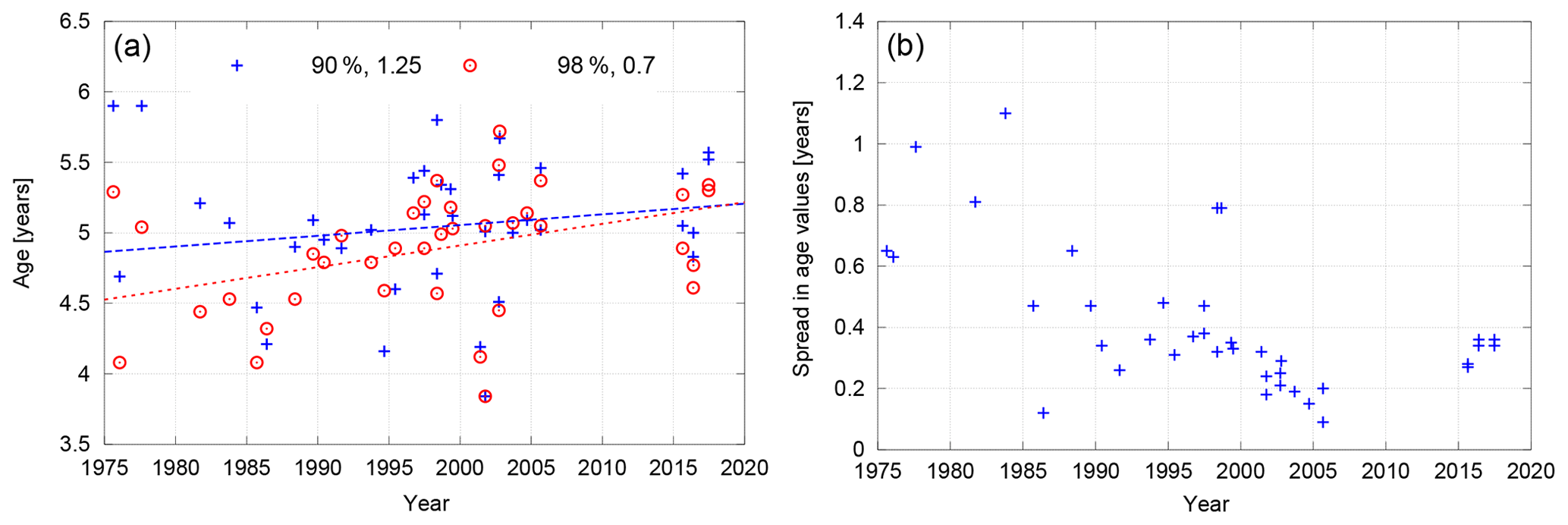
Figure 18(a) Example AoA time series derived from the observations using F=90 %, a 1.25-year ratio of moments and F=98 %, 0.7 years. (b) The difference between maximum and minimum mean AoA found from the observations for the considered parameters (0.7, 0.8, 1.0 and 1.25 years for fit and convolution method and 90 %, 95 % and 98 % for the fit method).

Download

Overall our results show that the selection of parameters helps resolve the difference between model and observation AoA trends. Furthermore, it should be mentioned that Volk et al. (1997) found good agreement with Waugh et al. (1997) using a ratio of moments of 1.25 years for airborne in situ measurements of SF₆. Applying this ratio of moments to the balloon-borne observations results in mean AoA trends that are the same as those of the model, within the margins of error.

However, one should consider that the trend in Engel et al. (2017) was derived from both SF₆ and CO₂ measurements. For calculations using CO₂ measurements methane oxidation is considered to be a minor source. In our discussion, we focused on the specific derivation methods themselves, such that we did not consider CO₂. Consequently, it was favourable to use a SF₆ tracer without mesospheric sinks, in particular since the balloon-borne observations we want to understand are located between 5 and 30 hPa and between 32 and 51^∘ N where the influence of the mesospheric SF₆ sinks has so far been considered to be small. In addition, the combination of CO₂ and SF₆ balloon-borne observations would make an influence of SF₆ sinks on the mean AoA trend less clear. However, the SF₆ sinks are important to consider when discussing the specific differences between mean AoA derived from the global MIPAS satellite SF₆ observations and models as Linz et al. (2017) did, especially in the light of recent studies that report shorter lifetimes for SF₆ than assumed so far (Leedham Elvidge et al., 2018; Ray et al., 2017).