the Creative Commons Attribution 4.0 License.
the Creative Commons Attribution 4.0 License.
 | 22 Jul 2020
Analysis of 24 years of mesopause region OH rotational temperature observations at Davis, Antarctica – Part 2: Evidence of a quasi-quadrennial oscillation (QQO) in the polar mesosphere
W. John R. French
Andrew R. Klekociuk
Frank J. Mulligan
Observational evidence of a quasi-quadrennial oscillation (QQO) in the polar mesosphere is presented based on the analysis of 24 years of hydroxyl (OH) nightglow rotational temperatures derived from scanning spectrometer observations above Davis research station, Antarctica (68∘ S, 78∘ E). After removal of the long-term trend and solar cycle response, the residual winter mean temperature variability contains an oscillation over an approximately 3.5–4.5-year cycle with a peak-to-peak amplitude of 3–4 K. Here we investigate this QQO feature in the context of the global temperature, pressure, wind, and surface fields using satellite, meteorological reanalysis, sea surface temperature, and sea ice concentration data sets in order to understand possible drivers of the signal. Specifically, correlation and composite analyses are made with data sets from the Microwave Limb Sounder on the Aura satellite (Aura/MLS v4.2) and the Sounding of the Atmosphere using Broadband Emission Radiometry instrument on the Thermosphere Ionosphere Mesosphere Energetics Dynamics satellite (TIMED/SABER v2.0), ERA5 reanalysis, the Extended Reconstructed Sea Surface Temperature (ERSST v5), and Optimum-Interpolation (OI v2) sea ice concentration. We find a significant anti-correlation between the QQO temperature and the meridional wind at 86 km altitude measured by a medium-frequency spaced antenna radar at Davis (R2∼0.516; poleward flow associated with warmer temperatures at K (ms−1)−1). The QQO signal is also marginally correlated with vertical transport as determined from an evaluation of carbon monoxide (CO) concentrations in the mesosphere (sensitivity 0.73±0.45 K ppmv−1 CO, R2∼0.18). Together this relationship suggests that the QQO is plausibly linked to adiabatic heating and cooling driven by the meridional flow. The presence of quasi-stationary or persistent patterns in the ERA5 data geopotential anomaly and the meridional wind anomaly data during warm and cold phases of the QQO is consistent with tidal or planetary waves influencing its formation, which may act on the filtering of gravity waves to drive an adiabatic response in the mesosphere. The QQO signal plausibly arises from an ocean–atmosphere response, and appears to have a signature in Antarctic sea ice extent.
- Article
(22525 KB) - Companion paper
-
Supplement
(1153 KB) - BibTeX
- EndNote


In Part 1 of this study (French et al., 2020) we quantify the solar cycle and long-term trend in 24 years of hydroxyl (OH) rotational temperature measurements from Davis research station, Antarctica, and observed that the winter mean residual temperatures revealed a periodic oscillation over an approximately 4-year cycle with an amplitude of 3–4 K. While periodic oscillations occur on many timescales in the atmosphere from minutes to years (gravity waves; tides; planetary waves; seasonal variations; quasi-biennial oscillation, QBO; El Niño–Southern Oscillation, ENSO; Pacific Decadal Oscillation, PDO; solar cycle), the approximately 4-year period of this quasi-quadrennial oscillation (QQO) is unusual in terms of weather and climate modes. Here we seek to characterize the features and extent of the observed behaviour and to examine correlation and composites with several atmospheric parameters which might suggest a possible mechanism for the phenomenon.
References to quasi-quadrennial variability in Earth's climate system have previously been reported by Jiang et al. (1995), who found both quasi-quadrennial (52 months) and quasi-biennial (24 and 28 months) oscillation modes in equatorial (4∘ N–4∘ S) sea surface temperature (SST) and 10 m zonal wind fields over the 1950–1990 interval. They found the variation consistent with a “devils staircase” interaction between the annual cycle and ENSO. Liu and Duan (2018) use principal oscillation pattern analysis over the 1979–2013 era to also identify a QQO (48 months) in global SST anomaly which is dominant in the equatorial Pacific Ocean region. Liu and Xue (2010) investigated the relationship between ENSO and the Antarctic Oscillation (AAO) index with empirical orthogonal function analysis in sea level pressure anomalies from 1951–2002. They concluded that ENSO plays a key role in the phase transition of AAO at the quasi-quadrennial timescale. Pisoft et al. (2011) point out that the quasi-quadrennial oscillations that have been reported are almost always associated with the ENSO phenomenon and variations in sea surface temperatures or the wind field over equatorial areas. Pisoft et al. (2011) applied a two-dimensional wavelet transform technique to changes in 500 hPa temperature fields in two 50-year reanalysis data sets (ERA-40 and NCEP–NCAR) and established the presence of a distinct QQO and a quasi-decadal oscillation in addition to the annual and semi-annual cycles. Their analysis showed that the QQO is present in at least 15 of 50 years in both reanalysis data sets not only in the equatorial zone (30∘ S–30∘ N) but also over a significant area of the globe including high latitudes. Both reanalysis data sets showed relatively high QQO wavelet power north of the Bellingshausen and Amundsen seas, over the Bering Sea, and over North America (north of ∼45∘ N). A region of relatively high wavelet power was detected north of the Mawson and Davis seas near Antarctica in ERA-40 only.
There are relatively few reports of observations of multi-year variability in the mesosphere and higher altitudes, and as far as we are aware, the existence of a QQO in the high-latitude mesopause region as discussed here has not previously been reported. Offermann et al. (2015) reported multi-annual temperature oscillations in central Europe detected in Sounding of the Atmosphere using Broadband Emission Radiometry (SABER) data during the period 2002–2012, which were reproduced in simulations by the Hamburg Model of the Neutral and Ionized Atmosphere (HAMMONIA) chemistry climate model (Schmidt et al., 2006) and the Community Earth System Model – Whole Atmosphere Community Climate Model (CESM-WACCM); Marsh et al., 2013). Periods of 2.2–2.4, 3.4, and 5.5 years were present in the SABER data over a range of altitudes from 18 to 110 km. Perminov et al. (2018) reported statistically significant periods of OH* temperature variations at 3 years and 4.1 years (with amplitudes of 1.3±0.2 and 0.6±0.2 K respectively) from a Lomb–Scargle analysis of 17 years (2000–2016) at Zvenigorod, Russia. Reid et al. (2014) detected significant periodicities at 4.1 years in O(1S) emission intensity and ∼3 years in the OH emission intensities by performing a Lomb–Scargle analysis of a 15-year series of observations at Adelaide, Australia. However, Perminov et al. (2018) and Reid et al. (2014) do not offer causes of these periodicities.
The outline of this paper is as follows. In Sect. 2 we review the Davis OH rotational temperature measurements (described in Part 1 of this study) and the derived residual temperatures which contain the QQO feature. In Sect. 3 we explore correlation and composite analyses of the QQO signal using satellite and meteorological reanalysis data sets. A discussion of the results, summary, and conclusions drawn is given in Sects. 4 and 5. Additional figures are presented in the Supplement.
As for Part 1 we use the following terminology for the analysed temperature series. From the measured temperatures and their nightly, monthly, seasonal, or winter means, temperature anomalies are produced by subtracting the climatological mean or monthly mean (we fit a solar cycle and linear long-term trend to the anomalies); residual temperatures additionally have the solar cycle component subtracted and detrended temperatures have both the solar cycle component and the long-term linear trend subtracted.
2.1 OH(6–2) rotational temperatures
Scanning spectrometer observations of the OH airglow (6–2) band have been made at Davis station, Antarctica (68.6∘ S, 78.0∘ E) for each winter season over the last 24 years (1995–2018) to provide a time series of rotational temperatures (a layer weighted proxy of atmospheric temperatures near 87 km altitude). The solar cycle and long-term linear trend in this temperature series are examined in Part 1 of this study (French et al., 2020). Fitting a solar cycle (using 10.7 cm solar flux) and linear long-term trend model to the winter mean temperature anomalies (nightly mean temperatures averaged over day-of-year 106 to 259 with mean climatology subtracted) yields a solar cycle response coefficient S of 4.30±1.02 K per 100 sfu (95 % confidence limits 2.2 K per 100 sfu <S<6.4 K per 100 sfu) and a long-term linear trend L of K per decade (95 % confidence limits −0.14 K per decade <L<−2.26 K per decade). However, only 58 % (R2) of the year-to-year variability is described by this model (see Fig. 3 of Part 1). Residual temperatures (solar component removed) are shown in Fig. 1a and the detrended temperatures (solar component and long-term linear fit removed) in Fig. 1b. The QQO signal is apparent, with a peak–peak amplitude of 3–4 K. A sinusoid fit to the residual temperatures is provided as a guide and has a peak-to-peak amplitude of 3.0±0.7 K and a period of 4.2±0.1 years. A wavelet analysis of the residual time series shown in Fig. 1c reveals an oscillation period increasing from ∼3.5 years in 2000 to 4.5 years in 2013.
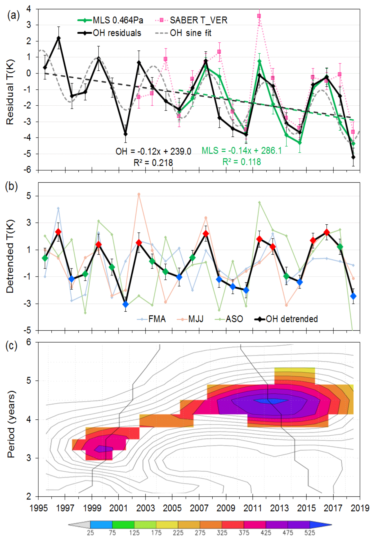
Figure 1(a) Davis OH winter mean residual (solar response removed) temperatures (black line, standard error in mean error bars, dashed linear fit) compared with Aura/MLS (AMJJAS) mean residual temperatures for 0.0046 hPa (green line, standard error-in-mean error bars, dashed linear fit) and TIMED/SABER (pink dotted line, standard error-in-mean error bars). Grey dotted line is a sinusoid fit (peak–peak amplitude 3.0±0.1 K period 4.2±0.7 years) provided as a guide. (b) Detrended Davis OH winter mean temperatures (AMJJAS) (black line, long-term linear fit removed) compared to FMA, MJJ, and ASO monthly averages (red, green, and blue points mark warm, mid, and cold years respectively for composite studies). (c) A Morlet wavelet transform (order 6) of the detrended Davis OH winter mean temperatures. Coloured sections are power above 90 % significance level. The black line indicates the cone of influence; points outside have been influenced by the boundaries of the time series.
We have attempted to examine the seasonal variability of the QQO signal by dividing averages into the intervals FMA (February–March–April), MJJ (May–June–July), and ASO (August–September–October) (also plotted in Fig. 1b). While these shorter-term averages obviously suffer from greater uncertainty, there is a suggestion that the QQO is strongest over the winter months MJJ, mid-range in ASO, and less apparent in the FMA interval.
2.2 Aura/MLS temperature profiles
Long-term temperature data for the mesopause region are available from two satellite instruments; the Microwave Limb Sounder on the Aura satellite (Aura/MLS) and the SABER instrument on the Thermosphere Ionosphere Mesosphere Energetics Dynamics (TIMED) satellite. Hydroxyl layer equivalent temperature measurements from these instruments are overlaid in Fig. 1a.
Aura/MLS temperatures are derived from observations of thermal microwave emissions near the oxygen spectral lines of O2 (118 GHz) and O18O (234 GHz). The instrument scans the Earth's limb every 24.7 s and the retrieval algorithm (for version v4.2 level 2 used here) produces useful temperature profiles on a fixed vertical pressure grid from 316 hPa (∼8 km) to 0.001 hPa (∼97 km) over the latitude range 82∘ S–82∘ N with about 14 orbits per day. The along-track resolution is typically 165 km through the stratosphere to 220 km at the top of the mesosphere. The vertical resolution is defined by the full width at half maximum of the averaging kernels and varies from 5.3 km at 316 hPa to 9 km at 0.1 hPa and up to 15 km at 0.001 hPa (Schwartz et al., 2008). We also use profiles of carbon monoxide (CO) mixing ratio, which are scientifically useful between 215 to 0.0046 hPa and have a similar vertical and horizontal resolution to the temperature measurements.
For comparison with the Davis OH temperatures we selected Aura/MLS profiles acquired within 500 km of Davis station (about 60 coincident samples per month) between 2005 (Aura launched in July 2004) and 2018, applied selection criteria according to the quality control recommendations described in Livesey et al. (2020) and averaged over the winter months April to September (AMJJAS; similar to the averaging period for the Davis winter mean) at the native Aura/MLS retrieval pressure level of 0.00464 hPa. The 0.00464 hPa pressure level statistically provides the best chi-squared fit, comparing temperature anomalies of Aura/MLS to the Davis anomalies, and is in good agreement in absolute terms to the OH(6–2) temperatures we derive using Langhoff et al. (1986) transition probabilities (see discussion in Part 1; French et al., 2020). The Aura/MLS AMJJAS mean temperature residuals are overlaid in Fig. 1a (green line from 2005); the solar cycle component is removed in the same way as for the OH data. For comparison, regression values for Aura/MLS (2005–2018) are 3.4±2.3 K per 100 sfu for the solar term and K per decade for the long-term trend (but neither term is significant at the 95 % level; R2=0.2). If the solar response coefficient derived for the 24 years of OH measurements is used to compute residuals, the Aura/MLS long-term linear trend becomes K per decade (R2=0.12). The Aura/MLS measurements show very good agreement with the OH measurements, both in terms of the long-term linear fit to the residuals and in the magnitude and pattern of the QQO feature over its last three cycles.
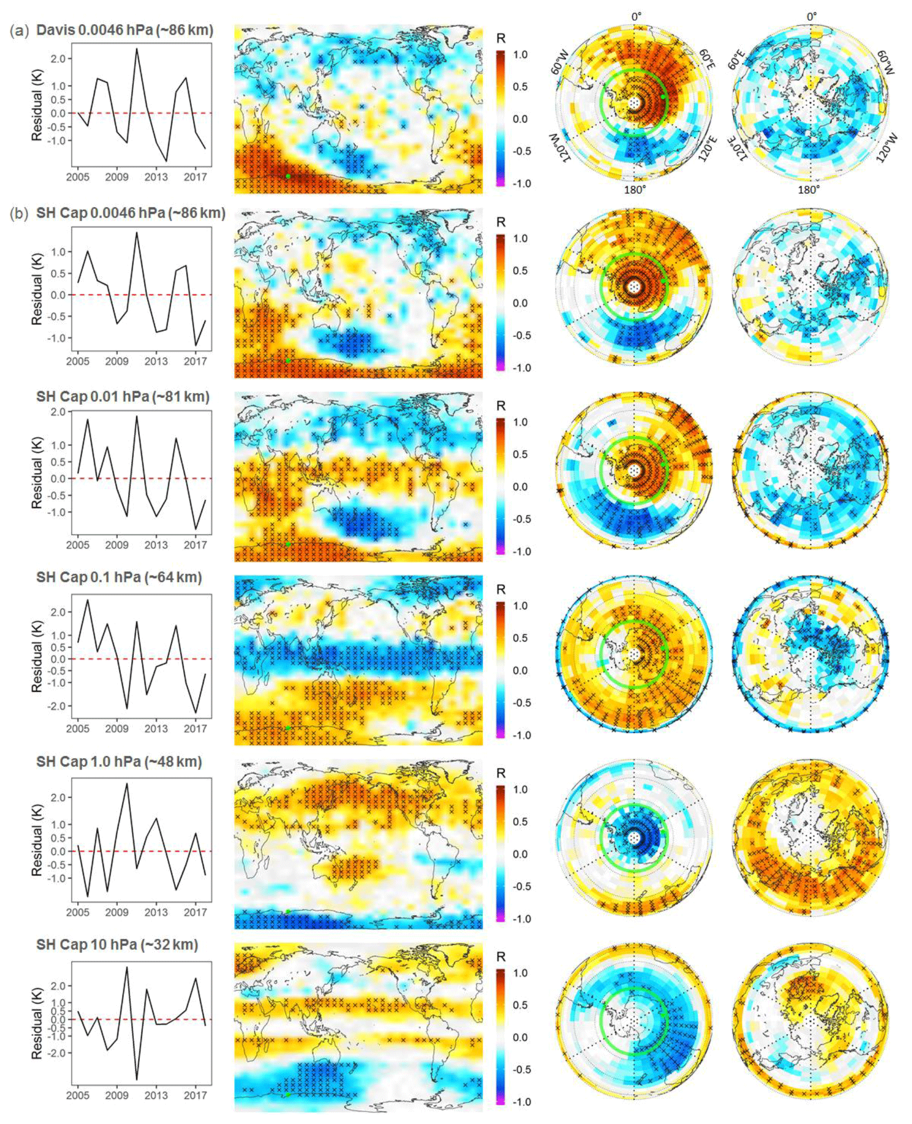
Figure 2(a) Correlation of the Aura/MLS 0.0046 hPa grid box QQO residual temperature signal at Davis (left-hand time series panel) with each grid box of the Aura/MLS 0.0046 hPa global temperature field gridded in bins. Equi-rectangular and polar projections of the correlation (R) are shown (crossed grid cells are significant at the 90 % level). Davis location indicated by green dot. (b) Correlation of the 0.0046 hPa SH polar cap winter average (65–85∘ S; AMJJAS; green circle) with each grid box of the Aura/MLS temperature fields at various pressure levels as indicated.
2.3 TIMED/SABER profiles
The SABER instrument measures Earth limb emission profiles over the 1.27–17 µm spectral range from the TIMED satellite, which was launched in December 2001 into a circular orbit at 625 km altitude and 74∘ inclination to the Equator (Russell III et al., 1999). The satellite undergoes a yaw cycle every 60 d, alternating coverage of latitude bands 54∘ S–82∘ N and 82∘ S–54∘ N and precessing slowly to complete 24 h local time over the yaw interval. Temperature is retrieved over an altitude range of 10–105 km, with a vertical resolution of about 2 km and an along-track resolution of 400 km from 15 and 4.3 µm carbon dioxide (CO2) emissions (Mertens et al., 2003). Generally, errors in the retrieved temperatures in the mesopause region are estimated to be in the range ±1.5–5 K (García-Comas et al., 2008).
SABER also measures a volume emission rate (VER) from a radiometer sensitive over the 1.56–1.72 µm spectral range (OH-B channel) which includes mostly the OH(4–2) and OH(5–3) bands. SABER v2.0 Level 2B data are used in this study. We use a Gaussian fit to the VER to derive weighted average OH layer equivalent temperatures (T_VER; as for French and Mulligan, 2010). While the VER layer weighting profile from the OH-B channel is a combination of vibrational levels and , and not the v'=6 level measured here, the difference from the profile in terms of peak altitude is not expected to be greater than 1 km, compared to the ∼8 km full width at half maximum (FWHM) of the layer (McDade, 1991; von Savigny et al., 2012). The resulting temperature offset is much less than 1 K.
As for Aura/MLS we average all SABER profiles within a 500 km radius of Davis station that fall within the winter averaging window. Due to the satellite yaw cycle this limits SABER observations to two intervals (days of the year 75–140 and 196–262) and the days prior to 106 and after 259 are rejected as being outside the OH winter interval. Thus, only days 106–140 and 196–259 are comparable between SABER and Davis OH over the winter interval and days 141–195 (21 May to 14 July) are excluded. As for the OH temperatures and Aura/MLS, a fit of solar cycle (F10.7) and linear trend terms is made. Regression values for SABER for 2002–2018 are 3.4±1.8 K/100 sfu for the solar term and K per decade for the long-term trend using this model. Neither term is statistically significant at the 95 % level (R2=0.22). The solar term is significant at the 90 % level.
Both the OH peak altitude and the OH T_VER (ignoring the solar term) show slightly negative trends over the period 2002–2018 ( km yr−1, R2=0.09 and K yr−1, R2=0.09 respectively), but they are not statistically significant. Plots of the OH peak altitude and OH T_VER time series and the anti-correlation relationship are provided in Fig. S1 of the Supplement. There is a slight anti-correlation between OH peak altitude and T_VER ( K/km, R2=0.1), but once again, the value is not statistically significant.
The derived SABER residual mean temperatures are also plotted in Fig. 1a (pink dotted line) for the years 2002–2018. Given that the yaw cycle excludes days 141–195 from the winter averaging in these data, in general the SABER residual temperatures also reproduce the QQO variation, except that 2011 appears to be anomalously warm (by ∼3 K). The OH peak altitude derived from the SABER OH_VER profile also shows an anomalously low layer altitude for 2011 (lowest winter mean altitude in the 2002–2018 year record; see Fig. S1).
2.4 ECMWF/ERA5
As discussed in the introduction, reported oscillations on a quasi-quadrennial scale have almost always been associated with ENSO and its interactions in near-surface equatorial pressure, wind, and sea surface temperature fields. To investigate the possible connection to the Antarctic mesopause QQO observation, we perform correlation and composite analyses using the European Centre for Medium Range Weather Forecasting (ECMWF) ERA5 reanalysis products (Copernicus Climate Change Service, 2017; https://apps.ecmwf.int/data-catalogues/era5/?class=ea, last access: 3 July 2020). These include global monthly average geopotential height and wind components provided on 37 pressure levels (surface to 1 hPa) at a grid point resolution.
2.5 ERSST and OISST
The SSTs used in this study are from the National Oceanic and Atmospheric Administration (NOAA) Extended Reconstructed Sea Surface Temperature (ERSST v5; https://www.ncdc.noaa.gov/data-access/marineocean-data/extended-reconstructed-sea-surface-temperature-ersst-v5, last access: 3 July 2020) monthly data set derived from the International Comprehensive Ocean–Atmosphere Dataset (ICOADS). These are available globally, extending from January 1854 to the present at a grid resolution with spatial completeness enhanced using statistical methods (Huang et al., 2017).
For sea ice cover, we also use the NOAA Optimum Interpolation Sea Surface Temperature (OISST) V2 product, available as monthly means on a 1∘ global grid using in situ and satellite SSTs plus SSTs simulated by sea ice cover. (Reynolds et al., 2002; https://www.esrl.noaa.gov/psd/data/ gridded/data.noaa.oisst.v2.html, last access: 3 July 2020)
The spatial extent of the QQO signal observed at Davis is explored with the Aura/MLS data set for the 2005–2018 interval of concurrent observations. These data are averaged into (latitude × longitude) grid cells. In Fig. 2a we correlate the Aura/MLS AMJJAS temperature residual time series for the grid cell over Davis (14 years; time series plotted in the left-hand panel) with each grid cell of the Aura/MLS AMJJAS temperature residual at 0.0046 hPa. The three map panels show correlation coefficient (R) in equi-rectangular, Southern Hemisphere (SH) and Northern Hemisphere (NH) projections. The correlation colour scale is common to all maps and crossed grid cells show significance at the 90 % level. The Davis QQO signal shows a significant positive correlation with a large part of the east Antarctic and southern Indian Ocean sectors and significant anti-correlation in the Southern Ocean near New Zealand. In the NH summer, there is a general region of negative correlation at mid- to high latitudes, indicating that the QQO has opposite phases in the two hemispheres. We return to compare the response between hemispheres in Sect. 4.5.
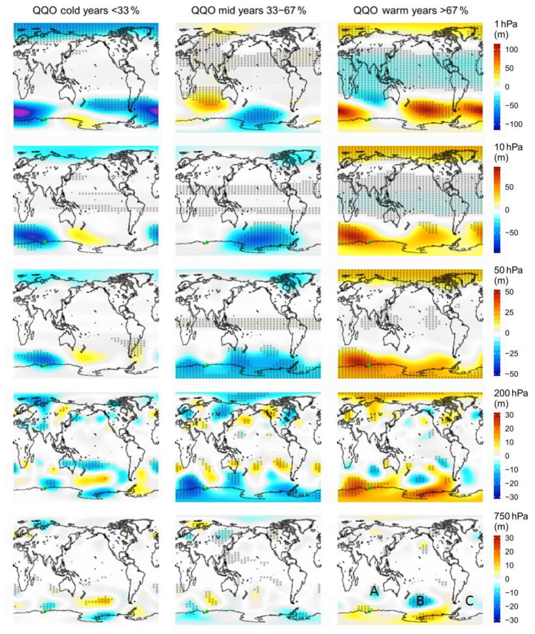
Figure 3Composites of the ERA5 (AMJJAS) geopotential anomaly, for cold, mid, and warm years of the Davis detrended winter average QQO signal. Pressure levels are indicated on the right-hand colour bar. The colour scales are in metres of geopotential height. Hashed areas on the plots are significant at the 90 % level.
Extending this analysis, Fig. 2b shows the correlation between the mean Aura/MLS temperature of the polar cap (65–85∘ S), which has a variation similar to that shown in Fig. 2a for Davis (left-hand panel), with Aura/MLS temperatures for each grid box on a range of pressure levels representative of the mesopause region, mesosphere, stratopause region, and stratosphere. It is apparent that the QQO signal observed at Davis extends over the majority of the polar cap and through most of the mesosphere down to at least the 0.1 hPa level with a similar amplitude (3–4 K peak-to-peak) and phase. Significant anti-correlation of the QQO signal then occurs in the upper stratosphere (pressure range 1–10 hPa) in the polar cap and Southern Ocean, while a significant positive correlation occurs in the region of the subtropical jets at 10 hPa. Time series of Aura/MLS (AMJJAS) polar cap (65–85∘ S) averages at additional pressure levels are provided in Fig. S2 to complement the selected levels in Fig. 2b and detail the transition in wave pattern from mesosphere to stratosphere.
We further examine the Davis QQO signal using correlation and composite analysis with the ECMWF/ERA5 reanalysis data and NOAA/ERSST v5 data described above. Figure 3 shows the composites of the ERA5 geopotential height anomaly (with respect to the 1995–2018 climatology) averaged over AMJJAS for the 33rd percentile (“cold” years), the 67th percentile (“warm” years), and the remaining “mid” years (between the 33rd and 67th percentiles) of the detrended Davis hydroxyl temperature winter average QQO signal at pressure levels of 750, 200, 50, 10, and 1 hPa. The first two pressure levels are globally generally within the troposphere, and the other levels are generally within the stratosphere. The cold years (threshold −0.99 K) and their detrended temperature values (in parenthesis) are 1997 (−1.166), 2001 (−3.039), 2005 (−1.023), 2008 (−1.188), 2009 (−1.738), 2010 (−1.998), 2014 (−1.381), and 2018 (−2.451). The warm years (threshold 1.24 K) and their detrended temperature values (in parenthesis) are 1996 (2.325), 1999 (1.399), 2002 (1.523), 2007 (2.210), 2011 (1.796), 2012 (1.241), 2015 (1.688), and 2016 (2.287). The cold (warm) years are shown by the blue (red) dots in Fig. 1b. Composite maps for meridional and zonal wind anomalies at these pressure levels are provided for comparison in Figs. 4 and S3 respectively. The hatching used in these figures to indicate significance is set at the 90 % level based on a two-tailed Student's t test assuming normally distributed statistics.
Examining Fig. 3, it is seen that cold years are associated with a small significant region of negative geopotential height anomaly to the north-east of Davis at 750 hPa, which expands and appears to shift equatorward and westward at higher altitudes (lower pressures). A similarly placed, though more extensive region of significant positive geopotential height anomaly is seen in the composites for the warm years, and generally the mid- to high-latitude regions of significant anomalies appear to have opposite signs between the composites for the cold and warm years. Note that in the northern high latitudes there are regions of negative geopotential height anomaly in the cold-year composites and similarly placed positive anomalies for the warm-year composites, although these are not significant in all cases. The intermediate composites provide some contrasts with the cold- and warm-year composites. For the intermediate years at and below the 50 hPa level, there are negative anomalies in the southern polar cap and mid-latitudes that are similarly located to positive anomalies for the warm years. However at 10 and 1 hPa, the main negative feature at southern high latitudes in the intermediate composites is in the southern Pacific Ocean towards the Antarctic coasts.
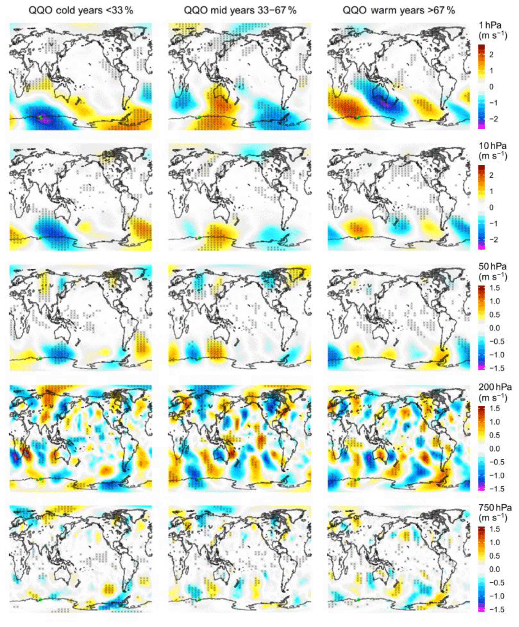
Figure 4Composites of the ERA5 (AMJJAS) meridional wind anomaly, for cold, mid, and warm years of the Davis detrended winter average QQO signal. Pressure levels are indicated on the right-hand colour bar. The colour scales are in metres per second. Hashed areas on the plots are significant at the 90 % level. Zonal wind anomaly equivalent in Fig. S3 (Supplement).
In Fig. 4, the 50, 10, and 1 hPa levels show large-scale patterns in mid- and high latitudes of the SH. For the cold-year composite, there is a region of negative (poleward) anomalous flow south of Australia towards Antarctica at 50 hPa that extends further poleward and westward towards and over Davis in the upper levels. At 1 hPa in the cold years, the pattern generally has a zonal wave-1 structure, which is also seen in the cold-year geopotential height anomaly composite at this level (top left panel of Fig. 3). The warm-year meridional wind composite (right panels of Fig. 4) appears to show a pattern that has a wave-2 structure in the upper levels, with a general orientation north-west to south-east at 1 hPa. In the region near Davis, the meridional wind anomaly is equatorward in the upper levels for the warm years. The intermediate years provide a contrast between the cold and warm years in the meridional wind, with regions that show an opposite sign in some of the regions common with either the cold- or warm-year composites. For example, at 1 hPa near Australia, the meridional wind anomaly is positive (equatorward) for the intermediate years and negative (poleward) for the warm years, whereas near the Antarctic Peninsula, the wind anomaly is positive in the cold years and negative in the intermediate years. The zonal wind composites (provided in Fig. S3) also show contrasting patterns between the cold-, intermediate-, and warm-year averages, particularly in the upper levels. Here regions of significant anomalies tend to extend into the tropics and NH. At 10 hPa the SH patterns tend to show a wave-2 structure in the cold and warm years.
Overall there are geographical regions showing some clear anti-phase relationships between the cold and warm years in the ERA5 composites (i.e. statistically significant and of opposite sign), but the intermediate years also show significant patterns suggesting that there may not be one clear driver for any association with the mesopause region temperatures. Some intermediate years are close to the cold or warm threshold, but varying the threshold did not significantly alter the patterns in the composites. We also produced composite maps using ERA5 temperatures (not shown). While able to span more years than possible with Aura/MLS temperatures, the ERA5 composites for the 1 and 10 hPa levels were qualitatively consistent with the correlation maps shown in the lower two rows of panels in Fig. 2b.
Figure 5 presents correlation maps of both the Davis OH residual winter average QQO signal (24 years; a) and Aura/MLS 0.0046 hPa polar cap (AMJJAS) residual QQO signal (14 years; b) against ERSST v5 anomalies (evaluated with respect to the 1995–2018 climatology). The strongest and most consistent patterns of anti-correlation (QQO warmest for below average SST) for the two epochs occur at mid-latitudes in the south-western Pacific Ocean (to the south of Australia and New Zealand; region marked D), in the south-western Atlantic Ocean (near the east coast of South America), and in the west-central Indian Ocean (to the west of Madagascar; region marked B). Significant positive correlation is also seen at mid-latitudes south of Africa (region marked A), and for the longer-term Davis data set, in the south-eastern Pacific Ocean. Time series of SST anomalies in regions A, B, C, and D are provided in Fig. S4. The correlation maps generally show a dipole-like pattern in the Indian Ocean (although the positive correlation in the east-central Indian Ocean is not significant) and weak or no correlation in the central Pacific Ocean, where ENSO SST anomalies tend to be located. Compared with the 500 hPa air temperature analysis of Pisoft et al. (2011), their Fig. 3 shows regions of high wavelet power in the QQO timescale at mid- and high southern latitudes for the ERA-40 reanalysis that bear some similarity to the location of regions of high correlation in Fig. 5a.
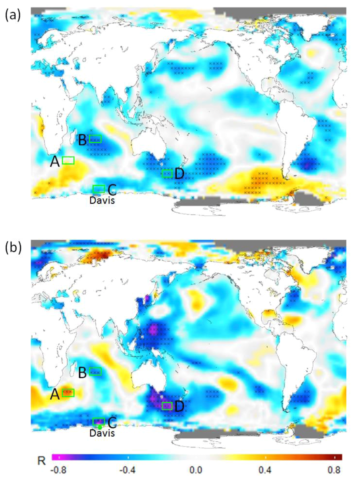
Figure 5Correlation maps of the Davis OH residual (24-year) QQO signal (a) and MLS 0.0046 hPa (AMJJAS) polar cap average residual (14-year) QQO signal (b) with the Extended Reconstructed Sea Surface Temperature (AMJJAS) average anomalies. Cross-hatched points are significant at the 90 % level (every second grid point marked). Grey areas are permanent sea ice.
4.1 QBO and ENSO relationships to the QQO
Residual variability in the Davis OH data set has been previously investigated by French and Klekociuk (2011) using indices for planetary wave activity (derived by zonal Fourier decomposition of the 10 hPa geopotential height at 67.5∘ S from the NCEP-DOE reanalysis, polar vortex intensity (PVI based on the zonal wind anomaly at 10 hPa), 30 hPa standardized QBO, and the Southern Annular Mode (SAM; calculated as the difference between the normalized monthly mean sea level pressure at 45 and 65∘ S). No statistically significant correlations were found with the PVI, QBO, or SAM indices over the entire data set (then extending 1995–2010); however, there was clear evidence of planetary wave modes identified in the 10 hPa NCEP reanalysis data penetrating to OH layer heights at different times in the series. Over the shorter time series, the QQO was not readily apparent in that study.
In a study of the SH summer mesosphere responses to ENSO, Li et al. (2016) suggest that constructive interference of ENSO and QBO could lead to stronger stratospheric westward zonal wind anomalies at SH high latitudes in November and December, thereby causing early breakdown of the SH stratospheric polar vortex during warm ENSO events in the westward phase of the QBO. This would in turn lead to greater SH mesospheric eastward gravity wave (GW) forcing and much colder mesospheric polar temperatures. The opposite effect would occur during cold ENSO events in the eastward QBO phase leading to warmer mesospheric polar temperatures. We have re-examined the QBO and ENSO indexes as likely candidates for a possible source of the observed QQO. However, comparing both 30 and 10 hPa Singapore QBO data (https://www.geo.fu-berlin.de/en/met/ag/strat/produkte/qbo/, last access: 3 July 2020) and the Multivariate ENSO index (MEIv2) (https://www.esrl.noaa.gov/psd/enso/mei/, last access: 3 July 2020) yields no significant correlation with the QQO variation. Time series plots are available in Figs. S5 and S6.
The clear presence of patterns in the ERA5 composite data in Fig. 3 (wave-1 structure at 1 hPa, in the cold years) and Fig. 4 (wave-2 structure at 1 hPa in the warm years) suggests that non-migrating tides or stationary planetary waves may have some part to play in the formation of the QQO. Baldwin et al. (2019) reported strong inter-annual variability in the amplitude of the diurnal migrating tide (DW1) observed in SABER temperature data, which appears to be related to the stratospheric QBO. Liu (2016) notes that the modulation of tides by the QBO and ENSO can have an impact at inter-annual timescales in a review of the influence of low atmosphere forcing on variability of the space environment. The absence of a direct correlation between the QQO and the QBO (or ENSO), together with the presence of distinctly different longitudinal wave patterns in the ERA5 geopotential and meridional wind anomalies during warm and cold years of the QQO, provide a tantalizing picture of the complexity of the mechanisms that influence the upper atmosphere.
4.2 Relationship with mesospheric zonal and meridional winds
To further explore the origin of the QQO temperature variation, we examined the AMJJAS mean meridional and zonal winds measured by the medium-frequency spaced antenna (MFSA) radar, co-located at Davis (Murphy et al., 2012). Correlations between the Davis OH and SABER residual temperatures (compared over the common satellite era 2002–2018) and the MFSA meridional wind at 86 km both yield R2 values of 0.51 as shown in Fig. 6. The Aura/MLS correlation R2 is 0.54 over the shorter time span (2005–2018). The correlation between mesopause region temperature and the meridional wind is such that higher (lower) temperatures correspond to poleward (equatorward) flow over the site. The regression coefficients are K (ms−1)−1 (Davis OH), K (ms−1)−1 (SABER), and K (ms−1)−1 (Aura/MLS). There is no significant correlation with the zonal wind.
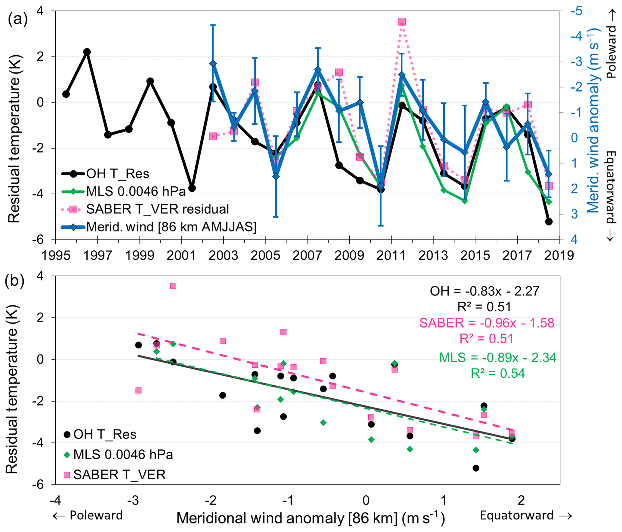
Figure 6(a) Davis OH, Aura/MLS (0.0046 hPa level) and SABER (T_VER) residual temperatures compared to the AMJJAS mean meridional wind at 86 km measured by MFSA radar at Davis. (b) The relationship between Davis OH, Aura/MLS, and SABER residual temperatures and meridional winds at 86 km above Davis. OH and SABER are fit over a common era (2002–2018) for comparison. MLS is fit over 2005–2018.
Garcia and Solomon (1985), Dyrland et al. (2010), and Espy et al. (2003) have reported a similar relation between temperature and the background meridional wind in the mesosphere. Espy et al. (2003) derive −0.71 K (ms−1)−1 R2=0.37 (Rothera 68∘ S, 62∘ W) and Dyrland et al. (2010) +0.51 K (ms−1)−1 R2=0.50 (Longyearbyen 78∘ N, 16∘ E; note opposite sign for poleward flow in NH). The relationship is explained in terms of adiabatic processes whereby poleward circulation leads to convergence and downwelling and therefore adiabatic heating, while equatorward circulation is symptomatic of upwelling and cooling. The correlation suggests that at least part of the temperature variation at Davis after the removal of the seasonal cycle, the solar cycle response, and the long-term linear trend is due to meridional circulation. This hypothesis is supported by the Aura/MLS polar cap correlation plots which show the highest correlation in the region of the SH polar cap, but only down to an altitude of ∼64 km (0.1 hPa).
4.3 CO as a tracer of vertical transport
Additional evidence supporting the association between temperature and large-scale adiabatic processes over the polar cap was obtained by examining the concentration of CO using Aura/MLS measurements. The primary source of CO in the upper stratosphere and mesosphere is photolysis of CO2, while production via oxidation of methane occurs throughout the middle atmosphere (Brasseur and Solomon, 2005; Lee et al., 2018). The long lifetime (>1 month) of CO makes it a useful tracer for vertical and meridional transport, particularly during the polar winter when there is a lack of photolysis over the polar cap. Figure 7 shows a general positive correlation between the time series of the SH polar cap winter residual temperature at 0.0046 hPa and CO mixing ratio at levels between 0.0046 and 0.1 hPa. Here we have used the same gridding and averaging as for Fig. 2 and obtain the residual by subtracting the seasonal cycle and a fitted solar cycle response for each grid box before forming averages over the polar cap. The linear correlation coefficient at 0.0046 hPa between the temperature and CO time series is 0.11, which increases to 0.43 (R2=0.18) on the removal of the linear trends from both time series (Temperature −0.74 K per decade and CO +0.65 ppmv per decade or % per decade). Detrended temperature sensitivity is then 0.73±0.45 K ppmv−1 CO. Similar values of R2 are observed down to the 10 hPa level on the removal of linear trends. The positive correlation is consistent with CO being transported into (out of) the polar cap by convergence (divergence) of air masses which cause adiabatic warming (cooling) in the process. As there is a strong positive vertical gradient in CO in the upper mesosphere (Lee et al., 2018), we suggest that the largest contribution to changes in CO in Fig. 7 is from vertical transport, rather than from horizontal transport. Below the 0.1 hPa pressure level, correlations diminish.

Figure 7Comparison of Aura/MLS SH polar cap (65–85∘ S) winter residual temperatures at 0.0046 hPa (green line; dashed linear fit −0.74 K per decade) with CO mixing ratio at 0.0046, 0.01, and 0.1 hPa (red line with dashed fit +0.65 ppmv per decade, orange line, and purple line respectively). Data are averaged over months AMJJAS and have had seasonal and solar cycle variations subtracted.
Figure 8 shows the spatial correlation between the polar cap QQO temperature signal at 0.0046 hPa and the CO residual mixing ratio at four pressure levels. In Fig. 8a, temperature and CO are significantly positively correlated over most of Antarctica, which is consistent with Fig. 7 and our hypothesis that the QQO temperature variation is an adiabatic response (i.e. increased (decreased) temperature is associated with increased (decreased) CO mixing ratio due to descent (ascent)). This general positive correlation over Antarctica is also seen for CO at 0.1 hPa (Fig. 8b) and is apparent though less clear for CO at 1 hPa (Fig. 8c). There are also regions of significant positive correlation with the south-east of Madagascar and near the southern tip of South America that are consistent with the regions of significant positive correlation in Fig. 2b. Note however that the region of significant negative correlation in Fig. 2b south of New Zealand also shows negative correlation in Fig. 8a, albeit mostly not significant. This suggests that temperature and CO mixing ratio are in opposing phases in this region, unlike the in-phase response over Antarctica. The implication here is that the response in the sub-New Zealand region does not tally with an adiabatic response. In the NH, there are generally no large-scale significant patterns of correlation. However it can be seen, particularly in Fig. 8a, that there are regions of significant correlation between the SH polar temperature and CO over northern mid-latitudes to high latitudes, which have negative correlation in Fig. 2b. This suggests that the QQO in the NH summer is in the opposite phase to the QQO in the SH winter, and that the forcing of temperature is consistent with an adiabatic response.
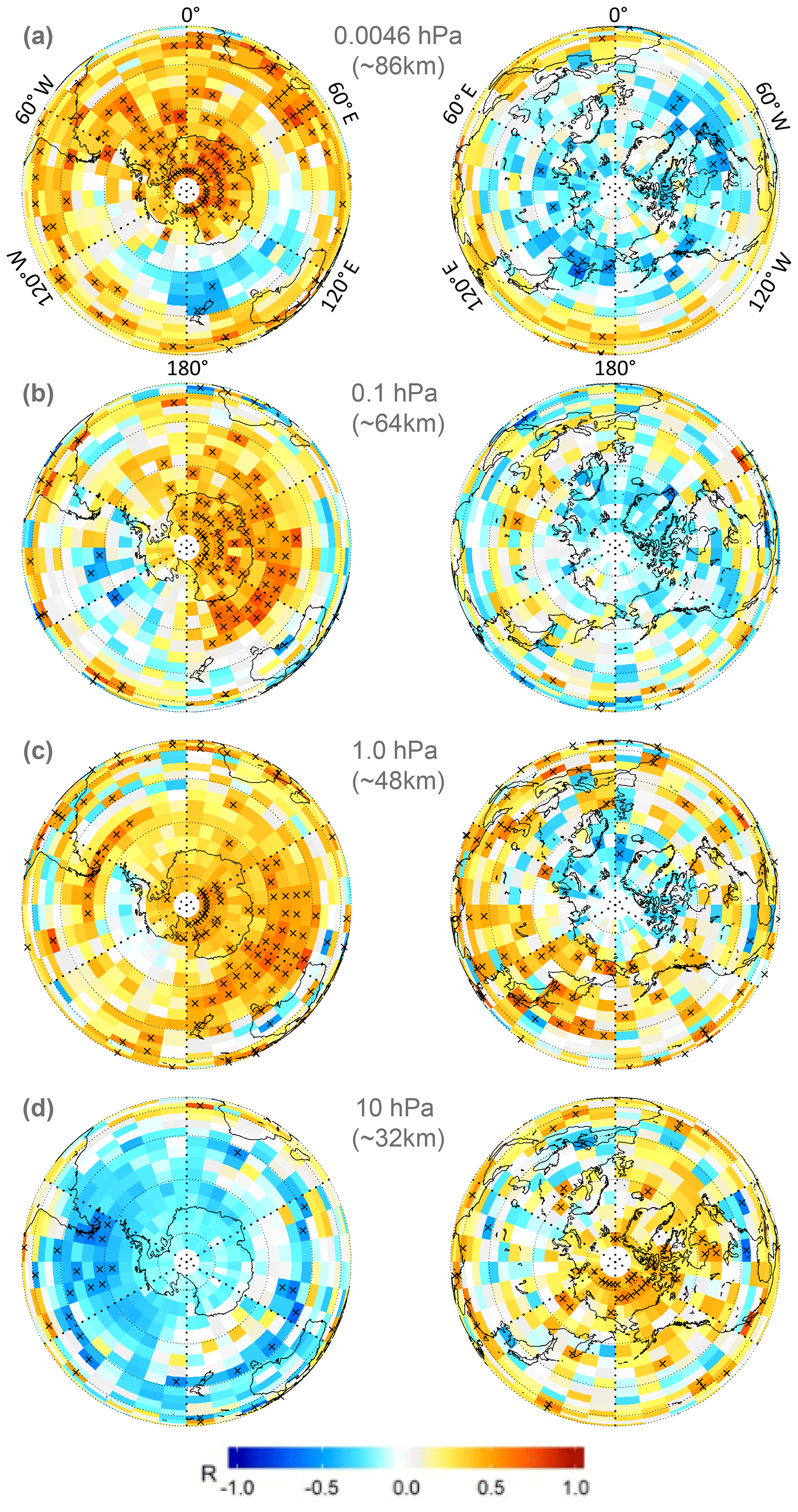
Figure 8SH and NH projection maps of correlation between the detrended Aura/MLS 0.0046 hPa, SH polar cap (65–85∘ S), and AMJJAS average temperature time series, with residual Aura/MLS CO mixing ratio in each grid box at the pressure levels indicated. Crosses indicate the correlation is significant at the 90 % level.
4.4 Relationship with SST and Antarctic sea ice
On the basis of the SST patterns apparent in Fig. 5, we examined the possibility of a response in Antarctic sea ice concentration from a QQO signal. We do not suggest that the upper mesosphere is responding to changes in sea ice but rather that both the upper mesosphere and sea ice may be responding to a common driver. Our motivation here was two-fold. Firstly, a near-surface QQO forcing might be expected to couple to sea ice through modification of oceanic and atmospheric heat flux and circulation (for example, promotion of sea ice formation due to cooling or surface divergence). Secondly, the Antarctic average sea ice extent since at least the 1990s has shown an indication of variability on a timescale of 4–6 years (e.g. Fig. 2c of Parkinson, 2019). We obtained the areal sea ice concentration from the NOAA Optimum Interpolation SST (OI-SST) data set version 2 (Reynolds et al., 2002). As can be seen in Fig. 9a, there are regions of significant negative correlation between the Davis OH residual temperature time series and OI-SST sea ice concentration towards the Antarctic coast between 30 and 60∘ E (south-east of Africa, region marked A ), and also centred on 120∘ W (in the Amundsen Sea, region marked B; ). The maximum anti-correlation is −0.61 at 61.5∘ S, 55.5∘ E (within region A, marked with a purple dot). These regions tend to lie to the south of regions where the SST is positively correlated with the Davis OH temperature residuals (Fig. 9b), consistent with warm (cold) SSTs reducing (increasing) sea ice concentration. A link between sea ice concentration and meridional and zonal wind could be expected if persistent near-surface circulation anomalies are related to the mesospheric QQO. For example, a persistent northward (southward) flow on one side of a circulation anomaly could increase (decrease) sea ice due to the associated flow of relatively cold (warm) air from higher (lower) latitudes and expansion (compaction) of the ice edge (e.g. Fig. 3 of Turner et al., 2016). Both the zonal and meridional near-surface (10 m) wind components (Fig. 9c and d) show regions of negative correlation with the Davis OH temperature QQO at the Antarctic coast near 30–60∘ E where the pattern in Fig. 9a is significant, but these correlations are generally weak and relatively small area. There are also regions of weak and not significant positive correlation around much of the equatorward edge of the sea ice zone.
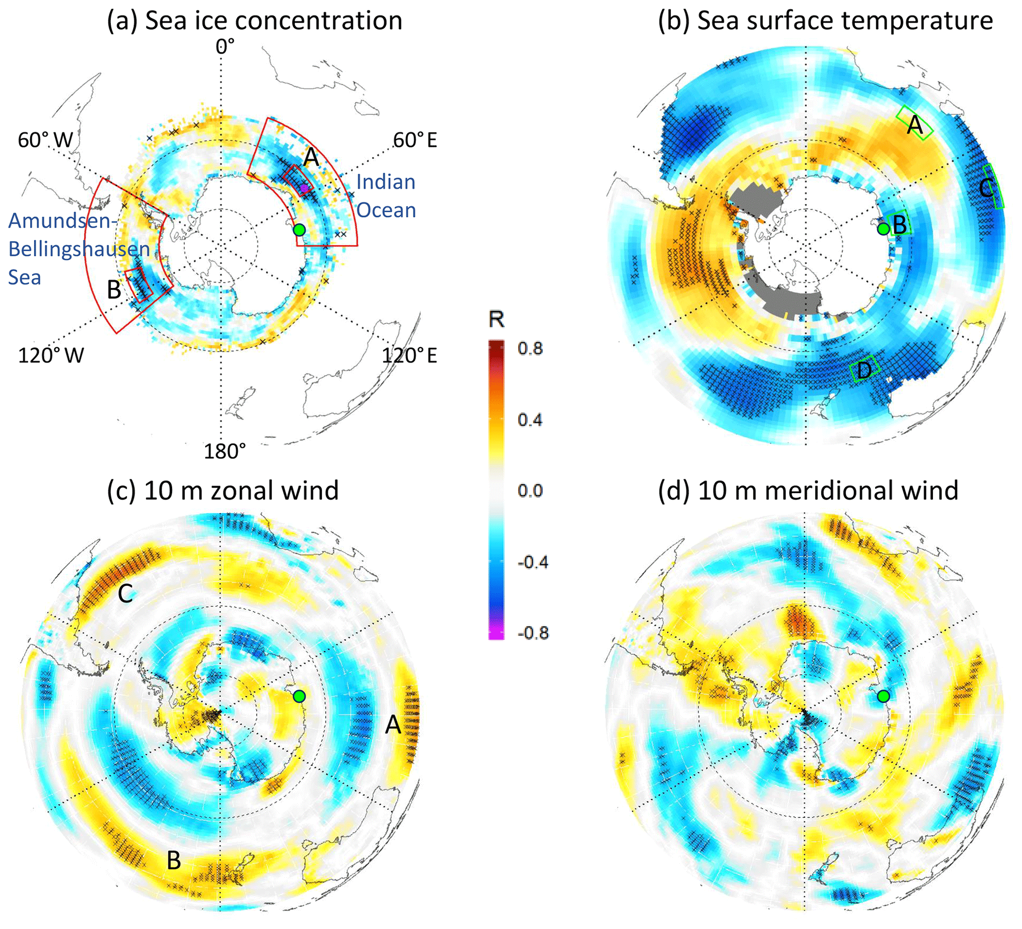
Figure 9Correlation maps of Davis OH 24-year QQO signal (green dot) with (a) sea ice concentration (OI-SST; Reynolds et al., 2002), (b) sea surface temperature (ERSSTv5), (c) surface (10 m) zonal wind anomaly (ERA5) and (d) surface (10 m) meridional wind anomaly (ERA5). Hashed areas are significant at the 90 % level.
Further equatorward from the Antarctic coast, Fig. 9c and d show correlation patterns (marked A, B, and C in Fig. 9c) that are suggestive of cyclonic (anticyclonic) circulation under warm (cold) QQO phases. These features appear to be consistent with the extent of negative (cyclonic) and positive (anti-cyclonic) geopotential height anomalies at 200 and 750 hPa in the warm and cold composites of Fig. 3 respectively (also marked A, B, and C in Fig. 3, bottom right panel). Intriguingly, the features appear close to the “gatekeeper” circulation features in the southern Indian Ocean (SIO), south-west Pacific Ocean (SWP), and south-west Atlantic Ocean (SWA) respectively, identified by Turney et al. (2015) as having a strong influence on Antarctic surface temperatures (see their Fig. 4). This could hint at the origin of the QQO forcing as residing with a tropical interaction with the mid- and high-latitude SH circulation, particularly in the wave-3 near-surface features of the southern high latitudes (Raphael, 2004), which potentially also influences surface conditions including sea ice. Furthermore, we note that Turney et al. (2015) in their Fig. 9 show periodicities in South Pole temperatures in the 4–6-year period in recent decades that appear to be associated with the variations in pressure in the SIO and SWP regions.
Figure 4c of Parkinson (2019) shows the annual time series of Antarctic sea ice extent in the Indian Ocean sector (20–90∘ E), which spans the general region of negative correlation at eastern longitudes in Fig. 9a (red box marked as “Indian Ocean”). While there is evidence for an anti-correlation of this sea ice time series with the Davis OH temperature residuals (Fig. S7; , R2=0.26, p=0.001), it is not consistent for all years (e.g. 1999). Parkinson (2019) also provides a sea ice time series for the Amundsen–Bellingshausen sea region (130–60∘ W; red box marked as “Amundsen–Bellingshausen Sea”), which covers part of the region of significant negative correlation in Fig. 9a (marked B) but also a more extensive region to the east towards the Antarctic Peninsula where the correlation is positive. For this region, there is an overall weak and not significant negative correlation between this specific time series and the Davis OH temperature residual (, R2=0.06, p=0.25).
Further investigation of sea ice variability in connection with a QQO signature is suggested, particularly as the annual time series of Antarctic sea ice extent presented in Fig. 2c of Parkinson (2019) appears to show 4–6-year variability, at least since the early 1990s, which generally appears anti-correlated with the QQO signal that we obtain for the upper mesosphere.
4.5 Hemispheric comparison
Returning to the phase response of the QQO signal between the hemispheres, we performed a similar analysis to that shown in Fig. 2 but using average temperatures (at the 0.0046 hPa pressure level) across the Arctic polar cap (65–85∘ N) in winter months (October to March, ONDJFM) and summer months (AMJJAS). We compare the time series in Fig. 10, together with SH polar cap winter (green line with linear fit) and summer (purple line) time series. First, we see little evidence of a QQO variation in the NH winter (blue line with linear fit), suggesting that the mechanism that drives the QQO in the SH winter is not as strong, or absent, in the NH winter. In summer the SH response is generally in-phase with the SH winter, except in the years 2005–2008 but of considerably greater amplitude than the winter season. For the NH summer (orange line), a QQO response is apparent with a similar amplitude to the SH summer but an approximately opposite phase to the SH (except for the years 2005–2006). Our QQO signal for the NH summer polar cap shown in Fig. 10 is consistent with temperatures for 2002–2010 NH summers shown in Fig. 5 of Russell et al. (2014) poleward of 60∘ N using TIMED/SABER and Aura/MLS data.
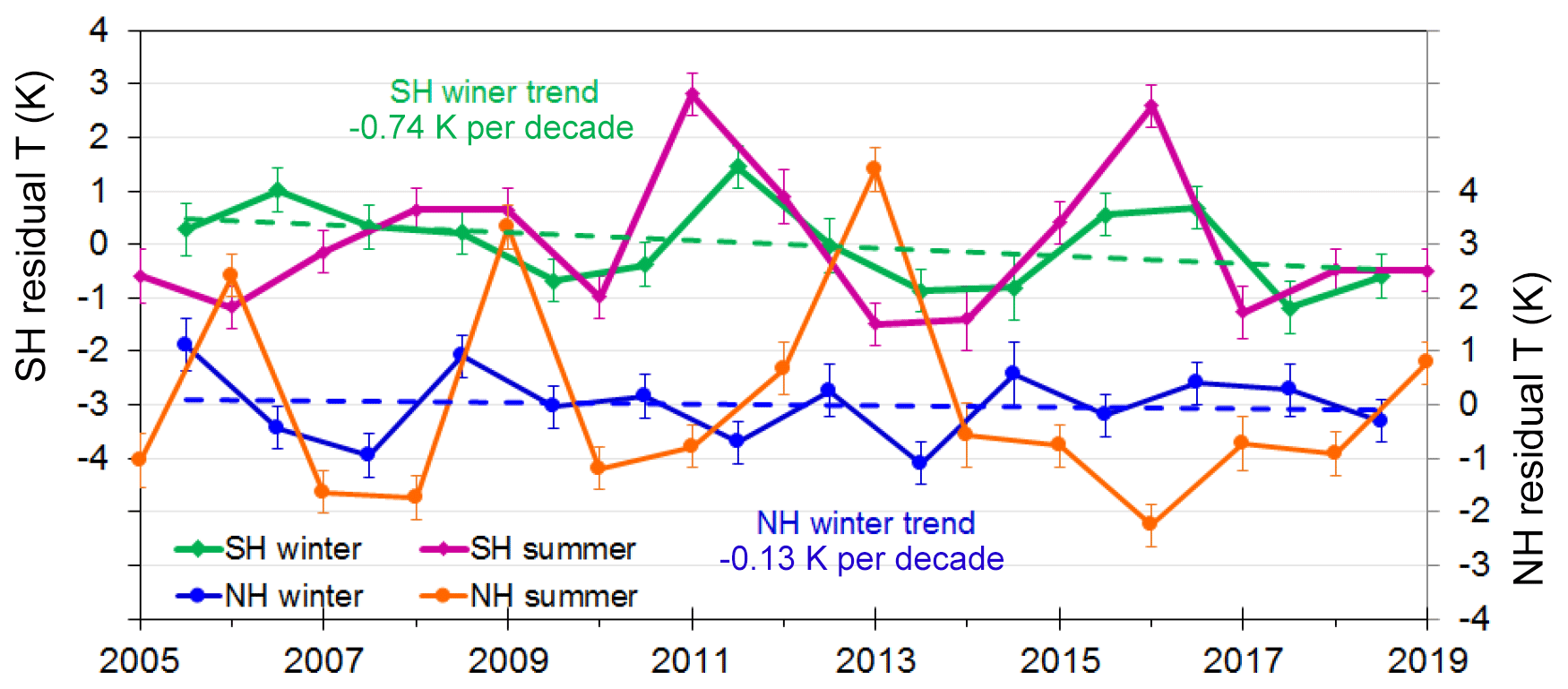
Figure 10Time series of Aura/MLS temperature residuals at the 0.0046 hPa pressure level averaged over the SH polar cap (65–85∘ S) for winter months (AMJJAS; light green line) and summer months (ONDJFM; purple line) and the NH polar cap (65–85∘ N) for summer months (AMJJAS; orange line) and winter months (ONDJFM; blue line). Scales offset by 3 K for clarity.
4.6 Comparison with CESM-WACCM
Following on from Offermann et al. (2015), we examined simulations produced from a version of CESM-WACCM for phase 1 of the Chemistry-Climate Model Initiative (CCMI-1; Morgenstern et al., 2017), specifically the CESM1 WACCM model which includes both interactive atmospheric chemistry and interactive ocean physics to provide a self-consistent simulation of climate. Our interest here is to see if the model physics produces a QQO response in the mesosphere, particularly as Offermann et al. (2015) had noted that the CESM-WACCM model showed low-frequency variability in temperatures on 3–6-year timescales over central Europe. We obtained three ensemble members from the REF-C2 simulation of the model spanning 1955–2100. The REF-C2 simulation follows particular scenarios for interactive chemistry involving ozone-depleting substances and radiative forcing (the WMO A1 and RCP 6.0 scenarios respectively; Morgenstern et al., 2017), with a repeating synthetic solar cycle beyond 2010. SH polar cap (65–85∘ S) temperatures were averaged over AMJJAS for pressure levels of 0.01 Pa (∼105 km altitude), 0.5 Pa (∼85 km), and 0.15 hPa (∼60 km), and Morlet wavelet analysis (Torrence and Compo, 1998) was applied to the individual ensemble members. While a solar-cycle (10–11-year period) signal was detected with better than 95 % confidence for all ensemble members near and above the 0.01 hPa level, no periodicity in the 3–6-year range exceeded the 95 % confidence limit in the mean spectrum for any member. We do note, however, that particular ensemble members showed power that was significant at the 95 % confidence limit in the 2–3-year period range in certain epochs (Fig. S8) and in some cases in the 4–5-year period range. We therefore cannot rule out that the model does not reproduce the QQO signal, but the significance and amplitude of any signal over recent decades of the historical period in the Antarctic mesopause region appears to be less than in our observations.
4.7 Gravity wave interactions
We now consider why our SH winter QQO signal appears generally restricted to the mesosphere. It is well known that the Antarctic Peninsula is a hot spot for gravity wave activity at the edge of the southern polar cap (Hoffmann et al., 2013) and this region is consistently active during austral autumn, winter, and spring. Many GWs are able to penetrate all the way up to the mesosphere before their amplitudes become so large that they break and deposit their energy, thereby introducing perturbations in winds and temperatures. Correlation coefficients below the 0.1 hPa level (∼65 km) in our Aura/MLS analysis are potentially low because few GWs break below this altitude. The strong eastward stratospheric winds of the polar night jet filter out many eastward-propagating GWs creating a westward drag on winds in the mesosphere, which, when combined with the Coriolis force, generates a weak poleward flow. This flow is modulated by inter-annual variations in upward propagation of GWs and agrees with the view of Solomon et al. (2018), who attribute the significant inter-annual variability of mesopause temperatures to the dominance of dynamical processes in their control. Further support for this view can be found in Sato et al. (2012), who employed a high-resolution middle atmosphere general circulation model (GCM) to examine gravity wave propagation in the middle to high latitudes of the SH without the need for gravity wave parameterization. Gravity wave energy is generally weak in summer, but in winter, gravity waves have large amplitudes and are distributed around the polar vortex in the upper stratosphere and mesosphere. The wave energy is not zonally uniformly distributed but is concentrated on the leeward side of the Southern Andes and Antarctic Peninsula. Energy propagation extends several thousand kilometres eastwards, which explains the gravity wave distribution around the polar vortex in winter.
Examining the Aura/MLS polar cap correlation plots in Fig. 2b and c in detail, we see that maps of GW potential energy (PE) at 10 hPa calculated for the winter months by Sato et al. (2012; their Fig. 2) are well reproduced at 0.01 hPa and higher altitudes and that the region of the highest correlation becomes more concentrated as GWs are filtered out with increasing altitude. It is also likely that GWs are strongly focused into the polar night wind jet (Wright et al., 2017). Wright et al. (2016) reported strong correlations between GW potential energy and vertical wavelength with stratospheric winds but not local surface winds from a multi-instrument gravity wave investigation over Tierra del Fuego and the Drake Passage. The results of Sato et al. (2012), together with the focusing of GWs into the polar night wind reported by Wright et al. (2016, 2017) suggest GWs as a plausible explanation for the asymmetry in the polar projection plots of the QQO correlation coefficient at 0.01 hPa and above.
4.8 Mechanisms for a 4-year cycle
The question remains as to why this modulation has a quasi 4-year cycle. Zhang et al. (2017) detected both 3- and 4-year oscillations in zonal mean SABER temperatures at 85 km altitude in the period 2002–2015 using Lomb–Scargle analysis, in which the much stronger annual, semi-annual, quasi-biennial, and 11-year periods were also present. The latitude range studied was limited to 50∘ S–50∘ N because of the satellite yaw cycle; the 4-year oscillation was found to have a stronger peak in the SH. Although the origin of the 4-year oscillation is not discussed in Zhang et al. (2017), it is suggested that the 3-year oscillation is a sub-peak of the QBO and is due to modulation of the QBO possibly by the semi-annual oscillation. Their analysed SABER temperatures also show evidence of the 4-year oscillation at 25 km altitude, but not at 45 km. We note that a QQO variability observed in Jupiter's equatorial winds has been inferred to result from forcing by gravity waves produced by deep convection (Cosentino et al., 2017).
Liu et al. (2017) examined variations in global gravity waves from 14 years of SABER temperatures between 2002 and 2015. Unfortunately, their study was also limited to the latitude band 50∘ S–50∘ N because of the TIMED 60 d yaw cycle. They applied multivariate linear regression to calculate trends of global GW potential energy and the responses of GW PE to solar activity, to the QBO, and to ENSO. They found a positive trend in GW PE with a maximum of 12 %–15 % per decade at 40–50∘ S below 60 km altitude. This was interpreted as a possible indication of eddy diffusion increase in some locations and at 50∘ S could be due to a strengthening of the polar stratospheric jets. The global gravity wave response to solar activity is negative in lower and mid-latitudes in the mesosphere–lower-thermosphere (MLT) region. It is also negative to the QBO eastward wind phase in the tropics and is more negative in the NH than in the SH MLT region. The response of global GWs to the ENSO index is positive in the tropical stratosphere (Geller et al., 2016).
Yasui et al. (2016) examined the seasonal and inter-annual variations in GWs (50–100 km) using an MF radar at Syowa station (1999–2013). They found that the Antarctic summer inter-annual modulation could not be explained by the proposed mechanism of sudden stratospheric warmings in the Arctic via inter-hemisphere coupling. Two other proposed mechanisms were found to be the more likely origin of the modulation; these were (a) the modulation of the vertical filtering of GWs in association with breakdown of the polar vortex in the SH and (b) tropical convection and propagation to the Antarctic region. Two of the periods noted in the Introduction in the study of the mesosphere over central Europe reported by Offermann et al. (2015) (3.4 and 5.5 years) fit well with the correlation results for Aura/MLS temperatures at different pressure levels in Fig. 2 of the present study. The amplitude of the oscillations they report (∼1 K) is about half those observed in the QQO at Davis. Offermann et al. (2015) suggest harmonics of the 11-year solar cycle at 5.5, 3.6, and 2.2 years as possible origins of these oscillations. In addition, Offermann et al. (2015) state that oscillations with similar periods are found in the GLOTI (Global Land Ocean Temperature Index) and NAO (North Atlantic Oscillation index) data. This is an interesting observation in the context of the correlation maps of the Davis QQO signal with Extended Reconstructed Sea Surface Temperature shown in Fig. 5.
The variability in winter temperatures derived from hydroxyl airglow observations at Davis station is examined after seasonal, solar cycle, and long-term linear trend terms are removed (in Part 1 of this work, French et al., 2020). The following observations are made regarding this variability:
-
A strong QQO feature (3–4 K peak-to-peak amplitude, 3.5–4.5-year period) has been observed in the mesopause region winter average temperatures measured at Davis research station, which has been sustained over more than two solar cycles (24 years).
-
Previous reports of QQO signals have tended to be associated with the ENSO phenomenon and sea surface temperatures or the wind field over equatorial regions, but this is the first report of its presence at high-latitude mesopause altitudes.
-
Hydroxyl-layer equivalent winter average (AMJJAS) temperatures from both Aura/MLS (from 2005) and TIMED/SABER (from 2002) in the vicinity of the station (within 500 km) agree well with the Davis OH temperature QQO in amplitude, period, and phase.
-
The Davis QQO pattern shows a significant positive correlation with the Aura/MLS 0.0046 hPa temperature field over a large part of the Antarctic polar cap and southern Indian Ocean sectors and significant anti-correlation in the Southern Ocean below New Zealand. The polar cap winter average (AMJJAS; 65–85∘ S) has a very similar QQO pattern to the Davis site revealing that the feature has a large spatial scale.
-
There is a general region of negative correlation at mid-latitudes to high latitudes, in the NH summer, indicating that the QQO has opposite phases in the two hemispheres.
-
Correlation of the SH polar cap average QQO signal shows that the pattern extends vertically at least from the mesopause region (∼86 km) down to 0.1 hPa (∼64 km) and then becomes anti-correlated in the upper stratosphere (1–10 hPa). Again, this pattern is opposite in the NH.
-
Composite analysis with ERA5 geopotential height anomaly indicates that warm years of the QQO are associated with higher than average geopotential height anomalies over the polar cap, the East Antarctic sector of the Southern Ocean (sub-Africa), and the Amundsen Sea region and lower than average anomalies in the southern Pacific, Indian, and Atlantic regions. Cold years are associated with the opposite and the effect is greater at higher altitudes (10 and 1 hPa levels). There is the indication of a connection with persistent near-surface circulation anomalies in the southern Indian Ocean and south-west Pacific Ocean and variability in Antarctic sea ice.
-
Composite analysis with ERA5 data also indicates the presence of distinctly different wave patterns in the ERA5 geopotential and meridional wind anomalies during the warm and cold years of the QQO, indicative of a potential role of planetary waves or atmospheric tides in the QQO.
-
Correlation with the meridional wind anomaly at 86 km measured by the Davis medium-frequency spaced antenna radar shows that about 51 % of the mesopause temperature QQO can be explained by the adiabatic cooling (heating) resulting from meridional circulation. This result is supported by the correlation between temperature and Aura/MLS CO measurements on a global scale as reported by Lee et al. (2018). Modulation of the meridional circulation is possibly a result of the variation in gravity wave filtering by the strong stratospheric winds during the polar night.
Taken together, these points highlight the interconnectedness of the entire atmosphere–ocean system and that the QQO may be a manifestation of some type of normal oscillatory atmospheric mode arising from atmosphere–ocean interactions. Our efforts to isolate a specific mechanism that would drive a QQO, such as combinations of ENSO, QBO, PVI, and SAM (like those proposed by Li et al. (2016) in the SH summer) have not found anything definite in the winter data at this time, and further investigations are warranted.
As we have shown, the QQO signal is also present in the polar summer mesosphere, and consequently there are implications for multi-year variability in the summer polar phenomena of noctilucent clouds (or polar mesospheric clouds, PMCs) and polar mesospheric summer echoes. It would be expected that the temperature perturbations of 3–4 K that accompany the QQO at the mesopause will tend to have the most significant influence where temperatures hover near the ice–aerosol formation threshold, perturbed by gravity waves, planetary waves, and tides. Indeed, the QQO signal may explain part of the variability in the position of the low-latitude boundary and modelled occurrence of noctilucent clouds in the NH reported by Russell et al. (2014) and the albedo of PMC for the SH and NH reported by Liu et al. (2016). The implications of the QQO for long-term trends in these mesospheric phenomena deserve further study.
All Davis hydroxyl rotational data described in this paper are available through the Australian Antarctic Data Centre website (under project AAS4157) via the following link – https://data.aad.gov.au/metadata/records/Davis_OH_airglow (Burns and French, 2002), last access: 11 June 2020. The satellite data used in this paper were obtained from the Aura/MLS archive at the Goddard Earth Sciences (GES) Data and Information Services Center Distributed Active Archive Center (DAAC) (see https://disc.gsfc.nasa.gov/datasets/ML2T_004/summary?keywords=MLS, Schwartz et al., 2008, last access: 3 July 2020 and https://mls.jpl.nasa.gov/index-eos-mls.php, Schwartz et al., 2008, last access: 3 July 2020) and the SABER data archive (see http://saber.gats-inc.com/data.php, Russell III et al., 1999, last access: 3 July 2020) and are publicly available. The ECMWF/ERA5 reanalysis data are publicly available from the Copernicus Climate Data Store (https://cds.climate.copernicus.eu/cdsapp#!/dataset/reanalysis-era5-pressure-levels-monthly-means?tab=overview, Copernicus Climate Change Service (C3S), 2017, last access: 3 July 2020). ERSST and OI-SST data sets are publicly available from the NOAA Physical Science Division website (https://psl.noaa.gov/data/gridded/data.noaa.ersst.v4.html, Huang et al., 2014, last access: 3 July 2020 and https://psl.noaa.gov/data/gridded/data.noaa.oisst.v2.html, Reynolds et al., 2002, last access: 3 July 2020) and were accessed via the KNMI Climate Explorer site (https://climexp.knmi.nl/, Trouet and Van Oldenborgh, 2013, last access: 3 July 2020). CESM-WACCM data were obtained from the British Atmospheric Data Center (https://catalogue.ceda.ac.uk/uuid/1d9825e2b05b48cdb7971ced8c63965a, Morgenstern et al., 2017, last access: 3 July 2020).
The supplement related to this article is available online at: https://doi.org/10.5194/acp-20-8691-2020-supplement.
WJRF managed data collection, performed data analysis, and prepared the paper and figures with contributions from all co-authors. ARK analysed Aura/MLS satellite data and provided interpretation and paper and figure editing. FJM analysed SABER data and provided interpretation and editing of the paper, figures, and references.
The authors declare that they have no conflict of interest.
The authors thank the dedicated work of the Davis optical physicists and engineers over many years in the collection of airglow data and calibration of instruments. We thank Damian Murphy for provision of the MFSA radar data from Davis. These projects are supported by the Australian Antarctic Science Program (projects AAS 4157 and AAS 4025). We thank both the Aura/MLS and TIMED/SABER science teams for the use of the global satellite data as described in the “Data availability” section.
We acknowledge and thank the science teams behind the reanalysis data ERA5, ERSST, OI-SST, and the CESM-WACCM model as described in the “Data availability” section for the use of these data sets.
We acknowledge the efforts of the Network for Detection of Mesospheric Change (https://ndmc.dlr.de/, last access: 3 July 2020) in coordinating research to understand mesospheric change processes.
This work is undertaken within the Australian Antarctic Science Program (projects AAS 4157 and AAS 4025) under the Australian Government Department of Agriculture, Water and the Environment.
This paper was edited by Franz-Josef Lübken and reviewed by two anonymous referees.
Baldwin, M. P., Birner, T., Brasseur, G., Burrows, J., Butchart, N., Garcia, R., Geller, M., Gray, L., Hamilton, K., Harnik, N., Hegglin, M. I., Langematz, U., Robock, A., Sato, K., and Scaife, A.: 100 Years of Progress in Understanding the Stratosphere and Mesosphere, Meteorol. Monogr., 59, 27.1–27.62, https://doi.org/10.1175/amsmonographs-d-19-0003.1, 2019.
Brasseur, G. and Solomon, S.: Aeronomy of the Middle Atmosphere: Chemistry and Physics of the Stratosphere and Mesosphere, Springer Nature, Dordrecht, the Netherlands, https://doi.org/10.1007/1-4020-3824-0, 2005.
Burns, G. and French, J.: Rotational temperature studies of the hydroxyl airglow layer above Davis, Antarctica, Ver. 8, Australian Antarctic Data Centre – https://data.aad.gov.au/metadata/records/Davis_OH_airglow (last access: 3 July 2020), 2002.
Copernicus Climate Change Service (C3S): ERA5: Fifth generation of ECMWF atmospheric reanalyses of the global climate, Copernicus Climate Change Service Climate Data Store (CDS), available at: https://cds.climate.copernicus.eu/cdsapp#!/home (last access: 3 July 2020), 2017.
Cosentino, R. G., Morales-Juberías, R., Greathouse, T., Orton, G., Johnson, P., Fletcher, L. N., and Simon, A.: New Observations and Modeling of Jupiter's Quasi-Quadrennial Oscillation, J. Geophys. Res.-Planet., 122, 2719–2744, https://doi.org/10.1002/2017JE005342, 2017.
Dyrland, M. E., Mulligan, F. J., Hall, C. M., Sigernes, F., Tsutsumi, M., and Deehr, C. S.: Response of OH airglow temperatures to neutral air dynamics at 78∘ N, 16∘ E during the anomalous 2003–2004 winter, J. Geophys. Res., 115, D07103, https://doi.org/10.1029/2009JD012726, 2010.
Espy, P. J., Hibbins, R. E., Jones, G. O. L., Riggin, D. M., and Fritts, D. C.: Rapid, large-scale temperature changes in the polar mesosphere and their relationship to meridional flows, Geophys. Res. Lett., 30, 44.1–44.4, https://doi.org/10.1029/2002GL016452, 2003.
French, W. J. R. and Klekociuk, A. R.: Long-term trends in Antarctic winter hydroxyl temperatures, J. Geophys. Res., 116, D00P09, https://doi.org/10.1029/2011JD015731, 2011.
French, W. J. R. and Mulligan, F. J.: Stability of temperatures from TIMED/SABER v1.07 (2002–2009) and Aura/MLS v2.2 (2004–2009) compared with OH(6–2) temperatures observed at Davis Station, Antarctica, Atmos. Chem. Phys., 10, 11439–11446, https://doi.org/10.5194/acp-10-11439-2010, 2010.
French, W. J. R., Mulligan, F. J., and Klekociuk, A. R.: Analysis of 24 years of mesopause region OH rotational temperature observations at Davis, Antarctica – Part 1: long-term trends, Atmos. Chem. Phys., 20, 6379–6394, https://doi.org/10.5194/acp-20-6379-2020, 2020.
Garcia, R. R. and Solomon, S.: The effect of breaking gravity waves on the dynamics and chemical composition of the mesosphere and lower thermosphere, J. Geophys. Res., 90, 3850–3868, https://doi.org/10.1029/JD090iD02p03850, 1985.
García-Comas, M., López-Puertas, M., Marshall, B. T., Wintersteiner, P. P., Funke, B., Bermejo-Pantaleón, D., Mertens, C. J., Remsberg, E. E., Gordley, L. L., Mlynczak, M. G., and Russell III, J. M.: Errors in Sounding of the Atmosphere using Broadband Emission Radiometry (SABER) kinetic temperature caused by non-local-thermodynamic-equilibrium model parameters, J. Geophys. Res., 113, D24106, https://doi.org/10.1029/2008JD010105, 2008.
Geller, M. A., Zhou, T., Shindell, D., Ruedy, R., Aleinov, I., Nazarenko, L., Tausnev, N. L., Kelley, M., Sun, S., Cheng, Y., Field, R. D., and Faluvegi, G.: Modeling the QBO-Improvements resulting from higher-model vertical resolution, J. Adv. Model. Earth Syst., 8, 1092–1105, https://doi.org/10.1002/2016MS000699, 2016.
Hoffmann, L., Xue, X., and Alexander, M. J.: A global view of stratospheric gravity wave hotspots located with Atmospheric Infrared Sounder observations, J. Geophys. Res.-Atmos., 118, 416–434, https://doi.org/10.1029/2012JD018658, 2013.
Huang, B., Thorne, P. W., Banzon, V. F., Boyer, T., Chepurin, G., Lawrimore, J. H., Menne, M. J., Smith, T. M., Vose, R. S., and Zhang, H.-M.: Extended Reconstructed Sea Surface Temperature, Version 5 (ERSSTv5): Upgrades, Validations, and Intercomparisons, J. Clim., 30, 8179–8205, https://doi.org/10.1175/JCLI-D-16-0836.1, 2017.
Jiang, N., Neelin, J. D., and Ghil, M.: Quasi-quadrennial and quasi-biennial variability in the equatorial Pacific, Clim. Dynam., 12, 101–112, https://doi.org/10.1007/BF00223723, 1995.
Langhoff, S. R., Werner, H. J., and Rosmus, P.: Theoretical Transition Probabilities for the OH Meinel System, J. Mol. Spectrosc., 118, 507–529, 1986.
Lee, J. N., Wu, D. L., Ruzmaikin, A., and Fontenla, J.: Solar cycle variations in mesospheric carbon monoxide, J. Atmos. Sol.-Terr. Phys., 170, 21–34, https://doi.org/10.1016/j.jastp.2018.02.001, 2018.
Li, T., Calvo, N., Yue, J., Russell, J. M., Smith, A. K., Mlynczak, M. G., Chandran, A., Dou, X., Liu, A. Z., Li, T., Calvo, N., Yue, J., III, J. M. R., Smith, A. K., Mlynczak, M. G., Chandran, A., Dou, X., and Liu, A. Z.: Southern Hemisphere Summer Mesopause Responses to El Niño–Southern Oscillation, J. Clim., 29, 6319–6328, https://doi.org/10.1175/JCLI-D-15-0816.1, 2016.
Liu, C. and Xue, F.: The relationship between the canonical ENSO and the phase transition of the Antarctic oscillation at the quasi-quadrennial timescale, Acta Oceanol. Sin., 29, 26–34, https://doi.org/10.1007/s13131-010-0073-4, 2010.
Liu, H.-L.: Variability and predictability of the space environment as related to lower atmosphere forcing, Space Weather, 14, 634–658, https://doi.org/10.1002/2016SW001450, 2016.
Liu, S. and Duan, A.: Impacts of the global sea surface temperature anomaly on the evolution of circulation and precipitation in East Asia on a quasi-quadrennial cycle, Clim. Dynam., 51, 4077–4094, https://doi.org/10.1007/s00382-017-3663-4, 2018.
Liu, X., Yue, J., Xu, J., Yuan, W., Russell, J. M., Hervig, M. E., and Nakamura, T.: Persistent longitudinal variations in 8 years of CIPS/AIM polar mesospheric clouds, J. Geophys. Res.-Atmos., 121, 8390–8409, https://doi.org/10.1002/2015JD024624, 2016.
Liu, X., Yue, J., Xu, J., Garcia, R. R., Russell, J. M., Mlynczak, M., Wu, D. L., and Nakamura, T.: Variations of global gravity waves derived from 14 years of SABER temperature observations, J. Geophys. Res.-Atmos., 122, 6231–6249, https://doi.org/10.1002/2017JD026604, 2017.
Livesey, N. J., Read, W. G., Wagner, P. A.. Froidevaux, L., Lambert, A., Manney, G. L., Millán Valle, L. F., Pumphrey, H. C., Santee, M. L., Schwartz, M. J., Wang, S., Fuller, R. A., Jarnot, R. F., Knosp, B. W., Martinez, E., and Lay, R. R.: Earth Observing System (EOS) Aura Microwave Limb Sounder (MLS) Version 4.2x Level 2 and 3 data quality and description document, Version 4.2x-4.0, 1-168, JPL D-33509 Rev. E, available at: https://mls.jpl.nasa.gov/data/v4-2_data_quality_document.pdf, last access: 3 July 2020.
Marsh, D. R., Mills, M. J., Kinnison, D. E., Lamarque, J.-F., Calvo, N., and Polvani, L. M.: Climate Change from 1850 to 2005 Simulated in CESM1(WACCM), J. Clim., 26, 7372–7391, https://doi.org/10.1175/JCLI-D-12-00558.1, 2013.
McDade, I. C.: The altitude dependence of the OH(X2Π) vibrational distribution in the nightglow: Some model expectations, Planet. Space Sci., 39, 1049–1057, https://doi.org/10.1016/0032-0633(91)90112-N, 1991.
Mertens, C. J., Mlynczak, M. G., Lopez-Puertas, M., Wintersteiner, P. P., Picard, R. H., Winick, J. R., Gordley, L. L., and Russell III, J. M.: Retrieval of kinetic temperature and carbon dioxide abundance from nonlocal thermodynamic equilibrium limb emission measurements made by the SABER experiment on the TIMED satellite, in: Remote Sensing of Clouds and the Atmosphere VII, SPIE, Vol. 4882, p. 162, 2003.
Morgenstern, O., Hegglin, M., Rozanov, E., O'Connor, F., Luke Abraham, N., Akiyoshi, H., Archibald, A., Bekki, S., Butchart, N., Chipperfield, M., Deushi, M., Dhomse, S., Garcia, R., Hardiman, S., Horowitz, L., Jöckel, P., Josse, B., Kinnison, D., Lin, M., Mancini, E., Manyin, M., Marchand, M., Marécal, V., Michou, M., Oman, L., Pitari, G., Plummer, D., Revell, L., Saint-Martin, D., Schofield, R., Stenke, A., Stone, K., Sudo, K., Tanaka, T., Tilmes, S., Yamashita, Y., Yoshida, K., and Zeng, G.: Review of the global models used within phase 1 of the Chemistry-Climate Model Initiative (CCMI), Geosci. Model Dev., 10, 639–671, https://doi.org/10.5194/gmd-10-639-2017, 2017.
Murphy, D. J., Alexander, S. P., and Vincent, R. A.: Interhemispheric dynamical coupling to the southern mesosphere and lower thermosphere, J. Geophys. Res.-Atmos., 117, D08114, https://doi.org/10.1029/2011JD016865, 2012.
Offermann, D., Goussev, O., Kalicinsky, C., Koppmann, R., Matthes, K., Schmidt, H., Steinbrecht, W., and Wintel, J.: A case study of multi-annual temperature oscillations in the atmosphere: Middle Europe, J. Atmos. Sol.-Terr. Phys., 135, 1–11, https://doi.org/10.1016/j.jastp.2015.10.003, 2015.
Parkinson, C. L.: A 40-y record reveals gradual Antarctic sea ice increases followed by decreases at rates far exceeding the rates seen in the Arctic, P. Natl. Acad. Sci. USA, 116, 14414–14423, https://doi.org/10.1073/pnas.1906556116, 2019
Perminov, V. I., Semenov, A. I., Pertsev, N. N., Medvedeva, I. V., Dalin, P. A., and Sukhodoev, V. A.: Multi-year behaviour of the midnight OH∗ temperature according to observations at Zvenigorod over 2000–2016, Adv. Sp. Res., 61, 1901–1908, https://doi.org/10.1016/J.ASR.2017.07.020, 2018.
Pisoft, P., Miksovsky, J., Kalvova, J., Raidl, A., and Zak, M.: Areal analysis of oscillations in 500-hPa temperature field: a pseudo-2D wavelet transform approach, Int. J. Climatol., 31, 1545–1553, https://doi.org/10.1002/joc.2167, 2011.
Raphael, M. N.: A zonal wave 3 index for the Southern Hemisphere, Geophys. Res. Lett., 31, L23212, https://doi.org/10.1029/2004GL020365, 2004.
Reid, I. M., Spargo, A. J., and Woithe, J. M.: Seasonal variations of the nighttime O(1S) and OH(8–3) airglow intensity at Adelaide, Australia, J. Geophys. Res.-Atmos., 119, 6991–7013, https://doi.org/10.1002/2013JD020906, 2014.
Reynolds, R. W., Rayner, N. A., Smith, T. M., Stokes, D. C., and Wang, W.: An Improved In Situ and Satellite SST Analysis for Climate, J. Clim., 15, 1609–1625, https://doi.org/10.1175/1520-0442(2002)015<1609:AIISAS>2.0.CO;2, 2002.
Russell III, J. M., Mlynczak, M. G., Gordley, L. L., Tansock, J., and Esplin, R.: An Overview of the SABER Experiment and Preliminary Calibration Results, SPIE Proc., 3756, 277–288, https://doi.org/10.1117/12.366382, 1999.
Russell, J. M., Rong, P., Hervig, M. E., Siskind, D. E., Stevens, M. H., Bailey, S. M., and Gumbel, J.: Analysis of northern midlatitude noctilucent cloud occurrences using satellite data and modeling, J. Geophys. Res.-Atmos., 119, 3238–3250, https://doi.org/10.1002/2013JD021017, 2014.
Sato, K., Tateno, S., Watanabe, S., Kawatani, Y., Sato, K., Tateno, S., Watanabe, S., and Kawatani, Y.: Gravity Wave Characteristics in the Southern Hemisphere Revealed by a High-Resolution Middle-Atmosphere General Circulation Model, J. Atmos. Sci., 69, 1378–1396, https://doi.org/10.1175/JAS-D-11-0101.1, 2012.
Schmidt, H., Brasseur, G. P., Charron, M., Manzini, E., Giorgetta, M. A., Diehl, T., Fomichev, V. I., Kinnison, D., Marsh, D., and Walters, S.: The HAMMONIA chemistry climate model: Sensitivity of the mesopause region to the 11-year solar cycle and CO2 doubling, J. Clim., 19, 3903–3931, https://doi.org/10.1175/JCLI3829.1, 2006.
Schwartz, M. J., Lambert, A., Manney, G. L., Read, W. G., Livesey, N. J., Froidevaux, L., Ao, C. O., Bernath, P. F., Boone, C. D., Cofield, R. E., Daffer, W. H., Drouin, B. J., Fetzer, E. J., Fuller, R. A., Jarnot, R. F., Jiang, J. H., Jiang, Y. B., Knosp, B. W., Krüger, K., Li, J.-L. F., Mlynczak, M. G., Pawson, S., Russell, J. M., Santee, M. L., Snyder, W. V., Stek, P. C., Thurstans, R. P., Tompkins, A. M., Wagner, P. A., Walker, K. A., Waters, J. W., and Wu, D. L.: Validation of the Aura Microwave Limb Sounder temperature and geopotential height measurements, J. Geophys. Res., 113, D15S11, https://doi.org/10.1029/2007jd008783, 2008.
Solomon, S. C., Liu, H., Marsh, D. R., McInerney, J. M., Qian, L., and Vitt, F. M.: Whole Atmosphere Simulation of Anthropogenic Climate Change, Geophys. Res. Lett., 45, 1567–1576, https://doi.org/10.1002/2017GL076950, 2018.
Torrence, C. and Compo, G. P.: A Practical Guide to Wavelet Analysis, Bull. Am. Meteorol. Soc., 79, 61–78, https://doi.org/10.1175/1520-0477(1998)079<0061:APGTWA>2.0.CO;2, 1998.
Trouet, V. and Van Oldenborgh, G. J.: KNMI Climate Explorer: A Web-Based Research Tool for High-Resolution Paleoclimatology, Tree-Ring Res., 69, 3–13, https://doi.org/10.3959/1536-1098-69.1.3, 2013.
Turner, J., Hosking, J. S., Marshall, G. J., Phillips, T., and Bracegirdle, T. J.: Antarctic sea ice increase consistent with intrinsic variability of the Amundsen Sea Low, Clim. Dynam., 46, 2391, https://doi.org/10.1007/s00382-015-2708-9, 2016.
Turney, C. S. M., Fogwill, C. J., Klekociuk, A. R., van Ommen, T. D., Curran, M. A. J., Moy, A. D., and Palmer, J. G.: Tropical and mid-latitude forcing of continental Antarctic temperatures, The Cryosphere, 9, 2405–2415, https://doi.org/10.5194/tc-9-2405-2015, 2015.
von Savigny, C., McDade, I. C., Eichmann, K. U., and Burrows, J. P.: On the dependence of the OH* Meinel emission altitude on vibrational level: SCIAMACHY observations and model simulations, Atmos. Chem. Phys., 12, 8813–8828, https://doi.org/10.5194/acp-12-8813-2012, 2012.
Wright, C. J., Hindley, N. P., Moss, A. C., and Mitchell, N. J.: Multi-instrument gravity-wave measurements over Tierra del Fuego and the Drake Passage – Part 1: Potential energies and vertical wavelengths from AIRS, COSMIC, HIRDLS, MLS-Aura, SAAMER, SABER and radiosondes, Atmos. Meas. Tech., 9, 877–908, https://doi.org/10.5194/amt-9-877-2016, 2016.
Wright, C. J., Hindley, N. P., Hoffmann, L., Alexander, M. J., and Mitchell, N. J.: Exploring gravity wave characteristics in 3-D using a novel S-transform technique: AIRS/Aqua measurements over the Southern Andes and Drake Passage, Atmos. Chem. Phys., 17, 8553–8575, https://doi.org/10.5194/acp-17-8553-2017, 2017.
Yasui, R., Sato, K., and Tsutsumi, M.: Seasonal and Interannual Variation of Mesospheric Gravity Waves Based on MF Radar Observations over 15 Years at Syowa Station in the Antarctic, SOLA (Scientific Online Letters on the Atmosphere), 12, 46–50, https://doi.org/10.2151/sola.2016-010, 2016.
Zhang, Y., Sheng, Z., Shi, H., Zhou, S., Shi, W., Du, H., and Fan, Z.: Properties of the Long-Term Oscillations in the Middle Atmosphere Based on Observations from TIMED/SABER Instrument and FPI over Kelan, Atmosphere, 8, 1, https://doi.org/10.3390/atmos8010007, 2017.