the Creative Commons Attribution 4.0 License.
the Creative Commons Attribution 4.0 License.
 | 21 Jul 2020
The potential of Orbiting Carbon Observatory-2 data to reduce the uncertainties in CO2 surface fluxes over Australia using a variational assimilation scheme
Yohanna Villalobos
Peter Rayner
Steven Thomas
Jeremy Silver
This paper addresses the question of how much uncertainties in CO2 fluxes over Australia can be reduced by assimilation of total-column carbon dioxide retrievals from the Orbiting Carbon Observatory-2 (OCO-2) satellite instrument. We apply a four-dimensional variational data assimilation system, based around the Community Multiscale Air Quality (CMAQ) transport-dispersion model. We ran a series of observing system simulation experiments to estimate posterior error statistics of optimized monthly-mean CO2 fluxes in Australia. Our assimilations were run with a horizontal grid resolution of 81 km using OCO-2 data for 2015. Based on four representative months, we find that the integrated flux uncertainty for Australia is reduced from 0.52 to 0.13 Pg C yr−1. Uncertainty reductions of up to 90 % were found at grid-point resolution over productive ecosystems. Our sensitivity experiments show that the choice of the correlation structure in the prior error covariance plays a large role in distributing information from the observations. We also found that biases in the observations would significantly impact the inverted fluxes and could contaminate the final results of the inversion. Biases in prior fluxes are generally removed by the inversion system. Biases in the boundary conditions have a significant impact on retrieved fluxes, but this can be mitigated by including boundary conditions in our retrieved parameters. In general, results from our idealized experiments suggest that flux inversions at this unusually fine scale will yield useful information on the carbon cycle at continental and finer scales.
- Article
(4454 KB) -
Supplement
(1388 KB) - BibTeX
- EndNote


The future of climate change depends mainly on the trajectory of greenhouse gas concentrations in the Earth's atmosphere, in particular carbon dioxide (CO2) (Arora et al., 2013). Emissions from fossil fuels, land use and land-use change have added more CO2 to the atmosphere than can be readily absorbed by the ocean and biosphere (Myhre et al., 2013). Quantifying the terrestrial–atmosphere and ocean–atmosphere carbon exchanges is relevant for understanding the carbon cycle and climate since they play an important role by absorbing more than half of anthropogenic CO2 emissions (Ciais et al., 2013). Despite important progress in quantifying all the components in the global CO2 carbon budget, the amount of carbon uptake and release by the land component remains poorly constrained by biosphere models. Currently, future predictions from most of the dynamic global vegetation models (DGVMs) are highly uncertain about the behaviour of the carbon cycle (Sitch et al., 2008). Even though DGVMs simulate a cumulative carbon uptake by 2099, the magnitude of the uptake varies considerably among them, especially at the regional scale (Sitch et al., 2015). Reducing the regional-scale CO2 flux uncertainties in these biogeochemical models (Canadell et al., 2010, 2011) is crucial to ascertain more accurate estimates of future climate projections (Friedlingstein et al., 2006; Huntingford et al., 2009; Friedlingstein et al., 2014). Inverse modelling of CO2 fluxes (Ciais et al., 2010; Rayner et al., 2019) can potentially help to constrain these uncertainties (Chevallier et al., 2010b) by directly using information from atmospheric CO2 concentrations (Chevallier et al., 2005a, 2007; Baker et al., 2010).
Several studies over Europe (e.g. Broquet et al., 2011) and North America (e.g. Peters et al., 2007) have used ground-based CO2 measurements to estimate CO2 surface fluxes, which offer an accuracy of about 0.1–0.2 ppm. Despite their relatively small measurement error, in situ observations have some disadvantages, such as limited spatial representativeness. In situ measurements are traditionally located at remote sites, distant from strong sources and sinks of CO2. Finally, the existing in situ network leaves much of the world unobserved (Ciais et al., 2013). For instance, the sparseness and spatial inhomogeneity of the atmospheric CO2 monitoring system in the tropics and Southern Hemisphere restricts the potential of global atmospheric inversions to constrain regional fluxes in continents such as South America, Africa and Australia (Gurney et al., 2002; Peylin et al., 2013).
Satellite-based retrievals of total-column CO2 have the potential to address some of these shortcomings, since they have much higher spatial coverage compared with surface networks (Rayner and O'Brien, 2001; Ciais et al., 2014). During the last decade, satellite-derived estimates of the column-average CO2 mole fraction have improved considerably in terms of vertical sensitivity, precision and spatial resolution. Before this period, satellite-based instruments had limited ability to constrain surface CO2 fluxes, since their measurements were more sensitive to CO2 mixing ratios in the middle to upper troposphere and not in the lower troposphere where surface CO2 fluxes have their greatest influence (Chevallier et al., 2005b).
The SCanning Imaging Absorption spectroMeter for Atmospheric CHartographY (SCIAMACHY; Burrows et al., 1995; Buchwitz et al., 2015), which operated aboard ENVISAT during 2002–2012, was one of the first instruments with a more uniform sensitivity to CO2 throughout the atmospheric column (including the boundary layer) compared to earliest satellite instruments such as the Operational Vertical Sounder (TOVS) (Chédin, 2003), the Infrared Atmospheric Sounding Interferometer (IASI) (Crevoisier et al., 2009) and the Tropospheric Emissions Spectrometer (TES) (Kulawik et al., 2010). Despite its increased sensitivity to the lower atmosphere, SCIAMACHY's large nadir surface footprint (30 km by 60 km) and the low single-sounding precision (2–5 ppm) restricted its ability to quantify in detail sources and sinks of CO2 (e.g. Reuter et al., 2014). In contrast to SCIAMACHY, the Greenhouse Gases Observing Satellite (GOSAT, launched on 23 January 2009) was the first satellite created to measure CO2 concentration with sufficient precision and resolution to study surface sources and sinks of CO2 (Hamazaki et al., 2004; Yokota et al., 2009). Its smaller footprint (10.5 km at nadir) and high scan rate (approximately 10 000 soundings per day) has provided considerably more information about regional carbon fluxes in previously unobserved regions (e.g. Parazoo et al., 2013).
The Orbiting Carbon Observatory-2 (OCO-2, launched on 2 July 2014) was also designed to be sensitive to CO2 concentrations in the planetary boundary layer, with a even smaller nadir footprint (1.6 km × 2.2 km) and a higher precision than GOSAT (Eldering et al., 2017). A recent validation experiment, which compares GOSAT and OCO-2 against the Total Carbon Column Observing Network (TCCON) data (Liang et al., 2017) shows that in general OCO-2 has better accuracy in measuring the atmospheric CO2 column concentration over 2014–2016. Liang et al. (2017) findings show that the mean biases of GOSAT (FTS Level 2–3 data products; the product version is not given in the paper but is likely to be version 02.60; Ailin Liang, personal communication, 2019) were larger than OCO-2. Over 2014–2016, the GOSAT mean bias was −0.62 ppm with a precision of 2.3 ppm compared to OCO-2 biases (OCO-2 Lite File Product version 7), which was 0.27 ppm with a precision of 1.56 ppm. Because of a wider detection coverage and higher spatial resolution, OCO-2 realize more accurate estimates of carbon dioxide. However, and despite these differences, both satellites on-orbit have atmospheric CO2 detection capabilities to be used in regional atmospheric inversions to infer CO2 surface fluxes.
Since 2013, several studies have used GOSAT retrievals to estimate CO2 fluxes over the globe using inverse modelling (Basu et al., 2013; Chevallier et al., 2014; Deng et al., 2014; Maksyutov et al., 2013), while just a few have used OCO-2 data (Basu et al., 2018; Crowell et al., 2019). Most of these studies use global models with a relatively coarse spatial and temporal resolution. For instance, the set of global three-dimensional models included in Basu et al. (2018) typically have horizontal resolutions in latitude–longitude grid cells from 1 up to 5∘. Coarse-resolution models capture large-scale transport processes but do not take full advantage of high-frequency information collected in the continental interior (Geels et al., 2004). Uncertainties related to the simulation of large-scale transport lead to poorly constrained flux estimates (Chevallier et al., 2014). Several studies (e.g. Geels et al., 2004, 2007; Göckede et al., 2010; Broquet et al., 2011; Lauvaux et al., 2012) indicate that errors in the simulation of large-scale atmospheric transport can be reduced if the transport model is run at sufficiently high resolution. Some of these studies (e.g. Broquet et al., 2011) performed a regional-scale variational inversion of the European biogenic CO2 fluxes on a 50 km resolution. Finer resolution models have the potential to be more successful since they can offer a better representation of surface CO2 fluxes and variability, as well as a better simulation of the processes driving high-frequency variability of transport (Schuh et al., 2010).
In this study, we present a regional-scale four-dimensional variational flux-inversion system to assimilate OCO-2 retrievals. The study area here is Australia, chosen for the following three reasons. First, the current estimate of Australian CO2 fluxes is highly uncertain, mainly due to the uncertainties in the net primary productivity (NPP) simulated by biosphere models (Haverd et al., 2013b; Trudinger et al., 2016). In general, uncertainties in these NPP estimates are mainly driven by errors in model parameters (e.g. parameters associated with the leaf maximum carboxylation rate or the amount of chlorophyll content in plants; Norton et al., 2018). Second, Australia has a sparse in situ CO2 monitoring network (four stations operating in our study year of 2015), so the broader coverage offered by satellite data may help to constrain fluxes. Third, Australia has reasonable coverage of OCO-2 measurements due to relatively low cloud, and the presence of three Total Carbon Column Observing Network sites in the region provides good calibration and validation for the OCO-2 data in the region.
This paper aims to assess the likely uncertainty reduction for CO2 fluxes over Australia using a series of observing system simulation experiments (OSSEs) and to test our four-dimensional flux-inversion scheme. The structure of this paper is as follows. Section 2 describes the flux-inversion system, the OSSEs and the datasets used. Section 3 presents the main results found for our ensemble of inversions, such as degrees of freedom for signal, percentage of uncertainty flux reduction at grid-cell scale and uncertainty flux reduction aggregated by land cover type over Australia. Section 4 describes seven different sensitivity experiments to test the robustness and the performance of our inversion. In Sect. 5 we further evaluate our inversion by using real data, essentially a consistency test; this is done by comparing the posterior CO2 concentrations with OCO-2 data for March 2015. Sections 6 and 7 discuss the sensitivity experiments and summarize our findings.
The methodology to perform our OSSEs follows Chevallier et al. (2007). This randomization approach is illustrated in Fig. 1 and follows four successive steps. First, we need to specify fluxes (see Sect. 2.4), boundary conditions and initial conditions as inputs to the forward model (see Sect. 2.5). These inputs define the “true” field that we attempt to recover in the inversion. We run the Community Multiscale Air Quality (CMAQ) model forward with these inputs to generate a four-dimensional concentration field. We sample the concentration field with the OCO-2 observation operator to generate perfect observations (see Sect. 2.3). The perfect observations are perturbed following the observational error statistics to generate the “pseudo-observations” used in the inversion. Second, we perturb the true fluxes according to the prior uncertainty to generate the prior fluxes. Third, we perform the Bayesian inversion (see Sect. 2.1), using the prior fluxes and pseudo-observations. Finally, we repeat the process of adding random noise to generate prior fluxes and pseudo-observations, and then we run the flux inversion; these random realizations represent a sampling of the posterior error, taken as the difference between the posterior and true fluxes. It can be shown that this difference is a realization of a Gaussian distribution with zero mean and covariance given by the true posterior covariance.
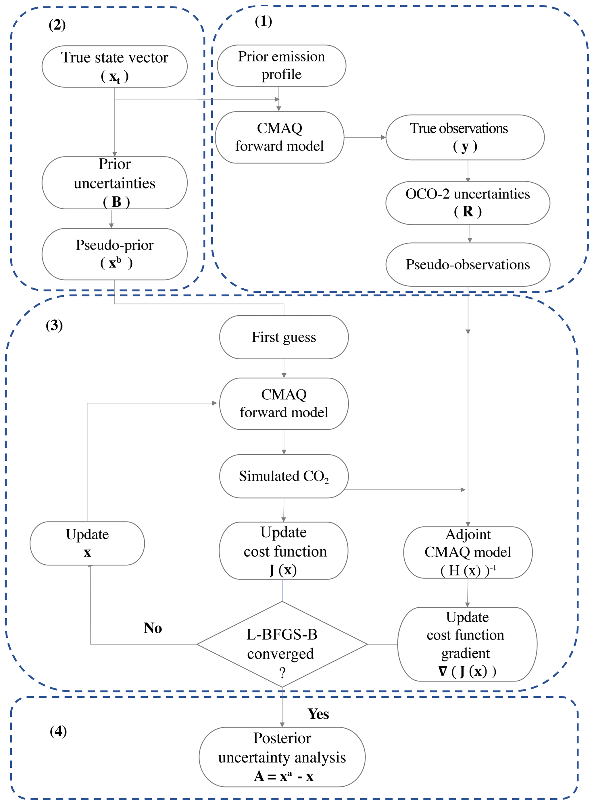
Figure 1Diagram representing an overview of the observing system simulation experiments (OSSEs) and how the inversion is performed using the L-BFGS-B minimization algorithm.
In this study the OSSEs were performed only for the months of March, June, September and December 2015. We ran an ensemble of five inversions for each month using different perturbations, generating five samples of the posterior probability density function (PDF). In the following subsections we describe the main ingredients of this procedure.
2.1 Inversion scheme
The inversion scheme for optimizing CO2 surface fluxes over Australia involves a Bayesian four-dimensional variational assimilation system. The system is a generalized minimization-based inverse-modelling framework, which can be applied to several potential models. We refer to it hereafter as “py4dvar”. py4dvar finds an optimal estimate of the CO2 surface fluxes (xa) that fits both observations (y) and the prior fluxes (xb) (Ciais et al., 2010; Rayner et al., 2019). Assuming Gaussian PDFs, finding this maximum a posteriori estimate is equivalent to minimizing the cost function J(x) shown in Eq. 1 (Rayner et al., 2019).
The first term in Eq. (1) represents the sum of squared differences between the control variable (x) and its prior or background state (xb). The second term measures the sum-of-squared difference between the model simulation, H(x), and observations (y) during the time window of the assimilation. The term H(x) is the function composition of an atmospheric transport operator and an observation operator. Both terms in Eq. (1) are weighted by their respective error covariance matrices (B and R), and the errors are assumed to be Gaussian and bias free. As mentioned in the previous paragraph, the minimum of J(x) is found by an iterative process rather than by an analytical expression. The minimization inside py4dvar is performed using the limited-memory BFGS (L-BFGS-B) algorithm, as implemented in the scipy python module (Byrd et al., 1995). The minimization algorithm, L-BFGS-B, requires values of the cost function and its gradient, which are calculated using the CMAQ forward model and the adjoint model, as shown in the third step in Fig. 1.
The gradient of the cost function in Eq. (2) is calculated using the adjoint of the CMAQ model (version 4.5.1; Hakami et al., 2007). We can observe that in the second term in Eq. (2), the adjoint model (HT) is applied to the vector , which is often called the “adjoint forcing”, or simply the “forcing”, and represents the error-weighted differences between the forward model and the observed concentrations. Applying the adjoint model to the forcing, running backward in time from ti−1 to t0, allows us to construct the gradient of the cost function, ∇xJ(x).
2.2 Choice of control variables
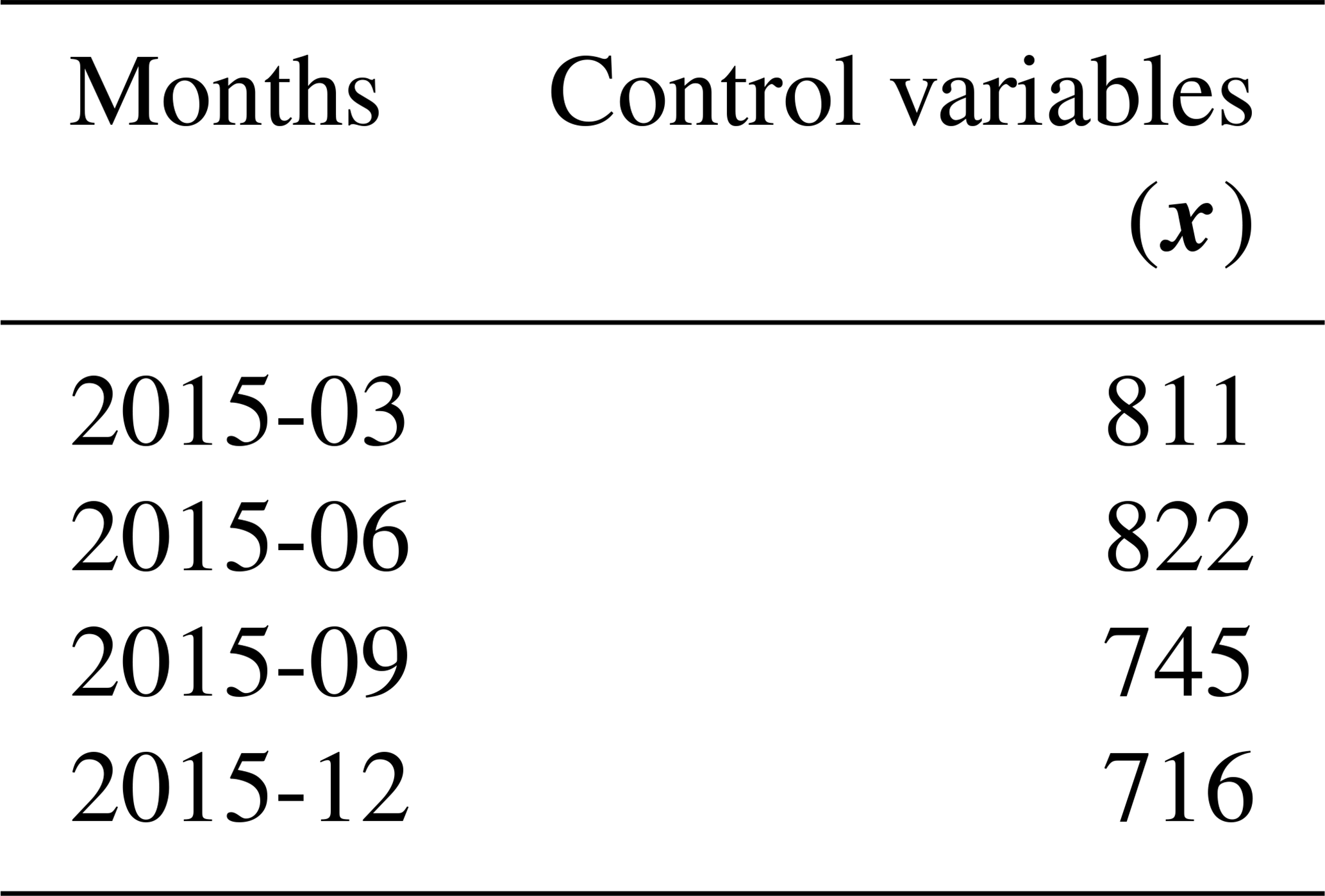
Our underlying physical variables are the monthly averaged fluxes at the spatial resolution of CMAQ (≈81 km). We do not split fluxes by day and night, consistent with only using daytime satellite observations, which are not subject to much influence by diurnal cycles in CO2 fluxes (e.g. Deng et al., 2014; Houweling et al., 2015). Like most previous studies (e.g. Chevallier et al., 2007; Baker et al., 2010; Basu et al., 2013; Crowell et al., 2019) we use spatially correlated prior uncertainties to account for systematic errors in flux estimates. The variables exposed to the minimizer are not the fluxes themselves but rather multipliers for the principal eigenvectors of B. We truncate the eigenspectrum at 99 % of the total variance; doing this significantly reduces the size of the control vector x (relative to if the control vector was comprised of the fluxes at each grid cell). This requires a different number of eigenvectors for different months (Table 1). The length of the control variables for our sensitivity experiments are defined in Table 6. Similar to Chevallier et al. (2005a), and because our inversion assimilation window is short, we also include (in the state vector for the inversion) a perturbation to the initial conditions (ICONs) of the CO2 concentration field. Because we are not interested in the analysis of this field, and in order not to significantly increase the size of the control vector, we added a scaling factor for the ICONs to our control variables , where i0 is the factor we solve for ICONs and en is the number of eigenvectors. The scaling factor was applied to the full three-dimensional concentration field. Some freedom in the initial condition avoids fluxes being unduly influenced by a mismatch in the initial concentrations. We assumed 1 % (≈4 ppm) uncertainties for the scaling factor.
Table 1Number of eigenvectors included in our control vector (x). Date format is YYYY-MM.
2.3 Observations and their uncertainties
We used OCO-2 level 2 satellite data (Lite File Version 9) distributed by the National Aeronautics and Space Administration (NASA) (available for download from https://oco2.gesdisc.eosdis.nasa.gov/data/s4pa/OCO2_DATA/, last access: 18 January 2020). We used the column-averaged dry air mole fraction of CO2, referred to as XCO2. We selected bias-corrected data, as described by Kiel et al. (2019). We used nadir and glint soundings over land that were flagged as good quality, except in some of our sensitivity experiments (described in Sect. 4) in which we excluded glint mode data. We computed a weighted average for all OCO-2 measurements using a two-step process similar to Crowell et al. (2019). The first step is to average all the soundings into 1 s intervals and the second is to average these 1 s averages into the CMAQ vertical columns (81 km × 81 km) for each satellite pass, where the transit time over the CMAQ grid cell is about 11 s. For the 1 s averaging process, the weighted averaging is defined in Eq. (3).
where is the squared reciprocal of the OCO-2 uncertainties (σi). To get the uncertainties of these averaged soundings, we considered three different forms of uncertainty calculation (similar to Crowell et al., 2019). First if we assumed that all errors are entirely correlated in a 1 s span, we can define the uncertainties as shown in Eq. (4).
However, and because the average shown in Eq. 4 is sometimes low, we also considered the standard deviation of the XCO2 measurements (here referred to as the spread, or σr, of the OCO-2 measurements). In other words, if the spread (σr) of the XCO2 measurements was higher than the XCO2 uncertainty (σi), we used the spread value as shown in Eq. (5). We did this because the spread in OCO-2 measurements may reflect real differences across the field within a 1 s time span.
Third, we also considered a baseline uncertainty (σb), based on an error floor (ϵ) over land and ocean, as shown in Eq. (6). We did this because sometimes we did not have enough OCO-2 soundings to compute a realistic spread. The values for our baseline uncertainties were taken to be 0.8 and 0.5 ppm over land and ocean, respectively. Finally, and after defining the uncertainties for the 1 s averages, we choose the maximum value between σs, σr and σb.
The second step was to take these 1 s averages and average them within the CMAQ vertical columns using Eq. 7.
where represents the squared reciprocal of the uncertainties average in the 1 s span (σj) and J is the number of those 1 s values. The average uncertainty over the CMAQ domain (Eq. 8) was similar to the procedure outlined for 1 s average in Eq. (4). However, we also added a term to represent the contribution of the model uncertainty (σm). We assumed that the model had a uncertainty of about 0.5 ppm. The observational error covariance matrix R was assumed to be diagonal.
After averaging the OCO-2 sounding over the CMAQ domain, we generated a set of pseudo-observations as described in step 1 of Fig. 1. In this process, we run the CMAQ model forward. We start with an assumed set of CMAQ inputs, which includes fossil fuel emissions, fires, land and ocean fluxes (see Sect. 2.4 for a description of these fluxes). Our py4dvar system takes in a vector x representing perturbations to the assumed emission profile, which is set to all be zeros in the “true case” and converts it into a format accessible to the CMAQ model (e.g. copying the monthly-average values into the hourly-resolution that the CMAQ model is configured to run with). These perturbations to the emissions (zero values in the true case) are then added to the assumed emission profile for CMAQ before the model is run to produce a four-dimensional CO2 concentration field, as is in step 2 of Fig. 1. Fourth, this modelled CO2 concentration field is then transformed using the OCO-2 observation space. Once it is transformed, we perturbed the “true observations” with Gaussian random noise to generate pseudo-observations as follows.
The first term of Eq. (9), ysim, represents the OCO-2- simulated observations using the true fluxes. The second term of Eq. (9), p, is a vector with the same size as ysim and contains normally distributed random numbers with mean zero and variance of one. Scaling p by the square root of R ensures that the resulting realization has the assumed error distribution.
2.4 Prior CO2 fluxes and their uncertainties
As is stated in Sect. 2.5, the CMAQ model needs hourly emissions to run forward in time. We use the atmospheric convention that a negative flux value indicates an uptake by the surface and a positive value means a release of carbon to the atmosphere. Our total fluxes were comprised of four datasets representing elements of the CO2 fluxes: terrestrial biospheric exchange, fossil fuels, fires and air–sea exchange. Hourly biosphere CO2 fluxes were calculated by combining two datasets: the net ecosystem exchange (NEE) at and daily resolution and the gross primary production (GPP) at and 3-hourly resolution from the Community Atmosphere Biosphere Land Exchange (CABLE) model (Vanessa Harverd, personal communication, 2018).
The post-processing of 3-hourly NEE data involved four steps. First, we calculated daily GPP. Then we used daily GPP to estimate the daily ecosystem respiration (ER); in terms of carbon balance, the ER can be calculated as . Finally, daily ER was assumed equal throughout the day and subtracted from 3-hourly GPP to obtain 3-hourly NEE. These 3-hourly NEE fluxes were interpolated to hourly resolution. Recall that for our OSSEs, only the uncertainties, not the values themselves, are used. Given that the optimization was performed to optimize monthly fluxes, the uncertainties were computed with monthly resolution. We assumed that the biosphere flux uncertainties were equal to the net primary production (NPP) simulated by CABLE, with a ceiling of 3 g C m−1 d−1 following Chevallier et al. (2010a).
Fossil-fuel CO2 emissions were obtained from the Fossil Fuel Data Assimilation System (FFDAS) (Rayner et al., 2010; Asefi-Najafabady et al., 2014). For this study, we used the 2015 FFDAS dataset (Kevin Robert Gurney, personal communication, 2018). The FFDAS uncertainty estimates were created by multiplying the FFDAS emissions dataset with a factor of 0.44. This factor was calculated by linear regression between the mean fluxes and the spread of an ensemble of 25 realizations of posterior CO2 fluxes, following Asefi-Najafabady et al. (2014). We did not directly use those realizations to get the posterior FFDAS uncertainties, because the realizations only contained emissions over land (i.e. excluding domestic, aviation, and maritime emissions). These “missing” emissions were taken from the Emissions Database for Global Atmospheric Research (EDGAR) (Olivier et al., 2005). The highest value of FFDAS uncertainty over land was 2.3 g C m−2 d−1 and over ocean was 0.5 g C m−2 d−1. This surprisingly large value over the ocean was a coastal point coinciding with Perth (Western Australia), where one of the largest and busiest general cargo ports in Australia is located.
Fire emissions were taken from the Global Fire Emission Database, version 4 (GFEDv4). This version of GFEDv4 provides gridded monthly fire emissions at 0.25∘ (van der Werf et al., 2017). The GFEDv4 product combines four satellite datasets: the Moderate Resolution Imaging Spectroradiometer (MODIS) burned area data product with active fires, data from the Tropical Rainfall Measuring Mission (TRMM) Visible and Infrared Scanner (VIRS) and the Along-Track Scanning Radiometer (ATSR). We used biomass-burning carbon emissions, a product based on GFEDv4 and the Carnegie Ames Stanford Approach (CASA) biosphere model (Randerson et al., 1996). Within the CASA model, fire carbon losses are calculated for each grid cell and month, based on fire carbon emissions based on burned area from the GFED dataset. We assumed uncertainties for GFEDv4 corresponding to 20 % of the biomass-burning carbon emissions.
Ocean CO2 fluxes were derived from the Copernicus Atmospheric Monitoring Service (CAMS) version 15r2 (Chevallier, 2016). The CAMS dataset is a global retrieval product, with a horizontal resolution of 3.75∘ in longitude and 1.875∘ in latitude at 3-hourly temporal resolution. Prior ocean fluxes estimated by CAMS were based on Takahashi et al. (2009). We assumed that the error statistics were uniform, 0.2 g C m−2 d−1, over ocean, as in Chevallier et al. (2010a).
After defining the emission profiles and their uncertainties, we incorporated spatial correlations into our prior error covariance matrix B. We assume no temporal correlations. This differs from Chevallier et al. (2010a), who used a temporal correlation length of 4 weeks; though, this would only introduce weak correlations among our monthly averaged fluxes. Following Basu et al. (2013, Sect. 3.1.1), the spatial correlation between grid points r1 and r2 was defined as
where d(r1,r2) is the distance (in km) between the two grid points, and L, the correlation length, was assumed to be 500 km over land and 1000 km over ocean following Basu et al. (2013).
After defining B, we performed an eigendecomposition, B=WTwW, where W is a matrix of eigenvectors and w is a diagonal matrix of corresponding eigenvalues. Figure 4a shows the cumulative percentage variance and demonstrates that 20 eigenvectors account for about 60 % of the variance in B. We truncate the eigenspectrum to retain 99 % of the overall variance. The number required varied each month but was at most 400, compared to approximately 6700 grid points. The main reason for this strong truncation is the large correlation length relative to the CMAQ grid resolution. We will test and discuss this later.
We solve the minimization with a change of variable xb. Given that our control vector x depends on the size of the multipliers of the principal eigenvectors of B, our vector xb was reconstructed (as is given in Eq. 11). This reconstruction includes a new vector q, which is normalized by the square root of the eigenvalues of B; this transformation involves minimization with respect to q, rather than xp.
This step (often called pre-conditioning) accelerates convergence. It also simplifies the system since, all target variables have unit standard deviation. In our case, where we solve for perturbations around a background state, they also have a true value of zero. Generating our prior flux for the inversion is achieved by defining a vector of normally distributed random numbers with unit standard deviation and zero mean. The process to generate the pseudo prior is represented in Eq. (11).
2.5 CMAQ model configuration
We used the CMAQ modelling system and its adjoint (version 4.5.1; Hakami et al., 2007) to conduct numerical simulation of the atmospheric CO2 concentration over the Australian region. The CMAQ modelling system is an Eulerian (gridded) mesoscale chemical transport model (CTM), initially created for air quality studies. It has been previously used to characterize the variability of CO2 at fine spatial and temporal scales (Liu et al., 2014). The choice of an older version of the CMAQ modelling system (cf. the latest version, v5.3) relates to the requirement of the model adjoint (needed to calculate the gradient of the cost function in the inversion).
We treat CO2 as an inert tracer, neglecting its chemical production (Folberth et al., 2005; Suntharalingam et al., 2005). Thus modelled concentrations are determined only by emissions, the atmospheric transport (horizontal and vertical advection and diffusion), and initial and boundary conditions. Initial and boundary conditions were interpolated from atmospheric CO2 concentration data from the Copernicus Atmospheric Monitoring Service (CAMS) global CO2 atmospheric flux inversions (Chevallier et al., 2010a). These data have a resolution of 3.75∘ in longitude and 1.875∘ in latitude with 39 vertical layers in the atmosphere; this dataset was also the basis for the oceanic fluxes used in the prior. The CMAQ chemical transport model (or CCTM) also requires 24-hourly three-dimensional emission data (recall that in our py4dvar system we solve for a perturbation around these background CO2 fluxes). Here our background CO2 fluxes were generated by adding the four CO2 flux fields described in Sect. 2.4: carbon exchange between biosphere and atmosphere, carbon exchange between ocean and atmosphere, fossil-fuel emissions, and biomass-burning emissions.
(Morrison et al., 2009)(Iacono et al., 2008)(Iacono et al., 2008)(Monin and Obukhov, 1954)(Tewari et al., 2007)(Janjić, 1994)(Grell and Dévényi, 2002)Table 2Physics parameterizations used in the Weather Research and Forecasting (WRF) model setup.

The CMAQ model is an offline model, and thus requires three-dimensional meteorological fields as inputs for the transport calculations. We simulated meteorological data using the Weather Research and Forecasting model (WRF) Advance Research Dynamical Core WRF-ARW (henceforth, WRF) version 3.7.1 (Skamarock et al., 2008). Details on the physics schemes used in our WRF configuration are shown in Table 2. Our domain has a horizontal resolution of 81 km and 32 vertical layers from the surface up to 50 hPa. The numerical simulation was carried out on a single domain (i.e. non-nested) of 89×99 grid cells.
The meteorological initial conditions were based on the ERA-Interim global atmospheric reanalysis (Dee et al., 2011), which has a resolution of approximately 80 km on 60 vertical levels from the surface up to 0.1 hPa. Sea surface temperatures were obtained from the National Centers for Environmental Prediction/Marine Modeling and Analysis Branch (NCEP/MMAB). The WRF model was run with a spin-up period of 12 h. The initial spin-up period stabilizes the model, that is, the inconsistencies between the initial and boundary conditions diminish in this period.
The WRF modelled meteorology was nudged towards the global analysis fields above the boundary layer. The default grid-nudging configuration was used; that is, nudging coefficients were assumed to be 10−4 s−1 for wind and temperature and 10−5 s−1 for moisture, as suggested by Deng and Stauffer (2006). Nudging has been widely used in mesoscale modelling as an effective and efficient method to reduce model errors (Stauffer and Seaman, 1990). It relaxes the model simulations of wind, temperature and moisture towards driving conditions, preventing model drift over a long-term integration.
The WRF model output was post-processed by the Meteorology-Chemistry Interface Processor (MCIP) version 4.2 (Otte and Pleim, 2010). MCIP prepares the meteorological fields in a form required by CMAQ and performs horizontal and vertical coordinate transformation. In this process, we removed the outermost six rows and columns from each edge of the WRF model domain, so the horizontal CMAQ domain was set up (with 77×87 grid cells). This was done to prevent numerical instabilities in the “relaxation zone” (the exterior rows and columns of the horizontal domain), where the lateral meteorological boundary conditions and the WRF model's internal physical processes both contribute.
2.6 Observation operator: CMAQ CO2 simulations and OCO-2 measurements
As is seen in Eq. (1), we need to compare the CMAQ simulated CO2 concentration with OCO-2 satellite retrievals. As outlined in Sect. 2.3, we averaged observations to approximate the observed XCO2 for any CMAQ grid cell observed by OCO-2. To compare modelled and observed concentrations, we used the Eq. (12) (Rodgers and Connor, 2003; Connor et al., 2008) to convolve the simulated CO2 concentration with the relevant averaging kernels, as follows:
where xa is the OCO-2 a priori, h is a vector of pressure weights, hj is the mass of dry air in layer j divided by the mass of dry air in the total column, is the averaging kernel of OCO-2, xa,j is the OCO-2 a priori profile, and xm is the simulated profile from the CMAQ model. In our py4dvar system, the first and second terms in Eq. (12) represent an “offset term”. The OCO-2 averaging kernel is defined on 20 pressure levels and we interpolate these to the CMAQ vertical levels.
In this section, we present an assessment of the uncertainty reduction resulting from the flux-inversion process. First, we present an analysis of the convergence of our minimization and evaluate the information content (degrees of freedom for signal) of our OSSE simulation experiments. This is followed by an analysis of the uncertainty reduction categorized by MODIS land coverage. Finally, we present seven sensitivity experiments to determine the robustness and consistency of our inversions.
3.1 Convergence diagnostic
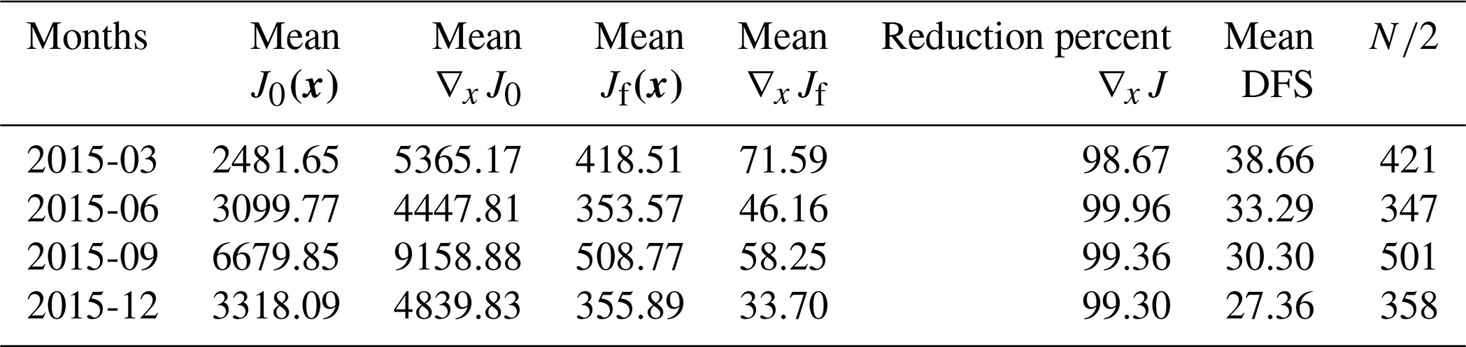
One interesting diagnostic of the convergence is to compare the cost function at the end of the optimization to its expected theoretical value. In a consistent system, the theoretical value of the cost function at its minimum should be close to half the number of assimilated observations, assuming all error statistics are correctly specified (Tarantola, 1987, p. 211). Table 3 shows the mean (across our five realizations) of the cost function J(x) and its gradient norm ∇xJ. For example, with 842 observations, the theoretical value should be 421. We see that the theoretical value is reached to within a few percent for all months. We see a corresponding decrease in the gradient norm by about 99 %.
Table 3Convergence diagnostics of the inversion system using an ensemble of five independent OSSEs for March, June, September and December 2015. Date format is YYYY-MM.
3.2 Degrees of freedom for signal
The number of degrees of freedom for signal (DFS) in our OSSEs is another useful diagnostic of the inversion (Rodgers, 2000, Eq. 2.46). The DFS quantifies the number of independent pieces of information that the OCO-2 measurements can provide given the prior information. In our experimental framework, we computed the DFS following Chevallier et al. (2007, Sect. 3.4.):
where xa represents our posterior estimates. Table 3 shows that on average the DFS in the prior for our four months is about 30. This value is consistent with Fig. 4a and b, which shows that only about 20 eigenvalues account for 60 % of the variance in our prior error covariance matrix. The inversion cannot add much information to other components, limiting the DFS. Australia is a special case in this respect since most of the continent comprises semi-arid and arid regions. We assumed that land flux uncertainties are driven by NPP, as simulated by CABLE. Thus, the prior uncertainty will be small in arid and semi-arid regions.
3.3 Spatial distribution of uncertainty reduction
The uncertainty reduction between the posterior and prior fluxes is a useful way to evaluate the potential of satellite data to constrain CO2 fluxes. We calculated the percentage uncertainty reduction following (Chevallier et al., 2007, Sect. 3.5.), as follows:
where σa and σb are the posterior and prior standard deviations, respectively. Figure 5 displays the monthly uncertainty reduction in CO2 fluxes for (a) March, (b) June, (c) September and (d) December 2015. We have masked areas with mol m−2 s−2. We also mask areas with negative uncertainty reduction. Such uncertainty increase is simply a result of the small number of realizations. We will now describe the magnitude and spatial patterns in the uncertainty reduction, and in Sect. 3.4 we will discuss the uncertainty reduction aggregated by land cover class.
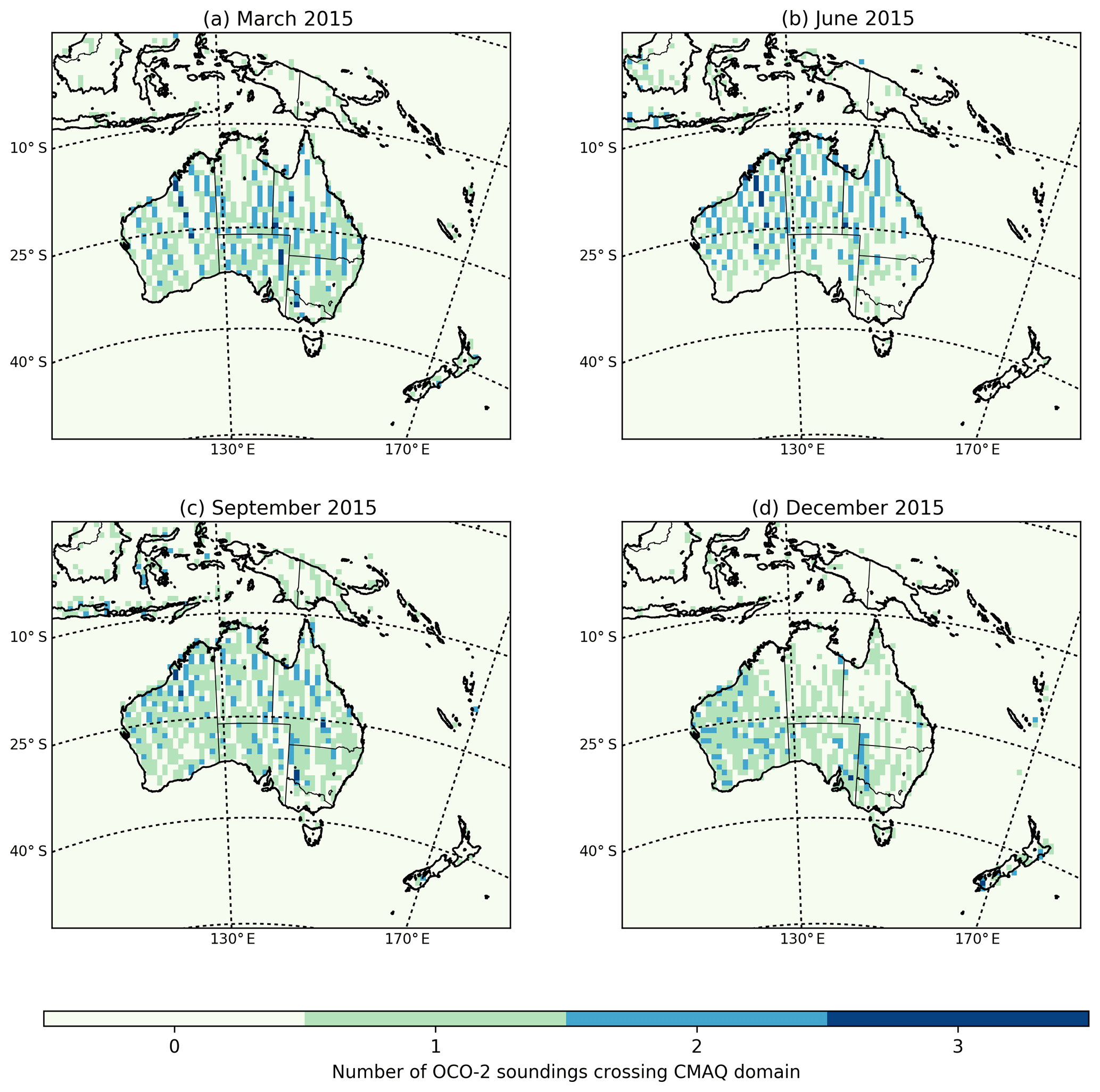
Figure 2Spatial distribution of OCO-2 soundings (land nadir and glint data) over the CMAQ domain for March, June, September and December 2015.
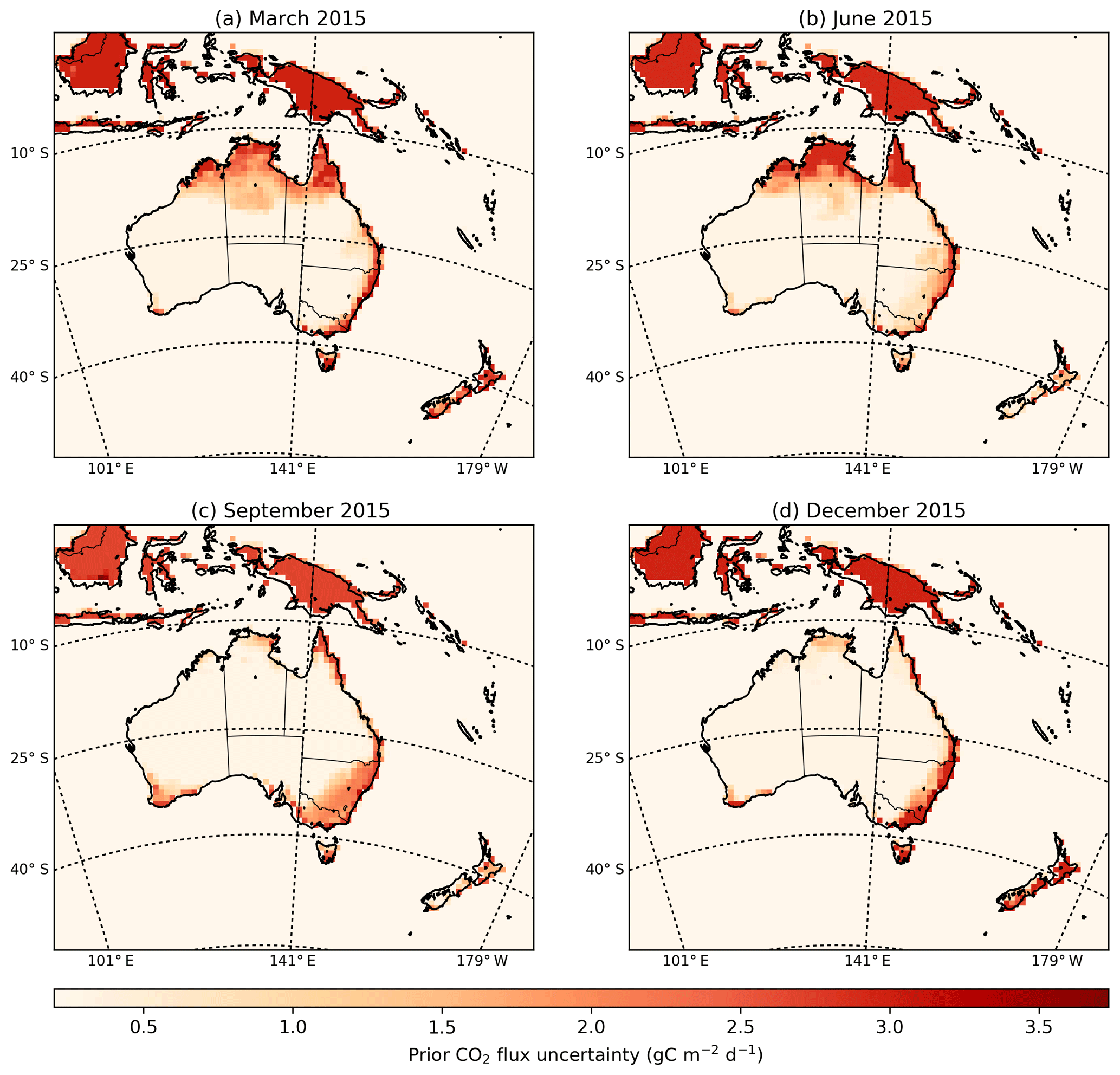
Figure 3Monthly mean of CO2 prior uncertainties accounting for the major terms in the CO2 budget (anthropogenic fluxes, fires, land and ocean exchange) (in units of g C m−2 d−1).
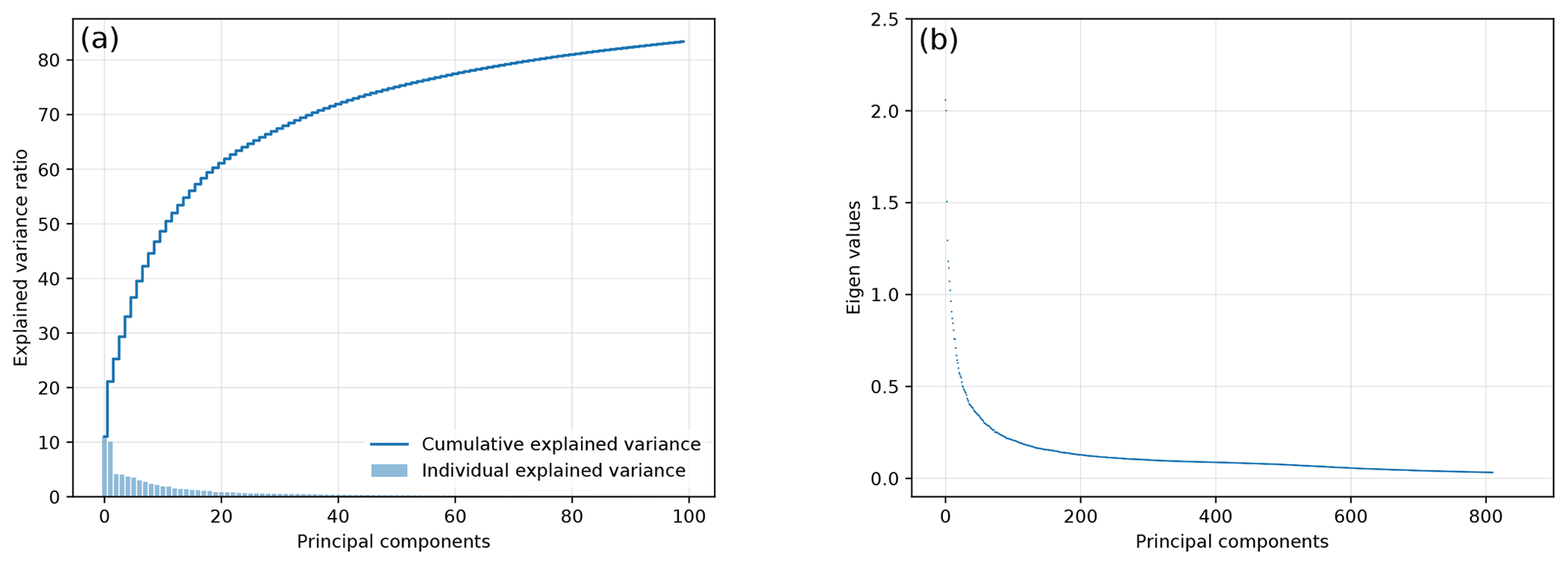
Figure 4The cumulative percentage variance explained (a) and the eigenvalues (b) in the prior error covariance matrix.
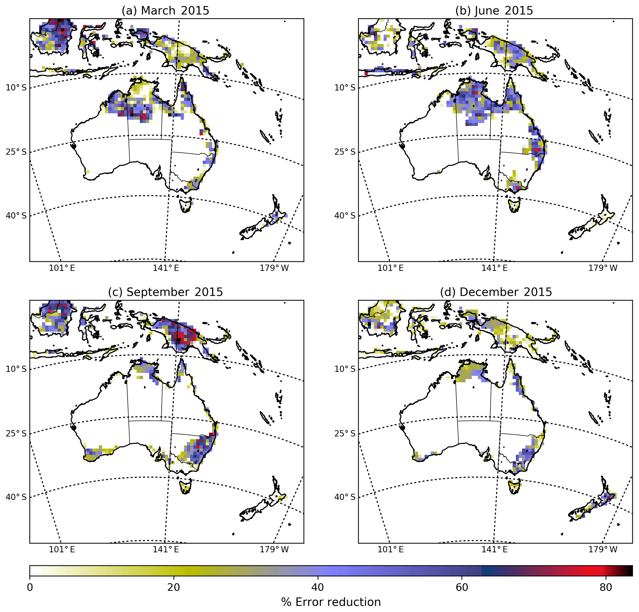
Figure 5The percentage error reduction of the monthly-mean CO2 surface fluxes for March, June, September and December 2015 over the CMAQ model domain. The percentage of error reduction is defined as , with σa and σb representing, respectively, the posterior and prior uncertainties of the CO2 fluxes emissions.
In March, the largest uncertainty reductions (Fig. 5a) are located in the north of Australia. In this area, the uncertainty reduction is greater than 30 %, reaching values up to 80 %. We note that the regions with the largest reduction in uncertainty coincide with the locations with high prior uncertainty (Fig. 3). In June 2015 (Fig. 5b), for instance, the largest uncertainty reduction was found in the north, north-east, east and south-east of Australia, where values range between 70 % and 80 %. Uncertainty reductions in September (Fig. 5c) are higher compared to June in the south-east of the country, ranging between 70 % and 80 %. This is consistent with the fact that September is in the middle of the growing season in this part of Australia and our prior uncertainties are driven by NPP. Also, more satellite soundings are available for this region in September compared to other months. The uncertainty reduction in December (Fig. 5d) decreases in the north of Australia to a range of 20 %–30 %. This is likely due to the fact that relatively few OCO-2 soundings are available in that month (Fig. 2), due to increased cloud coverage during the wet season in northern Australia. This is discussed further in the next section.
3.4 Uncertainty reduction over Australia by MODIS land cover classification
To get a better understanding of the constraint on CO2 surface fluxes provided by OCO-2, we aggregated the prior and posterior fluxes into six categories over Australia: grasses and cereal (GC), shrubs (SH), evergreen needleleaf forest (ENF), savannah (SAV), evergreen broadleaf forest (EBF), and unvegetated land (UN). We used the MODIS Land Cover Type Product (MCD12C1) Version 6 data product. The distribution is shown in Fig. 6. After aggregating fluxes for each realization we calculated standard deviations and uncertainty reductions following Eq. (14).
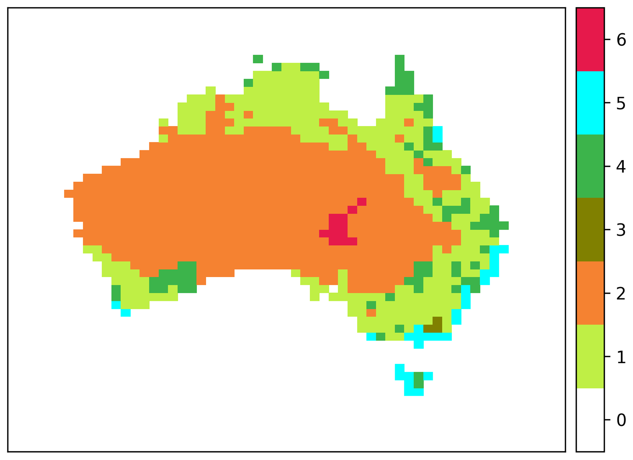
Figure 6Aggregation of land cover classes over CMAQ domain using MODIS Land Cover Type Product (MCD12C1) Version 6 data product. Colour bars represent each category: (0) ocean, (1) grasses and cereal, (2) shrubs, (3) evergreen needleleaf forest, (4) savannah, (5) evergreen broadleaf forest, and (6) unvegetated land.
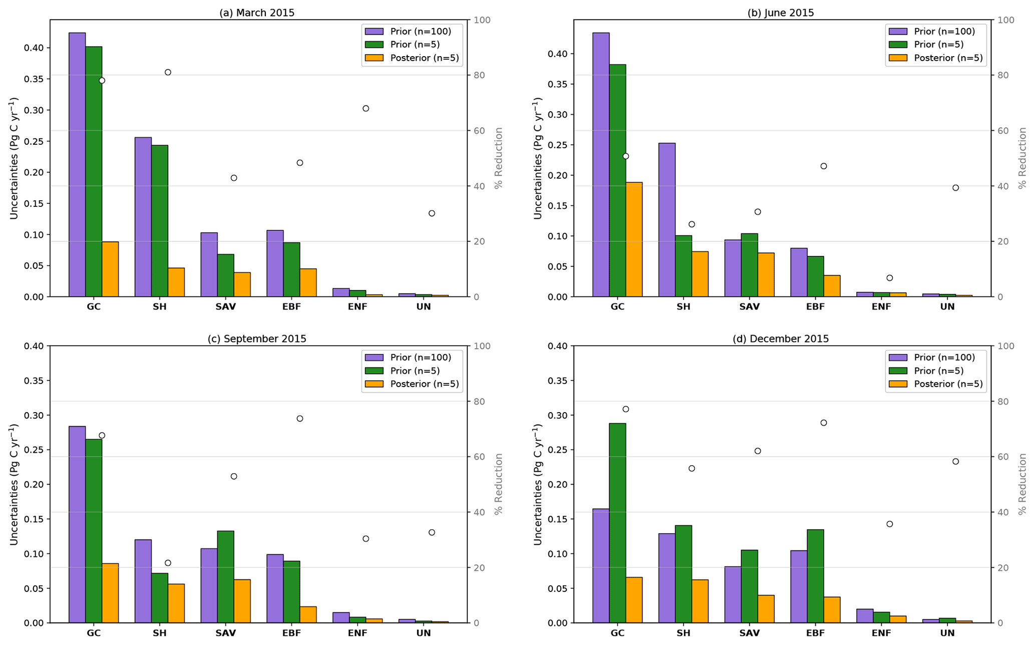
Figure 7Prior and posterior uncertainties (in Pg C yr−1) aggregated over five different classes over the Australian domain using MODIS Land Cover Type Product (MCD12C1). Green and orange bars represent the prior and posterior uncertainties of five realizations, respectively, while the purple bar represents prior uncertainties of 100 realizations. Circles show the percentage of uncertainty reduction by each category.
The bar chart in Fig. 7 shows the prior (green bar) and the posterior (orange bar) uncertainties of our five realizations (in Pg C yr−1) split into six land-use classes for (a) March, (b) June, (c) September and (d) December 2015. The uncertainty reduction for each land-use class and each month is represented by circles. Also shown is a second estimate of the prior uncertainties, comprising 100 realizations (purple bar). The prior of 100 realizations is plotted to assess the representativity of the five random prior realizations of the prior uncertainties. We see clearly in each figure that with only five realizations we can represent quite well our assumed prior uncertainties (we should also note that, due to computational limitation, the uncertainty reduction is based only on these five realizations).
The largest uncertainty reduction in March is over SH (81 %). The large uncertainty reduction is likely due to the large number of OCO-2 soundings in this region (464 observations). The next largest uncertainty reductions are over GC (78 %) and ENF forest (68 %) likely due to the relatively large NPP in these regions (Fig. 3a).
June shows less uncertainty reduction for GC (51 %) compared to March, likely due to the smaller number (one third as many) of OCO-2 soundings (Fig. 2) in southern Australia. similarly, uncertainty reduction over the SH ecotype decreases. Due to the small number of realizations, however, this percentage of reduction might not be representative of this region. For this category, we can see that the prior uncertainty with five realizations is about 0.1 Pg C yr−1, whereas with 100 realizations it is about 0.25 Pg C yr−1. Uncertainty reduction over SAV is about 31 %, similar to the percentage of reduction found in March. Even though we found relatively few soundings over EBF and ENF in June, uncertainty reductions for these regions are 47 % and 7 %, respectively. The reduction over UN areas is about 39 %, again demonstrating the potential of OCO-2 data to constrain fluxes.
In September the most significant uncertainty reduction was found over EBF (74 %) and GC (68 %) compared with all other months, associated with the peak of the growing season in much of Australia. Uncertainty reductions in these categories are much larger due to the increase of OCO-2 soundings in south-eastern Australia (see Fig. 2c). The uncertainty reduction over areas designated as SAV and ENF is about 53 % and 30 %, respectively. Over areas classified as SH and UN, we see a weaker uncertainty reduction of 22 % and 33 %, respectively.
Similar to September, in December we found the largest uncertainty reductions over EBF (72 %) in line with the structure of the uncertainties seen in south-eastern of Australia in (Fig. 3c). The percentage of uncertainty reduction found over GC (77 %) may not represent the precise percentage for this category (given the small number of realizations used). For this category, we see that the prior uncertainties of 100 realizations is about 0.17 Pg C yr−1, whereas with five realizations it is about 0.28 Pg C yr−1. We would expect to have a smaller uncertainty reduction for this category due to scarcity of soundings available in the north and north-eastern Australia for this month, likely due to cloudiness associated with the wet season. Uncertainty reductions found over areas classified as SH, SAV and ENF were 56 %, 62 % and 36 %, respectively. Different to other months, the uncertainty reduction over UN is about 58 %.
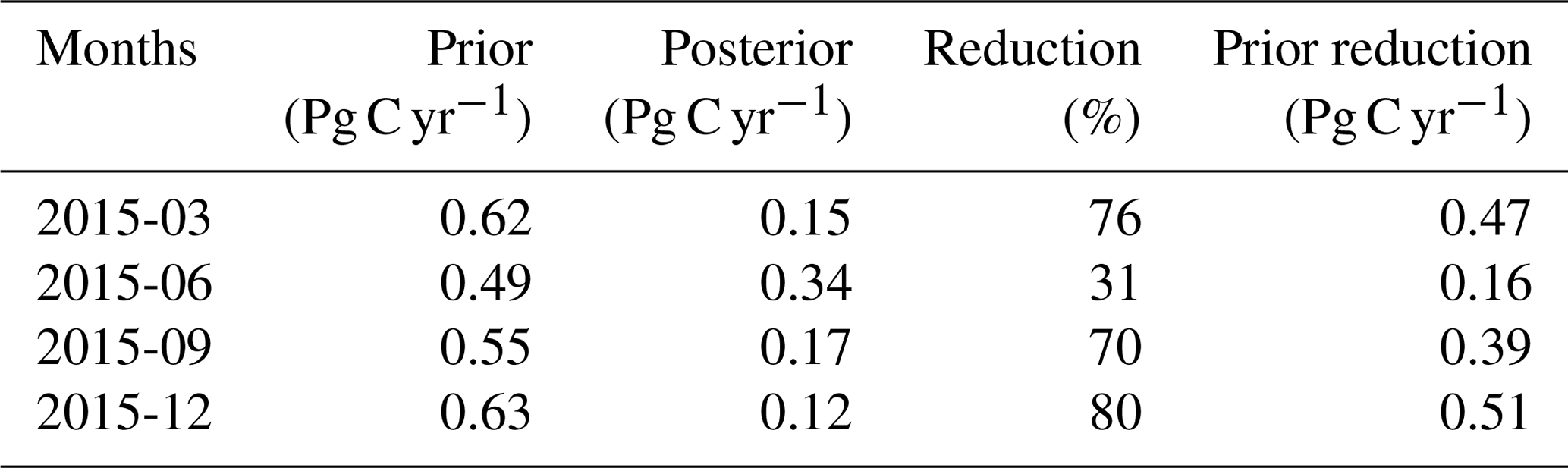
3.5 Uncertainty reduction in the total Australian CO2 flux
Table 4 shows the standard deviation of the total CO2 flux uncertainty over Australia for the four months in which inversions were run. Months with the largest uncertainty reductions are found in December (80 %), March (76 %) and September (70 %). In contrast with these results, the smallest reduction is found in June (31 %). The last of these results is not surprising, since June is the month with the smallest number of OCO-2 soundings (for this month we only find 694 observations compared to September and March, with 1002 and 842 soundings, respectively).
Table 4Prior and posterior uncertainties (in Pg C yr−1) for an ensemble of five realizations aggregated over the Australian continent. Date format is YYYY-MM.
Differences in the uncertainty reduction between months not only depend on the number of soundings and the structure of the uncertainty but also other variables (e.g. wind direction). Coastal grid points present a problem for our inversion when the wind direction comes from the ocean because our system only assimilates data over land). Prevailing winds in this coastal zone restrict the ability of OCO-2 to constrain surface fluxes (Figs. S1–S3 in the Supplement).
To assess the robustness and consistency of the previous results, we performed seven different sensitivity experiments (S1, S2, S3, S4, S5, S6-A, S6-B), which are summarized in Table 5. These experiments follow the same randomization approach shown in Sect. 2 but with the following changes.
-
S1 tests the effect of reducing the correlation lengths in our prior error covariance matrix B. The correlation length was changed from 500 to 50 km over land, and from 1000 to 100 km over the ocean. By reducing the correlation length, the number of retained eigenvectors increased from 811 (control experiment) to 4101. The shorter correlation lengths allow for a larger selection of possible flux structures, requiring more eigenvalues to capture the possible variance.
-
S2 assesses what percentage of uncertainty reduction of the Australian flux is affected by excluding glint land observations from our inversion. Our control cases treat land nadir and glint data as one single dataset because of the small offset between them. The number of observations influences the footprint coverage and therefore the number of fluxes we can solve. In this particular experiment, we would expect a smaller uncertainty reduction of Australian flux, because the number of observations has been reduced from 842 to 419.
-
S3 evaluates the effect of having uniform uncertainties over land and a simplified structure of B. In this case, we assumed uncertainties of 3 g C d−1 over land with correlation lengths of 5 km over land and 10 km over ocean. This change effectively transforms B into a diagonal matrix.
-
S4 tests the impact of adding a bias of 3.3 ppm to the OCO-2 observations. Here, biases were calculated by taking the differences between the raw and bias-corrected XCO2 values found in the OCO-2 retrieval product. We performed this experiment because some studies (e.g. Chevallier et al., 2007) indicate that just a few tenths of a part per million bias in the observations are enough to prevent the inversions from converging on optimal fluxes.
-
S5 tests the impact of introducing a mean absolute bias of 0.21 Pg C yr−1 to prior fluxes. In this experiment, the prior bias were created using a normal Gaussian random perturbation of the prior uncertainty. For all five realization, biases were introduced as constant component.
-
S6-A tests the impact of adding bias in the boundary conditions (BCs). We increased the BCs simulated by adding a uniform offset of 0.5 ppm on each grid cell. In this case, we did not solve for BCs in the inversion.
-
S6-B assesses the impact of incorporating BCs in the inversion system to deal with the bias introduced in S6-A. BCs were introduced to the control vector as eight boundary regions (representing the upper and lower areas of the north, south, east and west sides of the rectangular domain). We did not solve the BCs in the same way that we solve for the surface fluxes, as they are not among the key results (i.e. BCs were treated as nuisance variable). In this case, we gave the optimizer the ability to modify the BCs while it is optimizing surface fluxes. For this test, we assumed a uniform uncertainty of 1 ppm s−1. This is applied as an additive perturbation to temporally and spatially varying concentration boundary conditions based on the CAMS global CO2 simulations.
Table 5A brief description of the sensitivity OSSEs performed for March 2015.
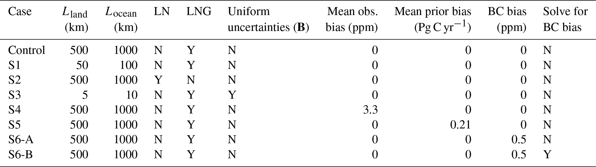
Land nadir data is defined as LN, and land nadir and glint data as LNG.
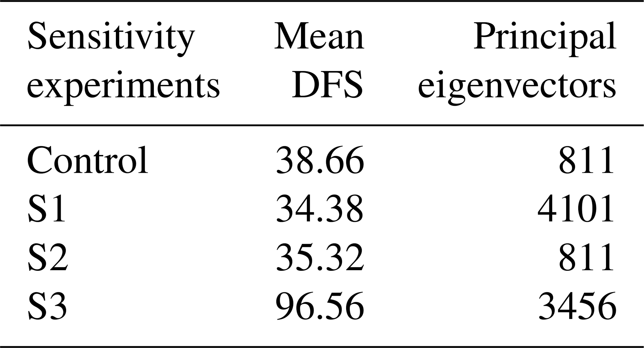
4.1 Degrees of freedom for signal
Table 6 shows the number of retained eigenvalues from B and the DFS for sensitivity experiments S1, S2, S3 and control cases. Experiment S1 shows that merely reducing correlation lengths does not lead to extra information being resolved by the observations. S2 shows that, as expected, subtracting observations from our inversion resolves less information on fluxes. Experiment S3 (in which we reduce correlation lengths but also increase the uncertainty on many grid points) demonstrates an increase in the number of components resolved by the observations. The comparison of S1 and S3 suggests it is the low uncertainty rather than the smoothness imposed by the uncertainty correlations that limits the DFS.
Table 6Number of degrees of freedom for signal (DFS) in the prior flux uncertainty and the number the principal eigenvector in the prior error covariance matrix for sensitivity experiments S1, S2 and S3.
4.2 Spatial distribution of uncertainty reduction over Australia
Figure 8 shows the spatial distribution of the uncertainty reduction at grid-scale over Australia for sensitivity experiments S1, S2 and S3. These figures should be compared to Fig. 5a (control case). Experiment S1 shown in Fig. 8a demonstrates that the correlation length plays a significant role in the uncertainty reduction. A lower correlation length yields a lower reduction of the uncertainties. For example, the error reduction over the productive areas in northern and north-eastern Australia is between 0 % and 20 % compared to the control experiment's 40 %–80 %. This implies that longer correlation length scales allow for information to be effectively “transferred” in space, thus pooling data over a wider region and magnifying the benefit from the assimilation.

Figure 8Maps of the percentage of error reduction for the three sensitivity cases. (a) Using only nadir OCO-2 sounding and correlation lengths 50 and 100 km. (b) Using “nadir” and “glint” OCO-2 sounding and correlation lengths of 500 and 1000 km. (c) Uniform uncertainties over land and ocean, and correlation lengths of 5 and 10 km.
Experiment S2 (Fig. 8b) illustrates that decreasing the number of observations also reduces the percentage of reduction per grid cell. The uncertainty reduction (40 %–60 %) is much weaker than the control experiment. These results complement Table 6, where the DFS decrease from 38.66 (control experiment) to 35.32 (S2).
Experiment S3 (Fig. 8c) shows how the structure and magnitude of the prior uncertainty influence uncertainty reduction. The uncertainty reductions are distributed almost uniformly across Australia, and their values range between 0 % and 20 %. Our assumption of a linear relationship between uncertainty and NPP means much of Australia has negligible impact on the prior uncertainty in the control case. This result shows the importance of that assumption. Assuming equal uncertainty across Australia may have a significant impact on the final total flux estimate, because most of the continent is largely composed of arid and semi-arid land. The small percentage of uncertainty reduction is due to the negligible correlation length assumed in the prior error covariance matrix.
4.3 Uncertainty reduction over Australia by MODIS land cover classification
Figure 9 shows the uncertainty reduction for the sensitivity cases S1, S2, and S3 aggregated by ecotype. There is good consistency between the geographical distribution (Fig. 8) and these spatial aggregates. Thus for case S1, the uncertainty reductions were found to be small compared to the results in the control experiment (Fig. 7a). For example, the sensitivity case S1 in Fig. 9a shows uncertainty reductions over GC and UN are about 30 % and 1 %, respectively. No uncertainty reductions are observed over SH, SAV, EBF and ENF. Because of an insufficient number of realizations, for these particular categories, we found a negative error reduction. In these land-use classes, we display the posterior to be equal to the prior uncertainty.
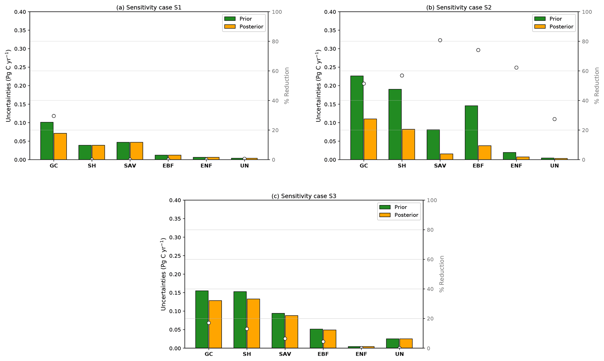
Figure 9Sensitivity experiments for the prior and posterior uncertainties (in Pg C yr−1) aggregated over six different classes over the Australia domain using MODIS Land Cover Type Product (MCD12C1).
Similarly, case S2 (Fig. 9b) displays significantly weaker uncertainty reductions for some of the six land-use classifications compared to the control experiments (Fig. 7a). For instance, the fractional uncertainty reductions over GC and SH reach values of about 51 % and 57 %, respectively. In the control experiment in (Fig. 7a) these values were 78 % and 81 %, respectively. As mentioned in the previous section, the stronger posterior reduction is due to the correlation length in the prior covariance and an increase of the OCO-2 soundings over Australia. Findings in the sensitivity case S3 (Fig. 9c) show similar results to those found in sensitivity case S1: the smaller the correlation length, the less efficient the inversion.
4.4 Uncertainty reduction in the total Australia CO2 flux uncertainty
Uncertainty reduction of the total Australian CO2 flux for sensitivity experiments S1, S2 and S3 are shown in Table 7. Experiment S1 shows that the regional flux uncertainty in Australia was only reduced by ∼9 % compared to the control case (which was 76 %). In this test, we can see again the importance of the choices of the correlation length in B. We saw in Table 6 that by decreasing the spatial correlation to 5 km over land, we increase the number of principal components. Given the small number of realizations and an increase in the number of components in the prior, we expect that this estimate of the uncertainty reduction may be less representative using our randomization approach.
Table 7Prior and posterior uncertainties (in Pg C yr−1) for an ensemble of five realizations.
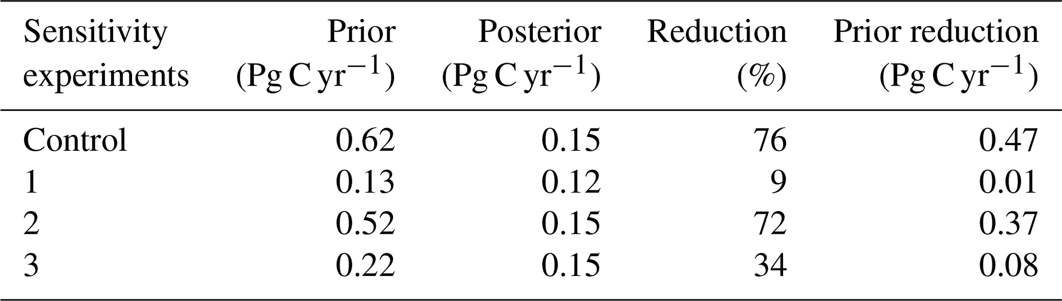
Experiment S2 shows an uncertainty reduction over Australia from 73 % compared to 76 % (control case). This small shift in the percentage of reduction is related to the number of soundings found in the northern region of Australia. By removing glint land data from our observations, we are reducing the coverage of surface flux footprints.
Experiment S3 demonstrates the same artefact as S1, though the generally higher prior uncertainties in S3 result in a higher uncertainty reduction for the total Australian flux. In this case, the assimilation reduces the total uncertainty to 34 %.
4.5 Impact of OCO-2 biases on the posterior fluxes
We mentioned in Sect. 4 that potential biases in the observations prevent the inversions from converging on optimal fluxes. The results of experiment S4 confirms that biases in the observations do indeed affect the resulting posterior fluxes. After adding biases of about 3.3 ppm, our inversion produced a posterior flux, which was bias by approximately 5.0 Pg C yr−1 over Australia. This value indicates that in order to obtain an accuracy of 0.1 Pg C yr−1 in the total Australian flux, bias in the observation must be reduce roughly to 0.07 ppm. This sensitivity case shows us the importance of minimizing biases in the observations if the goal is to estimate accurately CO2 fluxes. Figure 10 illustrates the impact of the observational biases on the posterior mean fluxes in each of the six MODIS land-use categories. Significant biases are observed over SH (1.7 Pg C yr−1), GC (1.4 Pg C yr−1), and EBF (0.9 Pg C yr−1). For each category, the inversion system only generates positive flux biases, consistent with the direction of the bias in the observations. Our results are mainly due to large biases we prescribed in the observations. Finally, we found that uncertainty of prior and posterior were 0.68 and 0.25 Pg C yr−1, respectively. Given the magnitudes of the prior uncertainties (and hence biases in this case), this result is consistent with the control case.

Figure 10Posterior bias of monthly CO2 flux induced by OCO-2 bias categorized by MODIS ecotype.
4.6 Unbiased prior CO2 flux
Results of experiment S5 are illustrated in Fig. 11. This figure shows the monthly-mean biases (black diamonds) added to our prior true fluxes (assumed to be 0.0 Pg C yr−1) categorized by MODIS ecotype. In this figure, we can see that after performing the inversion we can recover successfully the mean of our true fluxes (dashed grey line). On average the total biases added to our Australian prior flux was about 0.21 Pg C yr−1 (using a conversion factor of 2.12 Pg C ppm−1, this value is equivalent to adding 0.1 ppm bias). After performing the inversion, the posterior mean bias was reduced to 0.024 Pg C. The distribution of the fluxes across the different land-use classes (centred around zero; Fig. 11) reflects the fact that biases added to our prior were randomly distributed. We added negative biases to GC and SH (−0.12, −0.05 Pg C yr−1) and positive bias to SAV and EBF (−0.05, 0.05 Pg C yr−1). We can see clearly in this figure that the inversion system is able to handle negative and positive biases.
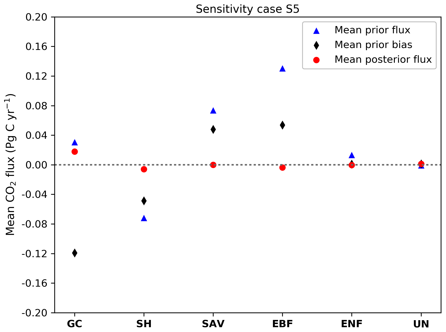
Figure 11Prior (blue) and posterior (red) monthly-mean CO2 flux of a ensemble of five realizations and monthly-mean prior bias (black) added to the true prior fluxes (dashed grey line). Note: results are shown for adding the same biases to our five realizations.
4.7 Impact of boundary condition biases on the posterior fluxes
Unlike global flux inversions, regional flux inversions are sensitive to lateral boundary conditions (BCs). To explore how sensitive our system is to biased BCs, we ran two further sensitivity experiments (collectively termed “S6”). In sensitivity experiment S6-A we increased the BCs by adding 0.5 ppm to each boundary grid cell. Findings of this experiment show that our system is indeed sensitive to the altered BCs. Adding an extra 0.5 ppm to the BCs yields a posterior bias in Australia of about −0.7 Pg C yr−1. These findings are in line with the values found in sensitivity case S4, but in a opposite direction. The negative value of the bias means the inversion system is trying to reduce the fluxes to compensate for the positive bias in the BCs. The mean posterior bias flux for each land category is shown in Fig. 12.
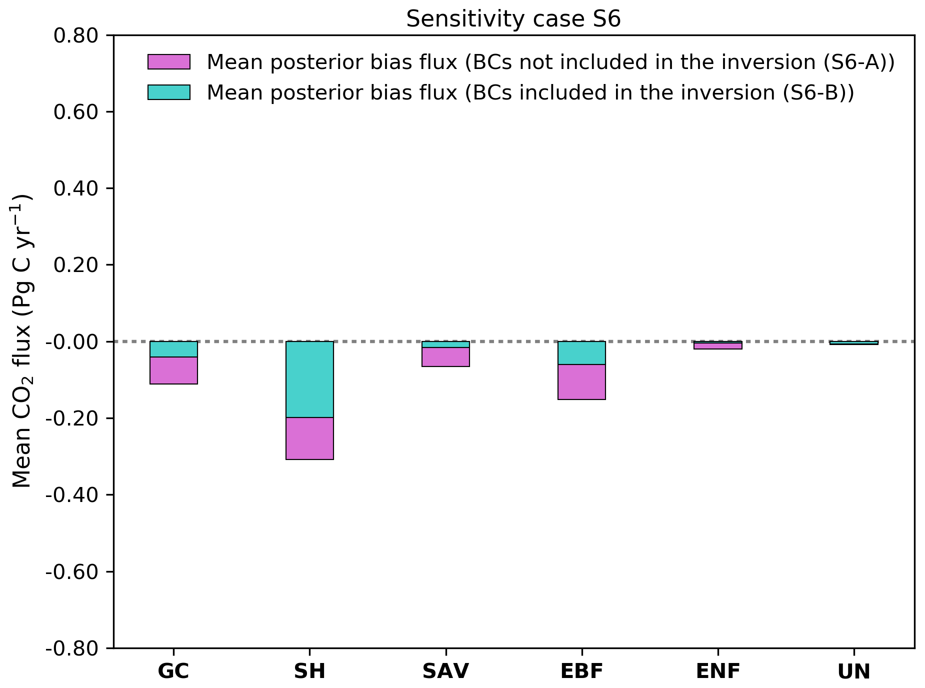
Figure 12Posterior bias of monthly CO2 concentration induced by changes in the lateral boundary conditions categorized by MODIS ecotype.
4.8 Solving for the boundary condition in the inversion
Experiment S6-B was designed to see if the inversion could correct for biases in the boundary conditions given additional parameters to optimize. After solving for BCs in the inversion, the biases introduced to BCs in S6-A were corrected. We analysed the corrections by looking at the bias of the posterior flux for each land-use category. Figure 12 shows that the decrease of biases over GC was significant. In this category biases were reduced from −0.11 to −0.019 Pg C yr−1. Similar results were found over SAV, EBF and ENF, where biases were also reduced. Biases over SH does not show much improvement. In this category biases decreased only from −0.30 to −0.20 Pg C yr−1. After a wind-rose analysis for 10 selected locations around the coast in west Australia (Figs. S1–S3), we found that the small reduction of the biases in this category is explained by the orientation of the wind in March. When winds come from ocean, the inversion loses the ability to correct the wrong BCs. The treatment of the bias in BCs is relatively simple, with a goal of introducing relatively few additional parameters into the control vector. The experimental design assumes that these biases are constant in time and across large areas of the domain. The biases in the BCs were generated with the same framework as was used to solve them (i.e. fully specified by eight parameters). In reality, error in BCs will vary in both space and time. Thus, the results here are indicative but suggest that biases (as opposed to fluctuations) at least can be accounted for in such a system.
One key uncertainty in any OSSE is the realism of the observational uncertainties. One simple test involves performing a limited inversion of data and assessing whether the cost function (Eq. 1) is consistent with the number of observations. Unlike the OSSE, this is not guaranteed; in the “real-data” inversion, there are likely errors in the atmospheric transport and the initial and boundary conditions. To test this, we performed an inversion for March 2015 using nadir and glint data. As mentioned in Sect. 2.2, we added a scaling factor for the initial condition to our target variables to test the inversion.
Figure 13 shows a histogram of residuals between the CMAQ model simulations using optimized fluxes and OCO-2 observations. We can see that the monthly-mean bias was reduced from 0.49 to −0.01 ppm, with a decrease in the root-mean-square error (RMSE) from 1.08 to 0.89 ppm. While these are based on the same data that were assimilated and do not necessarily show that the posterior fluxes are closer to the truth, it does show that our system is self-consistent. The cost function J(xa) at its minimum is 418.52, close to half the number of observations (842).
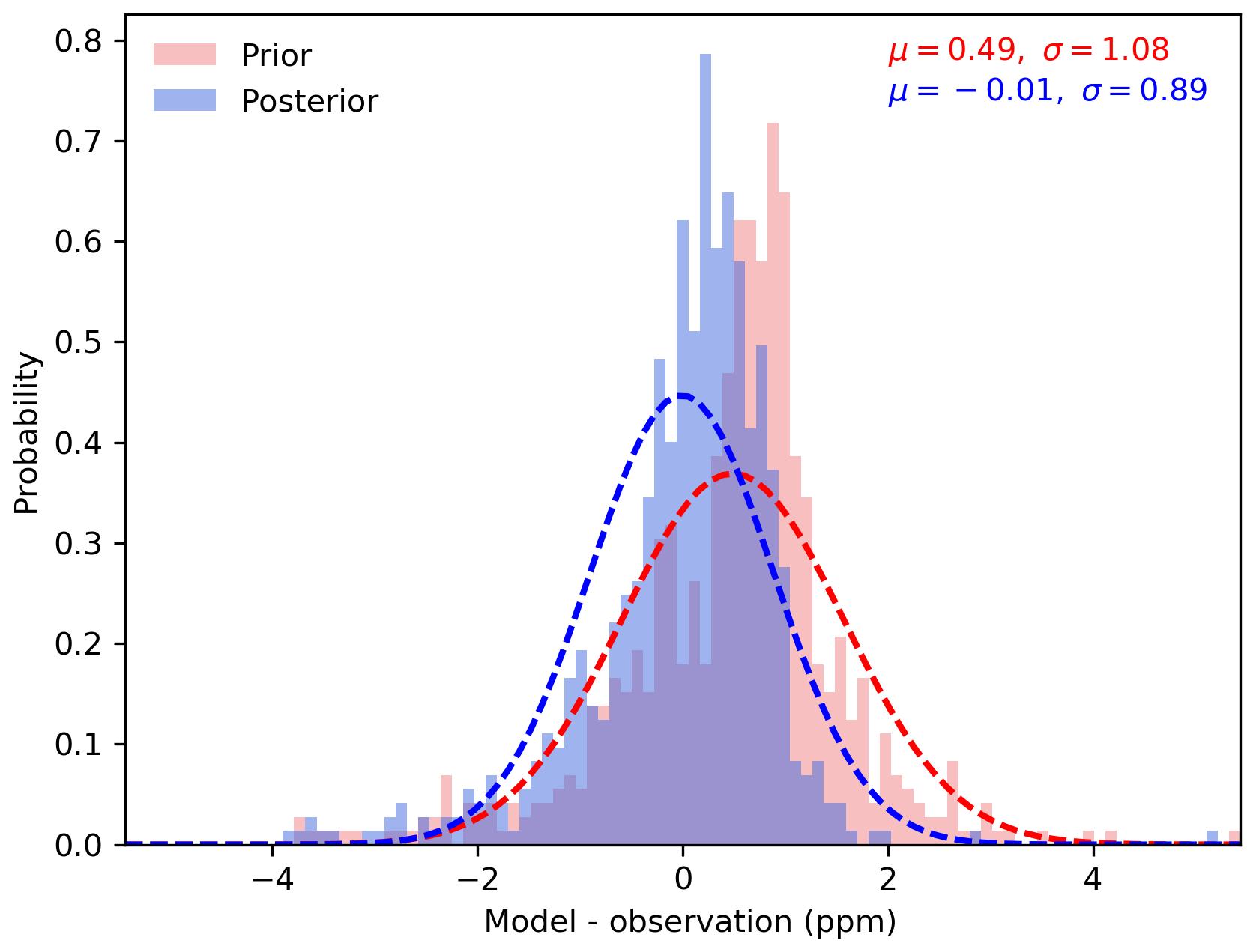
Figure 13The distribution of the difference between simulated and observed XCO2 (in ppm). The red histogram presents the prior XCO2 simulated minus the observed XCO2, whereas the blue histogram presents the posterior XCO2 simulated minus the observed XCO2. Mean differences and standard deviations are indicated in the legend.
In this paper, we quantified the potential uncertainty reduction in monthly CO2 fluxes when assimilating OCO-2 satellite retrievals with a regional-scale model at approximately 80 km grid resolution. If we compare our results shown in Fig. 5 against, for example, Fig, 2 of Chevallier et al. (2007) we see that our grid-scale uncertainty reductions are higher than those by Chevallier et al. (2007) by almost a factor of 2, using nadir and glint data over land. In Chevallier et al. (2007), uncertainty reductions in Australia are about 30 %–50 % over productive areas, while in this study they reach 60 %–80 %. One possible explanation for this is the lower observational uncertainty assumed in our study, averaging 0.6 ppm compared with 2 ppm assumed by Chevallier et al. (2007) before OCO-2 was launched. We can also compare our results with those for the in situ network studied by Ziehn et al. (2014). At the national scale, Ziehn et al. (2014) suggested an uncertainty reduction of 30 %, while we see 76 % for our control case.
Our results must be interpreted with caution, because, like all OSSEs, they depend strongly on assumed inputs (such as B and R), which are difficult to characterize. In particular, we have assumed that the CABLE NPP (Haverd et al., 2013a) is a good proxy for biospheric net flux uncertainty, following Chevallier et al. (2010a). Chevallier et al. (2010a) used a different model and a different domain, so these assumptions may require further testing in our model configuration and region of interest. In future, we could compare CABLE simulations against eddy-covariance CO2 flux measurements following Chevallier et al. (2012). Characterization of the prior biospheric flux over semi-arid regions in Australia is critical to account for the inter-annual variability of these ecosystems (Poulter et al., 2014). Recent studies (e.g. Poulter et al., 2014) have suggested that the semi-arid regions in Australia could become an important driver of the carbon cycle in comparison with ecosystems dominated by tropical rainforests.
Sensitivity experiments S1 and S3 show that the uncertainty reduction in CO2 surface fluxes over Australia is sensitive to a combination of both magnitude and spatial distribution of the uncertainty, as well as the choice of the correlation length scale. We saw in case S1, for example, that by reducing the correlation length in B, we do not necessarily increase the number of degrees of freedom (DFS) in our prior compared to the control. These findings suggest that the number of DFS in our prior fluxes depends more on the spatial distribution of error variance than on the assumed correlation length-scale. These results are much clearer in experiments S3, where the distribution of the uncertainty is uniform across Australia. In this case, we see that the number of DFS increases by increasing the magnitude of the uncertainty across Australia. In sensitivity case S2, we saw that by subtracting glint data, our system was able to solve for fewer DFS in the fluxes compared to the control experiment.
Sensitivity experiment S4 shows that the existence of biases in the observations has a significant impact on our posterior flux estimate. Adding biases to our simulated OCO-2 observation prevents our inversion from converging on optimal fluxes. We saw in Sect. 4.5 that when adding biases (corresponding to an average increase of 3.3 ppm) to the observation, the posterior flux is also biased by about 5.0 Pg C yr−1. Our results are in agreement with Chevallier et al. (2007, 2010a) and show that regional biases in column-averaged CO2 can significantly bias our posterior fluxes. Similar results are found in experiment S6-A, which looked at biases in boundary conditions. Adding 0.5 ppm to the boundary conditions also has an impact on our posterior fluxes. Increased BCs resulted in negative bias in the posterior fluxes and to a degree that was consistent with sensitivity case S4. These findings suggests that our regional flux inversion is sensitive to boundary conditions; therefore, in a real inversion, controls on boundary conditions should be included in the state vector in addition to the surface fluxes.
Results in sensitivity case S5 shows that biased prior fluxes satisfy the theoretical assumption in the variational optimization similar to using an unbiased prior case. We demonstrated that our system is able to handle the impact of possible biases in the CMAQ model that might contaminate the resulting posterior fluxes.
Another direction for future work would be to explore the impact of a finer temporal and horizontal resolution on the resulting fluxes. Model simulations at higher spatio-temporal resolutions have been shown to have better agreement with observations, partly on account of allowing for a better representation of the measurements. (Law et al., 2004; Peylin et al., 2005; Patra et al., 2008). However, as we saw in Sect. 2.3, we found it necessary to average OCO-2 soundings before assimilating in the system. To simplify this process, the averaging process removed any 1 s soundings that spanned multiple grid cells in the CMAQ domain. This is about 7 km in along-track distance. If we use a finer resolution than 80 km, we could remove more soundings and thus weaken our constraint.
We emphasize again that our study quantifies the uncertainty but not the realism of our posterior flux estimates. The assessment of posterior fluxes from assimilation of real data will be the subject of an upcoming paper. This requires comparison with independent concentration data or, if available, flux estimates at comparable scales.
We have performed an observing system simulation experiment for the retrieval of CO2 fluxes over Australia using OCO-2 data and a regional-scale flux-inversion system. The main findings indicate that OCO-2 nadir and glint (version 9) data can provide a moderate (≈30 %) to significant (>70 %) constraint on the Australian CO2 flux uncertainty in 2015 (for most months studied). We saw that these reductions at a grid-point resolution reached values of about 90 %, with the largest uncertainty reductions being observed over biologically productive areas. Small uncertainty reductions are found over arid and semi-arid ecosystem, where we assumed the prior uncertainties were small. These reductions only become significant when aggregating by land-use classifications (e.g. shrubs 20 %–80 % ). For future work, it is relevant to consider a better characterization of our prior uncertainties in this region to account for the inter-annual variability of the carbon cycle in these semi-arid regions. Sensitivity experiments show that uncertainty reductions are quite sensitive to the assumed prior correlations but less sensitive to the spatial distribution of prior uncertainties. Moreover, we also saw that by excluding glint data from the assimilated observations, we reduce the coverage of the surface flux footprint and therefore the uncertainty reduction of the total Australian flux. It seems likely, therefore, that this combination of land and glint data can help quantify the Australian carbon cycle, provided simulations are sufficiently realistic. Finally, we showed that such OSSEs are useful to test the potential of the inversion to possible biases in the observation, prior and boundary conditions. Our future work will focus on the application of this assimilation system to estimate CO2 surface fluxes in Australia as a contribution to the REgional Carbon Cycle Assessment and Processes (RECCAP) project.
Table A1Convergence diagnostic of the inversion system using an ensemble of five independent OSSEs for March 2015 (∇xJ0 and ∇xJ0 represent the initial cost function and its gradient at the beginning of the optimization and ∇xJf and ∇xJf are for the end of the optimization).

Table A2Convergence diagnostic of the inversion system using an ensemble of five independent OSSEs for June 2015 (∇xJ0 and ∇xJ0 represent the initial cost function and its gradient at the beginning of the optimization and ∇xJf and ∇xJf are for the end of the optimization).
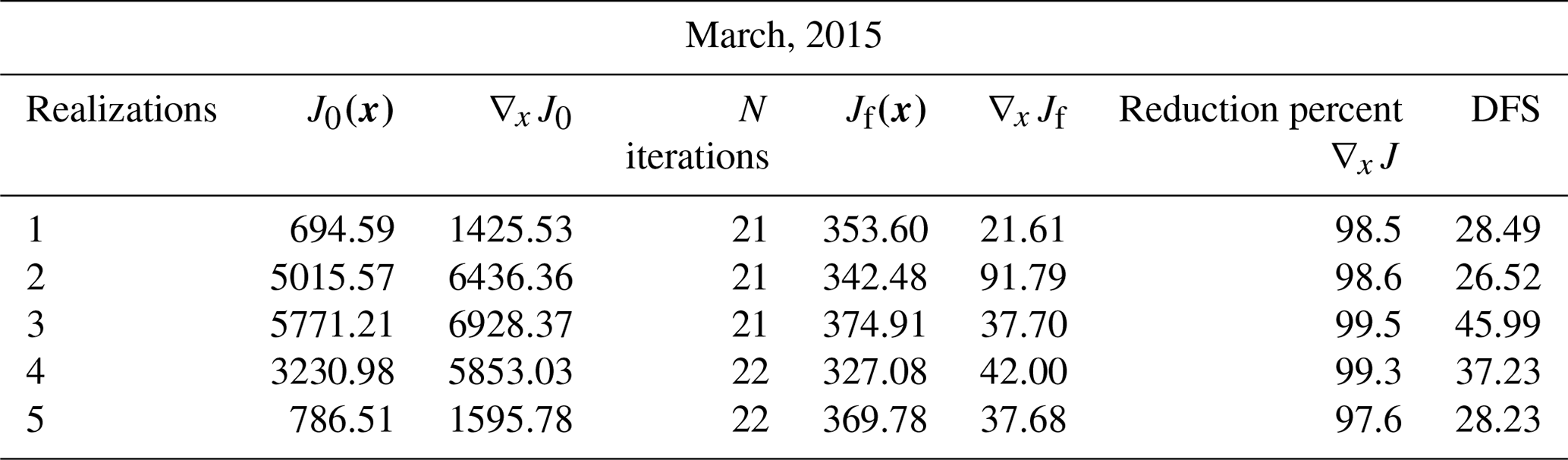
Table A3Convergence diagnostic of the inversion system using an ensemble of five independent OSSEs for September 2015 (∇xJ0 and ∇xJ0 represent the initial cost function and its gradient at the beginning of the optimization and ∇xJf and ∇xJf are for the end).
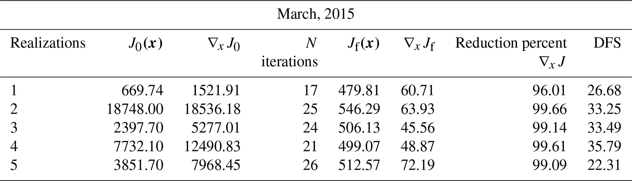
Table A4Convergence diagnostic of the inversion system using an ensemble of five independent OSSEs for December 2015 (∇xJ0 and ∇xJ0 represent the initial cost function and its gradient at the beginning of the optimization and ∇xJf and ∇xJf are for the end of the optimization).
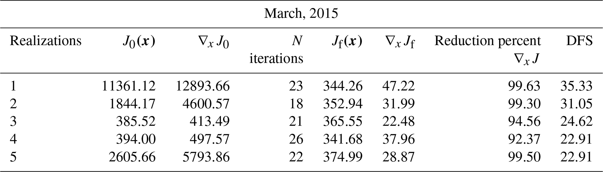
Table B1Uncertainty reduction of total CO2 Australian flux (in Pg C yr−1) classified by MODIS ecotype (March, 2015).
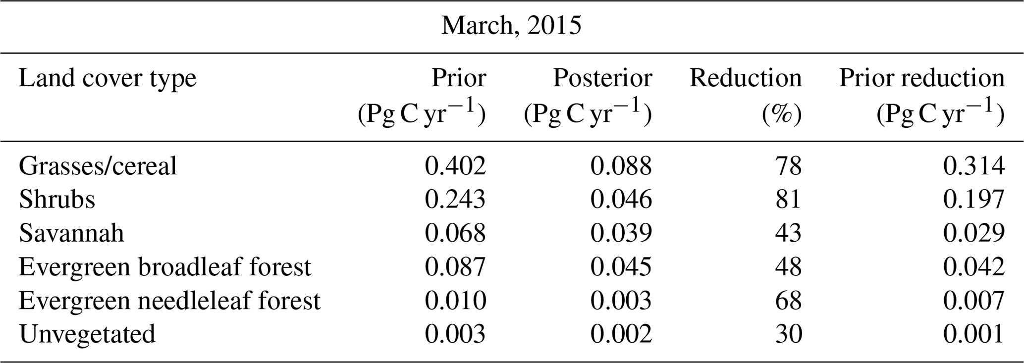
Table B2Uncertainty reduction of total CO2 Australian flux (in Pg C yr−1) classified by MODIS ecotype (June, 2015).
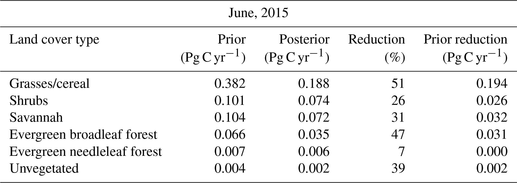
Table B3Uncertainty reduction of total CO2 Australian flux (in Pg C yr−1) classified by MODIS ecotype (September, 2015).

Table B4Uncertainty reduction of total CO2 Australian flux (in Pg C yr−1) classified by MODIS ecotype (December, 2015).
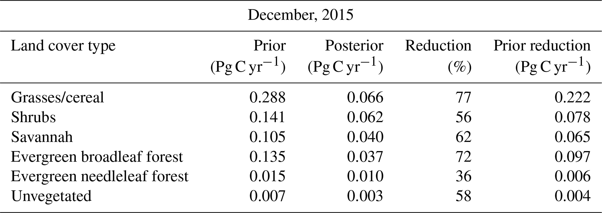
Table C1Convergence diagnostic of sensitivity case (1) after the inversion using an ensemble of five independent OSSEs for March 2015 (∇xJ0 and ∇xJ0 represent the initial cost function and its gradient at the beginning of the optimization, and ∇xJf and ∇xJf represent them at the end of the optimization).
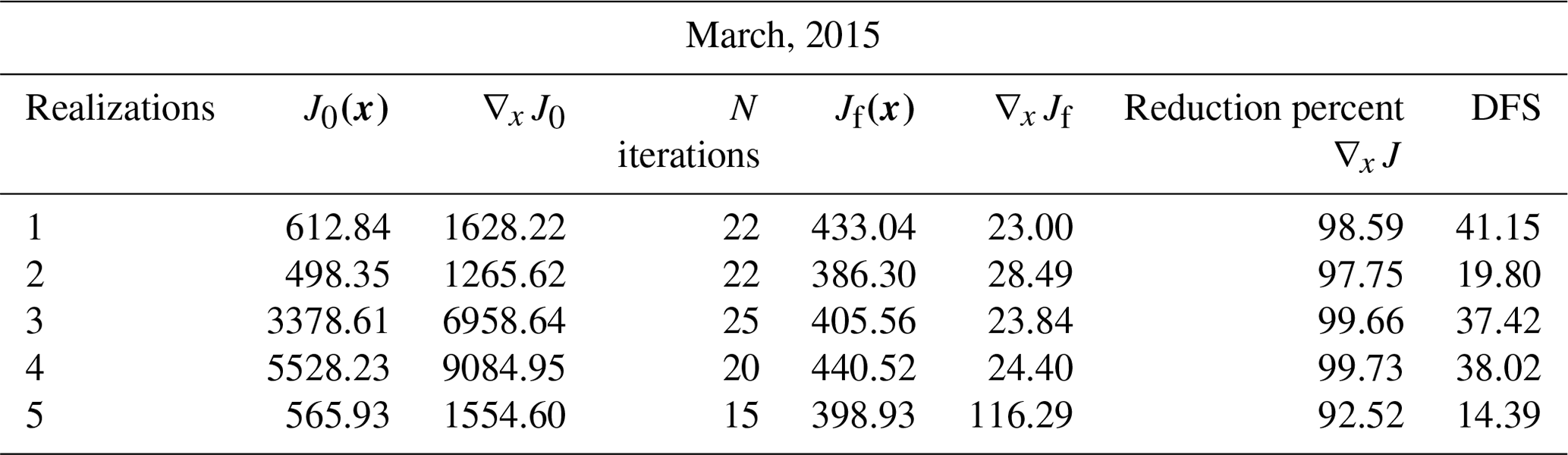
Table C2Convergence diagnostic of sensitivity case (2) after the inversion using an ensemble of five independent OSSEs for March 2015 (∇xJ0 and ∇xJ0 represent the initial cost function and its gradient at the beginning of the optimization, and ∇xJf and ∇xJf represent them at the end of the optimization).
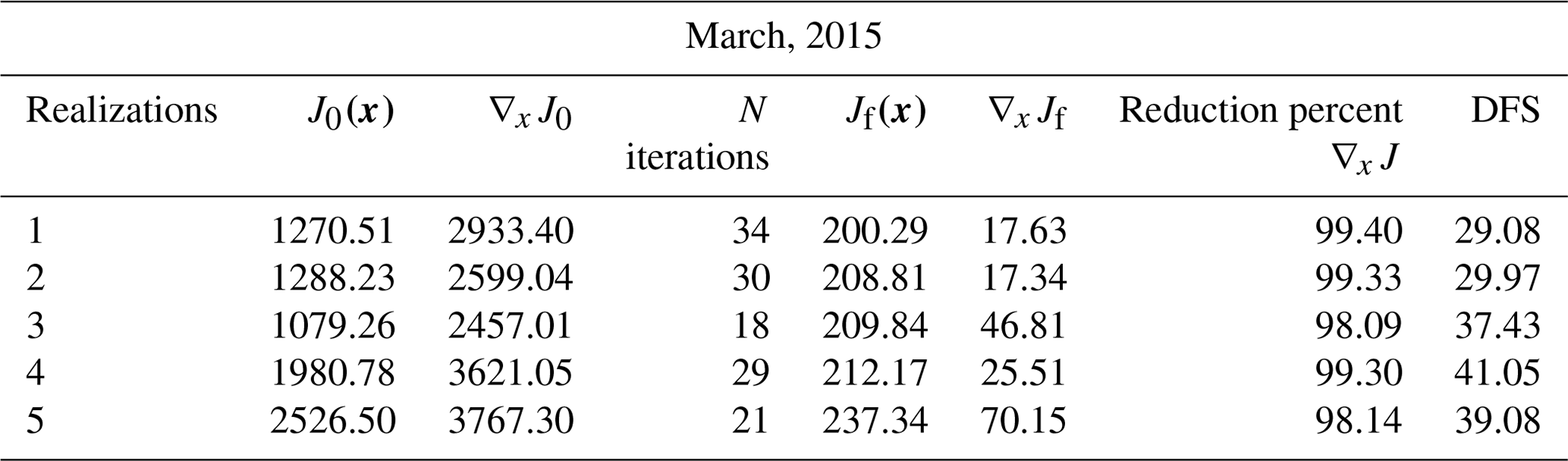
Table C3Convergence diagnostic of sensitivity case (3) after the inversion using an ensemble of five independent OSSEs for March 2015 (∇xJ0 and ∇xJ0 represent the initial cost function and its gradient at the beginning of the optimization, and ∇xJf and ∇xJf represent them at the end of the optimization).

Table D1Sensitivity case (1): uncertainty reduction of total CO2 Australian flux (in Pg C yr−1) classified by MODIS ecotype (March, 2015).
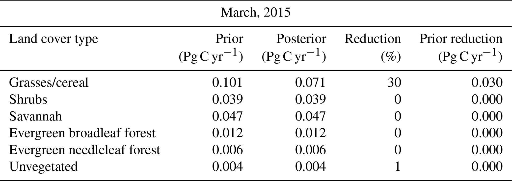
Table D2Sensitivity case (2): uncertainty reduction of total CO2 Australian flux (in Pg C yr−1) classified by MODIS ecotype (March, 2015).

Table D3Sensitivity case (3): uncertainty reduction of total CO2 Australian flux (in Pg C yr−1) classified by MODIS ecotype (March, 2015).

The inversion system for this work was performed in py4dvar code, which was written by Steven Thomas, available at https://github.com/steven-thomas/py4dvar (Thomas, 2020).
The supplement related to this article is available online at: https://doi.org/10.5194/acp-20-8473-2020-supplement.
YV performed all the OSSEs, including pre- and post-processing of data, and was responsible for developing the paper. ST was the principal developer of the py4dvar code with overall scientific guidance with additional analysis code from PR and JS. PR and JS also contributed to the writing of the article.
The authors declare that they have no conflict of interest.
This project was undertaken with the assistance of resources and services from the National Computational Infrastructure (NCI), which is supported by the Australian Government, and the resources of the High-performance Computing Centre of the University of Melbourne, SPARTAN (Lafayette et al., 2016). We acknowledge the contribution of the CMAQ adjoint team in providing us with the model code. We acknowledge the effort of Vanessa Haverd from CSIRO in providing us with the Australian biosphere carbon flux data.
This research has been supported by the National Commission for Scientific and Technological Research (CONICYT) scholarship, Becas Chile (grant no. 72170210), the Education Infrastructure Fund of the Australian Government, and the Australian Research Council (ARC) of the Centre of Excellence for Climate Extreme (CLEX, grant no. CE170100023).
This paper was edited by Yugo Kanaya and reviewed by three anonymous referees.
Arora, V. K., Boer, G. J., Friedlingstein, P., Eby, M., Jones, C. D., Christian, J. R., Bonan, G., Bopp, L., Brovkin, V., Cadule, P., Hajima, T., Ilyina, T., Lindsay, K., Tjiputra, J. F., and Wu, T.: Carbon-concentration and carbon-climate feedbacks in CMIP5 earth system models, J. Climate, 26, 5289–5314, https://doi.org/10.1175/JCLI-D-12-00494.1, 2013. a
Asefi-Najafabady, S., Rayner, P. J., Gurney, K. R., McRobert, A., Song, Y., Coltin, K., Huang, J., Elvidge, C., and Baugh, K.: A multiyear, global gridded fossil fuel CO2 emission data product: Evaluation and analysis of results, J. Geophys. Res.-Atmos., 119, 10213–10231, https://doi.org/10.1002/2013JD021296, 2014. a, b
Baker, D. F., Bösch, H., Doney, S. C., O'Brien, D., and Schimel, D. S.: Carbon source/sink information provided by column CO2 measurements from the Orbiting Carbon Observatory, Atmos. Chem. Phys., 10, 4145–4165, https://doi.org/10.5194/acp-10-4145-2010, 2010. a, b
Basu, S., Guerlet, S., Butz, A., Houweling, S., Hasekamp, O., Aben, I., Krummel, P., Steele, P., Langenfelds, R., Torn, M., Biraud, S., Stephens, B., Andrews, A., and Worthy, D.: Global CO2 fluxes estimated from GOSAT retrievals of total column CO2, Atmos. Chem. Phys., 13, 8695–8717, https://doi.org/10.5194/acp-13-8695-2013, 2013. a, b, c, d
Basu, S., Baker, D. F., Chevallier, F., Patra, P. K., Liu, J., and Miller, J. B.: The impact of transport model differences on CO2 surface flux estimates from OCO-2 retrievals of column average CO2, Atmos. Chem. Phys., 18, 7189–7215, https://doi.org/10.5194/acp-18-7189-2018, 2018. a, b
Broquet, G., Chevallier, F., Rayner, P., Aulagnier, C., Pison, I., Ramonet, M., Schmidt, M., Vermeulen, A. T., and Ciais, P.: A European summertime CO2 biogenic flux inversion at mesoscale from continuous in situ mixing ratio measurements, J. Geophys. Res.-Atmos., 116, D23303, https://doi.org/10.1029/2011JD016202, 2011. a, b, c
Buchwitz, M., Reuter, M., Schneising, O., Boesch, H., Guerlet, S., Dils, B., Aben, I., Armante, R., Bergamaschi, P., Blumenstock, T., Bovensmann, H., Brunner, D., Buchmann, B., Burrows, J. P., Butz, A., Chédin, A., Chevallier, F., Crevoisier, C. D., Deutscher, N. M., Frankenberg, C., Hase, F., Hasekamp, O. P., Heymann, J., Kaminski, T., Laeng, A., Lichtenberg, G., De Mazière, M., Noël, S., Notholt, J., Orphal, J., Popp, C., Parker, R., Scholze, M., Sussmann, R., Stiller, G. P., Warneke, T., Zehner, C., Bril, A., Crisp, D., Griffith, D. W., Kuze, A., O'Dell, C., Oshchepkov, S., Sherlock, V., Suto, H., Wennberg, P., Wunch, D., Yokota, T., and Yoshida, Y.: The Greenhouse Gas Climate Change Initiative (GHG-CCI): Comparison and quality assessment of near-surface-sensitive satellite-derived CO2 and CH4 global data sets, Remote Sens. Environ., 162, 344–362, https://doi.org/10.1016/j.rse.2013.04.024, 2015. a
Burrows, J., Hölzle, E., Goede, A., Visser, H., and Fricke, W.: SCIAMACHY—Scanning imaging absorption spectrometer for atmospheric chartography, Acta Astronaut., 35, 445–451, https://doi.org/10.1016/0094-5765(94)00278-T, 1995. a
Byrd, R., Lu, P., Nocedal, J., and Zhu, C.: A Limited Memory Algorithm for Bound Constrained Optimization, SIAM J. Sci. Comput., 16, 1190–1208, https://doi.org/10.1137/0916069, 1995. a
Canadell, J. G., Ciais, P., Dhakal, S., Dolman, H., Friedlingstein, P., Gurney, K. R., Held, A., Jackson, R. B., Le Quéré, C., Malone, E. L., Ojima, D. S., Patwardhan, A., Peters, G. P., and Raupach, M. R.: Interactions of the carbon cycle, human activity, and the climate system: A research portfolio, Curr. Opin. Env. Sust., 2, 301–311, https://doi.org/10.1016/j.cosust.2010.08.003, 2010. a
Canadell, J. G., Ciais, P., Gurney, K., Le Quéré, C., Piao, S., Raupach, M. R., and Sabine, C. L.: An international effort to quantify regional carbon fluxes, Eos, 92, 81–82, https://doi.org/10.1029/2011EO100001, 2011. a
Chédin, A.: First global measurement of midtropospheric CO2 from NOAA polar satellites: Tropical zone, J. Geophys. Res., 108, 4581, https://doi.org/10.1029/2003JD003439, 2003. a
Chevallier, F.: Validation report for the inverted CO2 fluxes, v15r2, available at: http://atmosphere.copernicus.eu/ (last access: 7 April 2017), 2016. a
Chevallier, F., Engelen, R. J., and Peylin, P.: The contribution of AIRS data to the estimation of CO2 sources and sinks, Geophys. Res. Lett., 32, 1–4, https://doi.org/10.1029/2005GL024229, 2005a. a, b
Chevallier, F., Fisher, M., Peylin, P., Serrar, S., Bousquet, P., Bréon, F.-M., Chédin, A., and Ciais, P.: Inferring CO2 sources and sinks from satellite observations: Method and application to TOVS data, J. Geophys. Res., 110, D24309, https://doi.org/10.1029/2005JD006390, 2005b. a
Chevallier, F., Bréon, F.-M., and Rayner, P. J.: Contribution of the Orbiting Carbon Observatory to the estimation of CO2 sources and sinks: Theoretical study in a variational data assimilation framework, J. Geophys. Res., 112, D09307, https://doi.org/10.1029/2006JD007375, 2007. a, b, c, d, e, f, g, h, i, j, k
Chevallier, F., Ciais, P., Conway, T. J., Aalto, T., Anderson, B. E., Bousquet, P., Brunke, E. G., Ciattaglia, L., Esaki, Y., Fröhlich, M., Gomez, A., Gomez-Pelaez, A. J., Haszpra, L., Krummel, P. B., Langenfelds, R. L., Leuenberger, M., Machida, T., Maignan, F., Matsueda, H., Morguí, J. A., Mukai, H., Nakazawa, T., Peylin, P., Ramonet, M., Rivier, L., Sawa, Y., Schmidt, M., Steele, L. P., Vay, S. A., Vermeulen, A. T., Wofsy, S., and Worthy, D.: CO2 surface fluxes at grid point scale estimated from a global 21 year reanalysis of atmospheric measurements, J. Geophys. Res., 115, D21307, https://doi.org/10.1029/2010JD013887, 2010a. a, b, c, d, e, f, g
Chevallier, F., Feng, L., Bösch, H., Palmer, P. I., and Rayner, P. J.: On the impact of transport model errors for the estimation of CO2 surface fluxes from GOSAT observations, Geophys. Res. Lett., 37, L21803, https://doi.org/10.1029/2010GL044652, 2010b. a
Chevallier, F., Wang, T., Ciais, P., Maignan, F., Bocquet, M., Altaf Arain, M., Cescatti, A., Chen, J., Dolman, A. J., Law, B. E., Margolis, H. A., Montagnani, L., and Moors, E. J.: What eddy-covariance measurements tell us about prior land flux errors in CO2-flux inversion schemes, Global Biogeochem. Cy., 26, GB1021, https://doi.org/10.1029/2010GB003974, 2012. a
Chevallier, F., Palmer, P. I., Feng, L., Boesch, H., O'Dell, C. W., and Bousquet, P.: Toward robust and consistent regional CO2 flux estimates from in situ and spaceborne measurements of atmospheric CO2, Geophys. Res. Lett., 41, 1065–1070, https://doi.org/10.1002/2013GL058772, 2014. a, b
Ciais, P., Rayner, P., Chevallier, F., Bousquet, P., Logan, M., Peylin, P., and Ramonet, M.: Atmospheric inversions for estimating CO2 fluxes: methods and perspectives, Climatic Change, 103, 69–92, https://doi.org/10.1007/s10584-010-9909-3, 2010. a, b
Ciais, P., Sabine, C., Bala, G., Bopp, L., Brovkin, V., Canadell, J., Chhabra, A., DeFries, R., Galloway, J., Heimann, M., Jones, C., Quéré, C. L., Myneni, R., Piao, S., and Thornton, P.: Carbon and Other Biogeochemical Cycles, in: Climate Change 2013 – The Physical Science Basis, edited by Intergovernmental Panel on Climate Change, Cambridge University Press, Cambridge, UK, 465–570, https://doi.org/10.1017/CBO9781107415324.015, 2013. a, b
Ciais, P., Dolman, A. J., Bombelli, A., Duren, R., Peregon, A., Rayner, P. J., Miller, C., Gobron, N., Kinderman, G., Marland, G., Gruber, N., Chevallier, F., Andres, R. J., Balsamo, G., Bopp, L., Bréon, F.-M., Broquet, G., Dargaville, R., Battin, T. J., Borges, A., Bovensmann, H., Buchwitz, M., Butler, J., Canadell, J. G., Cook, R. B., DeFries, R., Engelen, R., Gurney, K. R., Heinze, C., Heimann, M., Held, A., Henry, M., Law, B., Luyssaert, S., Miller, J., Moriyama, T., Moulin, C., Myneni, R. B., Nussli, C., Obersteiner, M., Ojima, D., Pan, Y., Paris, J.-D., Piao, S. L., Poulter, B., Plummer, S., Quegan, S., Raymond, P., Reichstein, M., Rivier, L., Sabine, C., Schimel, D., Tarasova, O., Valentini, R., Wang, R., van der Werf, G., Wickland, D., Williams, M., and Zehner, C.: Current systematic carbon-cycle observations and the need for implementing a policy-relevant carbon observing system, Biogeosciences, 11, 3547–3602, https://doi.org/10.5194/bg-11-3547-2014, 2014. a
Connor, B. J., Boesch, H., Toon, G., Sen, B., Miller, C., and Crisp, D.: Orbiting Carbon Observatory: Inverse method and prospective error analysis, J. Geophys. Res.-Atmos., 113, 1–14, https://doi.org/10.1029/2006JD008336, 2008. a
Crevoisier, C., Chédin, A., Matsueda, H., Machida, T., Armante, R., and Scott, N. A.: First year of upper tropospheric integrated content of CO2 from IASI hyperspectral infrared observations, Atmos. Chem. Phys., 9, 4797–4810, https://doi.org/10.5194/acp-9-4797-2009, 2009. a
Crowell, S., Baker, D., Schuh, A., Basu, S., Jacobson, A. R., Chevallier, F., Liu, J., Deng, F., Feng, L., McKain, K., Chatterjee, A., Miller, J. B., Stephens, B. B., Eldering, A., Crisp, D., Schimel, D., Nassar, R., O'Dell, C. W., Oda, T., Sweeney, C., Palmer, P. I., and Jones, D. B. A.: The 2015–2016 carbon cycle as seen from OCO-2 and the global in situ network, Atmos. Chem. Phys., 19, 9797–9831, https://doi.org/10.5194/acp-19-9797-2019, 2019. a, b, c, d
Dee, D. P., Uppala, S. M., Simmons, A. J., Berrisford, P., Poli, P., Kobayashi, S., Andrae, U., Balmaseda, M. A., Balsamo, G., Bauer, P., Bechtold, P., Beljaars, A. C. M., van de Berg, L., Bidlot, J., Bormann, N., Delsol, C., Dragani, R., Fuentes, M., Geer, A. J., Haimberger, L., Healy, S. B., Hersbach, H., Hólm, E. V., Isaksen, L., Kållberg, P., Köhler, M., Matricardi, M., McNally, A. P., Monge-Sanz, B. M., Morcrette, J.-J., Park, B.-K., Peubey, C., de Rosnay, P., Tavolato, C., Thépaut, J.-N., and Vitart, F.: The ERA-Interim reanalysis: configuration and performance of the data assimilation system, Q. J. Roy. Meteor. Soc., 137, 553–597, https://doi.org/10.1002/qj.828, 2011. a
Deng, A. and Stauffer, D. R.: On Improving 4-km Mesoscale Model Simulations, J. Appl. Meteorol. Clim., 45, 361–381, https://doi.org/10.1175/JAM2341.1, 2006. a
Deng, F., Jones, D. B. A., Henze, D. K., Bousserez, N., Bowman, K. W., Fisher, J. B., Nassar, R., O'Dell, C., Wunch, D., Wennberg, P. O., Kort, E. A., Wofsy, S. C., Blumenstock, T., Deutscher, N. M., Griffith, D. W. T., Hase, F., Heikkinen, P., Sherlock, V., Strong, K., Sussmann, R., and Warneke, T.: Inferring regional sources and sinks of atmospheric CO2 from GOSAT XCO2 data, Atmos. Chem. Phys., 14, 3703–3727, https://doi.org/10.5194/acp-14-3703-2014, 2014. a, b
Eldering, A., O'Dell, C. W., Wennberg, P. O., Crisp, D., Gunson, M. R., Viatte, C., Avis, C., Braverman, A., Castano, R., Chang, A., Chapsky, L., Cheng, C., Connor, B., Dang, L., Doran, G., Fisher, B., Frankenberg, C., Fu, D., Granat, R., Hobbs, J., Lee, R. A. M., Mandrake, L., McDuffie, J., Miller, C. E., Myers, V., Natraj, V., O'Brien, D., Osterman, G. B., Oyafuso, F., Payne, V. H., Pollock, H. R., Polonsky, I., Roehl, C. M., Rosenberg, R., Schwandner, F., Smyth, M., Tang, V., Taylor, T. E., To, C., Wunch, D., and Yoshimizu, J.: The Orbiting Carbon Observatory-2: first 18 months of science data products, Atmos. Meas. Tech., 10, 549–563, https://doi.org/10.5194/amt-10-549-2017, 2017. a
Folberth, G., Hauglustaine, D., Ciais, P., and Lathiere, J.: On the role of atmospheric chemistry in the global CO2 budget, Geophys. Res. Lett., 32, L08801, https://doi.org/10.1029/2004GL021812, 2005. a
Friedlingstein, P., Cox, P., Betts, R., Bopp, L., von Bloh, W., Brovkin, V., Cadule, P., Doney, S., Eby, M., Fung, I., Bala, G., John, J., Jones, C., Joos, F., Kato, T., Kawamiya, M., Knorr, W., Lindsay, K., Matthews, H. D., Raddatz, T., Rayner, P., Reick, C., Roeckner, E., Schnitzler, K.-G., Schnur, R., Strassmann, K., Weaver, A. J., Yoshikawa, C., and Zeng, N.: Climate–Carbon Cycle Feedback Analysis: Results from the C4MIP Model Intercomparison, J. Climate, 19, 3337–3353, https://doi.org/10.1175/JCLI3800.1, 2006. a
Friedlingstein, P., Meinshausen, M., Arora, V. K., Jones, C. D., Anav, A., Liddicoat, S. K., and Knutti, R.: Uncertainties in CMIP5 climate projections due to carbon cycle feedbacks, J. Climate, 27, 511–526, https://doi.org/10.1175/JCLI-D-12-00579.1, 2014. a
Geels, C., Doney, S., Dargaville, R., Brandt, J., and Christensen, J. H.: Investigating the sources of synoptic variability in atmospheric CO2 measurements over the Northern Hemisphere continents: a regional model study, Tellus, 56, 35–50, 2004. a, b
Geels, C., Gloor, M., Ciais, P., Bousquet, P., Peylin, P., Vermeulen, A. T., Dargaville, R., Aalto, T., Brandt, J., Christensen, J. H., Frohn, L. M., Haszpra, L., Karstens, U., Rödenbeck, C., Ramonet, M., Carboni, G., and Santaguida, R.: Comparing atmospheric transport models for future regional inversions over Europe – Part 1: mapping the atmospheric CO2 signals, Atmos. Chem. Phys., 7, 3461–3479, https://doi.org/10.5194/acp-7-3461-2007, 2007. a
Göckede, M., Michalak, A. M., Vickers, D., Turner, D. P., and Law, B. E.: Atmospheric inverse modeling to constrain regional-scale CO2 budgets at high spatial and temporal resolution, J. Geophys. Res., 115, D15113, https://doi.org/10.1029/2009JD012257, 2010. a
Grell, G. A. and Dévényi, D.: A generalized approach to parameterizing convection combining ensemble and data assimilation techniques, Geophys. Res. Lett., 29, 38-1–38-4, https://doi.org/10.1029/2002GL015311, 2002. a
Gurney, K. R., Law, R. M., Denning, a. S., Rayner, P. J., Baker, D., Bousquet, P., Bruhwiler, L., Chen, Y.-H., Ciais, P., Fan, S., Fung, I. Y., Gloor, M., Heimann, M., Higuchi, K., John, J., Maki, T., Maksyutov, S., Masarie, K., Peylin, P., Prather, M., Pak, B. C., Randerson, J., Sarmiento, J., Taguchi, S., Takahashi, T., and Yuen, C.-W.: Towards robust regional estimates of CO2 sources and sinks using atmospheric transport models, Nature, 415, 626–630, https://doi.org/10.1038/415626a, 2002. a
Hakami, A., Henze, D. K., Seinfeld, J. H., Singh, K., Sandu, A., Kim, S., Byun, and Li, Q.: The Adjoint of CMAQ, Environ. Sci. Technol., 41, 7807–7817, https://doi.org/10.1021/es070944p, 2007. a, b
Hamazaki, T., Kaneko, Y., and Kuze, A.: Carbon dioxide monitoring from the GOSAT satellite, in: Proceedings XXth ISPRS conference, 12–23 July 2004, Istanbul, Turkey, vol. 1223, 2004. a
Haverd, V., Raupach, M. R., Briggs, P. R., J. G. Canadell., Davis, S. J., Law, R. M., Meyer, C. P., Peters, G. P., Pickett-Heaps, C., and Sherman, B.: The Australian terrestrial carbon budget, Biogeosciences, 10, 851–869, https://doi.org/10.5194/bg-10-851-2013, 2013a. a
Haverd, V., Raupach, M. R., Briggs, P. R., Canadell, J. G., Isaac, P., Pickett-Heaps, C., Roxburgh, S. H., van Gorsel, E., Viscarra Rossel, R. A., and Wang, Z.: Multiple observation types reduce uncertainty in Australia's terrestrial carbon and water cycles, Biogeosciences, 10, 2011–2040, https://doi.org/10.5194/bg-10-2011-2013, 2013b. a
Houweling, S., Baker, D., Basu, S., Boesch, H., Butz, A., Chevallier, F., Deng, F., Dlugokencky, E. J., Feng, L., Ganshin, A., Hasekamp, O., Jones, D., Maksyutov, S., Marshall, J., Oda, T., O'Dell, C. W., Oshchepkov, S., Palmer, P. I., Peylin, P., Poussi, Z., Reum, F., Takagi, H., Yoshida, Y., and Zhuravlev, R.: An intercomparison of inverse models for estimating sources and sinks of CO2 using GOSAT measurements, J. Geophys. Res.-Atmos., 120, 5253–5266, https://doi.org/10.1002/2014JD022962, 2015. a
Huntingford, C., Lowe, J. A., Booth, B. B. B., Jones, C. D., Harris, G. R., Gohar, L. K., and Meir, P.: Contributions of carbon cycle uncertainty to future climate projection spread, Tellus B, 61 B, 355–360, https://doi.org/10.1111/j.1600-0889.2009.00414.x, 2009. a
Iacono, M. J., Delamere, J. S., Mlawer, E. J., Shephard, M. W., Clough, S. A., and Collins, W. D.: Radiative forcing by long-lived greenhouse gases: Calculations with the AER radiative transfer models, J. Geophys. Res., 113, D13103, https://doi.org/10.1029/2008JD009944, 2008. a, b
Janjić, Z. I.: The Step-Mountain Eta Coordinate Model: Further Developments of the Convection, Viscous Sublayer, and Turbulence Closure Schemes, Mon. Weather Rev., 122, 927–945, https://doi.org/10.1175/1520-0493(1994)122<0927:TSMECM>2.0.CO;2, 1994. a
Kiel, M., O'Dell, C. W., Fisher, B., Eldering, A., Nassar, R., MacDonald, C. G., and Wennberg, P. O.: How bias correction goes wrong: measurement of affected by erroneous surface pressure estimates, Atmos. Meas. Tech., 12, 2241–2259, https://doi.org/10.5194/amt-12-2241-2019, 2019. a
Kulawik, S. S., Jones, D. B. A., Nassar, R., Irion, F. W., Worden, J. R., Bowman, K. W., Machida, T., Matsueda, H., Sawa, Y., Biraud, S. C., Fischer, M. L., and Jacobson, A. R.: Characterization of Tropospheric Emission Spectrometer (TES) CO2 for carbon cycle science, Atmos. Chem. Phys., 10, 5601–5623, https://doi.org/10.5194/acp-10-5601-2010, 2010. a
Lafayette, L., Sauter, G., Vu, L., and Meade, B.: Spartan Performance and Flexibility: An HPC-Cloud Chimera, OpenStack Summit, 27 October 2016, Barcelona, Spain, https://doi.org/10.4225/49/58ead90dceaaa, 2016. a
Lauvaux, T., Schuh, A. E., Uliasz, M., Richardson, S., Miles, N., Andrews, A. E., Sweeney, C., Diaz, L. I., Martins, D., Shepson, P. B., and Davis, K. J.: Constraining the CO2 budget of the corn belt: exploring uncertainties from the assumptions in a mesoscale inverse system, Atmos. Chem. Phys., 12, 337–354, https://doi.org/10.5194/acp-12-337-2012, 2012. a
Law, R. M., Rayner, P. J., and Wang, Y. P.: Inversion of diurnally varying synthetic CO2: Network optimization for an Australian test case, Global Biogeochem. Cy., 18, GB1044, https://doi.org/10.1029/2003GB002136, 2004. a
Liang, A., Gong, W., Han, G., and Xiang, C.: Comparison of Satellite-Observed XCO2 from GOSAT, OCO-2, and Ground-Based TCCON, Remote Sens., 9, 1033, https://doi.org/10.3390/rs9101033, 2017. a, b
Liu, Z., Bambha, R. P., Pinto, J. P., Zeng, T., Boylan, J., Lei, H., Zhao, C., Liu, S., Mao, J., Christopher, R., Shi, X., Wei, Y., Michelsen, H. A., Liu, Z., Bambha, R. P., Pinto, J. P., Zeng, T., Boylan, J., Lei, H., Zhao, C., Liu, S., Mao, J., Schwalm, C. R., Shi, X., Liu, Z., Bambha, R. P., Pinto, J. P., Zeng, T., Boylan, J., Huang, M., Lei, H., Zhao, C., Liu, S., Mao, J., Schwalm, C. R., and Shi, X.: Toward verifying fossil fuel CO2 emissions with the CMAQ model : Motivation , model description and initial simulation Toward verifying fossil fuel CO2 emissions with the CMAQ model : Motivation , model description and initial simulation, J. Air Waste Manage., 64, 419–435, https://doi.org/10.1080/10962247.2013.816642, 2014. a
Maksyutov, S., Takagi, H., Valsala, V. K., Saito, M., Oda, T., Saeki, T., Belikov, D. A., Saito, R., Ito, A., Yoshida, Y., Morino, I., Uchino, O., Andres, R. J., and Yokota, T.: Regional CO2 flux estimates for 2009–2010 based on GOSAT and ground-based CO2 observations, Atmos. Chem. Phys., 13, 9351–9373, https://doi.org/10.5194/acp-13-9351-2013, 2013. a
Monin, A. S. and Obukhov, A.: Basic laws of turbulent mixing in the surface layer of the atmosphere., Contrib. Geophys. Inst. Acad. Sci. USSR, 151, 163–187, 1954. a
Morrison, H., Thompson, G., and Tatarskii, V.: Impact of Cloud Microphysics on the Development of Trailing Stratiform Precipitation in a Simulated Squall Line: Comparison of One-and Two-Moment Schemes, Mon. Weather Rev., 137, 991–1007, https://doi.org/10.1175/2008MWR2556.1, 2009. a
Myhre, G., Shindell, D., Bréon, F.-M., Collins, W., Fuglestvedt, J., Huang, J., Koch, D., Lamarque, J.-F., Lee, D., Mendoza, B., Nakajima, T., Robock, A., Stephens, G., Takemura, T., and Zhang, H.: Anthropogenic and Natural Radiative Forcing, Climate Change 2013: The Physical Science Basis. Contribution of Working Group I to the Fifth Assessment Report of the Intergovernmental Panel on Climate Change, Cambridge University Press, Cambridge, UK, 659–740, https://doi.org/10.1017/CBO9781107415324.018, 2013. a
Norton, A. J., Rayner, P. J., Koffi, E. N., and Scholze, M.: Assimilating solar-induced chlorophyll fluorescence into the terrestrial biosphere model BETHY-SCOPE v1.0: model description and information content, Geosci. Model Dev., 11, 1517–1536, https://doi.org/10.5194/gmd-11-1517-2018, 2018. a
Olivier, J. G. J., Van Aardenne, J. A., Dentener, F. J., Pagliari, V., Ganzeveld, L. N., and Peters, J. A. H. W.: Recent trends in global greenhouse gas emissions:regional trends 1970–2000 and spatial distributionof key sources in 2000, Environ. Sci., 2, 81–99, https://doi.org/10.1080/15693430500400345, 2005. a
Otte, T. L. and Pleim, J. E.: The Meteorology-Chemistry Interface Processor (MCIP) for the CMAQ modeling system: updates through MCIPv3.4.1, Geosci. Model Dev., 3, 243–256, https://doi.org/10.5194/gmd-3-243-2010, 2010. a
Parazoo, N. C., Bowman, K., Frankenberg, C., Lee, J. E., Fisher, J. B., Worden, J., Jones, D. B., Berry, J., Collatz, G. J., Baker, I. T., Jung, M., Liu, J., Osterman, G., O'Dell, C., Sparks, A., Butz, A., Guerlet, S., Yoshida, Y., Chen, H., and Gerbig, C.: Interpreting seasonal changes in the carbon balance of southern Amazonia using measurements of XCO2 and chlorophyll fluorescence from GOSAT, Geophys. Res. Lett., 40, 2829–2833, https://doi.org/10.1002/grl.50452, 2013. a
Patra, P. K., Law, R. M., Peters, W., Rödenbeck, C., Takigawa, M., Aulagnier, C., Baker, I., Bergmann, D. J., Bousquet, P., Brandt, J., Bruhwiler, L., Cameron-Smith, P. J., Christensen, J. H., Delage, F., Denning, A. S., Fan, S., Geels, C., Houweling, S., Imasu, R., Karstens, U., Kawa, S. R., Kleist, J., Krol, M. C., Lin, S. J., Lokupitiya, R., Maki, T., Maksyutov, S., Niwa, Y., Onishi, R., Parazoo, N., Pieterse, G., Rivier, L., Satoh, M., Serrar, S., Taguchi, S., Vautard, R., Vermeulen, A. T., and Zhu, Z.: TransCom model simulations of hourly atmospheric CO2: Analysis of synoptic-scale variations for the period 2002–2003, Global Biogeochem. Cy., 22, 1–16, https://doi.org/10.1029/2007GB003081, 2008. a
Peters, W., Jacobson, A. R., Sweeney, C., Andrews, A. E., Conway, T. J., Masarie, K., Miller, J. B., Bruhwiler, L. M. P., Petron, G., Hirsch, A. I., Worthy, D. E. J., van der Werf, G. R., Randerson, J. T., Wennberg, P. O., Krol, M. C., and Tans, P. P.: An atmospheric perspective on North American carbon dioxide exchange: CarbonTracker, P. Natl. Acad. Sci. USA, 104, 18925–18930, https://doi.org/10.1073/pnas.0708986104, 2007. a
Peylin, P., Rayner, P. J., Bousquet, P., Carouge, C., Hourdin, F., Heinrich, P., Ciais, P., and AEROCARB contributors: Daily CO2 flux estimates over Europe from continuous atmospheric measurements: 1, inverse methodology, Atmos. Chem. Phys., 5, 3173–3186, https://doi.org/10.5194/acp-5-3173-2005, 2005. a
Peylin, P., Law, R. M., Gurney, K. R., Chevallier, F., Jacobson, A. R., Maki, T., Niwa, Y., Patra, P. K., Peters, W., Rayner, P. J., Rödenbeck, C., van der Laan-Luijkx, I. T., and Zhang, X.: Global atmospheric carbon budget: results from an ensemble of atmospheric CO2 inversions, Biogeosciences, 10, 6699–6720, https://doi.org/10.5194/bg-10-6699-2013, 2013. a
Poulter, B., Frank, D., Ciais, P., Myneni, R. B., Andela, N., Bi, J., Broquet, G., Canadell, J. G., Chevallier, F., Liu, Y. Y., Running, S. W., Sitch, S., and van der Werf, G. R.: Contribution of semi-arid ecosystems to interannual variability of the global carbon cycle, Nature, 509, 600–603, https://doi.org/10.1038/nature13376, 2014. a, b
Randerson, J. T., Thompson, M. V., Malmstrom, C. M., Field, C. B., and Fung, I. Y.: Substrate limitations for heterotrophs: Implications for models that estimate the seasonal cycle of atmospheric CO2, Global Biogeochem. Cy., 10, 585–602, https://doi.org/10.1029/96GB01981, 1996. a
Rayner, P. J. and O'Brien, D. M.: The utility of remotely sensed CO2 concentration data in surface source inversions, Geophys. Res. Lett., 28, 175–178, https://doi.org/10.1029/2000GL011912, 2001. a
Rayner, P. J., Raupach, M. R., Paget, M., Peylin, P., and Koffi, E.: A new global gridded data set of CO2 emissions from fossil fuel combustion: Methodology and evaluation, J. Geophys. Res.-Atmos., 115, D19306, https://doi.org/10.1029/2009JD013439, 2010. a
Rayner, P. J., Michalak, A. M., and Chevallier, F.: Fundamentals of data assimilation applied to biogeochemistry, Atmos. Chem. Phys., 19, 13911–13932, https://doi.org/10.5194/acp-19-13911-2019, 2019. a, b, c
Reuter, M., Buchwitz, M., Hilker, M., Heymann, J., Schneising, O., Pillai, D., Bovensmann, H., Burrows, J. P., Bösch, H., Parker, R., Butz, A., Hasekamp, O., O'Dell, C. W., Yoshida, Y., Gerbig, C., Nehrkorn, T., Deutscher, N. M., Warneke, T., Notholt, J., Hase, F., Kivi, R., Sussmann, R., Machida, T., Matsueda, H., and Sawa, Y.: Satellite-inferred European carbon sink larger than expected, Atmos. Chem. Phys., 14, 13739–13753, https://doi.org/10.5194/acp-14-13739-2014, 2014. a
Rodgers, C. D.: Inverse methods for atmospheric sounding: theory and practice, World Scientific, Singapore, https://doi.org/10.1142/9789812813718, 2000. a
Rodgers, C. D. and Connor, B. J.: Intercomparison of remote sounding instruments, J. Geophys. Res.-Atmos., 108, 4116, https://doi.org/10.1029/2002JD002299, 2003. a
Schuh, A. E., Denning, A. S., Corbin, K. D., Baker, I. T., Uliasz, M., Parazoo, N., Andrews, A. E., and Worthy, D. E. J.: A regional high-resolution carbon flux inversion of North America for 2004, Biogeosciences, 7, 1625–1644, https://doi.org/10.5194/bg-7-1625-2010, 2010. a
Sitch, S., Huntingford, C., Gedney, N., Levy, P. E., Lomas, M., Piao, S. L., Betts, R., Ciais, P., Cox, P., Friedlingstein, P., Jones, C. D., Prentice, I. C., and Woodward, F. I.: Evaluation of the terrestrial carbon cycle, future plant geography and climate-carbon cycle feedbacks using five Dynamic Global Vegetation Models (DGVMs), Glob. Change Biol., 14, 2015–2039, https://doi.org/10.1111/j.1365-2486.2008.01626.x, 2008. a
Sitch, S., Friedlingstein, P., Gruber, N., Jones, S. D., Murray-Tortarolo, G., Ahlström, A., Doney, S. C., Graven, H., Heinze, C., Huntingford, C., Levis, S., Levy, P. E., Lomas, M., Poulter, B., Viovy, N., Zaehle, S., Zeng, N., Arneth, A., Bonan, G., Bopp, L., Canadell, J. G., Chevallier, F., Ciais, P., Ellis, R., Gloor, M., Peylin, P., Piao, S. L., Le Quéré, C., Smith, B., Zhu, Z., and Myneni, R.: Recent trends and drivers of regional sources and sinks of carbon dioxide, Biogeosciences, 12, 653–679, https://doi.org/10.5194/bg-12-653-2015, 2015. a
Skamarock, W., Klemp, J., Dudhi, J., Gill, D., Barker, D., Duda, M., Huang, X.-Y., Wang, W., and Powers, J.: A description of the Advanced Research WRF Version 3, National Center for Atmospheric Research, Tech. Note, NCAR/TN- 475+STR, 113 pp., 2008. a
Stauffer, D. R. and Seaman, N. L.: Use of Four-Dimensional Data Assimilation in a Limited-Area Mesoscale Model. Part I: Experiments with Synoptic-Scale Data, Mon. Weather Rev., 118, 1250–1277, https://doi.org/10.1175/1520-0493(1990)118<1250:UOFDDA>2.0.CO;2, 1990. a
Suntharalingam, P., Randerson, J. T., Krakauer, N., Logan, J. A., and Jacob, D. J.: Influence of reduced carbon emissions and oxidation on the distribution of atmospheric CO2: Implications for inversion analyses, Global Biogeochem. Cy., 19, GB4003, https://doi.org/10.1029/2005GB002466, 2005. a
Takahashi, T., Sutherland, S. C., Wanninkhof, R., Sweeney, C., Feely, R. A., Chipman, D. W., Hales, B., Friederich, G., Chavez, F., Sabine, C., Watson, A., Bakker, D. C. E., Schuster, U., Metzl, N., Yoshikawa-Inoue, H., Ishii, M., Midorikawa, T., Nojiri, Y., Körtzinger, A., Steinhoff, T., Hoppema, M., Olafsson, J., Arnarson, T. S., Tilbrook, B., Johannessen, T., Olsen, A., Bellerby, R., Wong, C. S., Delille, B., Bates, N. R., and de Baar, H. J. W.: Climatological mean and decadal change in surface ocean pCO2, and net sea-air CO2 flux over the global oceans, Deep-Sea Res. Pt. II, 56, 554–577, https://doi.org/10.1016/j.dsr2.2008.12.009, 2009. a
Tarantola, A.: Inverse Problem Theory: methods for data fitting and model parameter estimation, Elsevier, Amsterdam, the Netherlands, 1987. a
Tewari, M., Chen, F., Kusaka, H., and Miao, S.: Coupled WRF/Unified Noah/Urban-Canopy Modeling System, NCAR WRF Documentation, 1–20, available at: https://ral.ucar.edu/sites/default/files/public/product-tool/WRF-LSM-Urban.pdf (last access: 12 May 2020), 2007. a
Thomas, S.: Bayesian variational assimilation code py4dvar, GitHub, available at: https://github.com/steven-thomas/py4dvar, last access: 13 July 2020. a
Trudinger, C. M., Haverd, V., Briggs, P. R., and Canadell, J. G.: Interannual variability in Australia's terrestrial carbon cycle constrained by multiple observation types, Biogeosciences, 13, 6363–6383, https://doi.org/10.5194/bg-13-6363-2016, 2016. a
van der Werf, G. R., Randerson, J. T., Giglio, L., van Leeuwen, T. T., Chen, Y., Rogers, B. M., Mu, M., van Marle, M. J. E., Morton, D. C., Collatz, G. J., Yokelson, R. J., and Kasibhatla, P. S.: Global fire emissions estimates during 1997–2016, Earth Syst. Sci. Data, 9, 697–720, https://doi.org/10.5194/essd-9-697-2017, 2017. a
Yokota, T., Yoshida, Y., Eguchi, N., Ota, Y., Tanaka, T., Watanabe, H., and Maksyutov, S.: Global Concentrations of CO2 and CH4 Retrieved from GOSAT: First Preliminary Results, SOLA, 5, 160–163, https://doi.org/10.2151/sola.2009-041, 2009. a
Ziehn, T., Nickless, A., Rayner, P. J., Law, R. M., Roff, G., and Fraser, P.: Greenhouse gas network design using backward Lagrangian particle dispersion modelling – Part 1: Methodology and Australian test case, Atmos. Chem. Phys., 14, 9363–9378, https://doi.org/10.5194/acp-14-9363-2014, 2014. a, b
- Abstract
- Introduction
- Methods and data
- Results
- Sensitivity experiments
- Comparison between CMAQ simulations and OCO-2 observations
- Discussion
- Conclusion
- Appendix A: Convergence diagnostic
- Appendix B: Uncertainty reduction over Australia classified by MODIS ecotype
- Appendix C: Sensitivity cases: convergence diagnostic
- Appendix D: Sensitivity cases: uncertainty reduction of the total CO2 Australian flux classified by MODIS ecotype
- Code availability
- Author contributions
- Competing interests
- Acknowledgements
- Financial support
- Review statement
- References
- Supplement