the Creative Commons Attribution 4.0 License.
the Creative Commons Attribution 4.0 License.
 | 17 Jul 2020
Strong sensitivity of the isotopic composition of methane to the plausible range of tropospheric chlorine
James S. Wang
Michael Manyin
Bryan Duncan
Ryan Hossaini
Christoph A. Keller
Sylvia E. Michel
James W. C. White
The 13C isotopic ratio of methane, δ13C of CH4, provides additional constraints on the CH4 budget to complement the constraints from CH4 observations. The interpretation of δ13C observations is complicated, however, by uncertainties in the methane sink. The reaction of CH4 with Cl is highly fractionating, increasing the relative abundance of 13CH4, but there is currently no consensus on the strength of the tropospheric Cl sink. Global model simulations of halogen chemistry differ strongly from one another in terms of both the magnitude of tropospheric Cl and its geographic distribution. This study explores the impact of the intermodel diversity in Cl fields on the simulated δ13C of CH4. We use a set of GEOS global model simulations with different predicted Cl fields to test the sensitivity of the δ13C of CH4 to the diversity of Cl output from chemical transport models. We find that δ13C is highly sensitive to both the amount and geographic distribution of Cl. Simulations with Cl providing 0.28 % or 0.66 % of the total CH4 loss bracket the δ13C observations for a fixed set of emissions. Thus, even when Cl provides only a small fraction of the total CH4 loss and has a small impact on total CH4, it provides a strong lever on δ13C. Consequently, it is possible to achieve a good representation of total CH4 using widely different Cl concentrations, but the partitioning of the CH4 loss between the OH and Cl reactions leads to strong differences in isotopic composition depending on which model's Cl field is used. Comparing multiple simulations, we find that altering the tropospheric Cl field leads to approximately a 0.5 ‰ increase in δ13CH4 for each percent increase in how much CH4 is oxidized by Cl. The geographic distribution and seasonal cycle of Cl also impacts the hemispheric gradient and seasonal cycle of δ13C. The large effect of Cl on δ13C compared to total CH4 broadens the range of CH4 source mixtures that can be reconciled with δ13C observations. Stronger constraints on tropospheric Cl are necessary to improve estimates of CH4 sources from δ13C observations.
- Article
(8205 KB) -
Supplement
(1631 KB) - BibTeX
- EndNote


The global budget of methane is of great interest due to methane's role as a greenhouse gas, ozone precursor, and sink of the hydroxyl radical. Despite extensive study, major uncertainties in the methane budget remain, with top-down and bottom-up estimates often yielding different results (Kirschke et al., 2013; Saunois et al., 2016, 2017, and references therein) for the strength of specific source types. Furthermore, the resumed increase of methane concentrations beginning in 2007 (Dlugokencky et al., 2009; Rigby et al., 2008) can be explained by multiple hypotheses including an increase in fossil fuel emissions (Turner et al., 2016; Thompson et al., 2015; Hausmann et al., 2016), an increase in fossil fuel emissions combined with a decrease in biomass burning (Worden et al., 2017), an increase in biogenic sources (Schaefer et al., 2016; Nisbet et al., 2016), or a decrease in hydroxyl concentrations (Turner et al., 2017; Rigby et al., 2017). Variations in hydroxyl concentrations may also be important for the decrease in methane growth from 1999 to 2006 (McNorton et al., 2016).
Observations and modeling of methane's carbon isotopes provide additional information on methane sources since individual sources differ in their 13C to 12C ratio (δ13C). Isotopic information can be used to better constrain methane sources (e.g., Thompson et al., 2015; Mikaloff Fletcher et al., 2004a, b) and infer how the source mixture changed over glacial (e.g., Hopcroft et al., 2018; Fischer et al., 2008; Bock et al., 2017), millennial (e.g., Ferretti et al., 2005; Houweling et al., 2008), and decadal timescales (e.g., Nisbet et al., 2016; Schaefer et al., 2016; Kai et al., 2011; Schwietzke et al., 2016; Thompson et al., 2018). However, there are considerable uncertainties in the processes that control methane's isotopic composition that may confound source apportionment studies. Many modeling studies use a single value for the isotopic ratio of each source, while in reality sources such as wetlands, biomass burning, and natural gas show large regional or environment-dependent variations in their isotopic signature (Ganesan et al., 2018; Brownlow et al., 2017; Dlugokencky et al., 2011; Schwietzke et al., 2016; Sherwood et al., 2017).
The isotopic composition of atmospheric methane is also sensitive to methane's sinks. Reaction with OH, the principal loss for atmospheric methane, has a kinetic isotope effect (KIE) of −5.4 ‰ () to −3.9 ‰ (α=0.9961) (Saueressig et al., 2001; Cantrell et al., 1990) and contributes to the interhemispheric gradient of δ13C (Quay et al., 1991). Mass balance (Lassey et al., 2007) and observations of the seasonal cycle of δ13C versus methane concentration, however, suggest larger apparent KIE values, which may indicate a role for methane oxidation by chlorine (Cl) in the marine boundary layer (MBL) (Allan et al., 2001, 2007) since Cl has a KIE of −61.9 ‰ (α=0.938) at 297 K (Saueressig et al., 1995). Inclusion of the MBL Cl sink alters the source mixture inferred from inverse modeling of δ13CH4 (Rice et al., 2016). Nisbet et al. (2019) point out that interannual variability in the CH4 Cl sink could explain some of the variability of δ13C. Cl is also an important methane sink in the stratosphere, and the impact of this sink on surface δ13C is a source of uncertainty in modeling δ13C (Ghosh et al., 2015). Reaction with stratospheric Cl contributes approximately 0.23 ‰ to the δ13C of surface methane and makes a small contribution to the observed trend in surface δ13C over the last century (Wang et al., 2002).
The global concentration of Cl in the MBL and its role in the methane budget is still uncertain. Cl concentrations are highly variable and not well constrained by direct observations. Modeling work by Hossaini et al. (2016) and Sherwen et al. (2016) suggests that chlorine provides 2 %–2.5 % of tropospheric methane oxidation. This agrees well with estimates based on the isotopic fractionation, which also suggest Cl provides several percent of the total sink (Allan et al., 2007; Platt et al., 2004). However, Gromov et al. (2018) suggest that these are overestimates as values over 1 % are inconsistent with the δ13C of CO, which is a product of CH4 oxidation. The recent modeling study of Wang et al. (2019) also suggests a value of 1 %. There is thus considerable uncertainty in the role of chlorine in the budget and isotopic composition of methane.
Here, we investigate the sensitivity of δ13C of CH4 to intermodel diversity in tropospheric chlorine concentrations to better quantify how much uncertainty in the interpretation of δ13C is imposed by the uncertainty in Cl. Section 2 describes the modeling framework. We present results for total CH4 and its isotopic composition compared to surface observations in Sect. 3 and discuss the implications for the global CH4 budget in Sect. 4.
2.1 Model description
We simulate atmospheric methane with the Goddard Earth Observing System (GEOS) global earth system model (Molod et al., 2015; Nielsen et al., 2017). The model has 72 vertical levels extending from the surface to 1 Pa. We conduct simulations at C90 resolution on the cubed sphere, which corresponds to approximately 100 km horizontal resolution. The simulations' meteorology is constrained to the MERRA-2 reanalysis (Gelaro et al., 2017) using a “replay” method (Orbe et al., 2017). The GEOS replay agrees well with the tropospheric mean age of the Global Modeling Initiative (GMI) chemistry and transport model (CTM) (Orbe et al., 2017), which shows reasonable agreement with the age derived from SF6 observations, albeit with an old bias in the Southern Hemisphere (Waugh et al., 2013). We thus expect the simulated interhemispheric transport time to be reasonable.
The GEOS CH4 simulation can be interactively coupled to CO and OH (Elshorbany et al., 2016) or run independently with prescribed OH fields. We take the latter approach in this study, since this approach is able to capture many of the observed variations in atmospheric methane (Elshorbany et al., 2016). We prescribe the OH field following (Spivakovsky et al., 2000) but modify the OH to be approximately 20 % higher in the Northern Hemisphere than the Southern Hemisphere, consistent with the OH field produced by many global atmospheric chemistry models (Naik et al., 2013; Strode et al., 2015). This modification is designed to make our results more applicable to understanding the impacts of intermodel differences in Cl, since it makes our OH distribution more consistent with that produced by many chemistry–climate models (CCMs). The OH field varies monthly but repeats every year. We also include stratospheric losses for CH4 from reaction with OH, Cl, and O1D. These fields are prescribed from output of the GMI CTM (https://gmi.gsfc.nasa.gov, last access: 13 July 2020) (Strahan et al., 2007; Duncan et al., 2007).
We implement the CH4 isotopes in GEOS by separately simulating 13CH4 and 12CH4 tracers. We then calculate total CH4 as the sum of the two carbon isotopologues and calculate δ13C of CH4 in per mil using the standard definition:
where Rstd=0.0112372 is the Peedee belemnite (PDB) isotopic standard (Craig, 1957). We partition each emission source into 12CH4 and 13CH4 emissions according to a source-specific δ13C value from the literature, provided in Table 1. We use the Craig (1957) Rstd value to partition the sources since it is cited in the literature used in Table 1 (Houweling et al., 2000; Lassey, 2007), and so for consistency we use the same value in Eq. (1) to calculate the simulated δ13C of the CH4 concentrations. We note, however, that the Global Monitoring Division (GMD) observations now use a slightly different standard, the Vienna PDB (VPDB) value of 0.011183 (Zhang and Li, 1990). A sensitivity study (not shown) confirms that the choice Rstd has little effect on our results as long as the same value is used for the source partitioning as for the calculation of δ13C-CH4 from simulated [13CH4] and [12CH4].
Table 1Emission source references, description of interannual variability (IAV), and δ13C values.

a δ13C values from Dlugokencky et al. (2011), Lassey et al. (2007), Monteil et al. (2011), Houweling et al. (2000), and references therein. b Values for 2004.
The reaction rates for CH4+OH, CH4+Cl, and CH4+O1D differ between the 12CH4 and 13CH4 simulations to account for the kinetic isotope effect (KIE). In particular, we assume α values of 0.987 and 0.938 for CH4+O1D and CH4+Cl, respectively (Saueressig et al., 1995, 2001). Our standard simulation uses αOH=0.9946 (Cantrell et al., 1990).
Methane from different sources is tracked individually using a “tagged tracer” approach, which allows us to simulate the spatial footprint of CH4 and δ13C-CH4 from individual sources. The soil sink is applied to each tracer as a fraction of its source, modified to account for faster loss of 12CH4 to soil compared to 13CH4 (αsoil=0.978) (Tyler et al., 1994). Figure S1 in the Supplement shows the July 2004 CH4 and δ13C-CH4 footprints of the biomass burning, wetland, and coal plus other geologic CH4 sources from the tagged tracers to illustrate the tagged tracer approach. We note that the δ13C values of the surface methane from each source is heavier (less negative) than the emission value for that source (Table 1), especially in regions far from the source, because of the fractionating effects of the sinks. Figure S2 shows the corresponding footprints for January.
2.2 Description of simulations
We simulate the period from 1990 through 2004 and focus our analysis on 2004. We choose 2004 as our endpoint because it lies within the period when methane concentrations remained relatively flat, simplifying our analysis. Ending the simulations in 2004 also avoids much of the uncertainty about the causes of the resumed growth rate in recent years. The isotopic ratios of methane take longer to adjust to a perturbation than total methane (Tans, 1997). Since we wish to begin our simulations with a state that is as close as possible to “spun up”, we choose the initial condition for each tagged tracer based on its present-day distribution and proportion of the total CH4 and scale it back to 1990 levels such that the total CH4 is consistent with the global mean CH4 from surface observations for 1990. We then iteratively adjusted the 12C- to 13C-CH4 tracer ratios at the beginning of 1990 to yield a good match to global mean δ13C-CH4 observations for 1998, when more δ13C-CH4 observations are available. The same initial condition is used for the standard and sensitivity simulations.
We use interannually varying emissions of CH4 from anthropogenic, biomass burning, and wetland sources. Emissions from anthropogenic sources such as oil and gas, energy production, industrial activities, and livestock come from the EDGAR version 4.2 inventory (European Commission, 2011). Biomass burning emissions come from the MACCity inventory (Granier et al., 2011). We treat forest fires as C3 burning and savannas as C4 burning for partitioning the biomass burning emissions between isotopologues. Wetland and rice emissions come from the Vegetation Integrative Simulator for Trace gases (VISIT) terrestrial ecosystem model (Ito and Inatomi, 2012), scaled by 0.69 and 0.895, respectively, for consistency with the Transcom-CH4 study (Patra et al., 2011). Ocean (Houweling et al., 1999), termite (Fung et al., 1991), and mud volcano emissions (Etiope and Milkov, 2004) are also from the Transcom study (Patra et al., 2011) and have a seasonal cycle but no interannual variability. Initial tests with these emissions showed a substantial underestimate of the CH4 growth rate. Consequently, we scale up all the emissions by 10 % for 1990–1998 and by 6.8 % for 1998–2004. We find the resulting emissions lead to a good simulation of the time series of surface CH4 observations from the National Oceanic and Atmospheric Administration (NOAA) GMD (Dlugokencky et al., 2018), especially towards the end of the period (Fig. 1). The simulation has only a 0.1 % mean bias compared to the observations for 2004.

Figure 1Monthly CH4 observations from the GMD network (black) and simulated surface concentrations from SimStd (red) averaged over latitude bands.
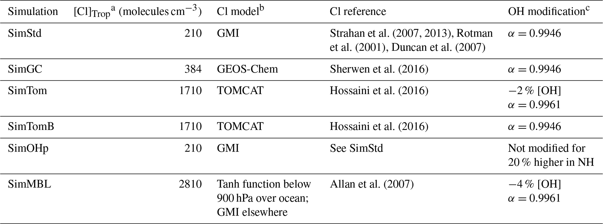
Our standard simulation (SimStd) uses Cl from the GMI CTM for the tropospheric as well as stratospheric loss of CH4 by reaction with Cl. Tropospheric Cl concentrations are small in GMI since it does not include very short lived species, and reaction with Cl represents only 0.28 % of the total tropospheric CH4 loss. We also conduct several sensitivity simulations in which we alter the tropospheric and lower stratospheric Cl fields (Table 2). Cl is not altered above 56 hPa. Sensitivity simulation SimGC uses Cl from the GEOS-Chem chemistry module within GEOS (Long et al., 2015; Hu et al., 2018). GEOS-Chem v11-02f with fully coupled tropospheric and stratospheric chemistry was used for this simulation, with halogen chemistry as described in Sherwen et al. (2016). SimGC has higher values of tropospheric Cl than SimStd (Figs. 3, 4) and leads to 0.66 % of the total CH4 loss occurring via Cl. Both SimStd and SimGC are thus below the 1 % loss via Cl suggested by Gromov et al. (2018). We conduct a third sensitivity simulation, SimTom, which uses Cl from the TOMCAT model simulations that include chlorine sources from chlorocarbons (including very short lived substances), HCl from industry and biomass burning, and very short lived substances (Hossaini et al., 2016). This simulation leads to Cl accounting for 2.5 % of tropospheric CH4 loss in our simulation. Finally, we conduct a fourth sensitivity simulation, SimMBL, which modifies the Cl over the oceans at altitudes below 900 hPa (Fig. 2d) to reflect the marine boundary layer distribution suggested by Allan et al. (2007). This Cl field is described by the following equation:
where λ is latitude in radians and t is the day of the year. Elsewhere SimMBL uses the Cl field from SimStd. This simulation has the highest percent of CH4 loss occurring via Cl: 3.9 %. If we consider the loss of methane throughout the atmosphere rather than just the troposphere, then the percent lost via Cl increases to 1.6 %, 2.0 %, 3.6 %, and 5.0 % for SimStd, SimGC, SimTom, and SimMBL, respectively.
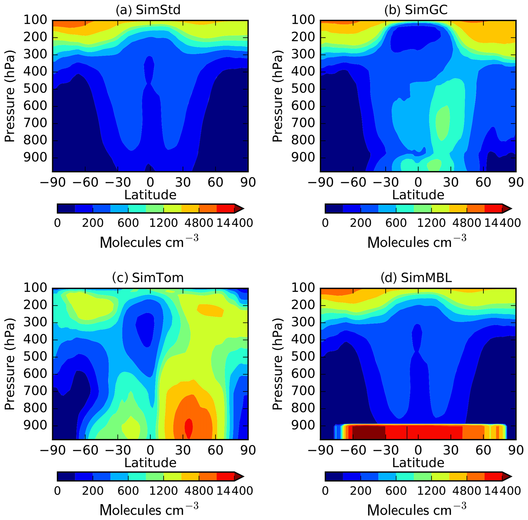
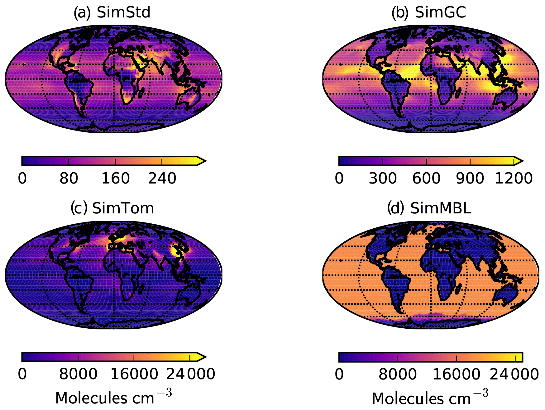
Figure 3Annual mean surface concentrations of Cl in (a) SimStd, (b) SimGC, (c) SimTom, and (d) SimMBL. Note the different color scales between panels.
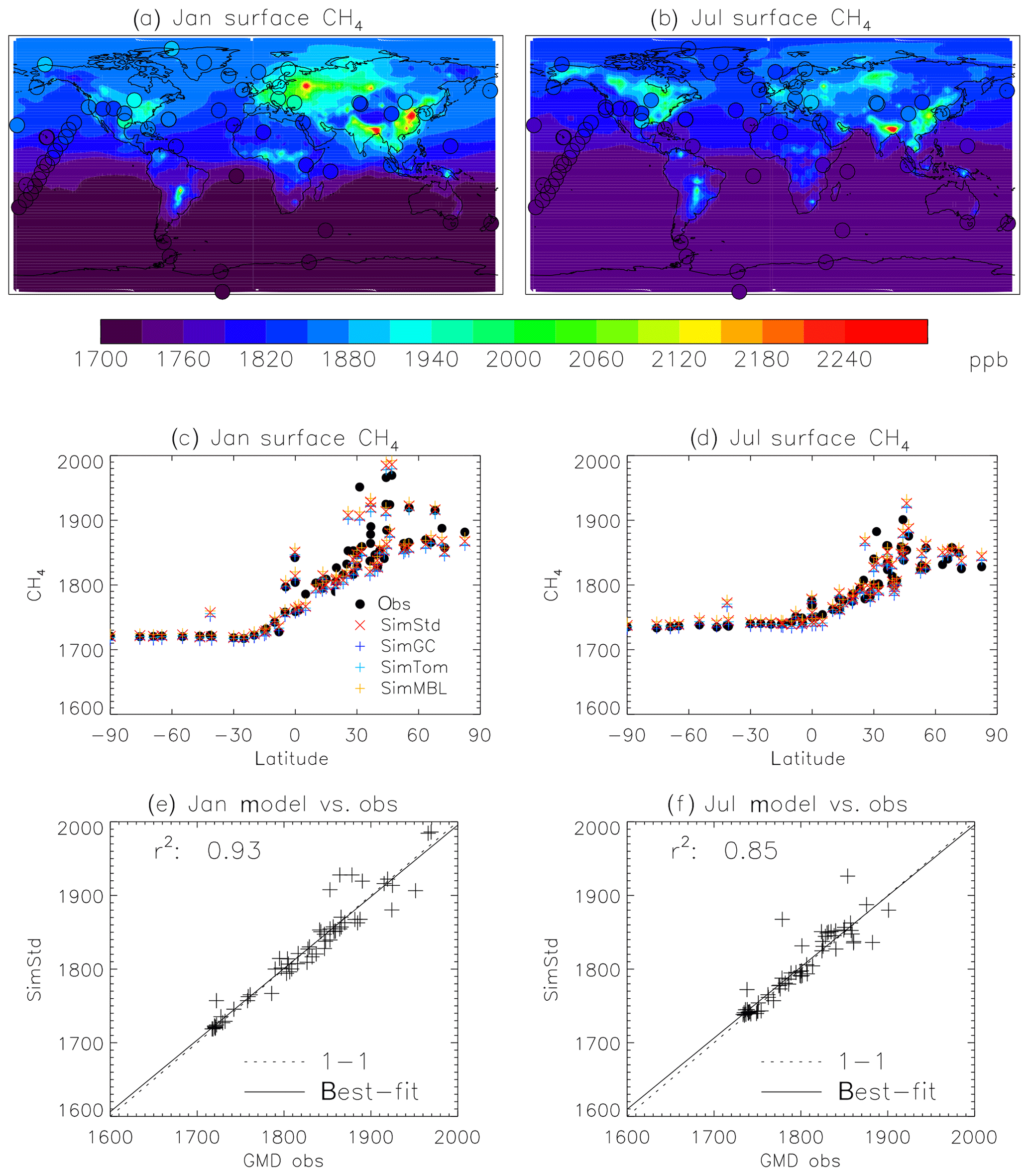
Figure 4Comparison of 2004 simulated and observed surface CH4 concentrations for January (a, c, e) and July (b, d, f). (a, b) Surface concentrations of CH4 from SimStd are overplotted with the concentrations from the GMD observations in circles. (c, d) GMD observations (black circles), SimStd (red ×), SimGC (dark blue +), SimTom (light blue +), and SimMBL (orange +) CH4 as a function of latitude. (e, f) SimStd CH4 (ppb) at the observation locations versus the GMD observations (+ signs) as well as the regression line (solid) and one-to-one line (dashed).
Table 2Oxidants for the standard and sensitivity simulations.
a Concentration of Cl averaged over the troposphere. b Name of the model that generated the offline Cl field. c Changes to [OH] or αOH compared to SimStd.
We designed the sensitivity experiments to alter the isotopic composition of CH4 without greatly affecting the total CH4. Consequently, we reduce the OH concentrations in the SimTom and SimMBL simulations by 2 % and 4 %, respectively, relative to the SimStd OH to offset the effect of increasing Cl. These changes are small compared to the uncertainty in global OH (Rigby et al., 2017). In addition, the SimTom and SimMBL simulations use αOH=0.9961 (Saueressig et al., 2001) rather than αOH=0.9946 (Cantrell et al., 1990) to avoid too much fractionation from the combined Cl and OH sinks. While these changes are necessary to maintain consistent total CH4 and reasonable isotopic ratios, changing multiple factors in addition to Cl makes it difficult to quantify the impact of Cl alone. Consequently, we conduct an additional sensitivity study, called SimTomB, which uses the same Cl field as SimTom but retains the OH and αOH values of SimStd. SimTomB is used in Sect. 3.3. This simulation becomes too heavy compared to observations, justifying the need to change αOH in the main SimTom simulation. We also conduct a sensitivity simulation, SimOHp, that uses the same Cl field as SimStd but does not alter the hemispheric ratio of OH. Table 2 summarizes the standard and sensitivity simulations.
The four Cl distributions differ in their vertical and horizontal spatial distributions as well as their tropospheric mean (Figs. 2 and 3). The SimStd Cl is largest in the tropics, is nearly symmetric between hemispheres, and increases with altitude. Both SimGC and SimTom have Cl that is larger in the Northern Hemisphere than the Southern Hemisphere in the annual mean and reaches a minimum in the midtroposphere. However, the maximum in lower tropospheric Cl occurs in the tropics in SimGC but in the extratropics in SimTom. This midlatitude Cl maximum arises because SimTom has high Cl values over east Asia, whereas SimGC Cl is highest over ocean regions (Fig. 3). SimMBL has a strong maximum in the MBL compared to the free troposphere and land regions. Its annual mean Cl concentrations are higher in the Southern Hemisphere (Fig. 2) due to the larger ocean area in the Southern Hemisphere. However, SimMBL includes a strong seasonal shift in peak Cl between the hemispheres. SimStd and SimGC have more modest seasonal shifts, while Cl in SimTom remains concentrated in the Northern Hemisphere throughout the year (Fig. S3). All simulations repeat the same Cl field from year to year.
The sensitivity simulations listed above are designed to test the role of the Cl sink. We conduct an additional sensitivity study, SimWet, to illustrate the role of spatial variation in the isotopic source signature. SimWet parallels SimStd, but the isotopic composition of the wetland source uses spatial variation from Ganesan et al. (2018). The global mean source signature of the wetland emissions remains −60 ‰.
2.3 Observations
We use surface observations from the NOAA GMD Carbon Cycle Cooperative Global Air Sampling Network to evaluate our simulations. We use the monthly mean observations of total CH4 (Dlugokencky et al., 2018) and δ13C of CH4 (White et al., 2018) to compare to the monthly mean simulation results. The isotopic measurements were made at the Institute of Arctic and Alpine Research at the University of Colorado and are referenced to the VPDB scale (Zhang and Li, 1990). The analytical uncertainty of the isotopic measurements is 0.06 ‰. The variability between measurements taken in a given month may, however, be larger, so we use the maximum of analytical uncertainty and the within-month standard deviation as the uncertainty in the monthly mean. When multiple years of observations are averaged together, we use the pooled variance to calculate the standard error, thus reducing the error based on the number of years. The GMD observations are located at remote sites, shown in Fig. 4 for CH4 in 2004. Measurements of δ13C of CH4 are available at a subset of the sites, shown in Fig. 5.
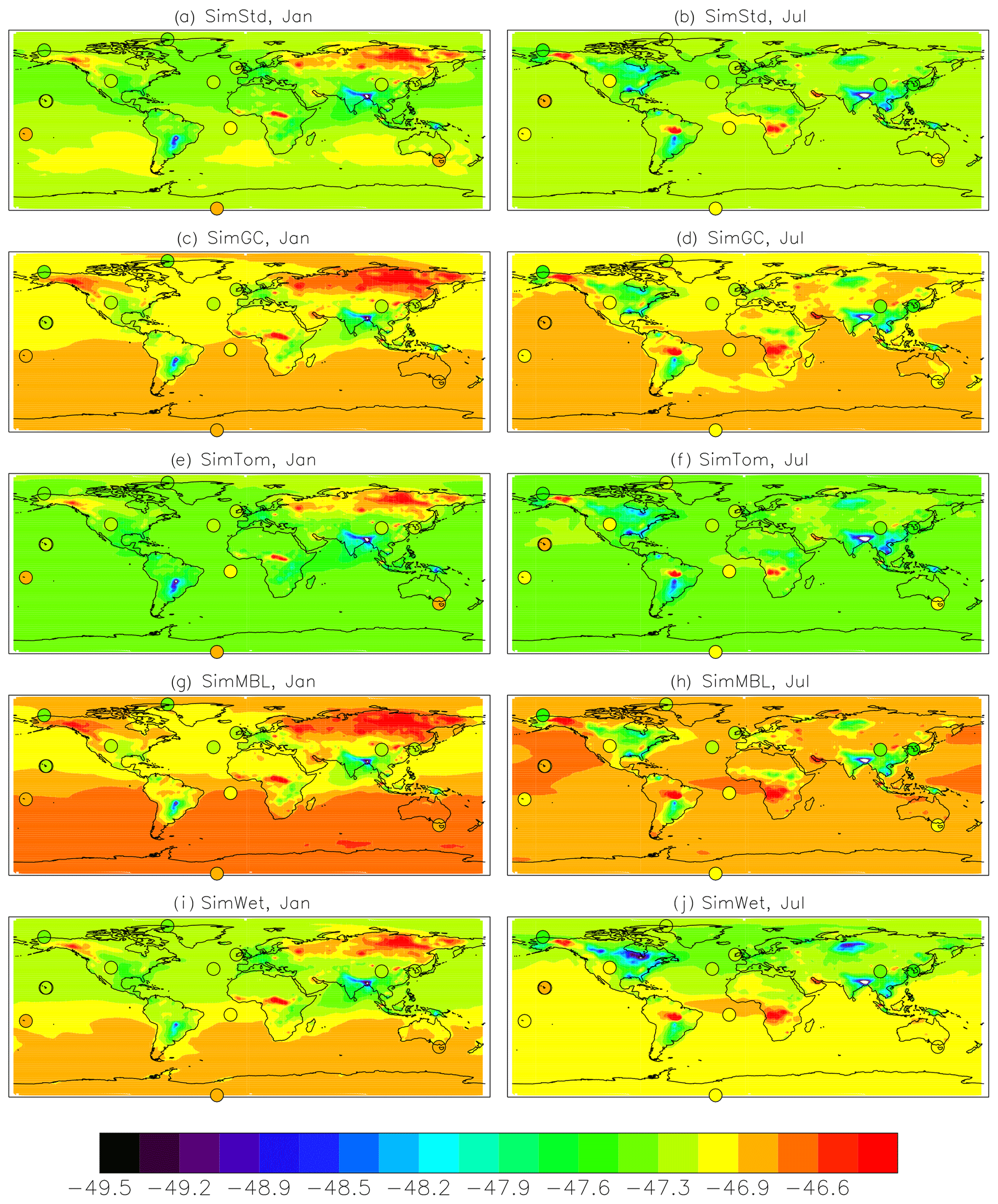
Figure 5Maps of the simulated surface δ13C of CH4 in per mil for January (left) and July (right) overplotted with observations from the GMD sites (circles). The simulations are (a, b) SimStd, (c, d) SimGC, (e, f) SimTom, (g, h) SimMBL, and (i, j) SimWet.
3.1 Evaluation of simulated CH4
We find good agreement between the SimStd simulation and the GMD observations for CH4 (Fig. 4) for 2004. We focus on these 2 months to represent the seasonal differences. The latitudinal distribution is well reproduced, and the simulation captures the elevated concentrations of CH4 observed over Europe in January as well as the January versus July differences in concentration. Overall, the spatial correlation between SimStd and the observations is 0.93 in January and 0.85 in July. The sensitivity simulations described in Table 2 have little effect on the CH4 distribution, as shown by the overlapping symbols in Fig. 4c, d.
3.2 Impact of Cl on the δ13C distribution
We next examine the distribution of δ13C in SimStd compared to observations. Figure 6 shows the time series of observed and simulated δ13C for 1998–2004 at the six GMD sites with δ13C records covering this time period. We begin the figure at 1998 rather than 1990 due to the lack of data availability in the earlier years. The standard and sensitivity simulations overestimate δ13C at the northernmost station, BRW. The observations at the other stations lie within the range of simulations, with most simulations underestimating the observations at the south pole. The differences between the different sensitivity simulations are large compared to the interannual variability in both observed and simulated δ13C. We focus our subsequent analysis on a single year, 2004.
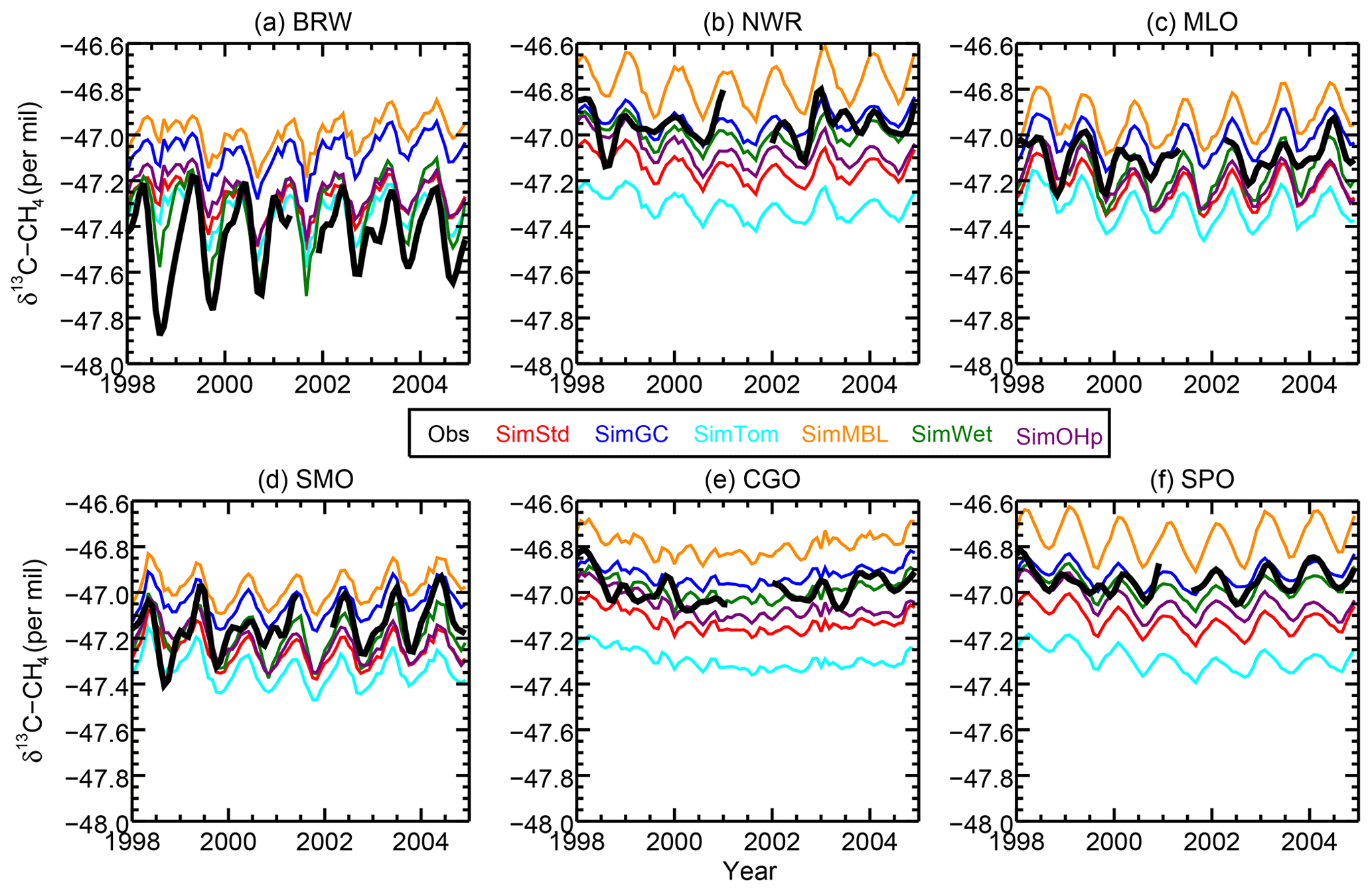
Figure 6The time series of observed (black) and simulated (colors) δ13CH4 at the six GMD sites with records extending back to 1998. BRW: 71.3∘ N, 156.6∘ W; NWR: 40.0∘ N, 105.6∘ W; MLO: 19.5∘ N, 155.6∘ W; CGO: 40.7∘ S, 144.7∘ E; and SPO: 90.0∘ S, 24.8∘ W.
Figure 5a and b show both meridional and zonal variability in δ13C. Background values are less negative (heavier) in the Southern versus Northern Hemisphere (NH) (Fig. 7), a feature seen more strongly in the observations, but there is also variability due to the different source signatures. Areas of biomass burning, such as tropical Africa, show up as particularly heavy, while regions with large wetland and rice emissions, such as SE Asia, are particularly light. Another prominent feature is the isotopically heavy region in northern Eurasia (around 60∘ N) in January, which we attribute to the influence of the geologic (including oil, gas, and coal) source in this region (Fig. S2). This signal is less evident in July, when greater influence from boreal wetlands lightens the isotopic mix. The spatial correlation (r2) between the SimStd and observed δ13C is 0.61 in January and 0.75 in July.

Figure 7δ13C of CH4 as a function of latitude in (a) January and (b) July 2004 for the GMD observations (black circles), SimStd (red), SimGC (dark blue), SimTom (cyan), SimMBL (orange), SimWet (green), and SimOHp (purple). Error bars represent the maximum of the analytical uncertainty (0.06 ‰) and the standard deviation of individual measurements in the month for each site. The colored lines represent the simulated zonal mean, while the colored symbols represent the simulation sampled at the location of the GMD observations.
The sensitivity simulations with altered oxidant concentrations alter the global values of δ13C, but the geographic patterns remain similar to that of SimStd. The larger Cl sink in SimGC leads to an overall less negative δ13C, which agrees better than SimStd with observations at Southern Hemisphere (SH) sites but worse in the NH (Figs. 6c, d and 7). The isotopic effect of the larger Cl sink in SimTom is compensated for by the lower OH and αOH values used in that simulation, flattening the interhemispheric gradient (Figs. 6e, f and 7). In contrast, the very large MBL Cl concentrations in SimMBL lead to an overestimate (insufficiently negative) of the observed δ13C (Fig. 5g, h) but strengthen the interhemispheric gradient. We note that since all simulations began with the same initial conditions but have different sinks, the isotopic composition is not in steady state in 2004 and the results of the sensitivity simulations diverge further with additional years of simulation, with SimMBL becoming clearly inconsistent with observations. We note that while these results highlight the differences in δ13C imposed by changing Cl, the absolute values of δ13C, and hence their agreement with observations, would be different for CH4 source mixtures with a different average δ13C.
Figure 7 reveals an underestimate in the interhemispheric gradient of δ13C in both SimStd and the sensitivity runs compared to the GMD observations. Table 3 presents the observed and simulated δ13C interhemispheric gradients calculated as the difference between the δ13C values averaged over all sites south of 30∘ S and the average over sites north of 30∘ N. SimStd and SimGC show similar underestimates of the observed gradient, and the underestimate is more severe in SimTom. The gradient is improved in SimMBL in January. The differences between simulations reflect differences in the locations where CH4 oxidation occurs and the amount and location of isotopic fractionation due to Cl versus OH. Figure 8 shows that the higher Cl values over the NH, particularly China, in SimTom versus SimStd lead to more CH4 loss occurring in the NH and higher (heavier) δ13C in the NH. This effect is particularly pronounced over China and Europe. Less fractionation by the OH sink in SimTom leads to lighter values in the SH. Conversely, SimMBL has more loss occurring over the SH oceans in January, leading to heavier δ13C in the SH (Fig. 9). This effect is not present in July, when the SimMBL Cl loss shifts to the NH (Fig. S4). The reduced hemispheric difference in OH in SimOHp leads to a small improvement in the hemispheric gradient in δ13C.
Table 3Observed and simulated interhemispheric gradient in δ13C-CH4.

* Average δ13C-CH4 at GMD site locations south of 30∘ S minus average δ13C-CH4 at locations north of 30∘ N.
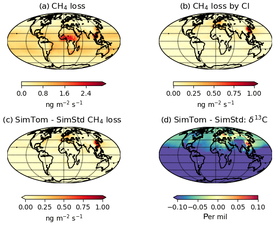
Figure 8January (a) CH4 loss and (b) CH4 loss by Cl only in the SimTom simulation, as well as the difference in (c) CH4 loss and (d) δ13C-CH4 between the SimTom and SimStd simulations.

Figure 9January (a) CH4 loss and (b) CH4 loss by Cl only in the SimMBL simulation, as well as the difference in (c) CH4 loss and (d) δ13C-CH4 between the SimMBL and SimStd simulations.
We further examine the seasonal cycle of δ13C in Fig. 10. We focus on the seasonal cycle at the South Pole Observatory (SPO) site because it is far from large CH4 sources, and thus the seasonal cycle depends strongly on the seasonality of the CH4 sinks. While all simulations lie mostly within the error bars of the observations, SimMBL has the largest seasonal cycle amplitude, overestimating the seasonal cycle at of the SPO observations with a δ13C value that is both too heavy in February–June and too light in August–November. In contrast, SimStd and the other sensitivity simulations underestimate the magnitude of the observed seasonal cycle at SPO. Figure S5 shows a large enhancement in the seasonal cycle amplitude between SimMBL and the other simulations for the Cape Grim site in Tasmania (CGO) but only a small change at other sites. This suggests that while MBL Cl is attractive as an explanation for the SH seasonality of δ13C, this explanation may be inconsistent with the inclusion of nonmarine Cl sources. However, since the seasonal cycle amplitude at SPO lies in between SimMBL and the other simulations, it is possible that at an MBL Cl source similar to that of SimMBL but with a smaller average value could reproduce the amplitude well.
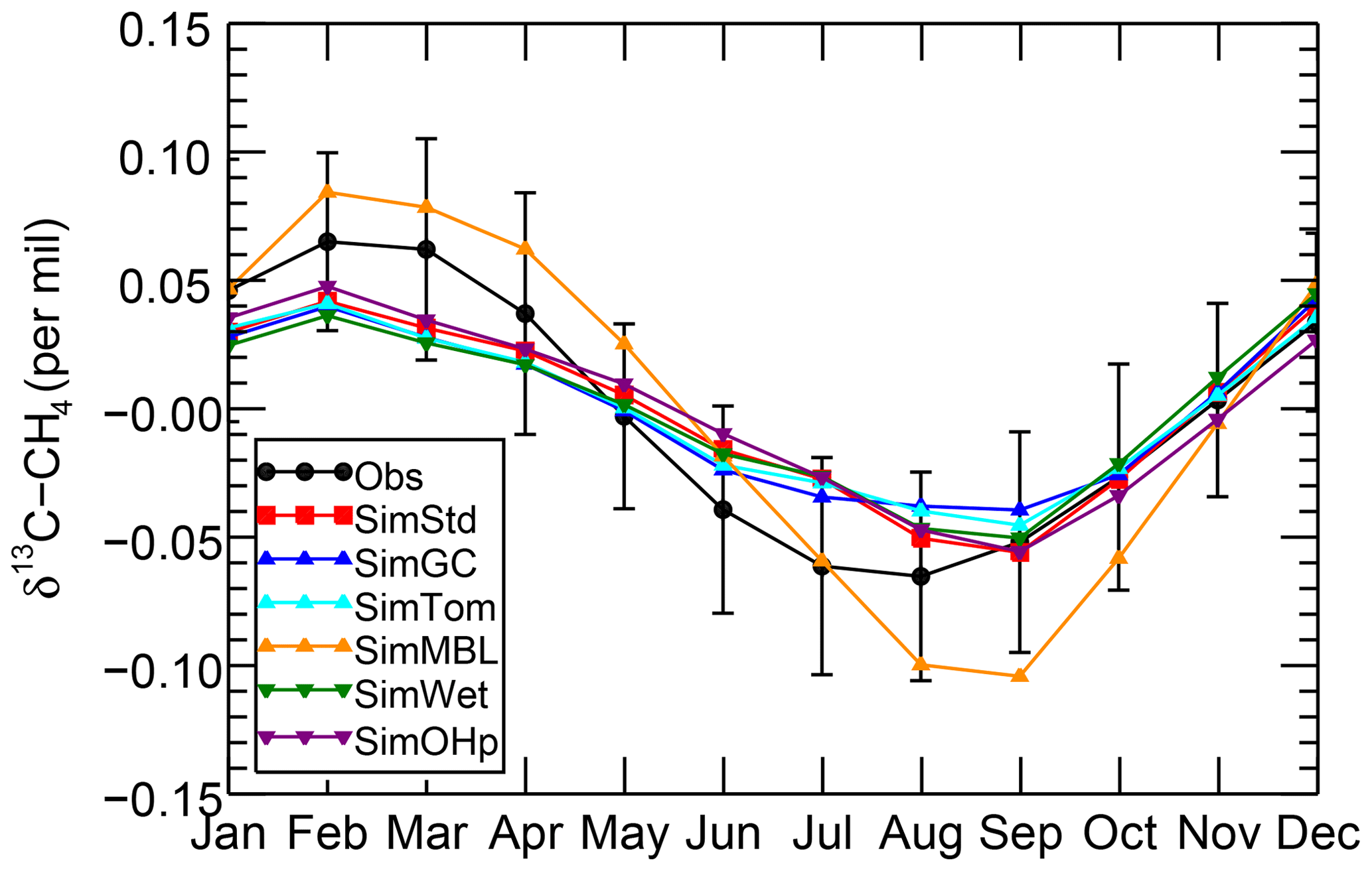
Figure 10The seasonal cycle of δ13C of CH4 at the SPO site with the annual mean removed averaged over 2002–2004 for the GMD observations (black), SimStd (red), SimGC (blue), SimTom (cyan), SimMBL (orange), SimWet (green), and SimOHp (purple). Error bars represent the standard error, calculated as the maximum of the pooled standard deviation or the analytical uncertainty (0.06 ‰), divided by the square root of the number of years of observations.
3.3 Quantifying the sensitivity of δ13C to CH4 loss by Cl
Given the substantial range in estimates for how much methane is lost by reaction with tropospheric Cl, it is important to quantify the sensitivity of global mean surface δ13C to the CH4 loss by Cl. This analysis summarizes the global impact of the isotopic effect of the Cl differences between simulations discussed above. Figure 11 shows the global mean, area-weighted surface δ13C in 2004 as a function of the percent of CH4 oxidized by Cl for SimStd, SimGC, and SimTomB, the three simulations with the same OH and emissions but different Cl. A strong linear relationship is evident between the oxidation by Cl and the surface δ13C. The slope of the linear regression line indicates the expected increase in surface δ13C for a change in the percent of CH4 oxidized by Cl. Based on this analysis we expect that surface δ13C will increase by approximately 0.5 ‰ for each percent increase in CH4 loss by Cl.
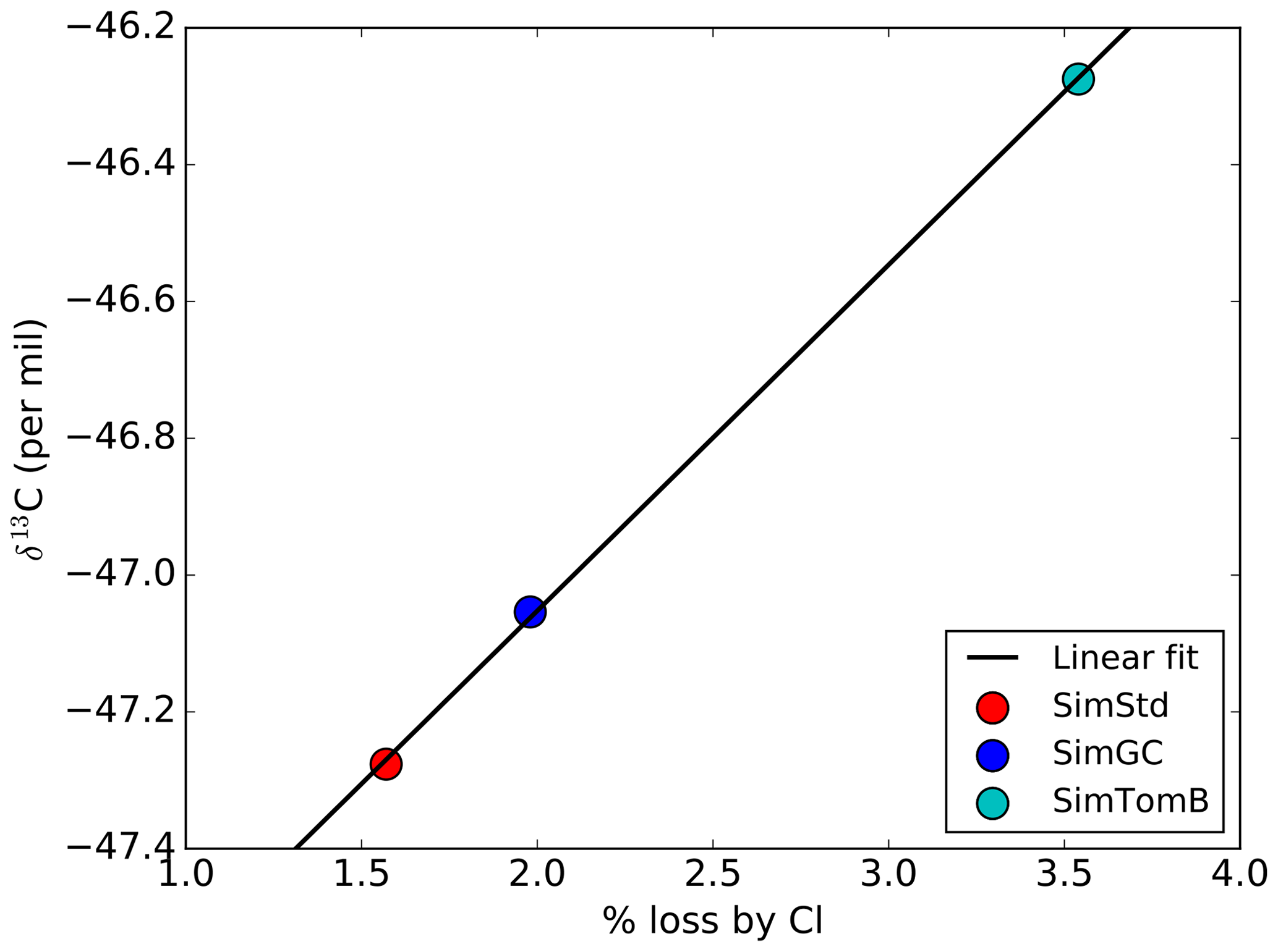
Figure 11Area-weighted global mean surface δ13C for the SimStd (red), SimGC (blue), and SimTomB (cyan) simulations in 2004 as a function of the percent of CH4 loss occurring by reaction with Cl. The linear best-fit line is shown in black.
3.4 Sensitivity of δ13C to the isotopic distribution of sources
Other factors in addition to the Cl distribution likely contribute to the mismatch between the observed and simulated interhemispheric gradients. Figure 5 shows the impact of the geologic source on the δ13C values over northern Asia. A bias in either the strength or the isotopic composition of this source will impact the interhemispheric gradient. Another likely contributing factor is our use of a globally uniform isotopic ratio for each source type. Ganesan et al. (2018) developed a global map of the isotopic signatures of wetland emissions. We use this map to impose spatially varying isotopic ratios on our SimWet simulation. SimWet increases the amplitude of the seasonal cycle in δ13C-CH4 particularly for northern latitudes sites such as ALT, BRW, and MHD (Fig. S5). It has little effect on the seasonal cycle at the SH CGO and SPO sites, where SimMBL shows a large effect on the cycle. SimWet results in improved agreement with the observed interhemispheric gradient (Figs. 5, 7; Table 3). SimWet is better able to simultaneously match the δ13C-CH4 observations at both the northernmost (BRW) and southernmost (SPO) sites shown in Fig. 6 than the other simulations, even though all simulations reproduce the latitudinal distribution of CH4 well (Fig. 4). This highlights the importance of spatially varying isotopic ratios for the δ13C-CH4 distribution. The size of the effect of including spatially varying ratios in wetland emissions depends on the strength of the wetland emissions as well as the other sources. Including spatially varying isotopic signature for other sources as well could further modify the simulated interhemispheric gradient, potentially correcting some of the flat gradient of, e.g., the SimTom simulation.
The role of Cl as a methane sink is a significant uncertainty in the global CH4 budget, particularly with respect to isotopes. The global distribution of Cl is not well known from observations, and the Cl distributions simulated by global models vary widely from model to model. We investigated the sensitivity of the surface δ13C distribution of CH4 to the intermodel diversity in tropospheric Cl using a series of sensitivity studies with a global 3D model. Given the uncertainties in CH4 sources and their isotopic ratios, it is not possible to conclude from this study which Cl field is best. However, the differences between the simulations provide insight on the strong lever that tropospheric Cl exerts on the δ13C distribution.
Our standard and sensitivity simulations all reproduce well the geographic distribution of and temporal evolution of CH4 observed at the GMD surface sites. However, imposing Cl distributions from a range of chemical transport models used in the scientific community leads to large differences in the simulated distribution of the δ13C of CH4. The CH4 sinks from Cl in our SimStd and SimGC simulations are both below 1 % of the total CH4 sink, as suggested by Gromov et al. (2018). Yet the SimStd and SimGC simulations underestimate and overestimate, respectively, the observed δ13C in 2004, despite the fact that both include only a relatively small CH4 sink from Cl.
Our ability to reproduce the observed latitudinal distribution of δ13C depends not only on the assumed value of global mean Cl, but also its geographic distribution. The detailed halogen chemistry model (TOMCAT) of Hossaini et al. (2016) places the maximum Cl values in the continental NH, in contrast to the large MBL Cl sink used in Allan et al. (2007) to explain SH observations. We find that the strong NH Cl maximum, along with the resulting reduction in OH fractionation required to maintain consistency with observations, acts to flatten the interhemispheric gradient of δ13C, while the MBL Cl sink increases the hemispheric differences in NH winter and also strengthens the seasonal cycle. However, the interhemispheric gradient is also influenced by spatial variation in the isotopic signatures of the sources and uncertainties in the soil sink, complicating this issue.
Two values for the fractionating effect of OH (αOH) on δ13C (Cantrell et al., 1990; Saueressig et al., 2001) are widely cited in the literature. Combining the TOMCAT Cl fields with the αOH of Saueressig et al. (2001) leads to an underestimate of observed δ13C, but combining it with the Cantrell et al. (1990) αOH would lead to an overestimate. Reducing uncertainty in the fractionating effect of OH would thus improve our ability to constrain the role of Cl.
Observations of the δ13C of CH4 provide an important tool for constraining the CH4 budget. We find that the range of Cl fields available from current global models leads to a wide range of simulated δ13C values. Each percent increase in the amount of CH4 loss occurring by reaction with Cl increases global mean surface δ13C of CH4 by approximately 0.5 ‰. This relationship can be used to estimate the impact on methane's isotopic values from future model simulations of Cl. The choice of Cl field thus strongly impacts what CH4 source mixture best fits δ13C observations. Better quantification of the role of Cl in the methane budget and further developing models of tropospheric halogens are therefore critical for interpreting the δ13C observations to their fullest potential.
The methane (Dlugokencky et al., 2018) and δ13CH4 (White et al., 2018) observations are available from the NOAA GMD website: https://www.esrl.noaa.gov/gmd/dv/data/ (Global Monitoring Laboratory, 2020). Output from the GEOS model is on the NASA Center for Climate Simulation (NCCS) system.
The supplement related to this article is available online at: https://doi.org/10.5194/acp-20-8405-2020-supplement.
SAS designed and conducted the simulations, performed the analysis, and prepared the manuscript. JSW contributed to model development and experiment design. MM contributed to model development. BD contributed to model development and conceptualization. RH and CAK contributed inputs to the simulations. SEM and JWCW contributed data and aided in their interpretation. All authors contributed to the editing and revising of the manuscript.
The authors declare that they have no conflict of interest.
Computational resources were provided by the NASA Center for Climate Simulation (NCCS). The authors thank Prabir Patra for useful discussions. Ryan Hossaini is supported by a NERC Independent Research Fellowship (NE/N014375/1).
This paper was edited by Patrick Jöckel and reviewed by two anonymous referees.
Allan, W., Manning, M. R., Lassey, K. R., Lowe, D. C., and Gomez, A. J.: Modeling the variation of δ13C in atmospheric methane: Phase ellipses and the kinetic isotope effect, Global Biogeochem. Cy., 15, 467–481, https://doi.org/10.1029/2000GB001282, 2001.
Allan, W., Struthers, H., and Lowe, D.: Methane carbon isotope effects caused by atomic chlorine in the marine boundary layer: Global model results compared with Southern Hemisphere measurements, J. Geophys. Res.-Atmos., 112, D04306, https://doi.org/10.1029/2006JD007369, 2007.
Bock, M., Schmitt, J., Beck, J., Seth, B., Chappellaz, J., and Fischer, H.: Glacial/interglacial wetland, biomass burning, and geologic methane emissions constrained by dual stable isotopic CH4 ice core records, P. Natl. Acad. Sci. USA, 114, E5778–E5786, https://doi.org/10.1073/pnas.1613883114, 2017.
Brownlow, R., Lowry, D., Fisher, R., France, J., Lanoisellé, M., White, B., Wooster, M., Zhang, T., and Nisbet, E.: Isotopic ratios of tropical methane emissions by atmospheric measurement, Global Biogeochem. Cy., 31, 1408–1419, 2017.
Cantrell, C. A., Shetter, R. E., McDaniel, A. H., Calvert, J. G., Davidson, J. A., Lowe, D. C., Tyler, S. C., Cicerone, R. J., and Greenberg, J. P.: Carbon kinetic isotope effect in the oxidation of methane by the hydroxyl radical, J. Geophys. Res.-Atmos., 95, 22455–22462, 1990.
Craig, H.: Isotopic Standards for Carbon and Oxygen and Correction Factors for Mass-Spectrometric Analysis OF Carbon Dioxide, Geochim. Cosmochim. Ac., 12, 133–149, https://doi.org/10.1016/0016-7037(57)90024-8, 1957.
Dlugokencky, E., Bruhwiler, L., White, J., Emmons, L., Novelli, P., Montzka, S., Masarie, K., Lang, P., Crotwell, A., Miller, J., and Gatti, L.: Observational constraints on recent increases in the atmospheric CH4 burden, Geophys. Res. Lett., 36, L18803, https://doi.org/10.1029/2009GL039780, 2009.
Dlugokencky, E., Nisbet, E., Fisher, R., and Lowry, D.: Global atmospheric methane: budget, changes and dangers, Philos. T. R. Soc. A, 369, 2058–2072, https://doi.org/10.1098/rsta.2010.0341, 2011.
Dlugokencky, E. J., Lang, P. M., Crotwell, A. M., Mund, J. W., Crotwell, M. J., and Thoning, K. W.: Atmospheric Methane Dry Air Mole Fractions from the NOAA ESRL Carbon Cycle Cooperative Global Air Sampling Network, 1983–2017, Version: 2018-08-01, available at: ftp://aftp.cmdl.noaa.gov/data/trace_gases/ch4/flask/surface/ (last access: 30 January 2019), 2018.
Duncan, B. N., Strahan, S. E., Yoshida, Y., Steenrod, S. D., and Livesey, N.: Model study of the cross-tropopause transport of biomass burning pollution, Atmos. Chem. Phys., 7, 3713–3736, https://doi.org/10.5194/acp-7-3713-2007, 2007.
Elshorbany, Y. F., Duncan, B. N., Strode, S. A., Wang, J. S., and Kouatchou, J.: The description and validation of the computationally Efficient CH4–CO–OH (ECCOHv1.01) chemistry module for 3-D model applications, Geosci. Model Dev., 9, 799–822, https://doi.org/10.5194/gmd-9-799-2016, 2016.
Etiope, G. and Milkov, A.: A new estimate of global methane flux from onshore and shallow submarine mud volcanoes to the atmosphere, Environ. Geol., 46, 997–1002, https://doi.org/10.1007/s00254-004-1085-1, 2004.
European Commission: Joint Research Center (JRC)/Netherlands Environmental Assessment Agency (PBL), Emission Database for Global Atmospheric Research (EDGAR), available at: http://edgar.jrc.ec.europe.eu (last access: 6 July 2016), 2011.
Ferretti, D. F., Miller, J. B., White, J. W. C., Etheridge, D. M., Lassey, K. R., Lowe, D. C., Meure, C. M. M., Dreier, M. F., Trudinger, C. M., van Ommen, T. D., and Langenfelds, R. L.: Unexpected Changes to the Global Methane Budget over the Past 2000 Years, Science, 309, 1714–1717, https://doi.org/10.1126/science.1115193, 2005.
Fischer, H., Behrens, M., Bock, M., Richter, U., Schmitt, J., Loulergue, L., Chappellaz, J., Spahni, R., Blunier, T., Leuenberger, M., and Stocker, T. F.: Changing boreal methane sources and constant biomass burning during the last termination, Nature, 452, 864, https://doi.org/10.1038/nature06825, 2008.
Fung, I., John, J., Lerner, J., Matthews, E., Prather, M., Steele, L., and Fraser, P.: 3-Dimensional Model Synthesis of the Global Methane Cycle, J. Geophys. Res.-Atmos., 96, 13033–13065, https://doi.org/10.1029/91JD01247, 1991.
Ganesan, A., Stell, A., Gedney, N., Comyn-Platt, E., Hayman, G., Rigby, M., Poulter, B., and Hornibrook, E.: Spatially Resolved Isotopic Source Signatures of Wetland Methane Emissions, Geophys. Res. Lett., 45, 3737–3745, 2018.
Gelaro, R., McCarty, W., Suarez, M., Todling, R., Molod, A., Takacs, L., Randles, C., Darmenov, A., Bosilovich, M., Reichle, R., Wargan, K., Coy, L., Cullather, R., Draper, C., Akella, S., Buchard, V., Conaty, A., da Silva, A., Gu, W., Kim, G., Koster, R., Lucchesi, R., Merkova, D., Nielsen, J., Partyka, G., Pawson, S., Putman, W., Rienecker, M., Schubert, S., Sienkiewicz, M., and Zhao, B.: The Modern-Era Retrospective Analysis for Research and Applications, Version 2 (MERRA-2), J. Climate, 30, 5419–5454, https://doi.org/10.1175/JCLI-D-16-0758.1, 2017.
Ghosh, A., Patra, P. K., Ishijima, K., Umezawa, T., Ito, A., Etheridge, D. M., Sugawara, S., Kawamura, K., Miller, J. B., Dlugokencky, E. J., Krummel, P. B., Fraser, P. J., Steele, L. P., Langenfelds, R. L., Trudinger, C. M., White, J. W. C., Vaughn, B., Saeki, T., Aoki, S., and Nakazawa, T.: Variations in global methane sources and sinks during 1910–2010, Atmos. Chem. Phys., 15, 2595–2612, https://doi.org/10.5194/acp-15-2595-2015, 2015.
Global Monitoring Laboratory: GML Data Finder, available at: https://www.esrl.noaa.gov/gmd/dv/data/, last access: 13 July 2020.
Granier, C., Bessagnet, B., Bond, T., D'Angiola, A., van der Gon, H. D., Frost, G. J., Heil, A., Kaiser, J. W., Kinne, S., Klimont, Z., Kloster, S., Lamarque, J. F., Liousse, C., Masui, T., Meleux, F., Mieville, A., Ohara, T., Raut, J. C., Riahi, K., Schultz, M. G., Smith, S. J., Thompson, A., van Aardenne, J., van der Werf, G. R., and van Vuuren, D. P.: Evolution of anthropogenic and biomass burning emissions of air pollutants at global and regional scales during the 1980-2010 period, Climatic Change, 109, 163–190, https://doi.org/10.1007/s10584-011-0154-1, 2011.
Gromov, S., Brenninkmeijer, C. A. M., and Jöckel, P.: A very limited role of tropospheric chlorine as a sink of the greenhouse gas methane, Atmos. Chem. Phys., 18, 9831–9843, https://doi.org/10.5194/acp-18-9831-2018, 2018.
Hausmann, P., Sussmann, R., and Smale, D.: Contribution of oil and natural gas production to renewed increase in atmospheric methane (2007–2014): top–down estimate from ethane and methane column observations, Atmos. Chem. Phys., 16, 3227–3244, https://doi.org/10.5194/acp-16-3227-2016, 2016.
Hopcroft, P. O., Valdes, P. J., and Kaplan, J. O.: Bayesian Analysis of the Glacial-Interglacial Methane Increase Constrained by Stable Isotopes and Earth System Modeling, Geophys. Res. Lett., 45, 3653–3663, https://doi.org/10.1002/2018GL077382, 2018.
Hossaini, R., Chipperfield, M. P., Saiz-Lopez, A., Fernandez, R., Monks, S., Feng, W., Brauer, P., and von Glasow, R.: A global model of tropospheric chlorine chemistry: Organic versus inorganic sources and impact on methane oxidation, J. Geophys. Res.-Atmos., 121, 14271–14297, https://doi.org/10.1002/2016JD025756, 2016.
Houweling, S., Kaminski, T., Dentener, F., Lelieveld, J., and Heimann, M.: Inverse modeling of methane sources and sinks using the adjoint of a global transport model, J. Geophys. Res.-Atmos., 104, 26137–26160, https://doi.org/10.1029/1999JD900428, 1999.
Houweling, S., Dentener, F., and Lelieveld, J.: Simulation of preindustrial atmospheric methane to constrain the global source strength of natural wetlands, J. Geophys. Res.-Atmos., 105, 17243–17255, https://doi.org/10.1029/2000JD900193, 2000.
Houweling, S., Van der Werf, G., Goldewijk, K. K., Röckmann, T., and Aben, I.: Early anthropogenic CH4 emissions and the variation of CH4 and 13CH4 over the last millennium, Global Biogeochem. Cy., 22, GB1002, https://doi.org/10.1029/2007GB002961, 2008.
Hu, L., Keller, C. A., Long, M. S., Sherwen, T., Auer, B., Da Silva, A., Nielsen, J. E., Pawson, S., Thompson, M. A., Trayanov, A. L., Travis, K. R., Grange, S. K., Evans, M. J., and Jacob, D. J.: Global simulation of tropospheric chemistry at 12.5 km resolution: performance and evaluation of the GEOS-Chem chemical module (v10-1) within the NASA GEOS Earth system model (GEOS-5 ESM), Geosci. Model Dev., 11, 4603–4620, https://doi.org/10.5194/gmd-11-4603-2018, 2018.
Ito, A. and Inatomi, M.: Use of a process-based model for assessing the methane budgets of global terrestrial ecosystems and evaluation of uncertainty, Biogeosciences, 9, 759–773, https://doi.org/10.5194/bg-9-759-2012, 2012.
Kai, F., Tyler, S., Randerson, J., and Blake, D.: Reduced methane growth rate explained by decreased Northern Hemisphere microbial sources, Nature, 476, 194–197, https://doi.org/10.1038/nature10259, 2011.
Kirschke, S., Bousquet, P., Ciais, P., Saunois, M., Canadell, J. G., Dlugokencky, E. J., Bergamaschi, P., Bergmann, D., Blake, D. R., Bruhwiler, L., Cameron-Smith, P., Castaldi, S., Chevallier, F., Feng, L., Fraser, A., Heimann, M., Hodson, E. L., Houweling, S., Josse, B., Fraser, P. J., Krummel, P. B., Lamarque, J.-F., Langenfelds, R. L., Le Quere, C., Naik, V., O'Doherty, S., Palmer, P. I., Pison, I., Plummer, D., Poulter, B., Prinn, R. G., Rigby, M., Ringeval, B., Santini, M., Schmidt, M., Shindell, D. T., Simpson, I. J., Spahni, R., Steele, L. P., Strode, S. A., Sudo, K., Szopa, S., van der Werf, G. R., Voulgarakis, A., van Weele, M., Weiss, R. F., Williams, J. E., and Zeng, G.: Three decades of global methane sources and sinks, Nat. Geosci., 6, 813–823, https://doi.org/10.1038/NGEO1955, 2013.
Lassey, K. R., Etheridge, D. M., Lowe, D. C., Smith, A. M., and Ferretti, D. F.: Centennial evolution of the atmospheric methane budget: what do the carbon isotopes tell us?, Atmos. Chem. Phys., 7, 2119–2139, https://doi.org/10.5194/acp-7-2119-2007, 2007.
Long, M. S., Yantosca, R., Nielsen, J. E., Keller, C. A., da Silva, A., Sulprizio, M. P., Pawson, S., and Jacob, D. J.: Development of a grid-independent GEOS-Chem chemical transport model (v9-02) as an atmospheric chemistry module for Earth system models, Geosci. Model Dev., 8, 595–602, https://doi.org/10.5194/gmd-8-595-2015, 2015.
McNorton, J., Chipperfield, M. P., Gloor, M., Wilson, C., Feng, W., Hayman, G. D., Rigby, M., Krummel, P. B., O'Doherty, S., Prinn, R. G., Weiss, R. F., Young, D., Dlugokencky, E., and Montzka, S. A.: Role of OH variability in the stalling of the global atmospheric CH4 growth rate from 1999 to 2006, Atmos. Chem. Phys., 16, 7943–7956, https://doi.org/10.5194/acp-16-7943-2016, 2016.
Mikaloff Fletcher, S. E., Tans, P. P., Bruhwiler, L. M., Miller, J. B., and Heimann, M.: CH4 sources estimated from atmospheric observations of CH4 and its 13C∕12C isotopic ratios: 2. Inverse modeling of CH4 fluxes from geographical regions, Global Biogeochem. Cy., 18, GB4005, https://doi.org/10.1029/2004GB002224, 2004a.
Mikaloff Fletcher, S. E., Tans, P. P., Bruhwiler, L. M., Miller, J. B., and Heimann, M.: CH4 sources estimated from atmospheric observations of CH4 and its 13C∕12C isotopic ratios: 1. Inverse modeling of source processes, Global Biogeochem. Cy., 18, GB4004, https://doi.org/10.1029/2004GB002223, 2004b.
Molod, A., Takacs, L., Suarez, M., and Bacmeister, J.: Development of the GEOS-5 atmospheric general circulation model: evolution from MERRA to MERRA2, Geosci. Model Dev., 8, 1339–1356, https://doi.org/10.5194/gmd-8-1339-2015, 2015.
Monteil, G., Houweling, S., Dlugockenky, E. J., Maenhout, G., Vaughn, B. H., White, J. W. C., and Rockmann, T.: Interpreting methane variations in the past two decades using measurements of CH4 mixing ratio and isotopic composition, Atmos. Chem. Phys., 11, 9141–9153, https://doi.org/10.5194/acp-11-9141-2011, 2011.
Naik, V., Voulgarakis, A., Fiore, A. M., Horowitz, L. W., Lamarque, J.-F., Lin, M., Prather, M. J., Young, P. J., Bergmann, D., Cameron-Smith, P. J., Cionni, I., Collins, W. J., Dalsøren, S. B., Doherty, R., Eyring, V., Faluvegi, G., Folberth, G. A., Josse, B., Lee, Y. H., MacKenzie, I. A., Nagashima, T., van Noije, T. P. C., Plummer, D. A., Righi, M., Rumbold, S. T., Skeie, R., Shindell, D. T., Stevenson, D. S., Strode, S., Sudo, K., Szopa, S., and Zeng, G.: Preindustrial to present-day changes in tropospheric hydroxyl radical and methane lifetime from the Atmospheric Chemistry and Climate Model Intercomparison Project (ACCMIP), Atmos. Chem. Phys., 13, 5277–5298, https://doi.org/10.5194/acp-13-5277-2013, 2013.
Nielsen, J., Pawson, S., Molod, A., Auer, B., da Silva, A., Douglass, A., Duncan, B., Liang, Q., Manyin, M., Oman, L., Putman, W., Strahan, S., and Wargan, K.: Chemical Mechanisms and Their Applications in the Goddard Earth Observing System (GEOS) Earth System Model, J. Adv. Model. Earth Sy., 9, 3019–3044, https://doi.org/10.1002/2017MS001011, 2017.
Nisbet, E., Dlugokencky, E., Manning, M., Lowry, D., Fisher, R., France, J., Michel, S., Miller, J., White, J., and Vaughn, B.: Rising atmospheric methane: 2007–2014 growth and isotopic shift, Global Biogeochem. Cy., 30, 1356–1370, 2016.
Nisbet, E., Manning, M., Dlugokencky, E., Fisher, R., Lowry, D., Michel, S., Myhre, C., Platt, M., Allen, G., Bousquet, P., Brownlow, R., Cain, M., France, J., Hermansen, O., Hossaini, R., Jones, A., Levin, I., Manning, A., Myhre, G., Pyle, J., Vaughn, B., Warwick, N., and White, J.: Very Strong. Atmospheric Methane Growth in the 4 Years 2014–2017: Implications for the paris Agreement, Global Biogeochem. Cy., 33, 318–342, https://doi.org/10.1029/2018GB006009, 2019.
Orbe, C., Oman, L., Strahan, S., Waugh, D., Pawson, S., Takacs, L., and Molod, A.: Large-Scale Atmospheric Transport in GEOS Replay Simulations, J. Adv. Model. Earth Sy., 9, 2545–2560, https://doi.org/10.1002/2017MS001053, 2017.
Patra, P. K., Houweling, S., Krol, M., Bousquet, P., Belikov, D., Bergmann, D., Bian, H., Cameron-Smith, P., Chipperfield, M. P., Corbin, K., Fortems-Cheiney, A., Fraser, A., Gloor, E., Hess, P., Ito, A., Kawa, S. R., Law, R. M., Loh, Z., Maksyutov, S., Meng, L., Palmer, P. I., Prinn, R. G., Rigby, M., Saito, R., and Wilson, C.: TransCom model simulations of CH4 and related species: linking transport, surface flux and chemical loss with CH4 variability in the troposphere and lower stratosphere, Atmos. Chem. Phys., 11, 12813–12837, https://doi.org/10.5194/acp-11-12813-2011, 2011.
Platt, U., Allan, W., and Lowe, D.: Hemispheric average Cl atom concentration from 13C∕12C ratios in atmospheric methane, Atmos. Chem. Phys., 4, 2393–2399, https://doi.org/10.5194/acp-4-2393-2004, 2004.
Quay, P., King, S., Stutsman, J., Wilbur, D., Steele, L., Fung, I., Gammon, R., Brown, T., Farwell, G., Grootes, P., and Schmidt, F.: Carbon Isotopic Composition of Atmospheric CH4: Fossil and Biomass Burning Source Strenghts, Global Biogeochem. Cy., 5, 25–47, https://doi.org/10.1029/91GB00003, 1991.
Rice, A. L., Butenhoff, C. L., Teama, D. G., Röger, F. H., Khalil, M. A. K., and Rasmussen, R. A.: Atmospheric methane isotopic record favors fossil sources flat in 1980s and 1990s with recent increase, P. Natl. Acad. Sci. USA, 113, 10791–10796, 2016.
Rigby, M., Prinn, R. G., Fraser, P. J., Simmonds, P. G., Langenfelds, R. L., Huang, J., Cunnold, D. M., Steele, L. P., Krummel, P. B., Weiss, R. F., O'Doherty, S., Salameh, P. K., Wang, H. J., Harth, C. M., Mühle, J., and Porter, L. W.: Renewed growth of atmospheric methane, Geophys. Res. Lett., 35, L22805, https://doi.org/10.1029/2008GL036037, 2008.
Rigby, M., Montzka, S. A., Prinn, R. G., White, J. W., Young, D., O'Doherty, S., Lunt, M. F., Ganesan, A. L., Manning, A. J., and Simmonds, P. G.: Role of atmospheric oxidation in recent methane growth, P. Natl. Acad. Sci. USA, 114, 5373–5377, 2017.
Rotman, D., Tannahill, J., Kinnison, D., Connell, P., Bergmann, D., Proctor, D., Rodriguez, J., Lin, S., Rood, R., Prather, M., Rasch, P., Considine, D., Ramaroson, R., and Kawa, S.: Global Modeling Initiative assessment model: Model description, integration, and testing of the transport shell, J. Geophys. Res.-Atmos., 106, 1669–1691, https://doi.org/10.1029/2000JD900463, 2001.
Saueressig, G., Bergamaschi, P., Crowley, J., Fischer, H., and Harris, G.: Carbon Kinetic Isotope Effect in the Reaction of CH4 with Cl Atoms, Geophys. Res. Lett., 22, 1225–1228, https://doi.org/10.1029/95GL00881, 1995.
Saueressig, G., Crowley, J. N., Bergamaschi, P., Brühl, C., Brenninkmeijer, C. A. M., and Fischer, H.: Carbon 13 and D kinetic isotope effects in the reactions of CH4 with O(1D) and OH: New laboratory measurements and their implications for the isotopic composition of stratospheric methane, J. Geophys. Res.-Atmos., 106, 23127–23138, https://doi.org/10.1029/2000JD000120, 2001.
Saunois, M., Bousquet, P., Poulter, B., Peregon, A., Ciais, P., Canadell, J. G., Dlugokencky, E. J., Etiope, G., Bastviken, D., Houweling, S., Janssens-Maenhout, G., Tubiello, F. N., Castaldi, S., Jackson, R. B., Alexe, M., Arora, V. K., Beerling, D. J., Bergamaschi, P., Blake, D. R., Brailsford, G., Brovkin, V., Bruhwiler, L., Crevoisier, C., Crill, P., Covey, K., Curry, C., Frankenberg, C., Gedney, N., Höglund-Isaksson, L., Ishizawa, M., Ito, A., Joos, F., Kim, H.-S., Kleinen, T., Krummel, P., Lamarque, J.-F., Langenfelds, R., Locatelli, R., Machida, T., Maksyutov, S., McDonald, K. C., Marshall, J., Melton, J. R., Morino, I., Naik, V., O'Doherty, S., Parmentier, F.-J. W., Patra, P. K., Peng, C., Peng, S., Peters, G. P., Pison, I., Prigent, C., Prinn, R., Ramonet, M., Riley, W. J., Saito, M., Santini, M., Schroeder, R., Simpson, I. J., Spahni, R., Steele, P., Takizawa, A., Thornton, B. F., Tian, H., Tohjima, Y., Viovy, N., Voulgarakis, A., van Weele, M., van der Werf, G. R., Weiss, R., Wiedinmyer, C., Wilton, D. J., Wiltshire, A., Worthy, D., Wunch, D., Xu, X., Yoshida, Y., Zhang, B., Zhang, Z., and Zhu, Q.: The global methane budget 2000–2012, Earth Syst. Sci. Data, 8, 697–751, https://doi.org/10.5194/essd-8-697-2016, 2016.
Saunois, M., Bousquet, P., Poulter, B., Peregon, A., Ciais, P., Canadell, J. G., Dlugokencky, E. J., Etiope, G., Bastviken, D., Houweling, S., Janssens-Maenhout, G., Tubiello, F. N., Castaldi, S., Jackson, R. B., Alexe, M., Arora, V. K., Beerling, D. J., Bergamaschi, P., Blake, D. R., Brailsford, G., Bruhwiler, L., Crevoisier, C., Crill, P., Covey, K., Frankenberg, C., Gedney, N., Höglund-Isaksson, L., Ishizawa, M., Ito, A., Joos, F., Kim, H.-S., Kleinen, T., Krummel, P., Lamarque, J.-F., Langenfelds, R., Locatelli, R., Machida, T., Maksyutov, S., Melton, J. R., Morino, I., Naik, V., O'Doherty, S., Parmentier, F.-J. W., Patra, P. K., Peng, C., Peng, S., Peters, G. P., Pison, I., Prinn, R., Ramonet, M., Riley, W. J., Saito, M., Santini, M., Schroeder, R., Simpson, I. J., Spahni, R., Takizawa, A., Thornton, B. F., Tian, H., Tohjima, Y., Viovy, N., Voulgarakis, A., Weiss, R., Wilton, D. J., Wiltshire, A., Worthy, D., Wunch, D., Xu, X., Yoshida, Y., Zhang, B., Zhang, Z., and Zhu, Q.: Variability and quasi-decadal changes in the methane budget over the period 2000–2012, Atmos. Chem. Phys., 17, 11135–11161, https://doi.org/10.5194/acp-17-11135-2017, 2017.
Schaefer, H., Fletcher, S. E. M., Veidt, C., Lassey, K. R., Brailsford, G. W., Bromley, T. M., Dlugokencky, E. J., Michel, S. E., Miller, J. B., Levin, I., Lowe, D. C., Martin, R. J., Vaughn, B. H., and White, J. W. C.: A 21st-century shift from fossil-fuel to biogenic methane emissions indicated by 13CH4, Science, 352, 80–84, https://doi.org/10.1126/science.aad2705, 2016.
Schwietzke, S., Sherwood, O., Ruhwiler, L., Miller, J., Etiope, G., Dlugokencky, E., Michel, S., Arling, V., Vaughn, B., White, J., and Tans, P.: Upward revision of global fossil fuel methane emissions based on isotope database, Nature, 538, 88–91, https://doi.org/10.1038/nature19797, 2016.
Sherwen, T., Schmidt, J. A., Evans, M. J., Carpenter, L. J., Großmann, K., Eastham, S. D., Jacob, D. J., Dix, B., Koenig, T. K., Sinreich, R., Ortega, I., Volkamer, R., Saiz-Lopez, A., Prados-Roman, C., Mahajan, A. S., and Ordóñez, C.: Global impacts of tropospheric halogens (Cl, Br, I) on oxidants and composition in GEOS-Chem, Atmos. Chem. Phys., 16, 12239–12271, https://doi.org/10.5194/acp-16-12239-2016, 2016.
Sherwood, O. A., Schwietzke, S., Arling, V. A., and Etiope, G.: Global Inventory of Gas Geochemistry Data from Fossil Fuel, Microbial and Burning Sources, version 2017, Earth Syst. Sci. Data, 9, 639–656, https://doi.org/10.5194/essd-9-639-2017, 2017.
Spivakovsky, C. M., Logan, J. A., Montzka, S. A., Balkanski, Y. J., Foreman-Fowler, M., Jones, D. B. A., Horowitz, L. W., Fusco, A. C., Brenninkmeijer, C. A. M., Prather, M. J., Wofsy, S. C., and McElroy, M. B.: Three-dimensional climatological distribution of tropospheric OH: Update and evaluation, J. Geophys. Res.-Atmos., 105, 8931–8980, https://doi.org/10.1029/1999jd901006, 2000.
Strahan, S. E., Duncan, B. N., and Hoor, P.: Observationally derived transport diagnostics for the lowermost stratosphere and their application to the GMI chemistry and transport model, Atmos. Chem. Phys., 7, 2435–2445, https://doi.org/10.5194/acp-7-2435-2007, 2007.
Strahan, S. E., Douglass, A. R., and Newman, P. A.: The contributions of chemistry and transport to low arctic ozone in March 2011 derived from Aura MLS observations, J. Geophys. Res.-Atmos., 118, 1563–1576, 2013.
Strode, S. A., Duncan, B. N., Yegorova, E. A., Kouatchou, J., Ziemke, J. R., and Douglass, A. R.: Implications of carbon monoxide bias for methane lifetime and atmospheric composition in chemistry climate models, Atmos. Chem. Phys., 15, 11789–11805, https://doi.org/10.5194/acp-15-11789-2015, 2015.
Tans, P.: A note on isotopic ratios and the global atmospheric methane budget, Global Biogeochem. Cy., 11, 77–81, https://doi.org/10.1029/96GB03940, 1997.
Thompson, R., Nisbet, E., Pisso, I., Stohl, A., Blake, D., Dlugokencky, E., Helmig, D., and White, J.: Variability in Atmospheric Methane From Fossil Fuel and Microbial Sources Over the Last Three Decades, Geophys. Res. Lett., 45, 11499–11508, https://doi.org/10.1029/2018GL078127, 2018.
Thompson, R. L., Stohl, A., Zhou, L. X., Dlugokencky, E., Fukuyama, Y., Tohjima, Y., Kim, S. Y., Lee, H., Nisbet, E. G., and Fisher, R. E.: Methane emissions in East Asia for 2000–2011 estimated using an atmospheric Bayesian inversion, J. Geophys. Res.-Atmos., 120, 4352–4369, 2015.
Turner, A., Jacob, D., Benmergui, J., Wofsy, S., Maasakkers, J., Butz, A., Hasekamp, O., and Biraud, S.: A large increase in US methane emissions over the past decade inferred from satellite data and surface observations, Geophys. Res. Lett., 43, 2218–2224, https://doi.org/10.1002/2016GL067987, 2016.
Turner, A. J., Frankenberg, C., Wennberg, P. O., and Jacob, D. J.: Ambiguity in the causes for decadal trends in atmospheric methane and hydroxyl, P. Natl. Acad. Sci. USA, 114, 5367–5372, 2017.
Tyler, S. C., Crill, P. M., and Brailsford, G. W.: 13C12C Fractionation of methane during oxidation in a temperate forested soil, Geochim. Cosmochim. Ac., 58, 1625–1633, https://doi.org/10.1016/0016-7037(94)90564-9, 1994.
Wang, J. S., McElroy, M. B., Spivakovsky, C. M., and Jones, D. B. A.: On the contribution of anthropogenic Cl to the increase in δ13C of atmospheric methane, Global Biogeochem. Cy., 16, 1047, https://doi.org/10.1029/2001GB001572, 2002.
Wang, X., Jacob, D. J., Eastham, S. D., Sulprizio, M. P., Zhu, L., Chen, Q., Alexander, B., Sherwen, T., Evans, M. J., Lee, B. H., Haskins, J. D., Lopez-Hilfiker, F. D., Thornton, J. A., Huey, G. L., and Liao, H.: The role of chlorine in global tropospheric chemistry, Atmos. Chem. Phys., 19, 3981–4003, https://doi.org/10.5194/acp-19-3981-2019, 2019.
Waugh, D., Crotwell, A., Dlugokencky, E., Dutton, G., Elkins, J., Hall, B., Hintsa, E., Hurst, D., Montzka, S., Mondeel, D., Moore, F., Nance, J., Ray, E., Steenrod, S., Strahan, S., and Sweeney, C.: Tropospheric SF6: Age of air from the Northern Hemisphere midlatitude surface, J. Geophys. Res.-Atmos., 118, 11429–11441, https://doi.org/10.1002/jgrd.50848, 2013.
White, J. W. C., Vaughn, B. H., and Michel, S. E.: University of Colorado, Institute of Arctic and Alpine Research (INSTAAR), Stable Isotopic Composition of Atmospheric Methane (13C) from the NOAA ESRL Carbon Cycle Cooperative Global Air Sampling Network, 1998–2017, Version: 2018-09-24, available at: ftp://aftp.cmdl.noaa.gov/data/trace_gases/ch4c13/flask/ (last access: 30 January 2019), 2018.
Worden, J. R., Bloom, A. A., Pandey, S., Jiang, Z., Worden, H. M., Walker, T. W., Houweling, S., and Röckmann, T.: Reduced biomass burning emissions reconcile conflicting estimates of the post-2006 atmospheric methane budget, Nat. Commun., 8, 2227, https://doi.org/10.1038/s41467-017-02246-0, 2017.
Zhang, Q.-L. and Li, W.-J.: A Calibrated Measurement of the Atomic Weight of Carbon, Chinese Sci. Bull., 35, 290–296, 1990.