the Creative Commons Attribution 4.0 License.
the Creative Commons Attribution 4.0 License.
 | 16 Jul 2020
Cloud phase characteristics over Southeast Asia from A-Train satellite observations
Larry Di Girolamo
This study examines the climatology of cloud phase over Southeast Asia (SEA) based on A-Train satellite observations. Using the combined CloudSat–CALIPSO (CC) data, five main cloud groups are investigated: ice-only, ice-above-liquid, liquid-only, ice-above-mixed, and mixed-only clouds that have annual mean frequencies of 28.6 %, 20.1 %, 16.0 %, 9.3 %, and 6.7 %, respectively. Liquid-only clouds tend to occur in relatively cold, dry, and stable lower troposphere. The other four cloud groups appear more frequently in relatively warm, humid, and unstable conditions, and their seasonal distributions move with the Asian monsoon and the Intertropical Convergence Zone (ITCZ). Liquid clouds are found to be highly inhomogeneous based on the heterogeneity index (Hσ) from Aqua Moderate Resolution Imaging Spectroradiometer (MODIS), while ice-only and mixed-only clouds are often very smooth. Ice-above-liquid clouds are more heterogeneous than ice-only clouds owing to ice clouds being optically thin. We demonstrate that the distribution of clear-sky Hσ has a long tail towards heterogeneous values that are caused by undetected subpixel cloud within both CC and MODIS datasets. The reflectance at 0.645 µm (R0.645) and brightness temperature at 11 µm (BT11) of CC ice-only, liquid-only, and ice-above-liquid clouds show peak frequencies near that of clear sky (R0.645∼0.02; BT11∼294 K), which explains why up to 30 % of these CC cloud groups are classified as clear by MODIS. In contrast, mixed-only clouds are thick (average top ∼13 km), bright (average R0.645∼0.6), and cold (average BT11 ∼234 K). Cloud phase comparison between CC and MODIS reveals only modest agreement, with the best agreement (73 %) occurring between CC ice-above-mixed and MODIS ice clouds. The intraseasonal and interannual behaviors of the all-sky Hσ and spectral signatures follow that of cloud phase and vary with the Madden–Julian oscillation (MJO) and the El Niño–Southern Oscillation (ENSO) phases.


Cloud phase and cloud vertical structure are crucial to Earth's radiation budget (Hong et al., 2016; Li et al., 2011; Liou, 1986; Matus and L'Ecuyer, 2017; Oreopoulos et al., 2017), and insufficient knowledge in these areas has contributed to large uncertainties in current climate simulations. For instance, the simulated liquid and ice cloud amount and mass from global climate models (GCMs) show large discrepancies compared with observations, differing by orders of magnitude in regions where clouds are ubiquitous such as the Western Pacific Warm Pool (Dolinar et al., 2014; Jiang et al., 2012; Kay et al., 2016; Waliser et al., 2009). The biases in modeled cloud properties are able to propagate and cause biases in other fields in the model, such as shortwave (SW) and longwave (LW) radiation (Li et al., 2013), sea surface temperature, and precipitation (e.g., Grose et al., 2014). By examining cloud vertical structures, Cesana and Waliser (2016) found that most of the selected GCMs overestimate the frequencies of high-level clouds over tropical ocean and consistently underestimate low-level clouds. As a result, GCMs produce insufficient heating near the surface and slight overheating near the tropopause (Cesana et al., 2018). A recent study by Berry et al. (2019) showed that the Community Atmosphere Model, version 5 (CAM5), is in good agreement with A-Train observation in terms of ice cloud radiative effect, though CAM5 generates more frequent ice clouds than satellite observations. These noted cloud and radiation biases ultimately point to an incomplete understanding of cloud phases, their vertical overlaps, and their interactions with large-scale circulations. Satellite observations continue to play important roles in furthering our understanding of cloud phase and vertical structure for future GCM evaluation (e.g., Cesana et al., 2019; Pincus et al., 2012).
The radar on CloudSat and the lidar on Cloud-Aerosol Lidar and Infrared Pathfinder Satellite Observations (CALIPSO) have offered unprecedented opportunities to explore cloud vertical details globally (Stephens et al., 2002; Winker et al., 2003). Using the combined CloudSat–CALIPSO (CC) observations, the vertical and horizonal structures of global hydrometeors have been examined in Mace et al. (2009). More details of cloud phase characteristics including their macrophysical properties, such as cloud amount, heights, and water mass, and microphysical properties, such as effective radius (Re) and ice and liquid water content (IWC, LWC), have also been examined in many studies (Eliasson et al., 2011; Hong and Liu, 2015; Hu et al., 2010; Yoshida et al., 2010). With the enhancement of our understanding of different cloud phase properties, these studies have assisted in improving GCM simulations (Kay et al., 2016; Zhao et al., 2018). The CC data has also helped characterize cloud vertical overlaps, showing that multilayer cloud occurrence frequency is greater than 50 % in large-scale ascending regions such as the Western Pacific Warm Pool (Li et al., 2011; Matus and L'Ecuyer, 2017). Furthermore, Li et al. (2015) showed that cirrus, cumulus, altostratus, and altocumulus tend to overlap with other cloud types. Oreopoulos et al. (2017) focused more on cloud altitudes by interpreting the overlap feature of high, middle, and low clouds, revealing that the two most prevalent cloud classes globally are single-layer low and high clouds (26 % and 13.3 %, respectively), followed by high-over-low clouds. Both Li et al. (2015) and Oreopoulos et al. (2017) showed distinct radiative effects between various cloud overlaps. Particularly, the radiative effects at the top of atmosphere (TOA) in the LW of high-over-low clouds are weaker than high clouds but much stronger than single-layer low clouds. These studies nicely demonstrate the importance of accurately representing cloud vertical structures in GCMs. Although vertical structures for clouds have been examined in traditional designations (i.e., cloud types or cloud altitudes), cloud phase itself has not been used. Since cloud phase has been demonstrated to be a sensitive parameter in GCMs that needs to be constrained (Cesana, 2016; Cesana et al., 2015; Cesana and Storelvmo, 2017), improved knowledge of cloud phases and their overlaps will be beneficial for improving climate simulations.
While cloud overlap or vertical heterogeneity is important in the radiative transfer, so is cloud horizontal heterogeneity (Marshak and Davis, 2005). It has long been demonstrated that the neglect of cloud horizontal heterogeneity with the plane-parallel assumption in radiative transfer can cause significant biases in computing irradiances and atmospheric heating rates (e.g., O'Hirok and Gautier, 2005), photolysis rates (e.g., Bouet et al., 2006), the emerging spectral and angular distribution of outgoing radiation field (Loeb and Davies, 1997; Song et al., 2016), and in retrieving cloud microphysical properties from passive sensors (Loeb and Davies, 1996; Marshak et al., 2006). Many studies have since examined, at least in part, the global nature of these biases by successfully associating them with measured local spatial heterogeneity in SW radiance (Di Girolamo et al., 2010; Ham et al., 2015; Liang et al., 2015). Zhang and Platnick (2011), for instance, found that the differences in the Moderate Resolution Imaging Spectroradiometer (MODIS) liquid cloud Re retrieved at 3.7 and 2.1 µm increase with heterogeneity for inhomogeneous clouds. To avoid the difficulty in interpreting satellite products whose biases covary with scene heterogeneity, focus on examining the spatiotemporal variability in the measured radiances in terms of their spatial heterogeneity and spectral signatures is a logical first step to understand Earth's climate systems – an approach that has successfully been carried out over the Terra satellite record over the globe (Zhao et al., 2016). However, the association of spectral and spatial heterogeneity signatures between different cloud phases and their overlap has not yet been examined, which may be possible if cloud phase can be accurately characterized from active space-based observations.
This study concentrates on cloud phase with an overall objective to investigate the characteristics of their climatology using the CC data with an emphasis on cloud phase overlap and the association with the spectral and spatial heterogeneity features from MODIS. We focus on Southeast Asia (SEA) because this region is strongly influenced by the Asian monsoon, the Intertropical Convergence Zone (ITCZ) (As-Syakur et al., 2016; Hong and Liu, 2015), the Madden–Julian oscillation (MJO), and the El Niño–Southern Oscillation (ENSO). All of them influence cloud systems and modulate cloud overlap structures. Also, current satellite products show wide-ranging retrieval skills over SEA, in both aerosol and cloud properties, that are difficult to interpret (e.g., Reid et al., 2013). This has motivated several field campaigns in the SEA environment to better characterize aerosol, cloud properties, and their interactions, including 7-SEAS (Seven SouthEast Asian Studies) in 2010 and 2013 (Lin et al., 2013; Reid et al., 2013) and CAMP2Ex (Cloud and Aerosol Monsoonal Processes Philippines Experiment) in 2019 (Di Girolamo et al., 2018). Enhancing our understanding of cloud phase characteristics can help to interpret satellite products and benefit future field campaign preparation in this area. By fusing the CC–MODIS data, this study explores the following questions:
-
What are the spatial patterns of cloud phases and their overlaps, and how do these patterns relate to large-scale dynamics?
-
To what extent do the spectral and spatial heterogeneity signatures correlate with cloud phase and their vertical overlap structure using the CC–MODIS observations?
-
How do cloud phase characteristics vary at intraseasonal and interannual scales, i.e., their association with MJO and ENSO?
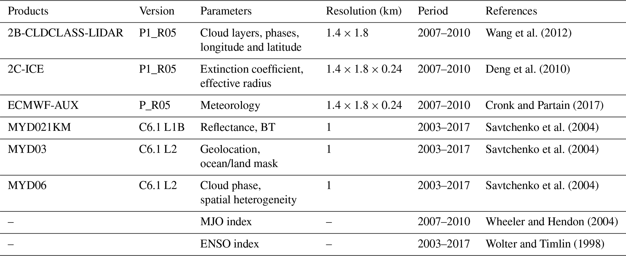
CloudSat, CALIPSO, and Aqua were operated together in the A-Train satellite constellation between May 2006 and February 2018. The A-Train is in a sun-synchronous orbit with an Equator-crossing time around 13:30 local time (LT) in the daytime and 01:30 LT at night. The tight formation of these satellites allows the radar, lidar, and MODIS to observe nearly the same point on Earth within 1 min (Stephens et al., 2018), and thus a straightforward match between these instruments can be performed. The information about all data used in this study is summarized in Table 1. The SEA region is delineated with latitudes between 10∘ S and 30∘ N and longitudes between 80–150∘ E.
2.1 The combined CloudSat–CALIPSO data
Launched in June 2006, the CloudSat satellite carries a cloud profiling radar operated at 94 GHz with a minimum sensitivity of −28 dBZ (Stephens et al., 2002, 2008). The radar's vertical resolution is 480 m but resampled to 240 m, while its horizontal resolution is 1.8 km along track by 1.4 km cross track. The radar is able to penetrate thick clouds but misses optically thin clouds and shallow clouds lower than 1 km altitude (Stephens et al., 2008). The lidar on board CALIPSO launched in April 2006 has vertical and horizontal resolutions of 30 and 333 m in the lower troposphere (i.e., below 8.2 km) and 60 m and 1 km in the upper troposphere (i.e., above 8.2 km) (Winker et al., 2003). The lidar operates at 532 and 1064 nm and is suitable to detect optically thin clouds and aerosols, but its signal is easily attenuated, which limits its ability to penetrate optically thick clouds and to detect anything below. Nevertheless, the lidar has distinct advantages in detecting liquid clouds because (1) the backscattering (βc) from water droplets is much less depolarized than that from ice particles and (2) water layers produce strong lidar returns that attenuate rapidly with altitude at cloud top (Hu et al., 2009; Wang and Sassen, 2001). In cases where thin clouds at any altitudes or shallow clouds near Earth's surface are missed by CloudSat, the CALIPSO lidar can detect these clouds if the lidar attenuation above these clouds is sufficiently small.
To utilize the complementary features of the CloudSat radar and the CALIPSO lidar, the CloudSat Data Processing Center provides a combined radar and lidar cloud classification product called 2B-CLDCLASS-LIDAR (Wang, 2019). This product reports the lidar cloud fraction that records how many lidar profiles are contained in a radar resolution. The cloud top and base heights are also reported for up to five layers in the CloudSat pixels. The cloud layer here extends from cloud top to its base, and the vertical space between two layers is more than 500 m (Sassen and Wang, 2008). Each cloud layer is assigned one thermodynamic phase, either liquid, ice, or mixed. The 2B-CLDCLASS-LIDAR algorithm utilizes cloud top and base temperatures from reanalysis as a first cut for cloud phase determination. If cloud base temperature is lower than −38.5 ∘C, this cloud layer is regarded as ice phase. Liquid phase is determined if cloud top and base temperatures are greater than 1 and −4 ∘C, respectively. While in the temperature range (−40 to 0 ∘C) where supercooled and mixed clouds would exist, potential liquid layers are first located using the feature of strong vertical gradient in lidar signals near liquid tops. If a liquid layer is detected by the lidar, the radar reflectivity factor (Ze) is further adopted to discriminate supercooled liquid from mixed cloud because Ze in mixed cloud is primarily contributed by ice particles. Temperature-dependent Ze thresholds were generated to judge whether ice particles occur in the cloud layer with lidar-detected liquid phase (Fig. 2 in Zhang et al., 2010). When the maximum Ze of the cloud layer is greater than the given threshold, the layer will be classified as mixed cloud; otherwise, it is classified as liquid cloud. When the lidar signal is totally attenuated, the cloud phase is determined only by Ze and temperature, which lowers the confidence level. Also, in cases of thick ice clouds attenuating lidar signals over shallow liquid clouds that are missed by the radar, only ice clouds are reported in the profiles. Biases due to instrument limitations are kept in mind in our analysis.
Despite these limitations, the combined radar–lidar measurements provide comprehensive cloud phase and overlap information. Four years of 2B-CLDCLASS-LIDAR data, version P1_R05 (2007–2010), with lidar cloud fraction greater than zero are used in order to include small-sized clouds.
The CloudSat Level 2C ice cloud property product (2C-ICE) is also used. This product provides ice cloud optical (extinction coefficient in the visible) and microphysical (IWC and Re) properties retrieved from combined CC measurements (Deng et al., 2010). The 2C-ICE algorithm first identifies ice clouds based on the cloud layer and phase from 2B-CLDCLASS-LIDAR. The vertical profiles of Re and IWC are retrieved based on an optimal estimation framework that minimizes a cost function linking the observed and estimated lidar backscatter and Ze via Gauss–Newton iteration. To retrieve ice cloud properties, a modified gamma particle size distribution is adopted. To estimate lidar backscatter and Ze, parameterization of ice habits from Yang et al. (2000) is employed. The 2C-ICE product was evaluated in Deng et al. (2013) by comparing ice cloud properties to field campaign measurements. It was found that the flight-measured-to-2C-ICE-retrieved Re ratio is about 1.05, and the extinction coefficient ratio is about 1.03, hence suggesting excellent consistency between 2C-ICE retrievals with in situ observations. In this study, we integrate the retrieved extinction coefficient profile over depth of the ice layer to obtain ice cloud optical depth (τ). 2C-ICE data (R05) from 2007 to 2010 are used.
Meteorological data are also adopted to interpret the environment for different cloud phases. Temperature, wind, and moisture are from CloudSat's European Center for Medium-Range Weather Forecasts auxiliary product (ECMWF-AUX, 2007–2010), which interpolates the ECMWF variables to each CloudSat profile (Cronk and Partain, 2017).
2.2 CC profile classification
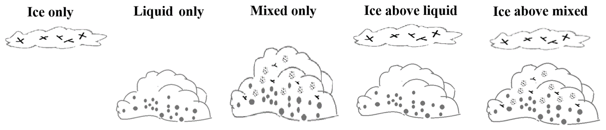
The CC profiles that contain clouds are classified into five groups (Fig. 1), according to the cloud layer and thermodynamic phase information from the 2B-CLDCLASS-LIDAR product. The first group is ice-only cloud, which refers to only ice phase identified in the profile. When ice layers occur above liquid layers, we classify the profile as ice-above-liquid cloud. Similarly, mixed-only, liquid-only, and ice-above-mixed clouds are classified. We do not focus on liquid-above-ice, mixed-above-ice, mixed-above-liquid, or liquid-above-mixed clouds, collectively referred to as “other clouds”, due to their low frequencies (∼0.74 %) over SEA. Note that one cloud phase in each cloud category may contain multiple layers of the same phase. For example, for ice-above-liquid group, there could be more than one ice or liquid layer. While we quantify the frequencies of same-phase overlaps in Sect. 3.1.3, the majority of our analysis groups them into one of the classes listed above to simplify the number of classifications to work with. We lose some intricate cloud vertical structures but still capture the main features of cloud phase overlap.
2.3 The Aqua MODIS data
The Aqua satellite, launched in May 2002, carries MODIS. MODIS has 36 discrete spectral bands, ranging from 0.415 to 14.235 µm, with spatial resolutions varying between 250 m to 1 km (Barnes et al., 1998; King et al., 1992; Platnick et al., 2003). To allow collocating of CC and MODIS pixels, the MYD03 product, which includes longitude, latitude, solar zenith angle, and land/sea mask, is used to obtain MODIS geolocation information. The nearest MODIS 1 km resolution pixels are assigned to the CC data from 2007 to 2010. The distance of the collocated CC–MODIS pixels is usually smaller than 700 m, allowing them to observe nearly the same cloud less than a minute apart. Uncertainties due to collocation are kept in mind during the analysis.
To investigate the spectral signatures of different cloud phases, the MODIS Collection 6.1 Level 1B calibrated radiance data (MYD021KM) are used. The bands selected in this research have center wavelengths at 0.645, 1.375, 1.64, 2.13, 8.55, and 11.03 µm. Ice crystals are more absorptive at the shortwave infrared (SWIR) (e.g., 1.64, 2.13 µm) than liquid droplets, and thus ice clouds have smaller reflectance (R) at the TOA whereas ice and liquid clouds are about equal in reflectance in the visible (0.645 µm) for the same cloud optical depth and particle size – this forms the basis for cloud optical and microphysical retrievals and cloud phase classification for MODIS (Marchant et al., 2016). R1.375 depends on cloud optical thickness and the amount of water vapor above the cloud, since 1.375 µm lies at the center of a strong water vapor absorption band. If cloud top is at a low altitude, the solar photons at 1.375 µm will be largely absorbed by water vapor above cloud, leading to near-zero R1.375 (Marchant et al., 2016). In the IR, we convert the radiances of 8.55 and 11.03 µm to brightness temperature (BT). BT8.5, BT11, and the difference between BT8.5 and BT11 (BTD) are sensitive to cloud top temperature, thickness, and phase (Baum et al., 2012).
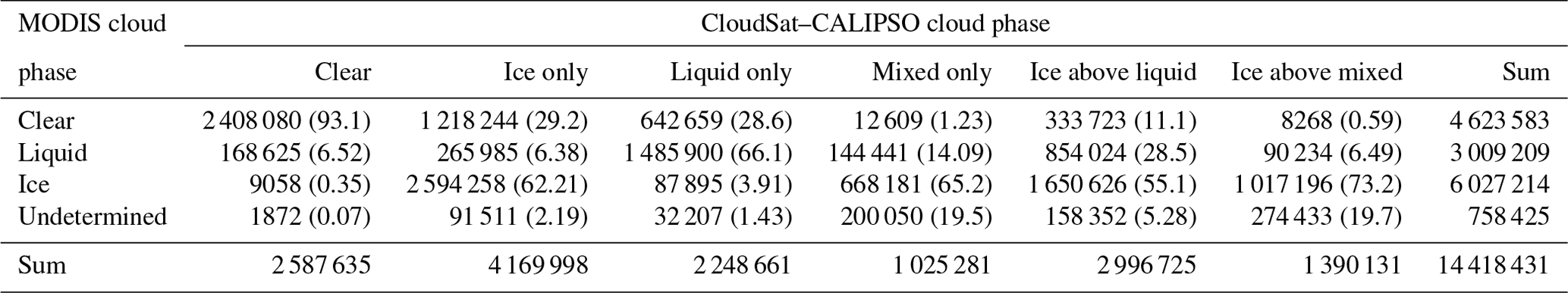
The MODIS Level 2 cloud product (MYD06) provides cloud phase information identified according to three different IR channel pairs, i.e., 8.5 and 11, 11 and 12, and 7.3 and 11 µm, known as the IR-only algorithm (Baum et al., 2012). The product contains three cloud phases: ice, water, and undetermined. Cho et al. (2009) evaluated Collection 5 MODIS IR-only cloud phase using CALIPSO observations. They found that agreements of MODIS to the CALIPSO top layers are 64 % and 34.7 %, respectively, for CALIPSO-detected liquid and ice clouds over the globe. We revisited the comparisons of the latest version of MODIS IR-only cloud (C6.1) to the CC cloud phase (Fig. 1) over SEA in a similar way as Cho et al. (2009). About 66 % CC liquid-only clouds agree with MODIS liquid clouds, which is similar to the global results of Cho et al. (2009). About 62 % of CC ice-only clouds are reported to be ice by MODIS over SEA, agreeing better than the global results of Cho et al. (2009). In addition, most of CC ice-above-liquid (55 %), ice-above-mixed (73 %), and mixed-only clouds (65 %) are reported to be ice phase by MODIS. We also found that 29 % of CC ice-only clouds are reported as clear sky by MODIS, indicating that MODIS misses some thin cirrus in the SEA region – a point also made in Reid et al. (2013). More details about the CC and MODIS cloud phase comparison is displayed in Table 2. In this study, MODIS cloud phase is also adopted to obtain additional cloud phase properties over a wider swath (2330 km) and longer time period than the CC data.
Table 2Comparison of MODIS and CC cloud phase. Number in parentheses represents the percentage (%) of CC phase reported as MODIS cloud phase.
The spatial heterogeneity index (Hσ) defined as the standard deviation over the mean of measured radiances of sixteen 250 m pixels within a 1 km pixel (Liang et al., 2009) is also included in the MYD06 product. The heterogeneity index Hσ usually increases with subpixel-level inhomogeneity and correlates with radiation and remote sensing biases rooted in the plane-parallel assumption (Cho et al., 2015; Fu et al., 2019). The Hσ is reported at 0.645 and 0.865 µm. Here, we adopt Hσ at 0.645 µm because Hσ for 0.865 µm is reported to be zero for saturated pixels, which occurs for thick clouds under certain sun-view geometries encountered in the MODIS data.
The matched Hσ values and MODIS radiances are assigned to cloud phase from 2B-CLDCLASS-LIDAR to investigate cloud spatial heterogeneity and spectral radiation features. Longer MODIS data (2003–2017) are used for analysis of interannual variations in cloud phase. Considering that no visible and SWIR radiances are available at night, only daytime data are considered.
2.4 Meteorological indices
The MJO (Madden and Julian, 1971) consists of large-scale coupled atmospheric circulation and deep convection in the tropical atmosphere. It forms in the Indian Ocean and propagates eastward at a speed around 5 m s−1 across the Maritime Continent and into the equatorial western/central Pacific ocean with an intraseasonal variability of 30–90 d (Zhang, 2005). To understand cloud phase evolution with the MJO, we adopt the Real-time Multivariate MJO (RMM) index (Wheeler and Hendon, 2004), which defines eight MJO phases using two leading empirical orthogonal functions (EOFs) of combined 850 and 200 hPa zonal wind from National Centers for Environmental Predication (NCEP) reanalysis and satellite-observed outgoing longwave radiation (OLR) over the tropical belt. We only focus on strong MJO events with amplitude greater than one.
ENSO has a interannual variability of 3–5 years, and the multivariate ENSO index (MEI) is well suited to identify ENSO events (Wolter and Timlin, 1993, 1998). The new version of MEI is created by the EOF analysis of five variables including sea level pressure, sea surface temperature, surface zonal and meridional winds, and OLR.
3.1 Seasonal variations
3.1.1 Meteorological conditions
To better understand the linkages between cloud properties and large-scale dynamics, meteorological fields are presented in Fig. 2. It shows temperature, specific humidity, wind field, and static stability at the lower (∼850 hPa) and upper (∼180 hPa) troposphere over SEA in four seasons: boreal spring (March, April, and May – MAM), summer (June, July, and August – JJA), autumn (September, October, and November – SON), and winter (December, January, and February – DJF). In the lower troposphere, relatively high and homogeneous temperatures are observed all year round (∼290 K), corresponding to the Indo-Pacific Warm Pool. However, temperatures drop in boreal winter (<285 K; Fig. 2a4) and raise in summer (>290 K; Fig. 2a2) over southeastern China and the South China Sea. In the upper troposphere, temperatures are relatively low at latitudes between 10∘ S–10∘ N (<213 K), while temperatures over South Asia in summer are 1–3 K higher than in other seasons. Similarly, high humidity (>10 g kg−1 at lower troposphere and >0.03 g kg−1 at upper troposphere) is located south of 10∘ N latitude during spring and winter (Fig. 2b1, b4), while in autumn (Fig. 2b3), the humidity pattern is quite symmetric about the Equator. Also, air is especially moist over South Asia during summer than in other seasons at both the lower and upper troposphere. The summer high temperature and humidity over South Asia are related to the heating and convection over the Tibetan Plateau, which maintains a hot and humid upper troposphere, and the South Asian anticyclone (Yeh, 1982). The summer monsoon also helps transfer a large amount of moisture from the Indian Ocean to Asia (Fig. 2c2).
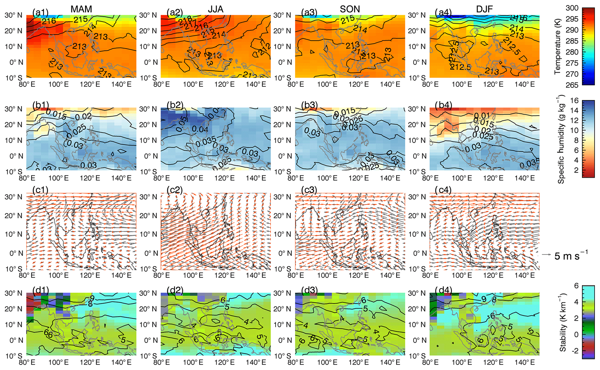
Figure 2(a1–a4) Temperature, (b1–b4) specific humidity, (c1–c4) wind field, and (d1–d4) static stability derived from the ECMWF-AUX data; shade for 850 hPa, contour for 180 hPa, grey vectors for wind field at 850 hPa, and red vectors for 180 hPa.
The seasonality of the wind field is evident (Fig. 2c1–c4). In the lower troposphere, the southwesterly wind flow brings warm and humid air to South Asia in summer when the ITCZ is located north of Equator, providing favorable conditions to form clouds and precipitation (summer monsoon). The wind direction in the upper troposphere is northeasterly, which is nearly opposite to that at the lower troposphere. In DJF, the ITCZ shifts to the Southern Hemisphere, and the wind flow reverses. The prevailing northeasterly flow near the lower troposphere (winter monsoon) is also opposite to the wind direction at the upper troposphere (southwesterly). However, the upper troposphere wind is much weaker in winter than in summer because the summer South Asian anticyclone above the Tibetan Plateau enhances the upper troposphere wind flow (Yeh, 1982). The spring and autumn are two transition seasons of summer and winter monsoonal flows.
The lower-troposphere static stability, LTSS = , and the upper-troposphere static stability, UTSS = , are shown in Fig. 2d1–d4, where the θ is potential temperature in units of kelvin. The tropopause height is defined following the World Meteorological Organization; i.e., the lowest level where lapse rate is 2 ∘C km−1 or less, and the average lapse rate between this level and all higher levels within 2 km is smaller than 2 ∘C km−1 (Grise et al., 2010). Figure 2d1–d4 reveal that LTSS is usually smaller over land than over ocean. Small LTSS values (<4 K km−1, yellow-green color) over ocean correspond to a wetter atmosphere (Fig. 2b). Relatively larger LTSS (>4 K km−1) occurs in winter and spring such as over the East and South China seas. The LTSS has been proven to be an important parameter indicating low-level cloud formations. For instance, Klein and Hartmann (1993) showed that 1 ∘C increase in stability is associated with a 6 % increase in stratus cloud area coverage. The spatial pattern of UTSS is similar to that of LTSS.
3.1.2 Occurrence of all clouds
This sections focuses on cloud spatial distributions over SEA. The horizontal occurrence frequency, defined as the ratio of total cloudy number to the total observation sample in each 5∘ long × 2∘ lat grid derived from the 2B-CLDCLASS-LIDAR data, is shown in the upper panels of Fig. 3. The zonal latitude–altitude cross sections, obtained by cloudy number in each 2∘ lat × 250 m height cell divided by the observation sample in that cell, are displayed in the lower panels of Fig. 3.
Over SEA, the annual mean cloud frequency is about 81.4 %, being smaller in winter and larger in summer (Table 3). As expected, seasonal variations in cloud occurrence are generally associated with the movement of large humidity, warm temperature, and low stability in the lower and upper troposphere (Figs. 2, 3). Clouds frequently occur in Southeast Asia during the summer monsoon season, while their frequency shifts to the Malaysia and Indonesia regions as the summer monsoon retreats and the ITCZ shifts southward. The cross sections (Fig. 3b1–b4) display prevailing high-level clouds located at around 10–15 km, matching to the ubiquitous nature of cirrus over the warm pool regions (Sassen et al., 2008). These ice clouds have their largest frequencies centered ∼12∘ N in summer but shift to south of the Equator in winter, i.e., moving with the ITCZ and the monsoon.
While it is clear that clouds favor warm, humid, and unstable conditions, large cloud occurrences are found in other conditions in the region. Frequent cloud occurrence (∼70 %) is also observed over southeastern China and the East China Sea during winter when the atmosphere is cold, dry, and stable (Figs. 2, 3a4). These winter clouds north of 10∘ N usually have low cloud heights (<5 km) with little cirrus above as seen from the cross section (Fig. 3b4).

Figure 3Cloud occurrence frequency derived from 2B-CLDCLASS-LIDAR, for (a1–a4) horizonal distribution and for (b1–b4) zonal latitude–altitude cross section.
While Fig. 3b displays a vertical cross section of cloud occurrence frequencies, it says little about cloud overlap frequencies. As shown in Yuan and Oreopoulos (2013), low-level clouds have a high chance of being overlapped by upper clouds in the warm pool region. In the next section, we will examine cloud overlap with a focus on cloud phase.
3.1.3 Occurrence of cloud phase
As stated in Sect. 2.2, we classify clouds according to cloud phase and cloud layer in five main groups: ice-only, liquid-only, mixed-only, ice-above-liquid, and ice-above-mixed clouds. Each group contains both single and multiple layers of the same phase. Our analysis (Table 3) shows that one-layer–one-phase clouds have much larger frequency than multilayer same-phase clouds. For example, multilayer ice-only clouds (∼8.6 %) occur less frequently than one-layer–ice-only clouds (20 %). Liquid-only clouds mostly form in a single layer (14 %), and the frequency of multilayer liquid-only clouds is only 2 %. A careful comparison between single and multiple layers of the same-phase clouds shows no significant difference in the properties that we are interpreting, which justifies our simpler classification.
Figure 4 shows horizontal and vertical distributions of the five cloud groups as defined in Fig. 1. The mean occurrence frequency of each cloud class in four seasons over ocean and land is summarized in Table 3. The five cloud groups display visible differences in both of their mean frequencies and spatial distributions. Ice-only clouds (Fig. 4a) occur most frequently (∼28.6 %) among all cloud classes. These clouds widely spread in the tropical belt and prefer the locations north of the Equator in summer but move to the south in winter. Ice-only clouds mainly are located at high altitudes between 10 and 15 km (Fig. 4b), corresponding to the prevalent tropical cirrus discussed in many other studies (Hong and Liu, 2015; Reid et al., 2013; Sassen et al., 2008).

Figure 4Occurrence frequency of the five cloud groups derived from 2B-CLDCLASS-LIDAR; (a) for horizonal distribution and (b) for zonal latitude–altitude cross section.
Table 3Cloud occurrence frequency (%) derived from 2B-CLDCLASS-LIDAR. In the section ocean vs. land, the number outside parentheses represents both land and ocean. The first number in parentheses is for ocean, and the second one is for land. In the section single vs. multiple cloud layers, the first number in parentheses represents single layer, and the second number is for multiple layer.
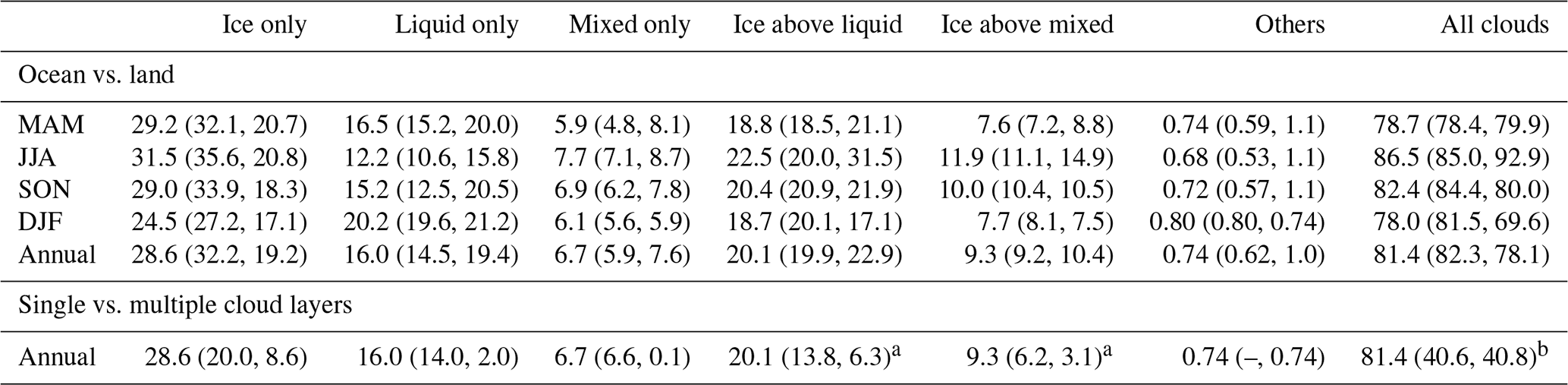
a The single and multiple layers represent the overlying ice clouds only. b All single-layer clouds are the summation of single-layer–ice-only (20.0 %), liquid-only (14.0 %), and mixed-only (6.6 %) clouds, while all multilayer clouds include multilayer ice-only (8.6 %), liquid-only (2.0 %), mixed-only (0.1 %), ice-above-liquid (20.1 %), ice-above-mixed (9.3 %), and other (0.74 %) clouds.
In contrast, liquid-only clouds (Fig. 4a) are widely distributed over southeastern China and the East China Sea and show large seasonality. These liquid-only clouds mostly have their cloud tops lower than 3 km (Fig. 4b). They are the so called “Chinese stratus” by Klein and Hartmann (1993) associated with lower-troposphere cold and dry air and large LTSS (Fig. 2). Elsewhere, liquid-only clouds have very small frequencies (<10 %). The annual mean frequency of liquid-only clouds is ∼16.0 %.
Ice-above-liquid clouds have an annual mean occurrence frequency of ∼20.1 % (Fig. 4a). Ice layers located at 10–15 km cover the underlying liquid clouds mostly with heights below 3 km (Fig. 4b). These clouds occur frequently over southern China and Southeast Asia during the summer monsoon season and move to western Pacific Ocean and Malaysia–Indonesia regions in winter.
The areas where widely distributed ice-only and ice-above-liquid clouds are also associated with relatively frequent mixed-only (annual frequency ∼6.7 %) and ice-above-mixed clouds (annual frequency ∼9.3 %) (Table 3) such as in Southeast Asia in summer and the Malaysia–Indonesia region in winter. Mixed-only clouds are mature convective clouds as seen from their cross sections (Fig. 4b), which extend from near surface up to above 15 km. Nevertheless, near 30∘ N from fall through spring where liquid-only clouds dominate, there exist relatively frequent mixed-only clouds with their top below 10 km. The ice-above-mixed clouds, frequently occurring at 6 km, are more likely under development with mixed-layer tops reaching to around 10 km. If the mixed layers develop higher, they would merge with the overlying ice clouds and are classified into the mixed-only cloud class. Overall, liquid-only clouds are associated with high LTSS and lower temperature in the lower troposphere, agreeing with the relationship of low-level clouds with stability (Klein and Hartmann, 1993; Li et al., 2014). In contrast, ice-only, ice-above-liquid, ice-above-mixed, and mixed-only clouds, collectively named as “ice-contained clouds”, favor a humid, warm, and unstable environment.
Figure 5 further summarizes the mean and standard deviation of the meteorological variables discussed in Fig. 2 from the ECMWF-AUX product for the five cloud groups in summer and winter seasons over ocean (to avoid the low static stability over land). In the lower troposphere, all cloud groups in summer tend to have smaller LTSS and higher temperature and humidity than in winter (Fig. 5a, b). The standard deviations in summer are also smaller, being consistent with a more homogeneous spatial pattern of the meteorological fields (Fig. 2). In winter the liquid-only clouds tend to have a much smaller humidity and colder temperature corresponding to the occurrence of the Chinese stratus (Klein and Hartmann, 1993). For those ice-contained clouds, they are still located in a relatively warm, moist, and unstable atmosphere, but their standard deviations are much larger than that in summer, agreeing with the less homogeneous spatial pattern of meteorology in winter (Fig. 2).
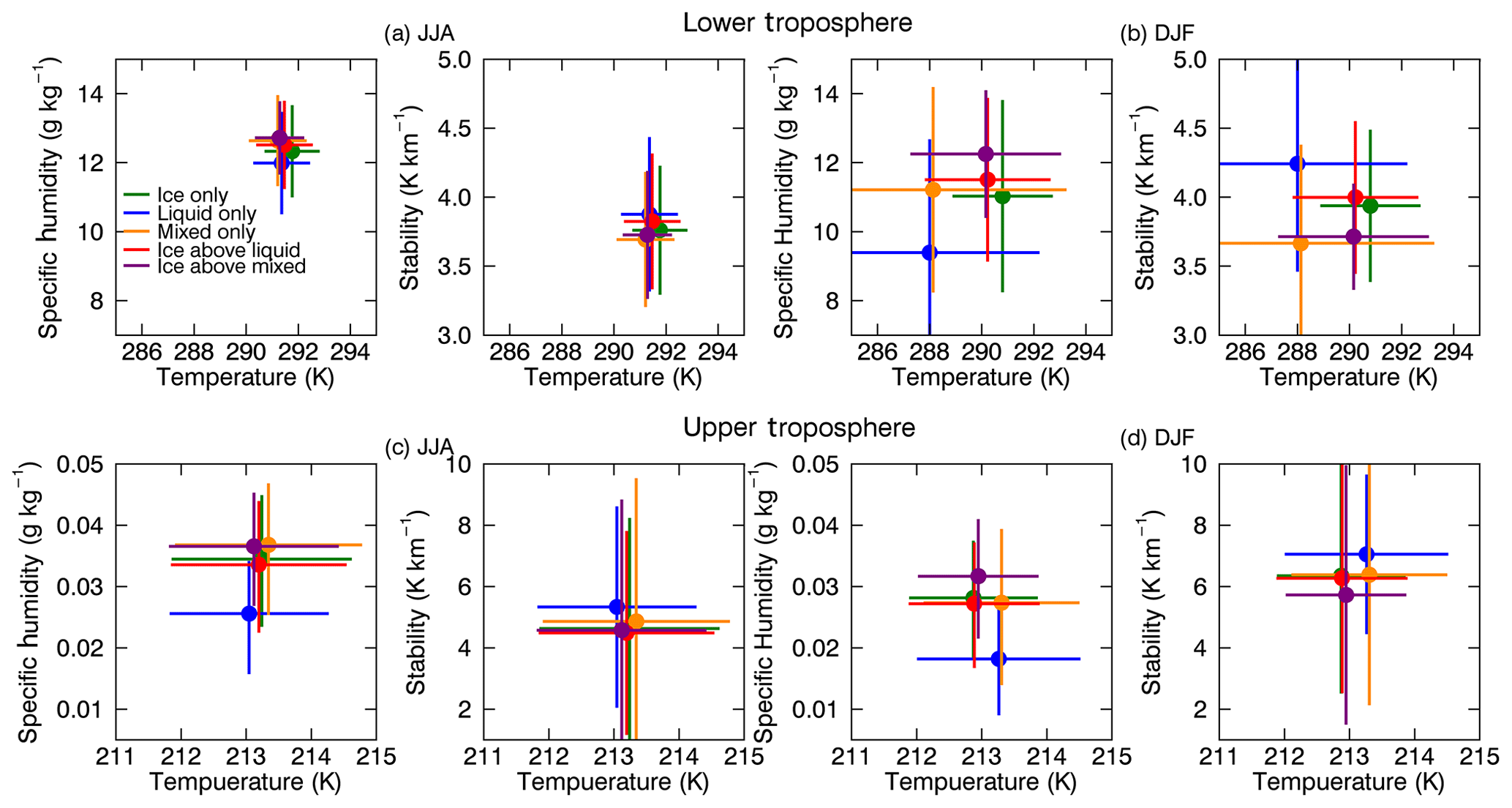
Figure 5Mean and standard deviation of meteorological variables over ocean for the five cloud groups.
In the upper troposphere (Fig. 5c, d), the relationship between the five cloud types and meteorology is similar in both summer and winter, with liquid-only clouds deviating from ice-contained clouds. The ice-contained clouds relate to smaller UTSS as reported in Li et al. (2014). Also, ice-only and ice-above-liquid clouds share very similar upper tropospheric meteorology as their mean and standard deviations are nearly the same, which is not surprising because the low stability and high moisture are essential to maintain cirrus (Christensen et al., 2013; Li et al., 2014). However, the specific humidity in the upper troposphere of ice-above-mixed clouds is larger than both ice-only and ice-above-liquid clouds (Fig. 5c, d), which may reveal that convection below brings moisture to the upper troposphere.
3.1.4 Distributions of cloud phase properties
Figure 6 presents the probability distribution function (PDF) of cloud properties including cloud top for all cloud phases and base, geometric thickness, τ, and Re for ice layers from the 2C-ICE product. The averages of the cloud properties in the four seasons are summarized in Table 4.

Figure 6Annual PDFs of (a) cloud top, (b) base, (c) geometric thickness, (d) optical depth, and (e) effective radius for ice clouds including both ocean and land. The vertical dashed lines in (a)–(e) indicate the median values of the PDFs; (f) cloud top for liquid-only cloud and the liquid below ice and (g) cloud top for mixed-only and the mixed cloud below ice. In (f) and (g), solid and dashed curves are for ocean and land, respectively. Cloud top and base bins adopt an interval of 0.5 km. Ice τ and Re bins use an interval of 0.1 on a log scale and 1 µm, respectively.
Table 4Average of cloud properties for the five cloud groups over ocean and land.

a T for cloud top. b B for cloud base. c G for geometric thickness. Subscripts: i for ice, w for water, and m for mixed.
The properties of ice layers in the three categories – ice-only, ice-above-liquid, and ice-above-mixed clouds – are displayed in Fig. 6a–e. We combine both land and ocean data to investigate the distributions of ice layer properties, because their PDFs display similar shapes between that over land and ocean (figure not shown); however, their averages are separately summarized in Table 4. The three categories of ice layers share many similarities in their PDFs: the modes of ice top PDFs (∼16 km) and base (∼12.5 km) slightly greater than their means and medians (Table 4 and vertical dashed lines in Fig. 6). The modes of geometrical thickness PDFs are around 1 km, which are smaller than their mean and median values of 2–4 km (Fig. 6c and Table 4). These statistics demonstrate that the distributions of ice clouds skew to higher locations and thinner thickness, corresponding well to the properties of cirrus near the tropopause (Haladay and Stephens, 2009; McFarquhar et al., 2000). In addition, the τ PDFs show two modes for the three types of ice layers and the Re PDFs with their modes slightly greater than 15 µm.
There also exist differences between the three groups of ice layers. For example, ice-only clouds tend to locate 0.4–1.4 km lower over land than ocean, and the lower location may allow more moisture to feed into ice clouds, which may explain why ice clouds over land have mean τ values of 0.6–1.6 and Re of 3–5 µm larger than those over ocean (Table 4). Compared to ice-only clouds, the ice layers above liquid or mixed clouds show much less land–ocean contrast in these properties (Table 4). Also, the ice layers above liquid clouds contain about 73.8 % of samples with geometrical thickness <3.0 km and about 91.5 % of samples with ice τ<3.0 – the threshold often used to define cirrus (Sassen et al., 2008) (Fig. 6c, d). In contrast, ice-only clouds are thicker with larger means, medians, and Re (Table 4), which are contributed by more ice-only cloud samples with geometrical thickness >3.5 km, τ>1.6, and Re>60 µm (Fig. 6). Due to the fact that lidar signals are attenuated when cloud τ>3.0 and the radar fails in detecting shallow clouds, some ice-above-liquid clouds (e.g., thick ice over shallow liquid) could be classified into the ice-only group, leading to some sampling biases to the mean ice τ and Re. However, in the ice τ range of 1.6–3.0 where CALIPSO can penetrate the cloud, ice-only clouds have a total frequency of ∼0.11 in this τ range, being higher than the frequency (∼0.07) of the other two groups and demonstrating a higher probability of ice-only clouds being thicker.
For liquid or mixed layers, we only focus on cloud tops, because the determination of cloud base suffers from larger uncertainties than cloud top due to the limitation of instruments; i.e., CloudSat radar has difficulty in distinguishing the cloud base near Earth's surface, and the CALIPSO lidar signal is attenuated by clouds with optical thickness greater than 3 (Hu et al., 2009; Stephens et al., 2008). For the liquid top PDFs (Fig. 6f), there are two modes for the liquid below ice clouds (green). One mode is located at 1 km for ocean (2–3 km for land), and the other is located at ∼6 km for both ocean and land. We further obtain the spatial distributions of the liquid below ice clouds with a liquid top greater than and lower than 5 km (figure not shown). It is shown that liquid clouds with a top <5 km are widely distributed over SEA, while those with a liquid top >5 km are more concentrated in locations with a latitude <10∘, corresponding to a more unstable environment as shown in Fig. 2. In another words, greater moisture and small LTSS allow liquid clouds to develop deeper. For liquid-only clouds, they have a much higher frequency at the PDF mode of 1 km, and the second mode is not evident. The averaged top value of the liquid below ice clouds is higher than liquid-only clouds (Table 4).
For the mixed layers below ice clouds (Fig. 6g), the mode of cloud top PDF (cyan) is at around 6 km, and the mean is about 8.5 km, with the values over ocean about several hundred meters higher than that over land (Table 4). Note that as the mixed layers develop deeper, e.g., top >10 km, and merge with the upper ice layers, these clouds would be grouped as mixed-only clouds. For mixed-only clouds, the primary mode of cloud top PDF is at around 16 km, and the secondary mode is at around 6 km. The primary mode is much higher over ocean than over land, while the secondary mode is higher over land, indicating that more mixed clouds over land are under development around 13:30 local time. This agrees with the results in Nesbitt and Zipser (2003) that convective clouds keep developing in the early afternoon and reaching toward an intensity maximum in the late afternoon over land, while diurnal variation in convection intensity is insignificant over ocean.
3.1.5 Spatial heterogeneity of cloud phase
Section 3.1.1–3.1.4 discussed the macrophysical properties including spatial distributions, cloud thickness, top and base heights for five cloud groups, and their relationship with meteorology based only on CC data. In this section, by combining the MODIS and 2B-CLDCLASS-LIDAR data, we investigate how the spatial heterogeneity index (Hσ) relates to cloud phase. The Hσ not only is closely related to cloud micro- and macrophysical properties but also affects the accuracy of cloud retrievals from passive sensors and radiative transfer modeling (Ham et al., 2015; Zhang and Platnick, 2011). Only ocean data are considered to avoid complications with the effects of land surface heterogeneity on interpreting results.
The Hσ PDFs for the CC clear sky and the five cloud groups are shown in Fig. 7a. The PDF of CC clear sky has a sharp peak at Hσ∼0.01, indicating that clear sky is usually spatially homogeneous. For cloudy sky, liquid-only clouds are the most heterogeneous among all cloud groups, with Hσ ranging from 0.01 to 1, with a peak of ∼0.5. The ice-only clouds in contrast are homogeneous, as the PDF has a peak close to that of clear sky. This suggests that the biases in retrieved optical and microphysical properties of clouds from passive sensors caused by the plane-parallel assumption will be larger for water clouds compared to ice clouds in the SEA region. Indeed, MODIS liquid Re differences retrieved from three wavelengths (1.6, 2.1, and 3.7 µm) are especially large over this region (up to 10 µm) (Zhang and Platnick, 2011; Fu et al., 2019). Care is therefore recommended when using the MODIS cloud microphysical products in this region, such as in interpreting the cloud–aerosol relationship over SEA (e.g., Ross et al., 2018).
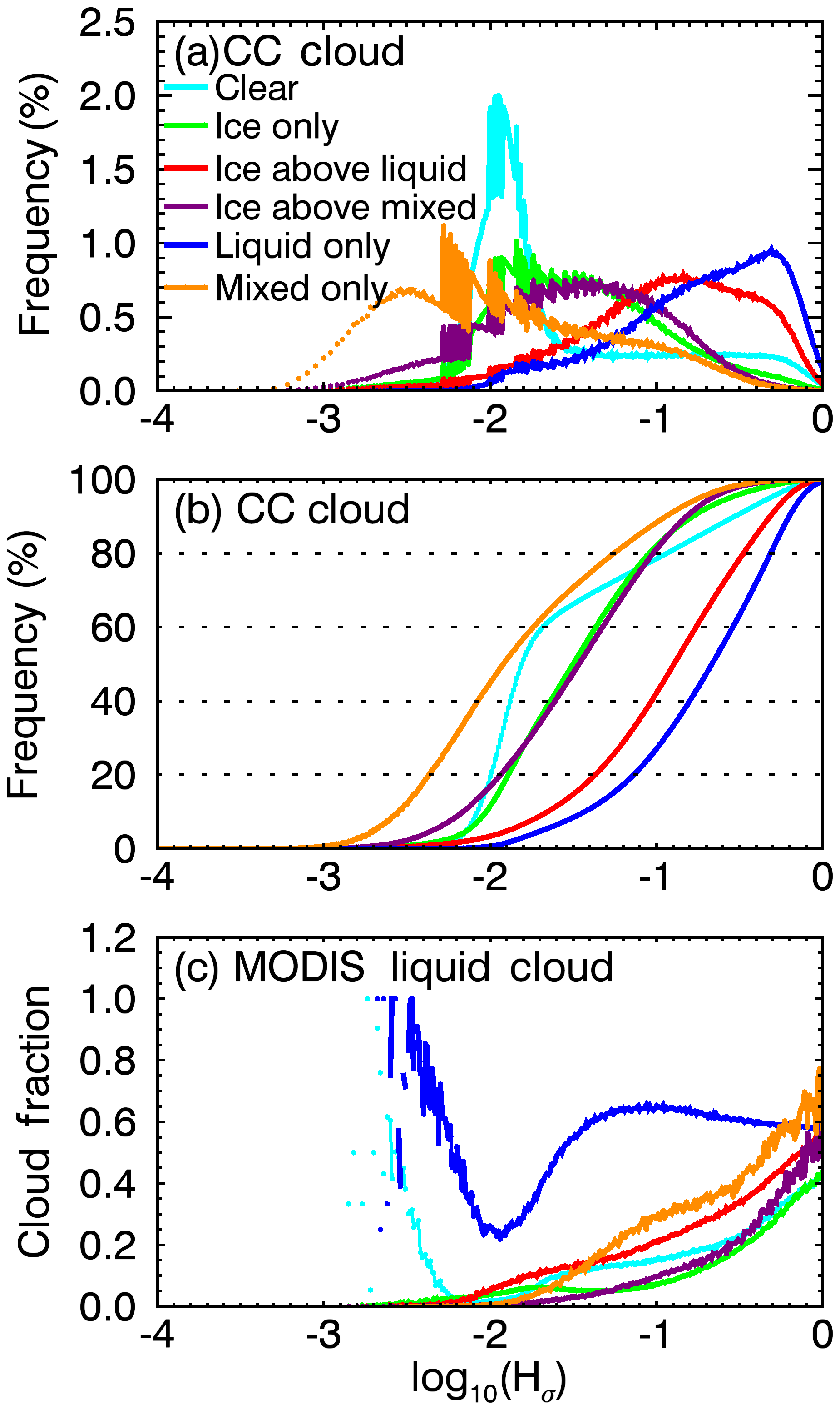
Figure 7(a) Annual PDFs of spatial heterogeneity for CC clear sky and the five cloud groups; panel (b) is the same as (a) but for CDF; (c) liquid cloud fraction in the 5 km × 5 km surrounding of the collocated CC–MODIS pixel derived from the MYD06 IR cloud phase retrievals. Hσ bin interval is 0.01 on a log scale.
For ice-above-liquid clouds, the PDF curve moves slightly to a smaller Hσ region compared to liquid-only clouds, as the overlying ice clouds have a spatial smoothing effect on the radiation emerging from the liquid clouds below. However, due to the small optical thickness of the overlying ice clouds, radiation from underlying liquid clouds dominate (Sect. 3.1.4). The Hσ PDF of ice-above-mixed clouds is similar to that of ice-only clouds but with some samples having Hσ smaller than for clear sky (e.g., Hσ<0.01). This feature is more obvious for the mixed-only clouds, which have about 50 % of their samples with Hσ<0.01 (Fig. 7b), indicating that these clouds are extremely homogeneous. These cases of very smooth ice-above-mixed and mixed-only clouds correspond to high mixed-layer tops and large reflectance at 0.645 µm (discussed in next section), which are associated with deep convection. These clouds are locally homogeneous and hence favor the plane-parallel assumption in radiation computation (Ham et al., 2015).
Note that CC clear sky and ice-only, ice-above-mixed, and mixed-only clouds are usually homogeneous, but there exist some heterogeneous cases. The PDF of clear sky has a long tail of Hσ values extending up to 1 (Fig. 7a) and has about 20 % of samples with Hσ values greater than 0.1 (Fig. 7b). Mismatch of pixels in collocation or difference in spatial resolutions of CC (1.8 km × 1.4 km) and MODIS (1 km) can contribute uncertainties to the Hσ of CC clear sky. Yet, with a focus on the clear-sky pixels on which both CC and MODIS agree, they behave nearly the same as those of CC clear sky, as shown in Fig. 7a, indicating that the long tail is due to the significant amount of misdetection of small subpixel clouds by both MODIS and CC. Indeed, many small liquid clouds with sizes ranging from a few tens to hundreds of meters can go undetected by MODIS (Zhao and Di Girolamo, 2006). We revisit the MODIS and Advanced Spaceborne Thermal Emission and Reflection Radiometer (ASTER) data (15 m resolution) used in Zhao and Di Girolamo (2006) over the tropical western Atlantic. The long tail of the Hσ PDF is significantly reduced, i.e., frequency change from 0.3 % to 0.1 % at Hσ∼0.1, when the ASTER data are applied to exclude the MODIS clear-sky pixels that contain ASTER-reported clouds. This further affirms that the undetected clouds in MODIS and CC clear-sky pixels contribute to large Hσ values, which may at least impact 20 % of clear-sky samples whose Hσ>0.1 (Fig. 7a, b).
To further investigate this last point, we calculate the MODIS liquid cloud fraction, defined as the ratio of liquid cloud samples based on the MYD06 product to the total 25 pixels in a 5 km by 5 km surrounding of the collocated CC–MODIS pixel. As shown in Fig. 7c, as Hσ increases, a larger fraction of MODIS liquid clouds is observed around the CC clear sky and ice-only, mixed-only, and ice-above-mixed clouds. This indicates that the heterogeneous pixels could also be due to undetected liquid clouds in the subpixels.
Figure 8 shows the mean Hσ for CC clear sky, the five cloud groups, and all sky that includes both clear and cloudy sky. As expected, ice-only, ice-above-mixed, and mixed-only clouds are homogeneous everywhere (), with some relatively large values (Hσ∼0.1) in the liquid-only-cloud prevailing regions such as the East China Sea in winter (Figs. 4, 8b4, d4, f4). As liquid-only clouds are the most heterogenous, they show the largest spatial Hσ values over SEA (Fig. 8c1–c4). Also, the Hσ values over the East China Sea in spring, fall, and winter are relatively smaller than the Hσ in other regions, implying that the Chinese stratus that favor dry and stable meteorological conditions are less heterogenous than other liquid-only clouds (Fig. 8c1–c4). Ice-above-liquid clouds (Fig. 8e1–e4) are smoother than liquid-only clouds, and their relatively small values tend to coincide with frequent ice-above-liquid cloud occurrence that are associated with the monsoon and ITCZ, such as in the Malaysia–Indonesia region in winter or the North Indian Ocean in summer (Fig. 4). The Hσ pattern of CC clear sky (Fig. 8a1–a4) shows smaller values than ice-above-liquid clouds but larger values than ice-only, ice-above-mixed, and mixed-only clouds. Also, the places with large Hσ values of CC clear sky are consistent with those with frequent occurrence of ice-above-liquid or liquid-only clouds, which in turn indicates the high chance of undetected liquid clouds increasing the subpixel variability.
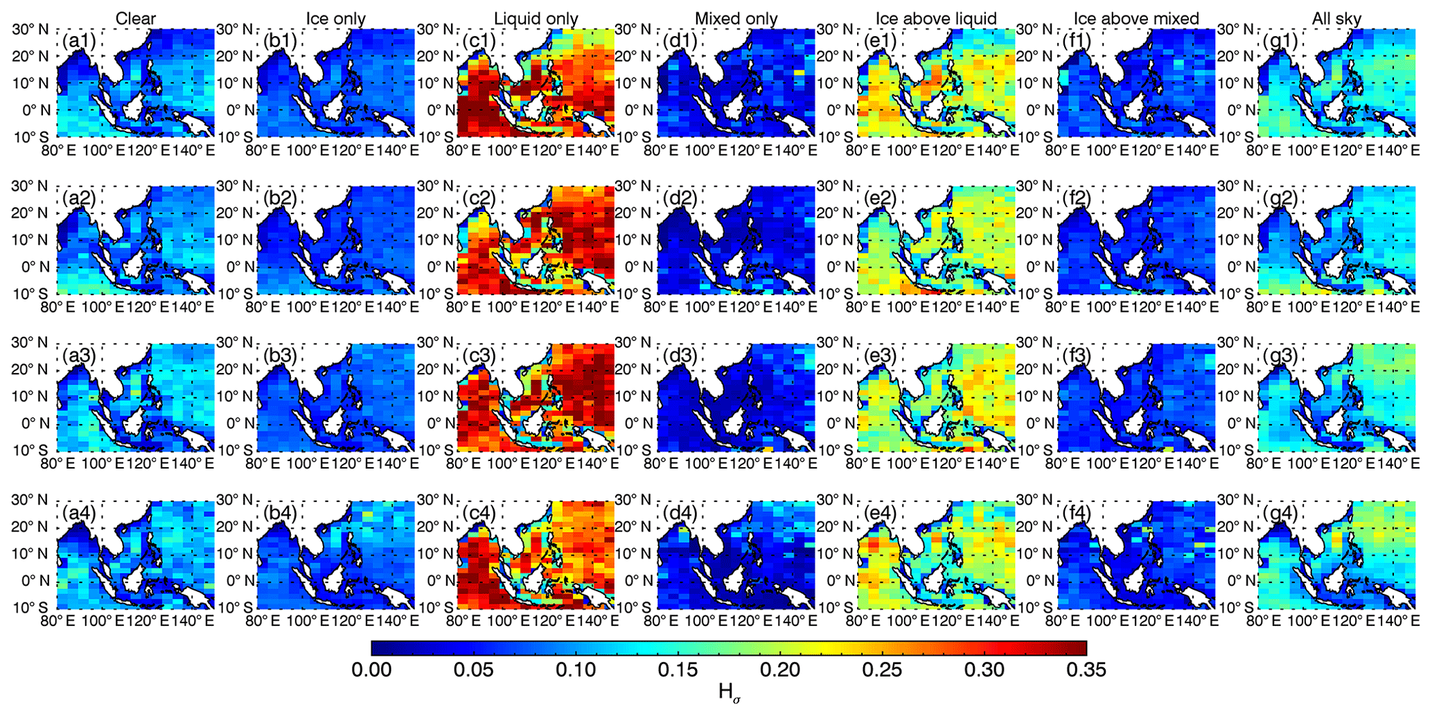
Figure 8Spatial distributions of Hσ for clear sky, the five cloud groups, and all sky from panels (1) to (4) for MAM, JJA, SON, and DJF, respectively.
For all sky (Fig. 8g1–g4), the small Hσ values occur north of the Equator in summer, including the Indian Ocean and South China Sea. The pattern is quite symmetric about the Equator in fall and moves south of the Equator in winter – consistent with the shift of the monsoon and ITCZ. This is because the small Hσ values are primarily contributed by ice-only clouds due to their large occurrence frequency (Fig. 4) and spatial homogeneous features. In contrast, the pattern of large Hσ agrees more with that of liquid-only cloud occurrence (Fig. 4).
Overall, liquid clouds are spatially heterogeneous over SEA, whereas ice-only and mixed clouds are usually homogeneous. Due to the smoothness of the overlying ice clouds, ice-above-liquid clouds are less heterogenous than liquid-only clouds, but their Hσ values are still large because overlying ice clouds are optically thin and the emerging radiance from underlying liquid clouds dominates. Clear sky is smooth with Hσ∼0.01, but undetected liquid clouds increase its subpixel variability. The seasonal variations in all-sky Hσ spatial patterns are in accordance with cloud movements associated with the monsoon and ITCZ.
3.1.6 Spectral radiative feature
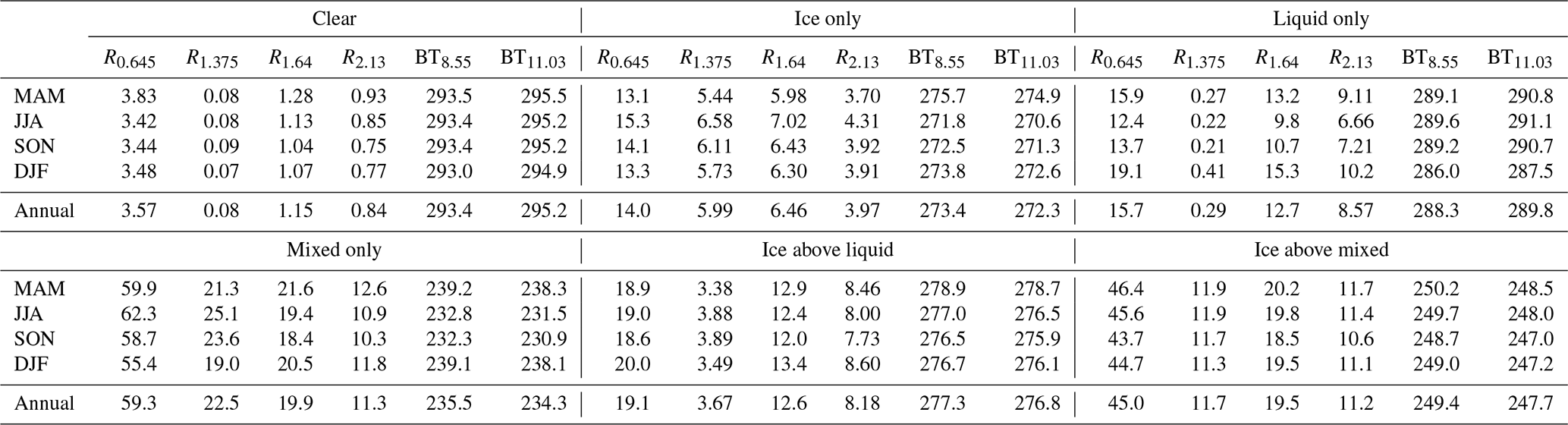
This section examines the spectral radiance at the TOA observed by MODIS for the CC clear sky and the five cloud groups defined in Fig. 1 to investigate how radiative features observed at the TOA relate to cloud phase. Similar to Sect. 3.1.5, only ocean data are adopted. The averages of the reflectance (R) and the brightness temperature (BT) (not weighted by cloud occurrence frequency) for each cloud group are shown over SEA in Fig. 9 and summarized in Table 5, while the PDFs and the cumulative distribution functions (CDFs) are displayed in Fig. 10.
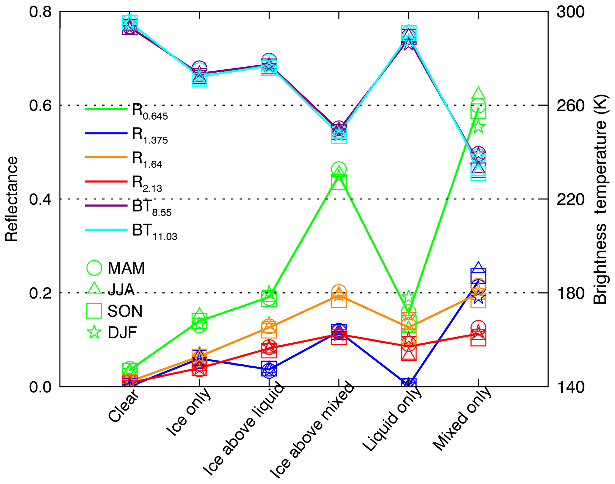
Figure 9Average reflectance and brightness temperatures over ocean for clear sky and the five cloud groups, including all solar zenith angles. The sold lines represent annual mean, and symbols denote seasonal averages.
Table 5Average reflectance at 0.645, 1.375, 1.64 and 2.13 µm (unit: %) and brightness temperature at 8.55 and 11.03 µm (unit: K).
The PDF of R0.645 for clear sky shows a narrow peak at R0.645∼0.02 (Fig. 10a1). Ice-only cloud shows its PDF peaks near the clear-sky peak, and its CDF shows that about 80 % of its samples have R0.645<0.2, proving the thin features of ice-only clouds over SEA and agreeing with their small optical depths in Fig. 6d. Similarly, for liquid-only cloud, the PDF also shows its mode near that of clear sky. A large fraction of liquid-only clouds are optically thin clouds (e.g., more than 75 % of liquid-only clouds with R0.645<0.2), being consistent with the findings of Leahy et al. (2012) that the thin marine low-cloud fraction is greater than 80 % for the SEA region. Ice-above-liquid clouds have a larger mean R0.645 than either ice-only or liquid-only clouds in the column (Table 5 and Fig. 9), but ice-above-liquid clouds still contain more than 60 % of samples with R0.645<0.2, further demonstrating the ubiquity of thin clouds over SEA. Many of these thin clouds often go undetected by MODIS as shown in Table 2, where around 11 % of CC ice-above-liquid cloud and 30 % of CC liquid-only and ice-only cloudy samples are reported to be clear sky by MODIS. The largest average R0.645 is seen in mixed-only clouds (∼0.59), followed by the ice-above-mixed clouds (∼0.45). Their PDFs are broad and flat, but the frequencies at R0.645>0.4 are evident as displayed in Fig. 10a1. Their CDFs reveal that 60 % of ice-above-mixed and 80 % of mixed-only clouds have R0.645>0.4, indicating that these clouds are geometrically deep (consistent with Fig. 4) and optically thick.
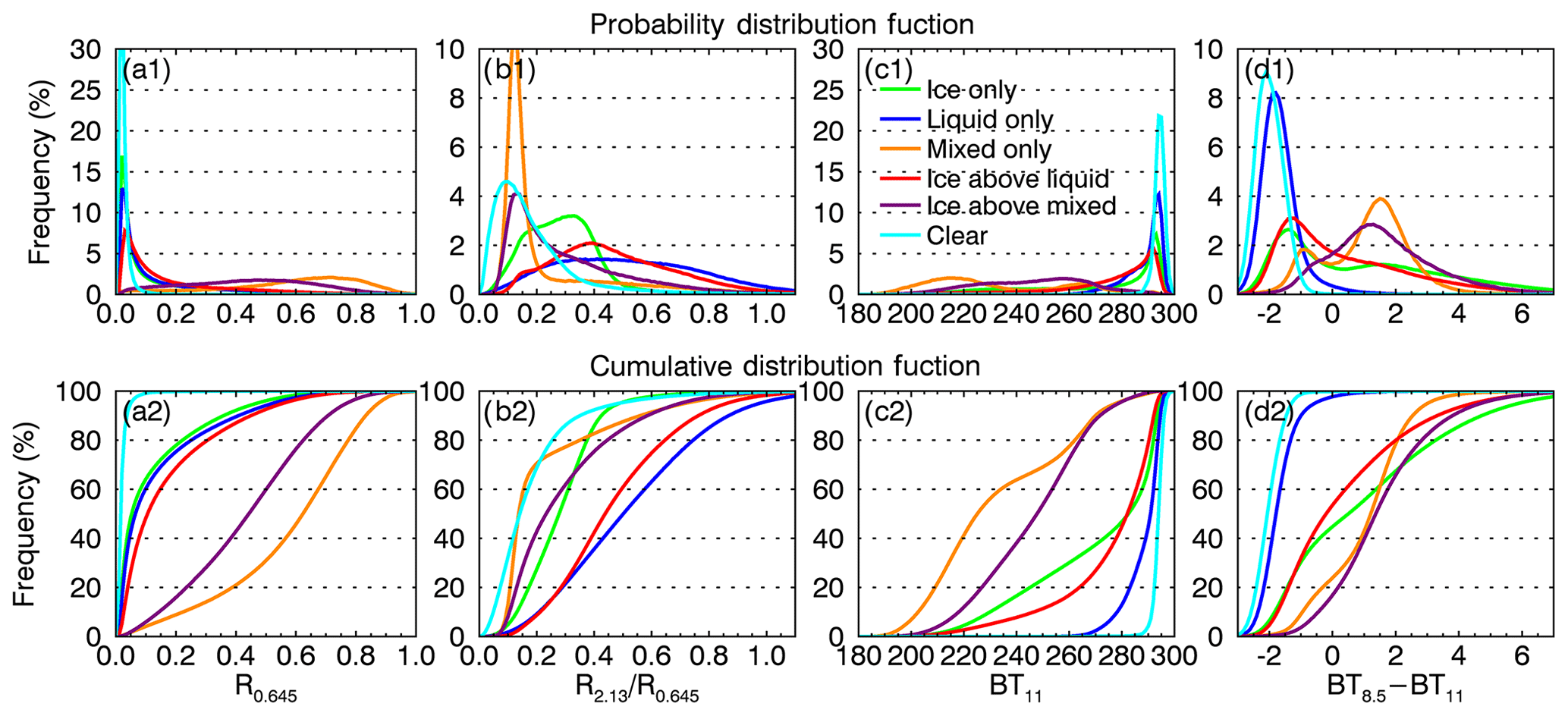
Figure 10The annual PDFs and CDFs of reflectance at 0.645 µm, reflectance ratio, BT at 11 µm, and BTD between 8.5 and 11 µm. The intervals for reflectance, reflectance ratio, BT, and BTD are 0.01, 0.01, 1, and 0.1 K, respectively.
At 1.64 µm, the average R1.64 of ice-above-liquid clouds is nearly same as liquid-only clouds (∼0.13) (Table 5 and Fig. 9). Both these cloud groups are more reflective than ice-only clouds (average R1.64∼0.06). The average R1.64 of ice-above-mixed and mixed-only clouds is about 0.20, implying that ice-above-mixed clouds are optically thick enough to reach the asymptotic reflectance, and mixed-only clouds do not increase R1.64. Similarly, the average R2.13 of both mixed-only and ice-above-mixed clouds is also nearly equal (0.11), which in turn demonstrates their large thickness. The curve of R2.13 across different cloud groups (Fig. 9) shows a similar shape with that of R1.64 but with a smaller magnitude, owing to the larger imaginary part of refractive index of water and ice at 2.13 µm than at 1.64 µm. Particularly, the imaginary part of ice refractive index is larger than water at both wavelengths. Hence, when examining the reflectance ratio of SWIR (1.64 or 2.13 µm) to the visible (0.645 µm), we would expect that liquid-only clouds show a larger ratio than any other cloud groups. Because the Aqua MODIS 1.6 µm band has many dead detectors (King et al., 2013), we display the PDF and CDF for reflectance ratios from 2.13 to 0.645 µm () to further emphasize the spectral features of different cloud phases (Fig. 10b1 and b2). As expected, the PDF of liquid-only cloud extends to large reflectance ratio regions, and the same is true for ice-above-liquid clouds (Fig. 10b1). Moreover, there are about 60 % of liquid-only clouds and 50 % of ice-above-liquid clouds with a reflectance ratio greater than 0.4 (Fig. 10b2), indicating that the reflectance ratio of ice-above-liquid clouds is in accord with low-level liquid clouds because of the thin features of the overlying ice clouds as discussed in Sect. 3.1.4 and 3.1.5. In contrast, ice-only clouds have very small frequencies when the reflectance ratio is greater than 0.4 (Fig. 10b1), and the same is true for mixed-only and ice-above-mixed clouds. For CC clear sky, the PDF shows its mode at the ratio of ∼0.1 with its width ranging from 0.0 to 0.4. We also note that as the reflectance ratio of CC clear sky becomes larger, the corresponding Hσ increases as well, indicating that the undetected liquid clouds in clear-sky pixels (Sect. 3.1.5) also enlarge the SWIR to the visible reflectance ratio.
At 1.375 µm, liquid-only cloud and clear sky show near-zero average reflectance as the photons are nearly all absorbed by water vapor (Table 5). The mixed-only clouds have the largest average reflectance of 0.225 compared to other cloud groups, because these clouds are much higher and thicker as shown in Fig. 4 and Table 4. Also, the average R1.375 of ice-only cloud (∼0.06) is greater than that of ice-above-liquid cloud (∼0.04). Because the specific humidity at the upper troposphere is nearly the same for both cloud groups (Fig. 5), the larger R1.375 of ice-only clouds demonstrates an average larger thickness than for the ice layers above liquid clouds. This agrees with the results from the CC observations as discussed in Sect. 3.1.4 (Table 4).
At the IR, the average BT8.5 and BT11 have similar magnitudes (Fig. 9 and Table 5). Only the PDF and CDF of BT11 are shown in Fig. 10c1 and c2, respectively. As expected, the average BT11 of mixed-only clouds is lowest (∼234.3 K), followed by ice-above-mixed clouds (average BT11 of ∼ 247.7 K). The widths of BT11 PDFs of mixed-only and ice-above-mixed clouds are broad, but the frequencies are low when BT11>260 K, with about 20 % of samples at that BT11 region (Fig. 10c2). The average BT11 (∼ 289.8 K) of liquid-only cloud is only slightly smaller than that of clear sky (∼295.2 K) due to the low liquid cloud top (mode ∼ 1 km, Fig. 6f) and thin features. For ice-above-liquid cloud, the average BT11 (∼276.8 K) is slightly larger than ice-only cloud (∼272.4 K). This may due to the fact that the ice layers above liquid clouds do not absorb as strongly as ice-only clouds because the former is averagely thinner than the latter over ocean (Table 4). Also, the peaks of BT11 PDFs of ice-only and ice-above-liquid clouds are close to that of clear sky, and 50 % of samples of these two cloud groups are with BT11>280 K (Fig. 10c2), demonstrating the thin features of these clouds, which agree with the conclusions from the CC data (Fig. 6) and R0.645 analysis.
Another notable feature of the BT shown in Fig. 9 is that the BT8.5 is averagely larger than the average BT11 for ice-only, ice-above-liquid, ice-above-mixed, and mixed-only clouds, i.e., ice-contained clouds, and vice versa for clear sky and liquid-only clouds. This is because in clear sky, absorption by the atmosphere at 8.5 µm is slightly greater than at 11 µm, and hence, negative BTD between 8.5 and 11 µm (BT8.5−BT11) is observed (Fig. 10d1). In cloudy sky, cloud absorption at 11 µm is larger than at 8.5 µm (Wolters et al., 2008), which decreases the BT11. The absorption difference between 11 and 8.5 µm is small for water, which explains why the PDF of liquid-only clouds is located close to that of clear sky but at larger BTD regions (Fig. 10d1). Ice clouds have a larger absorption difference between 11 and 8.5 µm than liquid clouds (Wolters et al., 2008). This explains positive BTD values for the ice-contained clouds. However, ice-only and ice-above-liquid clouds have their BTD PDFs peak at around −1.4 K. The negative BTDs of these clouds also indicate their thin features over the SEA regions so that the absorption by ice clouds is insufficiently significant to produce positive BTD.
For seasonal variations (Fig. 9 and Table 5), the change in reflectance and brightness temperature of each cloud group is associated with cloud occurrence, thickness and cloud top. For example, ice-only clouds have a larger average R0.645 and smaller BT in summer due to the fact that these clouds occur more frequently and are thicker in this season. In contrast, liquid-only clouds over ocean have similar cloud tops but occur more frequently in winter, and they show greater average R0.645 in winter than in summer.
In summary, mixed-only and ice-above-mixed clouds are bright in the visible (i.e., large R0.645) and cold in the infrared (i.e., low BT). These clouds also have a small reflectance ratio and positive BTD between 8.5 and 11 µm. Although liquid-only and ice-only clouds have similar R0.645, liquid-only clouds tend to have relatively larger BT11 and a larger reflectance ratio than ice-only clouds. Ice-above-liquid clouds show slightly larger R0.645 than either liquid-only or ice-only clouds, with a reflectance ratio similar to liquid-only clouds but BT11 and BTD closer to ice-only clouds. The spectral radiative features of ice-only, liquid-only, and ice-above-liquid clouds also demonstrate widespread thin clouds over SEA.
3.2 Cloud phase variations associated with the Madden–Julian oscillation
This section discusses the features of cloud phase associated with the intraseasonal 30–90 d MJO. Previous studies have provided full overviews of the radiative (in terms of OLR), dynamic, and thermodynamic characteristics of the MJO (Knutson et al., 1986; Riley et al., 2011; Wheeler and Hendon, 2004; Zhang, 2005). The purpose of this study is to focus on how the cloud phase characteristics discussed in previous sections vary with MJO phases.
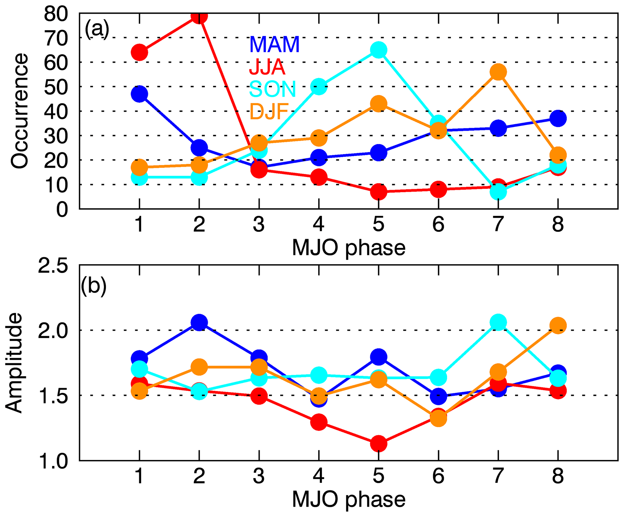
As seasonality is a basic feature of the MJO (Zhang and Dong, 2004), we first classify the MJO events during 2007–2010 into four seasons according to the MJO index from Wheeler and Hendon (2004) (Fig. 11). In total, 917 events with amplitude greater than one – i.e., (RMM12 + RMM22)0.5>1 – are selected to represent strong MJO. As shown in Fig. 11a, the occurrence of different MJO phases displays very strong seasonality. Specifically, more MJO events happen in Phases 1 and 2 in summer, while in fall, the MJO cases are concentrated in Phases 4, 5, and 6. When it moves to winter, the MJO tends to occur in Phase 7, while in spring, more cases occur in Phases 1 and 8. Although the MJO amplitude is relatively flat across different phases, the weakest amplitude occurs in summer, while it is stronger towards winter, which is consistent with the statements in previous studies (Adames et al., 2016; Zhang and Dong, 2004).
To investigate the spatial heterogeneity associated with the MJO, Fig. 12 shows the spatial distributions of all-sky Hσ over eight MJO phases. According to the spatial heterogeneity signatures derived in Sect. 3.1.5, the active MJO phase associated with deep convections and ice clouds is featured with small Hσ values. Areas surrounding the convective center are with relatively large Hσ values, indicating that the locations of suppressed MJO phase are associated with more liquid clouds. As displayed in Fig. 12, the Hσ pattern reveals well the propagation of MJO. That is, the center of convection associated with small Hσ is in the Indian Ocean in Phases 1 and 2, while the western Pacific and Maritime Continent display large Hσ as convection is suppressed. The small Hσ pattern approaches the Maritime Continent (indicated by the dashed red box in Fig. 12) in Phase 3 and centers at those regions in Phases 4, 5, and 6. After Phase 6, the convective center with small Hσ enters the western Pacific Ocean, and at the same time, Hσ becomes large over the Indian Ocean. Note that Phase 2 mainly occurs in summer, which relates to the boreal summer monsoon, so the Hσ pattern here is quite similar to that in summer shown in Fig. 8g2. Similarly, the Hσ pattern of Phase 5 is in concert with the seasonal pattern in fall (Fig. 8g3) due to a high chance of Phase 5 occurring in that season. The preference of geographical location of MJO, featured by the small Hσ, moves from north of the Equator in Phase 1 to south of the Equator in Phase 6, indicating the seasonal cycle of MJO location.
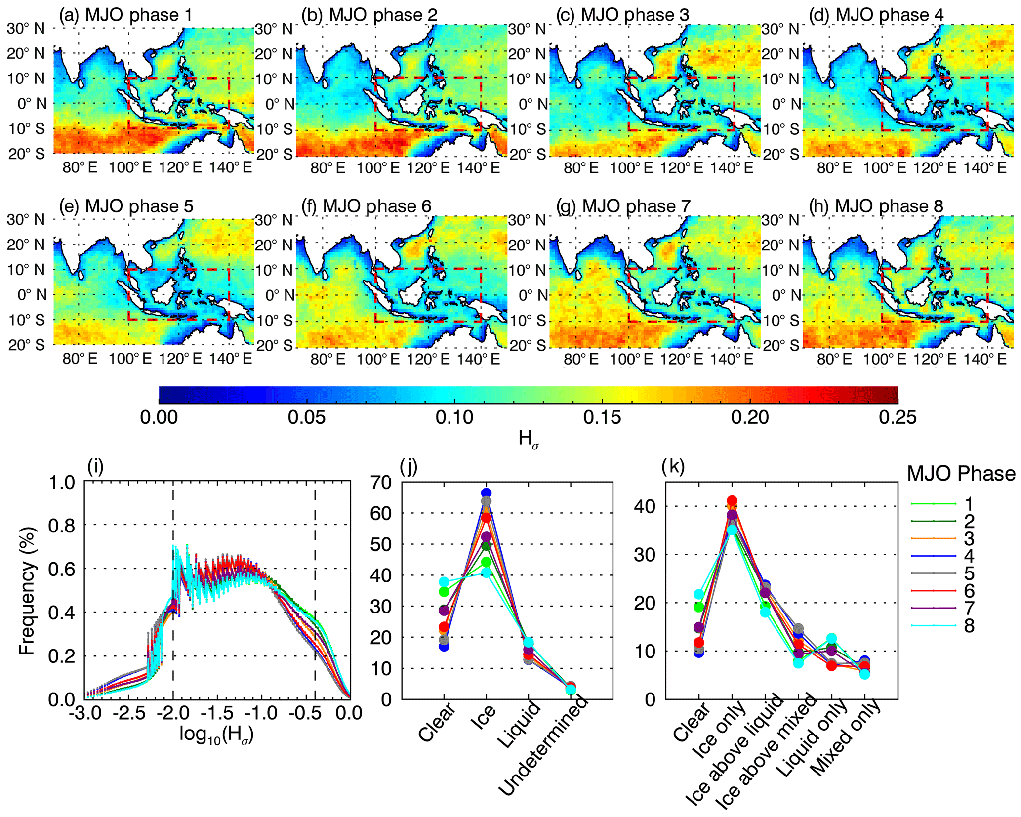
Figure 12Cloud phase characteristics in different MJO phases: (a–h) spatial distributions of all-sky Hσ derived from MYD06; (i) PDF of all-sky Hσ derived from MYD06 over the Maritime Continent (the dashed red box in each panel); (j) occurrence frequency of clear sky and ice, liquid, and undetermined clouds from MYD06 (unit: %); panel (k) is the same as (j) but for clear sky and five groups derived from the 2B-CLDCLASS-LIDAR product.
To investigate more details of how the Hσ pattern changes with cloud phase along with the MJO evolution, Fig. 12i shows the PDF of all-sky Hσ sampling over the Maritime Continent for the eight MJO phases from MODIS data. Two dashed lines from left to right indicate Hσ∼0.01 and Hσ∼0.4, which are close to the mode position of the Hσ PDF of CC clear sky and liquid-only clouds (Fig. 7a), respectively. Figure 12j and k show the average occurrence frequency of different cloud phases from the MYD06 and the 2B-CLDCLASS-LIDAR products in the same region. In Phase 8 (cyan) when suppressed MJO occurs over the Maritime Continent, the Hσ PDF shows the largest frequency (∼0.38 %) among all MJO phases at Hσ∼0.4 but the smallest frequency when Hσ<0.01 (Fig. 12i). This corresponds to the largest frequency of clear sky and liquid clouds among all MJO phases but the smallest frequency of ice clouds indicated by MODIS (Fig. 12j), and at the same time, ice-only, ice-above-liquid, and ice-above-mixed clouds from the 2B-CLDCLASS-LIDAR products occur the least frequently (Fig. 12k). In contrast, when active MJO phase is located over the Maritime Continent (Phases 4, 5), the Hσ PDF has the largest frequency at Hσ<0.01 and the smallest frequency at Hσ∼0.4, due to the frequent occurrence of ice or mixed clouds but less frequent occurrence of clear sky and liquid clouds.
Overall, more ice-contained clouds occurring during the active MJO phase results in smoother textures, i.e., small Hσ values, compared to the suppressed MJO phase. The eastward-propagating Hσ patterns vary with MJO, indicating that Hσ could be useful for MJO studies, such as serving as an observation-based parameter to track the MJO position. It can also serve as a basis for disentangling true space–time variability in cloud optical and microphysical properties associated with the MJO from space–time variability in the biases rooted in cloud retrievals from passive sensors that are caused by departures from the plane-parallel assumption (Di Girolamo et al., 2010).
3.3 Interannual variations: El Niño–Southern Oscillation
It is well known that ENSO dominates the interannual variability in precipitation and clouds over the western equatorial Pacific (As-Syakur et al., 2016; Park and Leovy, 2004; Reid et al., 2012), and accordingly, the observed broadband radiation at the TOA varies interannually as well (e.g., Loeb et al., 2012). Here we examine how the spectral radiances and spatial heterogeneity associated with cloud phase behave interannually.
The spatial distributions of the all-sky spatial heterogeneity (Hσ) anomaly is shown in Fig. 13 in El Niño and La Niña years based on the ENSO index and MODIS data from 2003 to 2017. Generally, all-sky Hσ anomaly is negative in La Niña years, indicating that more ice and mixed clouds occur in La Niña years causing the spatial heterogeneity to be more homogeneous than normal and vice versa in El Niño years. Also, the anomalies over the Maritime Continent tend to be stronger in winter and spring than in summer and fall (Fig. 13). This demonstrates that the Hσ varies with ENSO.
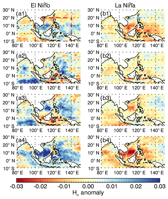
Figure 13Spatial heterogeneity anomaly in El Niño and La Niña years, from top to bottom for MAM, JJA, SON, and DJF.
Figure 14 displays the time series of monthly anomaly of clouds, radiances, and spatial heterogeneity for the areas indicated by the dashed red box in Fig. 13a1 – an area sensitive to ENSO signals. As displayed, ice clouds detected by MODIS show similar variations as MODIS all clouds with their anomalies ranging from −0.2 to 0.2, being positive in La Niña years and negative in El Niño years (Fig. 14b). The MODIS ice cloud anomaly correlates well with that of CC ice-only, ice-above-liquid, ice-above-mixed, and mixed-only clouds (Fig. 14d), with correlation coefficients greater than 0.70 (significant at the 99 % confidence level). Conversely, the anomaly of liquid cloud occurrence is positive (negative) in a El Niño (La Niña) year based on both the MODIS and CC data (Fig. 14b, d). Correspondingly, Hσ anomalies are observed to be negative in La Niña years due to the increase in ice-contained clouds and positive in El Niño years because ice-contained clouds decrease, exposing more liquid clouds (Fig. 14b, d). Moreover, the correlation coefficient between Hσ and the ENSO index is about 0.49 (significant at 99 % confidence level), further indicating that the change in spatial heterogeneity is associated with ENSO.

Figure 14ENSO index and monthly anomaly of cloud, spatial heterogeneity, and radiation in the region represented by the dashed red box in Fig. 13a1.
Note that negative (positive) anomaly of CC liquid-only or MODIS liquid clouds associated with La Niña (El Niño) phase does not mean that total liquid clouds occur less (more) in La Niña (El Niño) years. The overlying clouds can conceal liquid clouds to be observed from space by passive sensors or by lidar if the overlying clouds are optically thicker than 3. Unlike CC liquid-only or MODIS liquid clouds, the CC ice-above-liquid clouds occur abnormally high in La Niña years (Fig. 14d). When adding up the frequency of liquid-only and ice-above-liquid clouds (i.e., total CC liquid cloud frequency), the anomaly shows the relationship with ENSO is less evident than the liquid-only clouds (the subfigure in Fig. 14d). For example, through the La Niña phase in 2007 winter through 2008 spring, the anomaly of total CC liquid cloud occurrence is close to be zero, blurring its relationship with ENSO. Park and Leovy (2004) showed negative anomalies of low-level clouds during the positive ENSO phase using ship observations reported by the Extended Edited Cloud Report Archive (EECRA), i.e., less low-level clouds in El Niño years. While in our study, it is likely that MODIS data and 4-year CC data are insufficient to support the relationship between liquid cloud occurrence and ENSO over SEA.
Overall, the cloud phase varies interannually, as does Hσ, i.e., being smoother in La Niña years compared to El Niño years. Also, the time series of all-sky Hσ anomalies vary with ENSO, and it correlates well with that of R0.645 (, significant at 99 % confidence level) and BT11 (r∼0.8, significant at 99 % confidence level), indicating that Hσ can be one valuable observed parameter to investigate ENSO, including its basis for indicating the space–time variability, associated with ENSO, of the biases of cloud optical/microphysical properties retrieved from passive sensors, caused by departures from the plane-parallel assumption.
This work contributes to a series of studies that examine cloud vertical structures. Li et al. (2015) explored the vertical distributions of cloud types using the 2B-CLDCLASS-LIDAR data, while Oreopoulos et al. (2017) interpreted the overlap feature of high, middle, and low clouds. Considering the need for cloud phase information for improving GCMs (e.g., Cesana and Storelvmo, 2017), the current study focuses on investigating the characteristics of cloud vertical structures, spatial heterogeneity, and spectral radiances from the perspective of cloud phases over Southeast Asia. Utilizing the state-of-the-art CloudSat and CALIPSO (CC) observations, five cloud groups have been classified – ice-only, ice-above-liquid, ice-above-mixed, liquid-only, and mixed-only clouds – to capture the main vertical structures of cloud phases. By collocating the CC–MODIS data, the spectral and spatial heterogeneity signatures at the TOA of each CC cloud group have been examined. Seasonal, intraseasonal, and interannual variations in these cloud phase characteristics have also been shown in this work.
A general review on cloud spatial distributions and meteorology shows that the annual cloud occurrence frequency over SEA is about 81.4 %, being more frequent in summer (86.5 %) and less frequent in winter (78 %) based on the CC observations. Ice-only (28.6 %), ice-above-liquid (20.1 %), ice-above-mixed (9.3 %), and mixed-only (6.7 %) clouds, i.e., ice-contained clouds, preferentially occur in a warm, humid, and unstable environments and are associated with the seasonal movement of the monsoon and ITCZ. It is noted that ice-only and ice-above-liquid clouds are associated with similar upper-troposphere dynamics, i.e., comparable mean temperature, specific humidity, and static stability, while ice-above-mixed clouds occur in an environment with larger specific humidity at the upper troposphere. Liquid-only clouds appear frequently in winter and spring over southeastern China and the East China Sea where the lower troposphere is relatively cold, dry, and stable.
It is shown that ice clouds over SEA are thin with about 60 % and 80 % of samples with geometrical thickness smaller than 3.0 km and optical depth less than 3, respectively. Ice-only clouds have larger mean thickness (geometrical and optical) and Re than the ice layers above liquid or mixed clouds. Although there could exist sampling biases due to instrument limitations, a higher frequency of ice-only clouds at demonstrates that more ice-only clouds develop thicker than either the ice layers above liquid or mixed clouds. The tops of liquid-only clouds are on average lower than those of the liquid below ice clouds. As liquid-only clouds occur more frequently with increase in LTSS, their vertical development is likely to be inhibited. However, ice-above-liquid clouds more favorably distribute in a warm, humid, and unstable environment, which allows the underlying liquid clouds to grow deeper. The tops of mixed layers below ice clouds are primarily located at about 6 km. For mixed-only clouds, their tops are primarily at 16 km over ocean, but over land, a large fraction of samples have cloud top around 6 km. These results suggest that ice-above-mixed and mixed-only clouds over land are under development in the early afternoon.
We also show that distinct spatial heterogeneity exists between the five cloud groups. Ice-only, ice-above-mixed, and mixed-only clouds are usually homogeneous, i.e., small Hσ values. In contrast, liquid-only clouds show the largest Hσ among all cloud phase groups, being the most heterogeneous. Ice-above-liquid clouds have large but slightly smaller Hσ values than liquid-only clouds because the overlying homogenous and thin ice clouds slightly smooth the radiation emerging from the low-level liquid clouds. A typical Hσ value for clear sky is 0.01; however, clear-sky Hσ can be as large as 1, resulting from the increase in subpixel variability due to undetected liquid clouds in the MODIS and CC pixels. As large Hσ values are reported to be associated with the biases of cloud τ and Re derived from passive sensors (Di Girolamo et al., 2010; Zhang and Platnick, 2011), biases resulting from the plane-parallel assumption are expected to be larger for liquid than ice clouds. The seasonal patterns of all-sky Hσ show small values north of the Equator over the Indian and western Pacific oceans in summer but move southward in autumn and winter, being consistent with the seasonal shift of the ice-contained clouds.
A difference of cloud optical and micro- and macrophysical properties leads to distinct spectral features between the five cloud groups. The liquid-only clouds show zero R1.375, large reflectance ratio of the SWIR to the visible, high BTs, and negative BTD between 8.5 and 11 µm. Ice-only clouds in contrast show notable R1.375, a reflectance ratio generally smaller than 0.4, relatively low BTs, and more than 50 % of samples with positive BTD. Ice-above-liquid clouds behave more like ice-only clouds in the IR because these two cloud groups have similar BT11 and BTD PDFs, but ice-above-liquid clouds act more like liquid-only clouds in the SW spectrum due to their similar PDFs/CDFs of reflectance ratio. The average R1.375 of ice-above-liquid clouds, which is mainly contributed by the ice layers only, is smaller than that of ice-only clouds. Similarly, ice-above-liquid clouds have their average BT11 slightly larger than that of ice-only clouds. These results demonstrate that ice-only clouds are on average thicker than the ice layers above liquid clouds, being consistent with the conclusions derived from the CC observations. Mixed-only or ice-above-mixed clouds usually have a large R0.64, small reflectance ratio, low BT11, and positive BTD. It is also noted that the R0.645 and BT11 PDFs of ice-only, liquid-only, and ice-above-liquid clouds show their frequency peaks are nearly same as that of clear sky, revealing ubiquitous thin clouds over SEA.
Cloud phases together with their spectral and spatial heterogeneity features have also been examined in different MJO and ENSO phases. In the MJO active phase, more frequent ice-contained clouds contribute to a smooth MJO center. On both sides of the MJO convective center, large Hσ values are observed due to increase in liquid clouds and decrease in ice-contained clouds. Thus, the Hσ pattern reveals the eastward-propagating MJO. Similarly, the interannual variation in clouds over SEA is primarily due to the change in ice-contained clouds. Increased ice-contained clouds in La Niña years result in more homogeneous spatial heterogeneity, stronger R0.645, and lower BT11 and vice versa in El Niño years. The observed Hσ varies with the ENSO index with a correlation coefficient of 0.49 (significant at confidence level 0.99). The Hσ varying with the MJO and ENSO forms a basis for disentangling the true intraseasonal/interannual variability in cloud optical/microphysical properties from the space–time variability in cloud biases due to the plane-parallel assumption in cloud retrievals from passive sensors.
Finally, careful comparisons between model and observations can use Hσ as a measure of departure from the plane-parallel assumption in a manner similar to Loveridge and Davies (2019), where they used Hσ within their analysis in examining GCM clouds in different sectors of Southern Hemisphere cyclones. Hσ can also be used to gauge biases in other satellite products that are used in model evaluation (e.g., Gettelman et al., 2015; Song et al., 2018), such as cloud optical depth and effective radius, whose biases have been noted to covary with Hσ (Fu et al., 2019; Zhang et al., 2016).
Data used in this study are summarized in Table 1, and their availability is provided in the Acknowledgements.
YH and LDG conceived this study. YH analyzed the results and wrote the paper. LDG joined result discussions and refined this paper.
The authors declare that they have no conflict of interest.
We are grateful to Guangyu Zhao for his examination of clear-sky Hσ derived from ASTER and MODIS. We acknowledge the members of the CloudSat Data Processing Center who provide CloudSat products, including 2B-CLDCLASS-LIDAR, 2C-ICE, and ECMWF-AUX, available at http://www.cloudsat.cira.colostate.edu/ (CloudSat, 2020). The MODIS products, MYD021KM, MYD03, and MYD06, are obtained via the Level-1 and Atmosphere Archive & Distribution System (LAADS) Distributed Active Archive Center (DAAC), which is available at https://ladsweb.modaps.eosdis.nasa.gov/ (LAADS DAAC, 2020). We also thank the Bureau of Meteorology in Australia for offering the MJO index (available at http://www.bom.gov.au/climate/mjo/, RMM index, 2020) and NOAA Earth System Research Laboratory for providing the Multivariate ENSO index that can be downloaded from https://psl.noaa.gov/enso/mei/ (MEI, 2020).
This research has been supported by the Cloud, Aerosol and Monsoon Processes Philippines Experiment (CAMP2Ex) under NASA (grant no. 80NSSC18K0144).
This paper was edited by Corinna Hoose and reviewed by three anonymous referees.
Adames, Á. F., Wallace, J. M., and Monteiro, J. M.: Seasonality of the structure and propagation characteristics of the MJO, J. Atmos. Sci., 73, 3511–3526, https://doi.org/10.1175/JAS-D-15-0232.1, 2016.
As-Syakur, A. R., Osawa, T., Miura, F., Nuarsa, I. W., Ekayanti, N. W., Dharma, I. G. B. S., Adnyana, I. W. S., Arthana, I. W., and Tanaka, T.: Maritime Continent rainfall variability during the TRMM era: The role of monsoon, topography and El Niño Modoki, Dyn. Atmos. Ocean., 75, 58–77, https://doi.org/10.1016/j.dynatmoce.2016.05.004, 2016.
Barnes, W. L., Pagano, T. S., and Salomonson, V. V.: Prelaunch characteristics of the moderate resolution, IEEE T. Geosci. Remote Sens., 36, 1088–1100, 1998.
Baum, B. A., Menzel, W. P., Frey, R. A., Tobin, D. C., Holz, R. E., Ackerman, S. A., Heidinger, A. K., and Yang, P.: MODIS cloud-top property refinements for collection 6, J. Appl. Meteorol. Clim., 51, 1145–1163, https://doi.org/10.1175/JAMC-D-11-0203.1, 2012.
Berry, E., Mace, G. G., and Gettelman, A.: Using A-Train observations to evaluate cloud occurrence and radiative effects in the Community Atmosphere Model during the Southeast Asia summer monsoon, J. Climate, 32, 4145–4165, https://doi.org/10.1175/jcli-d-18-0693.1, 2019.
Bouet, C., Szczap, F., Leriche, M., and Benassi, A.: What is the effect of cloud inhomogeneities on actinic fluxes and chemical species concentrations?, Geophys. Res. Lett., 33, L01818, https://doi.org/10.1029/2005GL024727, 2006.
Cesana, G.: Using in situ airborne measurements to evaluate three cloud phase products derived from CALIPSO, J. Geophys. Res.-Atmos., 121, 5788–5808, https://doi.org/10.1002/2014JD022963, 2016.
Cesana, G. and Storelvmo, T.: Improving climate projections by understanding how cloud phase affects radiation, J. Geophys. Res.-Atmos., 122, 4594–4599, https://doi.org/10.1002/2017JD026927, 2017.
Cesana, G. and Waliser, D. E.: Characterizing and understanding systematic biases in the vertical structure of clouds in CMIP5/CFMIP2 models, Geophys. Res. Lett., 43, 10538–10546, https://doi.org/10.1002/2016GL070515, 2016.
Cesana, G., Waliser, D. E., Jiang, X., and Li, J. L. F.: Multimodel evaluation of cloud phase transition using satellite and reanalysis data, J. Geophys. Res.-Atmos., 120, 7871–7892, https://doi.org/10.1002/2014JD022932, 2015.
Cesana, G., Waliser, D. E., Henderson, D., L'Ecuyer, T. S., Jiang, X., and Li, J.-L. F.: The vertical structure of radiative heating rates: A multimodel evaluation using A-train satellite observations, J. Climate, 32, 1573–1590, https://doi.org/10.1175/jcli-d-17-0136.1, 2018.
Cesana, G., Del Genio, A. D., and Chepfer, H.: The Cumulus And Stratocumulus CloudSat-CALIPSO Dataset (CASCCAD), Earth Syst. Sci. Data, 11, 1745–1764, https://doi.org/10.5194/essd-11-1745-2019, 2019.
Cho, H. M., Nasiri, S. L., and Yang, P.: Application of CALIOP measurements to the evaluation of cloud phase derived from MODIS infrared channels, J. Appl. Meteorol. Clim., 48, 2169–2180, https://doi.org/10.1175/2009JAMC2238.1, 2009.
Cho, H. M., Zhang, Z., Meyer, K., Lebsock, M., Platnick, S., Ackerman, A. S., Di Girolamo, L., Labonnote, L. C., Cornet, C., Riedi, J., and Holz, R. E.: Frequency and causes of failed MODIS cloud property retrievals for liquid phase clouds over global oceans, J. Geophys. Res.-Atmos., 120, 4132–4154, https://doi.org/10.1002/2015JD023161, 2015.
Christensen, M. W., Carrió, G. G., Stephens, G. L., and Cotton, W. R.: Radiative impacts of free-tropospheric clouds on the properties of marine stratocumulus, J. Atmos. Sci., 70, 3102–3118, https://doi.org/10.1175/JAS-D-12-0287.1, 2013.
CloudSat: CloudSat Data Processing Center, available at: http://www.cloudsat.cira.colostate.edu/, last access: 10 July 2020.
Cronk, H. and Partain, P.: CloudSat ECMWF-AUX auxillary data product process description and interface control document, 15 pp., available at: http://www.cloudsat.cira.colostate.edu/sites/default/files/products/files/ECMWF-AUX_PDICD.P_R05.rev0_.pdf (last access: 10 July 2020), 2017.
Deng, M., Mace, G. G., Wang, Z., and Okamoto, H.: Tropical composition, cloud and climate coupling experiment validation for cirrus cloud profiling retrieval using cloudsat radar and CALIPSO lidar, J. Geophys. Res., 115, D00J15, https://doi.org/10.1029/2009JD013104, 2010.
Deng, M., Mace, G. G., Wang, Z., and Lawson, R. P.: Evaluation of several A-train ice cloud retrieval products with in situ measurements collected during the SPARTICUS campaign, J. Appl. Meteorol. Clim., 52, 1014–1030, https://doi.org/10.1175/JAMC-D-12-054.1, 2013.
Di Girolamo, L., Liang, L., and Platnick, S.: A global view of one-dimensional solar radiative transfer through oceanic water clouds, Geophys. Res. Lett., 37, L18809, https://doi.org/10.1029/2010GL044094, 2010.
Di Girolamo, L., Holz, R., Reid, J., Tanelli, S., and Van Den Heaver, S.: Cloud and Aerosol Monsoonal Processes-Philippines Experiment (CAMP2Ex), 1–30, available at: https://espo.nasa.gov/CAMP2Ex_White_Paper (last access: 10 July 2020), 2018.
Dolinar, E. K., Dong, X., Xi, B., Jiang, J. H., and Su, H.: Evaluation of CMIP5 simulated clouds and TOA radiation budgets using NASA satellite observations, Clim. Dynam., 44, 2229–2247, https://doi.org/10.1007/s00382-014-2158-9, 2014.
Eliasson, S., Buehler, S. A., Milz, M., Eriksson, P., and John, V. O.: Assessing observed and modelled spatial distributions of ice water path using satellite data, Atmos. Chem. Phys., 11, 375–391, https://doi.org/10.5194/acp-11-375-2011, 2011.
Fu, D., Di Girolamo, L., Liang, L., and Zhao, G.: Regional Biases in MODIS Marine Liquid Water Cloud Drop Effective Radius Deduced Through Fusion With MISR, J. Geophys. Res.-Atmos., 124, 13182–13196, https://doi.org/10.1029/2019JD031063, 2019.
Gettelman, A., Morrison, H., Santos, S., Bogenschutz, P. and Caldwell, P. M.: Advanced two-moment bulk microphysics for global models. Part II: Global model solutions and aerosol-cloud interactions, J. Climate, 28, 1288–1307, https://doi.org/10.1175/JCLI-D-14-00103.1, 2015.
Grise, K. M., Thompson, D. W. J., and Birner, T.: A global survey of static stability in the stratosphere and upper troposphere, J. Climate, 23, 2275–2292, https://doi.org/10.1175/2009JCLI3369.1, 2010.
Grose, M. R., Brown, J. N., Narsey, S., Brown, J. R., Murphy, B. F., Langlais, C., Gupta, A. Sen, Moise, A. F., and Irving, D. B.: Assessment of the CMIP5 global climate model simulations of the western tropical Pacific climate system and comparison to CMIP3, Int. J. Climatol., 34, 3382–3399, https://doi.org/10.1002/joc.3916, 2014.
Haladay, T. and Stephens, G.: Characteristics of tropical thin cirrus clouds deduced from joint CloudSat and CALIPSO observations, J. Geophys. Res., 114, D00A25, https://doi.org/10.1029/2008JD010675, 2009.
Ham, S.-H., Kato, S., Barker, H. W., Rose, F. G., and Sun-Mack, S.: Improving the modelling of short-wave radiation through the use of a 3D scene construction algorithm, Q. J. Roy. Meteor. Soc., 141, 1870–1883, https://doi.org/10.1002/qj.2491, 2015.
Hong, Y. and Liu, G.: The characteristics of ice cloud properties derived from CloudSat and CALIPSO measurements, J. Climate, 28, 3880–3901, https://doi.org/10.1175/JCLI-D-14-00666.1, 2015.
Hong, Y., Liu, G., and Li, J.-L. F.: Assessing the radiative effects of global ice clouds based on CloudSat and CALIPSO measurements, J. Climate, 29, 7651–7674, https://doi.org/10.1175/JCLI-D-15-0799.1, 2016.
Hu, Y., Winker, D., Vaughan, M., Lin, B., Omar, A., Trepte, C., Flittner, D., Yang, P., Nasiri, S. L., Baum, B., Sun, W., Liu, Z., Wang, Z., Young, S., Stamnes, K., Huang, J., Kuehn, R., and Holz, R.: CALIPSO/CALIOP cloud phase discrimination algorithm, J. Atmos. Ocean. Tech., 26, 2293–2309, https://doi.org/10.1175/2009JTECHA1280.1, 2009.
Hu, Y., Rodier, S., Xu, K. M., Sun, W., Huang, J., Lin, B., Zhai, P., and Josset, D.: Occurrence, liquid water content, and fraction of supercooled water clouds from combined CALIOP/IIR/MODIS measurements, J. Geophys. Res., 115, D00H34, https://doi.org/10.1029/2009JD012384, 2010.
Jiang, J. H., Su, H., Zhai, C., Perun, V. S., Del Genio, A., Nazarenko, L. S., Donner, L. J., Horowitz, L., Seman, C., Cole, J., Gettelman, A., Ringer, M. A., Rotstayn, L., Jeffrey, S., Wu, T., Brient, F., Dufresne, J.-L., Kawai, H., Koshiro, T., Watanabe, M., LÉcuyer, T. S., Volodin, E. M., Iversen, T., Drange, H., Mesquita, M. D. S., Read, W. G., Waters, J. W., Tian, B., Teixeira, J., and Stephens, G. L.: Evaluation of cloud and water vapor simulations in CMIP5 climate models using NASA “A-Train” satellite observations, J. Geophys. Res., 117, D14105, https://doi.org/10.1029/2011jd017237, 2012.
Kay, J. E., Bourdages, L., Miller, N. B., Morrison, A., Yettella, V., Chepfer, H., and Eaton, B.: Evaluating and improving cloud phase in the Community Atmosphere Model version 5 using spaceborne lidar observations, J. Geophys. Res.-Atmos., 121, 4162–4176, https://doi.org/10.1002/2015JD024699, 2016.
King, M. D., Kaufman, Y. J., Menzel, W. P., and Tanré, D.: Remote sensing of cloud, aerosol, and water vapor properties from the Moderate Resolution Imaging Spectrometer (MODIS), IEEE T. Geosci. Remote Sens., 30, 2–27, https://doi.org/10.1109/36.124212, 1992.
King, M. D., Platnick, S., Menzel, W. P., Ackerman, S. A., and Hubanks, P. A.: Spatial and temporal distribution of clouds observed by MODIS onboard the Terra and Aqua satellites, IEEE T. Geosci. Remote Sens., 51, 3826–3852, https://doi.org/10.1109/TGRS.2012.2227333, 2013.
Klein, S. A. and Hartmann, D.: The seasonal cycle of low startiform clouds, J. Climate, 6, 1587–1606, https://doi.org/10.1175/1520-0442(1993)006<1587:TSCOLS>2.0.CO;2, 1993.
Knutson, T. R., Weickmann, K. M., and Kutzbach, J. E.: Global-scale intraseasonal oscillations of outgoing longwave radiation and 250 mb zonal wind during northern hemisphere summer, Mon. Weather Rev., 114, 605–623, 1986.
LAADS DAAC: Level-1 Atmosphere Archive & Distribution System Distributed Active Archive Center for MODIS data, available at: https://ladsweb.modaps.eosdis.nasa.gov/, last access: 10 July 2020.
Leahy, L. V., Wood, R., Charlson, R. J., Hostetler, C. A., Rogers, R. R., Vaughan, M. A., and Winker, D. M.: On the nature and extent of optically thin marine low clouds, J. Geophys. Res., 117, D22201, https://doi.org/10.1029/2012JD017929, 2012.
Li, J., Yi, Y., Minnis, P., Huang, J., Yan, H., Ma, Y., Wang, W., and Kirk Ayers, J.: Radiative effect differences between multi-layered and single-layer clouds derived from CERES, CALIPSO, and CloudSat data, J. Quant. Spectrosc. Ra., 112, 361–375, https://doi.org/10.1016/j.jqsrt.2010.10.006, 2011.
Li, J., Huang, J., Stamnes, K., Wang, T., Lv, Q., and Jin, H.: A global survey of cloud overlap based on CALIPSO and CloudSat measurements, Atmos. Chem. Phys., 15, 519–536, https://doi.org/10.5194/acp-15-519-2015, 2015.
Li, J.-L. F., Waliser, D. E., Stephens, G., Lee, S., L'Ecuyer, T., Kato, S., Loeb, N., and Ma, H.-Y.: Characterizing and understanding radiation budget biases in CMIP3/CMIP5 GCMs, contemporary GCM, and reanalysis, J. Geophys. Res.-Atmos., 118, 8166–8184, https://doi.org/10.1002/jgrd.50378, 2013.
Li, Y., Thompson, D. W. J., Stephens, G. L., and Bony, S.: A global survey of the instantaneous linkages between cloud vertical structure and large-scale climate, J. Geophys. Res.-Atmos., 119, 3770–3792, https://doi.org/10.1002/2013JD020669, 2014.
Liang, L., Di Girolamo, L., and Platnick, S.: View-angle consistency in reflectance, optical thickness and spherical albedo of marine water-clouds over the northeastern Pacific through MISR-MODIS fusion, Geophys. Res. Lett., 36, L09811, https://doi.org/10.1029/2008GL037124, 2009.
Liang, L., Di Girolamo, L., and Sun, W.: Bias in MODIS cloud drop effective radius for oceanic water clouds as deduced from optical thickness variability across scattering angles, J. Geophys. Res.-Atmos., 120, 7661–7681, https://doi.org/10.1002/2015JD023256, 2015.
Lin, N. H., Tsay, S. C., Maring, H. B., Yen, M. C., Sheu, G. R., Wang, S. H., Chi, K. H., Chuang, M. T., Ou-Yang, C. F., Fu, J. S., Reid, J. S., Lee, C. Te, Wang, L. C., Wang, J. L., Hsu, C. N., Sayer, A. M., Holben, B. N., Chu, Y. C., Nguyen, X. A., Sopajaree, K., Chen, S. J., Cheng, M. T., Tsuang, B. J., Tsai, C. J., Peng, C. M., Schnell, R. C., Conway, T., Chang, C. T., Lin, K. S., Tsai, Y. I., Lee, W. J., Chang, S. C., Liu, J. J., Chiang, W. L., Huang, S. J., Lin, T. H., and Liu, G. R.: An overview of regional experiments on biomass burning aerosols and related pollutants in Southeast Asia: From BASE-ASIA and the Dongsha Experiment to 7-SEAS, Atmos. Environ., 78, 1–19, https://doi.org/10.1016/j.atmosenv.2013.04.066, 2013.
Liou, K.-N.: Influence of cirrus clouds on weather and climate processes: A global perspective, Mon. Weather Rev., 114, 1167–1199, https://doi.org/10.1175/1520-0493(1986)114<1167:IOCCOW>2.0.CO;2, 1986.
Loeb, N. G. and Davies, R.: Observational evidence of plane parallel model biases?: Apparent dpendence of cloud optical depth on solar zenith angle, J. Geophys. Res., 101, 1621–1634, 1996.
Loeb, N. G. and Davies, R.: Angular dependence of observed reflectances: A comparison with plane parallel theory, J. Geophys. Res.-Atmos., 102, 6865–6881, https://doi.org/10.1029/96JD03586, 1997.
Loeb, N. G., Kato, S., Su, W., Wong, T., Rose, F. G., Doelling, D. R., Norris, J. R., and Huang, X.: Advances in understanding top-of-atmosphere radiation variability from satellite observations, Surv. Geophys., 33, 359–385, https://doi.org/10.1007/s10712-012-9175-1, 2012.
Loveridge, J. and Davies, R.: Cloud heterogeneity in the marine midlatitudes: Dependence on large-scale meteorology and implications for general circulation models, J. Geophys. Res.-Atmos., 124, 3448–3463, https://doi.org/10.1029/2018JD029826, 2019.
Mace, G. G., Zhang, Q., Vaughan, M., Marchand, R., Stephens, G., Trepte, C., and Winker, D.: A description of hydrometeor layer occurrence statistics derived from the first year of merged Cloudsat and CALIPSO data, J. Geophys. Res., 114, D00A26, https://doi.org/10.1029/2007JD009755, 2009.
Madden, R. A. and Julian, P. R.: Detection of a 40–50 Day Oscillation in the Zonal Wind in the Tropical Pacific, J. Atmos. Sci., 28, 702–708, https://doi.org/10.1175/1520-0469(1971)028<0702:DOADOI>2.0.CO;2, 1971.
Marchant, B., Platnick, S., Meyer, K., Arnold, G. T., and Riedi, J.: MODIS Collection 6 shortwave-derived cloud phase classification algorithm and comparisons with CALIOP, Atmos. Meas. Tech., 9, 1587–1599, https://doi.org/10.5194/amt-9-1587-2016, 2016.
Marshak, A. and Davis, A. B.: Horizontal fluxes and radiative smoothing, in: 3D Radiative Transfer in Cloudy Atmospheres, 543–586, Springer, Berlin, Heidelberg, 2005.
Marshak, A., Platnick, S., Várnai, T., Wen, G., and Cahalan, R. F.: Impact of three-dimensional radiative effects on satellite retrievals of cloud droplet sizes, J. Geophys. Res., 111, D09207, https://doi.org/10.1029/2005JD006686, 2006.
Matus, A. V. and L'Ecuyer, T. S.: The role of cloud phase in Earth's radiation budget, J. Geophys. Res.-Atmos., 122, 2559–2578, https://doi.org/10.1002/2016JD025951, 2017.
McFarquhar, G. M., Heymsfield, A. J., Spinhirne, J., and Hart, B.: Thin and subvisual tropopause tropical cirrus: Observations and radiative impacts, J. Atmos. Sci., 57, 1841–1853, https://doi.org/10.1175/1520-0469(2000)057<1841:TASTTC>2.0.CO;2, 2000.
MEI: Multivariate ENSO Index, Version 2, available at: https://psl.noaa.gov/enso/mei/, last access: 10 July 2020.
Nesbitt, S. W. and Zipser, E. J.: The diurnal cycle of rainfall and convective intensity according to three years of TRMM measurements, J. Climate, 16, 1456–1475, https://doi.org/10.1175/1520-0442-16.10.1456, 2003.
O'Hirok, W. and Gautier, C.: The impact of model resolution on differences between independent column approximation and monte carlo estimates of shortwave surface irradiance and atmospheric heating rate, J. Atmos. Sci., 62, 2939–2951, https://doi.org/10.1175/jas3519.1, 2005.
Oreopoulos, L., Cho, N., and Lee, D.: New insights about cloud vertical structure from CloudSat and CALIPSO observations, J. Geophys. Res.-Atmos., 122, 9280–9300, https://doi.org/10.1002/2017JD026629, 2017.
Park, S. and Leovy, C. B.: Marine low-cloud anomalies associated with ENSO, J. Climate, 17, 3448–3469, https://doi.org/10.1175/1520-0442(2004)017<3448:MLAAWE>2.0.CO;2, 2004.
Pincus, R., Platnick, S., Ackerman, S. A., Hemler, R. S., and Patrick Hofmann, R. J.: Reconciling simulated and observed views of clouds: MODIS, ISCCP, and the limits of instrument simulators, J. Climate, 25, 4699–4720, https://doi.org/10.1175/JCLI-D-11-00267.1, 2012.
Platnick, S., King, M. D., Ackerman, S. A., Menzel, W. P., Baum, B. A., Riédi, J. C., and Frey, R. A.: The MODIS cloud products?: Algorithms and examples from Terra, IEEE T. Geosci. Remote Sens., 41, 459–473, https://doi.org/10.1109/TGRS.2002.808301, 2003.
Reid, J. S., Xian, P., Hyer, E. J., Flatau, M. K., Ramirez, E. M., Turk, F. J., Sampson, C. R., Zhang, C., Fukada, E. M., and Maloney, E. D.: Multi-scale meteorological conceptual analysis of observed active fire hotspot activity and smoke optical depth in the Maritime Continent, Atmos. Chem. Phys., 12, 2117–2147, https://doi.org/10.5194/acp-12-2117-2012, 2012.
Reid, J. S., Hyer, E. J., Johnson, R. S., Holben, B. N., Yokelson, R. J., Zhang, J., Campbell, J. R., Christopher, S. A., Di Girolamo, L., Giglio, L., Holz, R. E., Kearney, C., Miettinen, J., Reid, E. A., Turk, F. J., Wang, J., Xian, P., Zhao, G., Balasubramanian, R., Chew, B. N., Janjai, S., Lagrosas, N., Lestari, P., Lin, N. H., Mahmud, M., Nguyen, A. X., Norris, B., Oanh, N. T. K., Oo, M., Salinas, S. V., Welton, E. J., and Liew, S. C.: Observing and understanding the Southeast Asian aerosol system by remote sensing: An initial review and analysis for the Seven Southeast Asian Studies (7SEAS) program, Atmos. Res., 122, 403–468, https://doi.org/10.1016/j.atmosres.2012.06.005, 2013.
Riley, E. M., Mapes, B. E., and Tulich, S. N.: Clouds associated with the Madden–Julian Oscillation: A new perspective from CloudSat, J. Atmos. Sci., 68, 3032–3051, https://doi.org/10.1175/JAS-D-11-030.1, 2011.
RMM index: Real-Time Multivariate MJO Index, available at: http://www.bom.gov.au/climate/mjo/, last access: 10 July 2020.
Ross, A. D., Holz, R. E., Quinn, G., Reid, J. S., Xian, P., Turk, F. J., and Posselt, D. J.: Exploring the first aerosol indirect effect over Southeast Asia using a 10-year collocated MODIS, CALIOP, and model dataset, Atmos. Chem. Phys., 18, 12747–12764, https://doi.org/10.5194/acp-18-12747-2018, 2018.
Sassen, K. and Wang, Z.: Classifying clouds around the globe with the CloudSat radar: 1-year of results, Geophys. Res. Lett., 35, L04805, https://doi.org/10.1029/2007GL032591, 2008.
Sassen, K., Wang, Z., and Liu, D.: Global distribution of cirrus clouds from CloudSat/Cloud-Aerosol Lidar and Infrared Pathfinder Satellite Observations (CALIPSO) measurements, J. Geophys. Res., 113, D00A12, https://doi.org/10.1029/2008JD009972, 2008.
Savtchenko, A., Ouzounov, D., Ahmad, S., Acker, J., Leptoukh, G., Koziana, J., and Nickless, D.: Terra and Aqua MODIS products available from NASA GES DAAC, Adv. Space Res., 34, 710–714, https://doi.org/10.1016/j.asr.2004.03.012, 2004.
Song, H., Zhang, Z., Ma, P. L., Ghan, S. J., and Wang, M.: An evaluation of marine boundary layer cloud property simulations in the Community Atmosphere Model using satellite observations: Conventional subgrid parameterization versus CLUBB, J. Climate, 31, 2299–2320, https://doi.org/10.1175/JCLI-D-17-0277.1, 2018.
Song, S., Schmidt, K. S., Pilewskie, P., King, M. D., Heidinger, A. K., Walther, A., Iwabuchi, H., Wind, G., and Coddington, O. M.: The spectral signature of cloud spatial structure in shortwave irradiance, Atmos. Chem. Phys., 16, 13791–13806, https://doi.org/10.5194/acp-16-13791-2016, 2016.
Stephens, G., Winker, D., Pelon, J., Trepte, C., Vane, D., Yuhas, C., L'Ecuyer, T., and Lebsock, M.: Cloudsat and CALIPSO within the A-train: Ten years of actively observing the earth system, B. Am. Meteorol. Soc., 99, 569–581, https://doi.org/10.1175/BAMS-D-16-0324.1, 2018.
Stephens, G. L., Vane, D. G., Boain, R. J., Mace, G. G., Sassen, K., Wang, Z., Illingworth, A. J., O'Connor, E. J., Rossow, W. B., Durden, S. L., Miller, S. D., Austin, R. T., Benedetti, A., and Mitrescu, C.: The cloudsat mission and the A-Train: A new dimension of space-based observations of clouds and precipitation, B. Am. Meteorol. Soc., 83, 1771–1790, https://doi.org/10.1175/BAMS-83-12-1771, 2002.
Stephens, G. L., Vane, D. G., Tanelli, S., Im, E., Durden, S., Rokey, M., Reinke, D., Partain, P., Mace, G. G., Austin, R., L'Ecuyer, T., Haynes, J., Lebsock, M., Suzuki, K., Waliser, D., Wu, D., Kay, J., Gettelman, A., Wang, Z., and Marchand, R.: CloudSat mission: Performance and early science after the first year of operation, J. Geophys. Res., 113, D00A18, https://doi.org/10.1029/2008JD009982, 2008.
Waliser, D. E., Li, J.-L. F., Woods, C. P., Austin, R. T., Bacmeister, J., Chern, J., Del Genio, A., Jiang, J. H., Kuang, Z., Meng, H., Minnis, P., Platnick, S., Rossow, W. B., Stephens, G. L., Sun-Mack, S., Tao, W.-K., Tompkins, A. M., Vane, D. G., Walker, C., and Wu, D.: Cloud ice: A climate model challenge with signs and expectations of progress, J. Geophys. Res., 114, D00A21, https://doi.org/10.1029/2008JD010015, 2009.
Wang, Z.: CloudSat 2B-CLDCLASS-LIDAR Product Process Description and Interface Control Document, 1–59, available at: http://www.cloudsat.cira.colostate.edu/sites/default/files/products/files/2B-CLDCLASS-LIDAR_PDICD.P1_R05.rev0_.pdf (last access: 10 July 2020), 2019.
Wang, Z. and Sassen, K.: Cloud type and macrophysical property retrieval using multiple remote sensors, J. Appl. Meteorol., 40, 1665–1682, https://doi.org/10.1175/1520-0450(2001)040<1665:CTAMPR>2.0.CO;2, 2001.
Wang, Z., Vane, D., and Staphens, G.: Level 2 Combined Radar and Lidar Cloud Scenario Classification Product Process Description and Interface Control document, available at: http://www.cloudsat.cira.colostate.edu/sites/default/files/products/files/2B-CLDCLASS-LIDAR_PDICD.P_R04.20120522.pdf (last access: 10 July 2020), 2012.
Wheeler, M. C. and Hendon, H. H.: An all-season real-time multivariate MJO index?: Development of an index for monitoring and prediction, Mon. Weather Rev., 132, 1917–1932, 2004.
Winker, D. M., Pelon, J. R., and McCormick, M. P.: The CALIPSO mission: Spaceborne lidar for observation of aerosols and clouds, Lidar Remote Sens. Ind. Environ. Monit. III, 4893, 1–11, https://doi.org/10.1117/12.466539, 2003.
Wolter, K. and Timlin, M. S.: Monitoring ENSO in COADS with a seasonality adjusted principal component index, in: Proc. of the 17th Climate Diagnostics Workshop, Norman, OK, NOAA/NMC/CAC, NSSL, Oklahoma Clim. Survey, CIMMS and the School of Meteor., Univ. of Oklahoma, 52–57, 1993.
Wolter, K. and Timlin, M. S.: Measuring the strength of ENSO events: How does 1997/1998 rank?, Weather, 53, 315–324, 1998.
Wolters, E. L. A., Roebeling, R. A., and Feijt, A. J.: Evaluation of cloud-phase retrieval methods for SEVIRI on Meteosat-8 using ground-based lidar and cloud radar data, J. Appl. Meteorol. Clim., 47, 1723–1738, https://doi.org/10.1175/2007JAMC1591.1, 2008.
Yang, P., Liou, K. N., Wyser, K., and Mitchell, D.: Parameterization of the scattering and absorption properties of individual ice crystals, J. Geophys. Res., 105, 4699–4718, https://doi.org/10.1029/1999JD900755, 2000.
Yeh, T. C.: Some aspects of the thermal influences of the Qinghai-Tibetan plateau on the atmospheric circulation, Arch. Meteorol. Geophy. A, 31, 205–220, https://doi.org/10.1007/BF02258032, 1982.
Yoshida, R., Okamoto, H., Hagihara, Y., and Ishimoto, H.: Global analysis of cloud phase and ice crystal orientation from Cloud-Aerosol Lidar and Infrared Pathfinder Satellite Observation (CALIPSO) data using attenuated backscattering and depolarization ratio, J. Geophys. Res.-Atmos., 115, 1–12, https://doi.org/10.1029/2009JD012334, 2010.
Yuan, T. and Oreopoulos, L.: On the global character of overlap between low and high clouds, Geophys. Res. Lett., 40, 5320–5326, doi:10.1002/grl.50871, 2013.
Zhang, C.: Madden-Julian Oscillation, Rev. Geophys., 43, RG2003, https://doi.org/10.1029/2004RG000158, 2005.
Zhang, C. and Dong, M.: Seasonality in the Madden-Julian oscillation, J. Climate, 17, 3169–3180, https://doi.org/10.1175/1520-0442(2004)017<3169:SITMO>2.0.CO;2, 2004.
Zhang, D., Wang, Z., and Liu, D.: A global view of midlevel liquid-layer topped stratiform cloud distribution and phase partition from CALIPSO and CloudSat measurements, J. Geophys. Res., 115, D00H13, https://doi.org/10.1029/2009JD012143, 2010.
Zhang, Z. and Platnick, S.: An assessment of differences between cloud effective particle radius retrievals for marine water clouds from three MODIS spectral bands, J. Geophys. Res.-Atmos., 116, D20215, https://doi.org/10.1029/2011JD016216, 2011.
Zhang, Z., Werner, F., Cho, H.-M., Wind, G., Platnick, S., Ackerman, A. S., Di Girolamo, L., Marshak, A., and Meyer, K.: A framework based on 2-D Taylor expansion for quantifying the impacts of subpixel reflectance variance and covariance on cloud optical thickness and effective radius retrievals based on the bispectral method, J. Geophys. Res.-Atmos., 121, 7007–7025, https://doi.org/10.1002/2016JD024837, 2016.
Zhao, G. and Di Girolamo, L.: Cloud fraction errors for trade wind cumuli from EOS-Terra instruments, Geophys. Res. Lett., 33, L20802, https://doi.org/10.1029/2006GL027088, 2006.
Zhao, G., Di Girolamo, L., Diner, D. J., Bruegge, C. J., Mueller, K. J., and Wu, D. L.: Regional changes in Earth's color and texture as observed from space over a 15-year period, IEEE T. Geosci. Remote Sens., 54, 4240–4249, https://doi.org/10.1109/TGRS.2016.2538723, 2016.
Zhao, W., Peng, Y., Wang, B., Yi, B., Lin, Y., and Li, J.: Comparison of three ice cloud optical schemes in climate simulations with community atmospheric model version 5, Atmos. Res., 204, 37–53, https://doi.org/10.1016/j.atmosres.2018.01.004, 2018.