2.1 Observational data from ICE-L

We use data from various instruments on board the National Science Foundation (NSF) C-130 aircraft for information about aerosol, cloud, and ice populations in the mixed-phase clouds observed in RF03 of the ICE-L campaign. Details on the instrumentation can be found in Heymsfield et al. (2011) for hydrometeor and aerosol size distributions and Pratt et al. (2010) for the aerosol chemical composition. Here we focus on a wave cloud observed on 16 November 2007 (RF03), for which observations from three different altitudes are available within a time interval of roughly 40 min. For the model evaluation, we use the King liquid water probe for total liquid water content, the 2D-C and the 2D-S probe for ice number concentrations and estimated ice water content, the CDP (cloud droplet probe) for cloud droplet number concentrations, the tuneable diode laser hygrometer (TDL) for humidity measurements, the counterflow virtual impactor (CVI) for total water content, and aerosol size distributions from the ultra-high sensitivity aerosol spectrometer (UHSAS) for size-resolved number concentrations. The data from 2D-C and 2D-S are restricted to particles larger than 50 µm. The small threshold particle size for the 2D-C is justified by the good agreement between ice crystal number concentrations from the 2D-S and 2D-C. Shattering in wave clouds is very likely not a large issue due to the predominantly small size of the ice crystals. As in Field et al. (2012) we correct the TDL humidity such that it is consistent with water saturation in the regions with a liquid water content (from the King liquid water probe) larger than 0.02 g m⁻³. Further details on the data and their postprocessing can be found in Field et al. (2012).

2.2 The Unified Model

We use the Unified Model (UM), the numerical weather prediction model developed by the Met Office and used for operational forecasting in the UK, to conduct simulations of the wave cloud observed during research flight 3 of the ICE-L campaign (16 November 2007). A global simulation (UM vn10.8, GA6 configuration, N512 resolution; Walters et al., 2017) starting from the operational analysis at 12:00 UTC on 16 November 2007 provides the initial and lateral boundary conditions for regional model simulations. Two regional nests are used, the first with a horizontal grid spacing of 1 km and the second with a grid spacing of 250 m. Both nests are centred at the location of the observed wave cloud (42.12^∘ N, −105.10^∘ E). The analysis presented in this paper focuses on the innermost nest. In the vertical we use a stretched vertical coordinate system with 140 levels, which provides a vertical resolution of 130–200 m at the altitude of the observed cloud. Mass conservation is enforced in the regional simulations (Aranami et al., 2014, 2015), and sub-grid-scale turbulent processes are represented with a 3D Smagorinsky-type turbulence scheme (Halliwell, 2015; Stratton et al., 2015). The cloud microphysics are represented with the Cloud-AeroSol Interacting Microphysics (CASIM) module (see Sect. 2.4). As we are particularly interested in the impact of ice-nucleating particles (INPs) in the cloud we conduct sensitivity experiments with different heterogeneous ice nucleation parameterizations as well as different assumptions regarding the incorporation of INPs into cloud droplets, which is prerequisite for immersion freezing. The details of these sensitivity experiments are described in Sect. 2.4.

2.3 The KiD Model

For the analysis of a large set of wave clouds we conduct additional idealized simulations with the Kinematic Driver Model (KiD, Shipway and Hill, 2012; Hill et al., 2015). The KiD model uses prescribed dynamics to drive different microphysics modules and hence testing of different cloud microphysics and flow configurations in a relatively simple framework. Here, we conduct two-dimensional simulations of wave clouds with different horizontal wavelength (period T between 100 and 1800 s), cloud top temperature (t_ct between −12 and −50 ^∘C), and cloud thickness ($z_{\mathrm{c}}=z_{\mathrm{ct}}-z_{\mathrm{cb}}$ between 1000 and 4000 m). This results in a total of 2268 simulations with different flow and/or thermodynamic conditions. All simulations are carried out with a vertical resolution of 50 m, 200 vertical levels, and a time-step of 1 s.

At each model level a vertical velocity time series is prescribed as follows:

with A=2880 m. Multiple simulations are carried out with $T\in [\mathrm{100},\mathrm{1800}]$ s. This formulation leads to a maximum vertical displacement of $\mathit{\eta }=A{\mathit{\pi }}^{-\mathrm{1}}\approx \mathrm{916.7}$ m irrespective of the chosen period T. This value of η corresponds to the mean maximum vertical displacement of trajectories derived from the UM simulation, which pass through the wave cloud. The vertical velocity is set to zero after T. The time period T controls the horizontal extent of the wave cloud. Using typical horizontal wind speeds of between 10 and 30 m s⁻¹ the sampled T range translates into along-flow cloud extend between 1 and 54 km. This covers the range of wavelengths found in climatological studies of wave clouds (e.g. Grubisic and Billings, 2008). Although these climatological studies focus on lee wave clouds, and to our knowledge no climatology of cap clouds is available, this range should be representative of the isolated midlevel wave clouds that are the focus of the present study. Note that orographic clouds responsible for orographic precipitation typically have a much larger horizontal extent, at least if they do not form at isolated hills or mountains. Further note that the wavelengths cited above only pertain to the thermodynamic constraints for cloud formation. In the case of hydrometeors a finite evaporation timescale, the cloud can have a longer spatial extent (also in our KiD simulations).

The upstream temperature profile is given by a lapse rate of $-\mathrm{8.104}\times {\mathrm{10}}^{-\mathrm{3}}$ K m⁻¹ and a surface temperature of 32.1 ^∘C. The initial pressure profile is computed using the hydrostatic approximation with a pressure of 886.2 hPa at 1000 m altitude (lowermost level). An initial profile of relative humidity is used with a relative humidity of 45 % below the moist layer, 70 % in the moist layer, and a linearly decreasing relative humidity above the moist layer with smooth transitions between the different layers:

The initial profiles are based on the ICE-L case. However, we omit the vertical tilt of the orographic wave as well as the vertical gradient in maximum vertical velocity. Example cross sections from the KiD simulations are shown in Fig. 9.

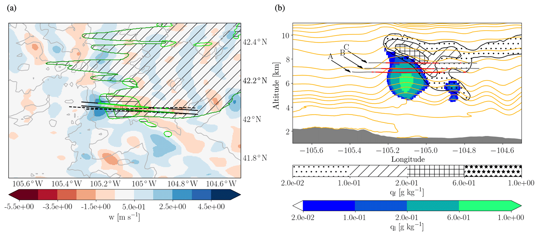
Figure 1(a) The modelled vertical velocity field at 7200 m, i.e. approximately the altitude of flight leg B, is shown by the colour shading (21:00 UTC). The dark blue (cyan) contour and horizontal (diagonal) hatching indicates where liquid (frozen) cloud water content in the model exceeds 0.02 g kg⁻¹. The colour shading in the area between the two grey straight lines shows the observed vertical velocity along flight leg B, and the blue (green) colouring of the grey lines indicate observed cloud liquid (ice) exceeding 0.02 g kg⁻¹. The black dashed lines show the location of the aircraft legs at 6900 and 6780 m. Black contours indicate the topography. (b) Vertical cross section through the wave cloud at 42.05^∘ N (21:00 UTC). The colour shading represents the modelled liquid water content; the contour lines with the hatching the modelled ice water content and the orange lines indicate isentropes. The horizontal lines show the projection of the flight path on the plane of the cross section, where red colouring of the lines indicates observed cloudy conditions (condensed water content larger than 10⁻⁷ kg kg⁻¹). The grey area at the bottom of the plot shows the topography.

Cloud microphysics are described by the CASIM module (Sect. 2.4) as in the UM simulations. As in the UM simulations, the sensitivity to the heterogeneous freezing parameterizations as well as assumptions for the CCN activation of INP is tested as detailed in Sect. 2.4. Together with the different settings for dynamic and thermodynamic conditions, we have a total of 45 360 two-dimensional, idealized simulations.

2.4 The CASIM module

The Cloud-AeroSol Interacting Microphysics (CASIM) module is a recently developed double-moment cloud microphysics scheme for the UM (Shipway and Hill, 2012; Hill et al., 2015; Stevens et al., 2018; Miltenberger et al., 2018). Hydrometeors are represented by five different species, the size distribution of which is assumed to be a generalized gamma distribution with a fixed width. Hydrometeor mass and number of each hydrometeor species are computed prognostically. CASIM also includes prognostic mass and number of three soluble and one insoluble aerosol modes, for which log-normal distribution with a fixed width are assumed. Additional tracers for aerosols incorporated into hydrometeors are available, which are transported in accordance with the hydrometeors, i.e. including sedimentation. The in-cloud aerosol tracers allow for an explicit representation of immersion freezing and to investigate the vertical transport of aerosol by hydrometeor sedimentation.

Key microphysical processes to be investigated in the mixed-phase clouds are activation of aerosols to cloud droplets, heterogeneous freezing, growth (sublimation) of ice crystals by vapour deposition, aggregation of ice crystals, and sedimentation of ice-phase hydrometeors. All of these processes are represented in the CASIM module. Activation of aerosol to cloud droplets is described with the parameterization of Abdul-Razzak and Ghan (2000). For the activation of the “insoluble” aerosol category we assume a soluble fraction on the dust particles, which is prescribed as 0.01 %, 0.1 %, and 99 % in three sets of sensitivity simulations. The chemical analysis of measured INP by Pratt et al. (2010) suggests that a substantial soluble fraction on INPs is realistic for the considered case. The activated INPs are then used to predict the ice crystal number concentration using parameterizations of immersion freezing from DeMott et al. (2010) (DM10), Niemand et al. (2012) (N12), Atkinson et al. (2013) (A13), Tobo et al. (2013) (T13), and DeMott et al. (2015) (DM15). For the A13 parameterization, we assume that 25 % of the dust surface is feldspar. Deposition and contact freezing are currently not represented in CASIM, but previous studies suggest these are not of major importance for mixed-phase orographic clouds. In addition, we have conducted simulations, in which the insoluble aerosol number concentration is directly used in these parameterizations irrespective of whether is was incorporated into liquid first. The latter is the standard approach in all models that do not track aerosol in hydrometeors. As the observed wave cloud reaches temperatures colder than −38 ^∘C homogeneous freezing is also important. Homogeneous freezing of cloud droplets is parameterized in CASIM following Jeffery and Austin (1997). In order to test the impact of homogeneous freezing on the simulated cloud microphysical structure and in particular the ice crystal number concentration, an additional simulation has been conducted, in which homogeneous freezing is switched off (“nohom”, heterogeneous freezing according to DM10). Thus in total, we have 21 sensitivity experiments with different representations of immersion freezing. For the sedimentation of ice-phase hydrometeors we use fixed diameter–fallspeed relations. For ice crystals the mass m_i is related to the mean particle diameter D_i via $m_i=\frac{\mathit{\pi }}{\mathrm{6}}\cdot \mathrm{200}$ kg m⁻³ $D_i^{\mathrm{3}}$. The fallspeed v_i is then computed according to v_i=71.34 m^0.3365 s⁻¹ $\cdot D_i^{\mathrm{0.6635}}({\mathit{\rho }}_{\mathrm{0}}{\mathit{\rho }}^{-\mathrm{1}}{)}^{\mathrm{0.5}}$, where ρ is the air density. The sedimentation fluxes will be sensitive to the parameters used in the mass–diameter and diameter–fallspeed relations, but we leave exploring this sensitivity to a future study.

2.5 Trajectory analysis

Kinematic air mass trajectories are computed to detect changes in specific humidity and aerosol number density due to sedimenting hydrometeors in the wave cloud. Trajectories are calculated with the Lagrangian Analysis Tool (Sprenger and Wernli, 2015), which has been adapted to UM output, from the resolved wind field at 5 min temporal resolution. For the KiD model, trajectories are calculated analytically based on the prescribed wind field (Eq. 1).

3.1 Thermodynamic conditions

The geometry of wave clouds is strongly controlled by the upstream humidity and temperature profile as well as the vertical velocity field.

Figure 2a shows a comparison of the upstream temperature profile. The air temperature in the model is slightly higher than observed at all vertical levels, if evaluated at the time and location of the aircraft observations, with a deviation of about 2 K for flight leg A and less than 0.1 K for flight leg C. The model suggests that the upstream temperature varied by up to 2.5 K during the time window of the observations, i.e. between 20:40 and 21:20 UTC.

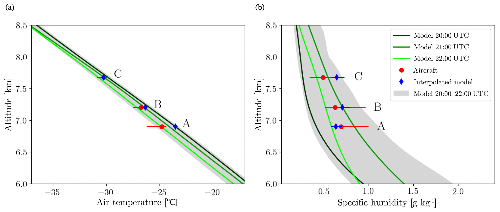
Figure 2Comparison of (a) upstream temperature and (b) specific humidity profiles from the UM simulation and aircraft data. Upstream conditions from aircraft data are computed from the non-cloudy sections of the aircraft legs west of −105^∘ E. Red circles indicate the mean value along these portions of the aircraft legs, and the bars indicate the variability. The model values are taken from the grid column closest to the average location of these upstream aircraft segments (green lines) at times between 20:00 and 21:00 UTC, i.e. bracketing the time of the observations between ∼ 20:40 and ∼ 21:20 UTC. The cyan shading shows the variability in temperature and specific humidity in this grid column for all output times between 20:00 and 22:00 UTC. The blue diamonds and bars show the model data interpolated to the flight track and evaluated in the same way as the aircraft data.

Download

The upstream specific humidity is compared in Fig. 2b. In general the model is somewhat more humid than observed at the time and location of flight leg C with a deviation of about 0.2 g kg⁻¹. The model also suggests a quite large variability in the upstream specific humidity (roughly by a factor of 2) in the time window of the observations with a gradual moistening before 21:00 UTC and a subsequent drying. As all observation data are within the modelled spread of specific humidity values, the agreement is fairly good. As the temporal evolution or zonal variation in the humidity profile is not well characterized by the observations, it is not straightforward to assess if and to what degree the differences between model and observed specific profiles impact the condensate content along the flight paths.

In Fig. 3 the observed vertical velocity along the three flight legs is compared to the modelled vertical velocity. While in the figure we also show the vertical velocity interpolated onto the flight path (dark blue), for the analysis we use hypothetical flight paths, which are parallel to the mean modelled streamline (grey lines). Hypothetical flight paths have a horizontal spacing of 250 m in zonal direction and run through the centre of the wave clouds, i.e. have a peak vertical velocity larger than 2.5 m s⁻¹. Using these hypothetical flight paths instead of the actual aircraft track eliminates the impact of slightly different horizontal wind direction in model simulations and the observed flow. The mean flow is from west to east, i.e. from left to right in these plots, and the cloud forms at the first peak in vertical velocity. The amplitude of the wave in terms of the vertical velocity is well captured in the model at all three altitudes with maximum deviations of less than 1 m s⁻¹. Note that the uncertainty in the vertical velocity observations can be up to several tenths of 1 m s⁻¹ (e.g. Field et al., 2012). The width of the positive vertical velocity peak is slightly larger in the model than in the observations, and the peak occurs slightly further east. The secondary peaks in vertical velocity downstream of the main wave are less well captured, particularly for flight leg C (Fig. 3a). For the cloud formation, the vertical displacement of air parcels is more important than the maximum vertical velocity. The vertical displacement depends on the amplitude, wavelength, and vertical structure of the wave. As vertical velocity observations are only available along the flight track, it is not possible to rigorously evaluate the modelled vertical displacement.

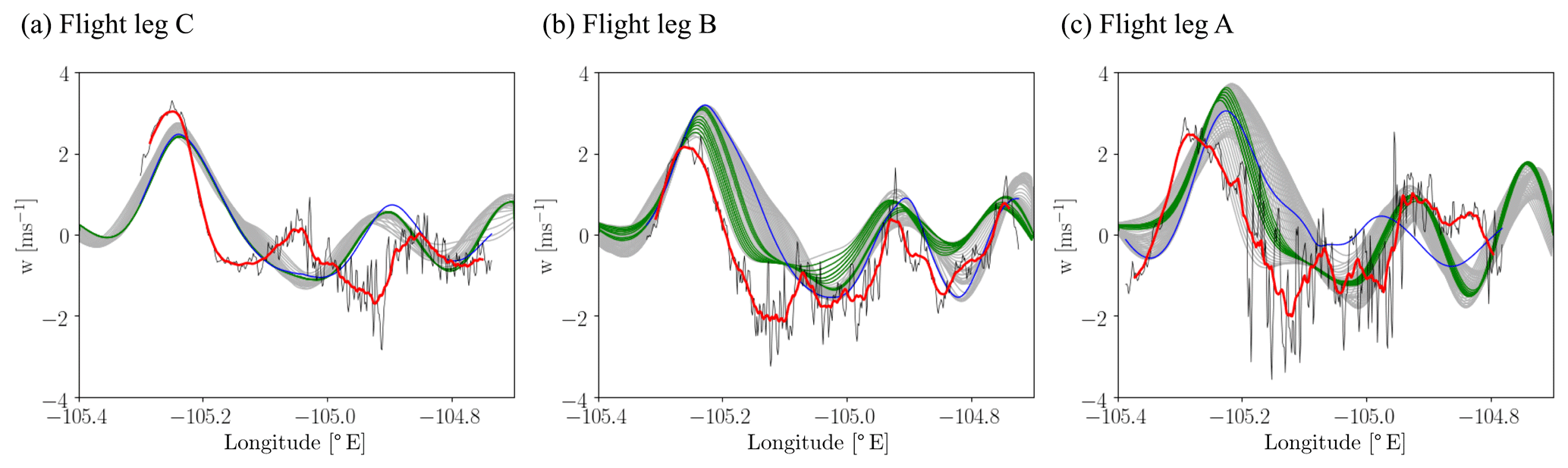
Figure 3Vertical velocity along (a) flight leg C (7680 m, 21:20 UTC), (b) flight leg B (7200 m, 21:00 UTC), and (c) flight leg A (6900 m, 20:40 UTC). The red solid line shows the aircraft data smoothed with a 20 s moving average filter (full 1 Hz data shown by the thin black line). The blue line shows the modelled aircraft velocity interpolated to the aircraft track. The grey lines show the vertical velocity along tangents to the mean streamline (including a deviation corresponding to the deviation between the observed mean horizontal wind direction and the direction of the aircraft track), for which the peak vertical velocity exceeds 2.5 m s⁻¹. This threshold was chosen to focus on the centre of the wave cloud only. The green line shows the tangent for which the Pearson correlation (including a lag of ±20 s) with the observed vertical velocity is larger than 0.95. To account for the temperature bias of the model, model data are taken 200 m above the altitude of the flight track.

Download

In summary, the modelled air temperature deviates less than 1 K from observations, the specific humidity less than 0.2 g kg⁻¹, and the vertical velocity less than 1 m s⁻¹. To our knowledge this is the first study, in which a direct comparison of aircraft measurements and simulations from a regional numerical weather prediction is done. There are many sources of uncertainty in regional numerical weather prediction models including uncertainty in the analysis used for initial and boundary conditions, the representation of orography, drag, dynamics, and microphysics. In addition, upstream conditions vary in time, which is not fully captured by the aircraft measurements. Given these issues, the agreement between modelled thermodynamic and dynamic conditions seems to be sufficiently good for an in-depth comparison of the cloud microphysical structure as well as investigations of the vertical fluxes of water vapour and aerosol. Due to the small temperature bias in the model, in the following we always compare the aircraft data with the model data 200 m above the altitude of the flight track. This eliminates the temperature bias (Fig. S1 in the Supplement) and allows for a better comparison of the ice nucleation.

3.2 Cloud structure

The microphysical data along the various aircraft legs allow for a detailed analysis of the microphysical processes due to the mainly laminar flow in the wave clouds, albeit not providing a truly Lagrangian perspective. Note that all flight legs are along or against the average wind direction, i.e. streamlines are crossed at least twice (see also Field et al., 2012). The in-cloud, updraught-dominated region of the flight legs is characterized by a relatively constant air temperature (variations <0.5 K) and specific humidity (variations <0.1 g kg⁻¹) (Figs. 4a–c, S1) in both the model and the observational data. The constant specific humidity reflects water saturated conditions given the observed constant in-cloud temperature. Consistent with the similar temperature in model and observation, the in-cloud specific humidity is very similar in both datasets. This is partly by design as the measured specific humidity was corrected such that the relative humidity is on average 100 % in regions with liquid water content larger than 0.02 g kg⁻¹ (Heymsfield et al., 2011).

Figure 4Comparison of (a–c) specific humidity and (d–f) total condensation mass mixing ratio for the three different flight legs. The flight legs are shown in the sequence of decreasing flight altitude from left to right. The thick black line shows the smoothed aircraft data (thin black line shows 1 Hz data). For the total water content (d–f) data from the CVI (thick solid black line) as well as the sum of King liquid water probe data and 2DS (2DC) data (black dashed (dotted) line) are shown. Model data are interpolated to the same tangents of the mean streamlines as used in Fig. 3. With the exception of the CVI data, the observed total water content includes only ice crystals larger than 50 µm. From the model results, the ice water content for ice crystals larger than 50 µm is computed by integrating over the respective part of the assumed size distribution in the model using the prognostic variables of ice number concentration, ice mass mixing ratio, and the fixed shape parameter. The modelled variability in the variable along all these hypothetical flight paths is shown by the grey shading, while the thick coloured lines show the median values for simulations. The different coloured lines represent the different ice nucleation schemes, and different line styles indicate different assumptions about the amount of soluble material in the dust particles (solid: all dust acting as INP).

Download

The deviations in the spatial distribution and amount of total condensate content between model and observations are larger than in all other variables considered so far (Fig. 4d–f). In the upstream, updraught-dominated cloud section, i.e. west of $\sim -\mathrm{105.1}$^∘ E, the total condensate amount is clearly larger than in the observations for flight legs A and C. For these flight legs total condensate data from the various available sensors agree well in this part of the cloud (deviations of maximum value less than 3 % and 20 %, respectively). For flight leg B, King liquid water probe measured about twice the amount of condensate as the CVI. The King liquid water probe data agree with the model data within 60 % (10 %, 100 %) for flight legs A (B, C) for the peak value. In most model runs as well as in the observational data there is little ice in this part of the cloud (Fig. 5), and hence the total condensate is controlled by the upstream humidity and the total lifting up to the considered point. Given the small deviations in upstream humidity between model and observations, the higher modelled total condensate values are likely due to the somewhat larger vertical velocities, which together with the similar horizontal wavelength result in larger vertical displacements of air parcels than in the observations (Fig. 3). Simulations using the A13 parameterization have an even higher total condensate amount. In these simulations glaciation occurs very early (Fig. 5), and hence the saturation pressure over ice is relevant for the equilibrium condensate amount and not the saturation pressure over water. In the cloudy region further downstream, i.e. downstream of $\sim -\mathrm{105.1}$^∘ E, observations indicate a large increase in condensate amount, despite the prevailing downdraft. Note observational data from various sensors diverge in this part of the cloud. In the model, there is a small increase in total condensate downstream of $\sim -\mathrm{105.1}$^∘ E most conspicuous for flight leg C (Fig. 4f). This increase is, however, smaller than in the observations, in particular for flight legs B and A. In the simulation without homogeneous freezing, the increase is absent, suggesting that the increase in condensate is due to homogeneously formed ice crystal being transported in the downdraft. It is likely that the increase observed is due to the same mechanism.

Figure 5As Fig. 4 but showing the frozen hydrometeor (a–c) mass mixing ratio and (d–f) ice crystal number concentration. The data (mass mixing ratios as well as number concentrations) incorporate only crystals larger than 50 µm.

Download

The the horizontal extent of the cloud, in which liquid hydrometeors are present, is similar in the observations and the model simulation, further supporting the above conclusion of a good representation of the thermodynamic structure of the wave cloud in the model simulations (Fig. S2). As discussed for the total condensate, the liquid water content is overestimated by the model most likely due to differences in the vertical displacement or upstream humidity of the air parcels. The cloud droplet number concentration deviates by less than 20 cm⁻³ between model and observations for all simulations except those using A13, for which cloud droplets are depleted due to very efficient heterogeneous freezing (Fig. S2).

The comparison of frozen hydrometeor mass mixing ratios shows that the modelled onset of significant cloud glaciation is roughly consistent with the observations along the flight legs B and C at $\sim -\mathrm{105.1}$^∘ E but occurs later on the flight leg A (model: $\sim -\mathrm{105.13}$^∘ E; observations: $\sim -\mathrm{105.18}$^∘ E; Fig. 5a–c). The steep increase in the mass mixing ratio on flight legs B and C (downstream of $\sim -\mathrm{105.1}$^∘ E) is associated with a rapid increase in ice number concentration in the model (Fig. 5d, e) and occurs in the downdraft region. While both the 2D-C and the 2D-S data agree quite well in terms of the ice crystal number concentrations (within factor 2), the estimated ice crystal mass diverges. The large increase in ice crystal mass and number in the downdraft region is likely due to the downward transport of ice crystals formed by homogeneous freezing by the descending air with a minor contribution of sedimentation. The importance of homogeneously formed ice in the downdraft region is supported by the divergence of ice crystal number concentrations in the simulations with and without homogeneous freezing (compare orange and blue line in Fig. 5d–f). In the observations ice mass and number concentration increase also in the downdraft region. However, the ice water content, at least in the 2D-C data, increases before the strong increase in ice crystal number concentration. In the model the steep increase in crystal number concentrations occurs earlier than in the observations. We hypothesis that the earlier increase in ice water content, which generally coincides with the start of the downdraft regions is due to larger displacements of air parcels in the model (somewhat larger vertical velocities, Fig. 3) and hence a stronger downward transport of homogeneously formed ice crystals. Alternatively, too early an onset of homogeneous freezing or too rapid a sedimentation of ice crystals could also lead to the observed differences between model and observation. Based on the available data, none of these options can be ruled out. The first ice crystals larger than 50 µm appear in approximately the same location as in the observations at all altitudes, however with much larger concentrations. This suggests too large a droplet mass in the freezing event consistent with the overestimation of liquid condensate. Maximum ice crystal concentrations for most simulations agree within a factor of 2 on flight legs A and B, while they are about a factor 10 larger on the flight leg C (Fig. 5d–f). However, if not only the maximum concentration is considered, modelled and observed ice crystal number concentration is within a factor of 2 only for the lowest flight level, with differences of almost an order of magnitude on the higher flight levels. As pointed out earlier, simulations using the A13 parameterization strongly overestimate the ice crystal number concentration inducing too early an onset of glaciation. Different assumptions about the CCN activation of dust particles (different line styles of the same colour in Fig. 5) have only a small impact on the modelled ice crystal mass and number concentrations, with the largest impact in simulations using the N12 parameterization and flight leg C. Even for simulations with N12 the resulting differences are much smaller than the difference to the observed time series, and it is not clear whether representing CCN activation of dust particles yields an improvement based on these. As expected the location, at which ice crystals first appear, is shifting slightly downstream in simulations with a smaller soluble fraction on the dust particles. The horizontal extent of the ice tail in the model is overestimated for all flight legs, except flight leg A (Fig. 5c, f). The longevity of ice crystal in the model is very likely related to the smaller average ice crystal mass, i.e. the ratio of ice crystal mass mixing ratio and number concentration, and the untuned parameters used to compute the mean fallspeed from the ice crystal diameter.

For the comparison of liquid and ice hydrometeor number concentrations and mass mixing ratios it is important to also consider limitations of the observational data. Most importantly, only data for ice crystals larger than 50 µm are used. This has been taken into account by estimating the number and mass of ice crystals larger than 50 µm from the modelled total mass and number concentrations using the prescribed distribution and shape parameter in CASIM. If small ice crystals were abundant in the wave clouds, this would improve the match of model and observations in the cloud region dominated by heterogeneously formed ice crystals but deteriorate it in the region dominated by homogeneously formed crystal. Another issue is that the 2D-C may detect large drizzle, which hence would be misclassified as ice, and the CDP measurements may include small ice particles (D'Alessandro et al., 2019). It is very unlikely for drizzle drops to be present in wave clouds due to the cold temperatures and the short time parcels reside in the cloud (<30 min), and hence no significant bias of the ice crystal number concentrations is expected. If some ice particles would be included in the CDP measurement, this would also only have a very limited impact on the comparison as ice number concentrations are about 3 orders of magnitude smaller than cloud droplet number concentrations.

In summary, observations and model simulations (except those using the A13 parameterization) agree on the overall microphysical structure of the cloud with ice particles and cloud droplets coexisting, a similar location for the appearance of first ice crystals and ice crystals from the homogeneous freezing zone affecting cloud properties in the downdraft region. Despite the overall good agreement in the structure of the wave cloud, modelled and observed total condensate amount as well as ice crystal number concentration deviate clearly. The former is most likely caused by an overestimation of parcel vertical displacement in the model, while the overestimation in initial ice crystal number is related to either the heterogeneous freezing parameterizations used or too large a diameter of the newly formed ice crystals. Assuming the same number of crystals being nucleated at a specific temperature, a large initial crystal mass results in a larger fraction of these ice crystals being detected early on, as their size more quickly exceed the detection limit of 50 µm. In the following section we investigate in more detail how different heterogeneous freezing parameterizations influence the spatial distribution of ice crystal number concentration.

3.3 Temperature dependency of heterogeneous ice formation

The main difference between the various heterogeneous freezing parameterizations is the temperature dependency of INPs and the prefactors specifying the INP fraction of dust particles, as illustrated in Fig. 6. While observing the impact of INP temperature dependence in most clouds is challenging due to impacts of sedimentation and strong vertical motion, the laminar flow and quasi-Lagrangian nature of aircraft observations in orographic clouds may facilitate observations of the signature of INP temperature dependence in ice crystal number concentrations. In order to test this hypothesis in the model we focus on the ice crystal number concentration in the updraught region of the cloud, i.e. west of −105.1^∘ E, which is not influenced by homogeneously nucleated ice crystals (compare orange and blue lines in Fig. 5d–f). This modelled ice crystal number concentration is compared with the ice crystal number concentration expected from the heterogeneous freezing parameterization based on the temperature and the upstream dust profile (compare coloured markers and lines in Fig. 6). In general these agree very well, suggesting that we can use observations of ice crystal number concentration from the updraught region of orographic wave clouds to constrain the temperature dependence of INP concentration. The observed ice crystal number concentrations from the 2D-C for the different flight legs are shown in the black boxplots in Fig. 6. These data suggest a very weak temperature dependency of heterogeneous freezing in the observed wave cloud, which is only consistent with the DM10 parameterization. All other parameterizations appear to have too strong a temperature dependence. However, the temporal evolution of the upstream dust concentrations has to be considered as this can result in shallower or steeper temperature apparent temperature dependence. As the upstream dust profile was not monitored continuously and is constructed from the upstream observations along the flight legs, only the potential impact of time-varying dust concentrations can be assessed. For this we use the minimum and maximum observed upstream dust concentrations, irrespective of the observed altitude, to derive the resulting impact on the expected ice crystal number concentration; the shaded area in Fig. 6 indicates the spread in expected number concentrations, while the dashed lines represent a scenario with continuously decreasing upstream dust concentrations. If the latter scenario is considered, the observations are consistent also with the T13 simulation. Reliable observational data of the ice crystal size distribution are only available for particles larger than 50 µm. Hence, the analysis here considers only the largest observed ice crystal number concentration in the updraught region. While this limits the impact of different mean droplet volumes during freezing and potential differences in depositional growth, it introduces additional uncertainty into the comparison.

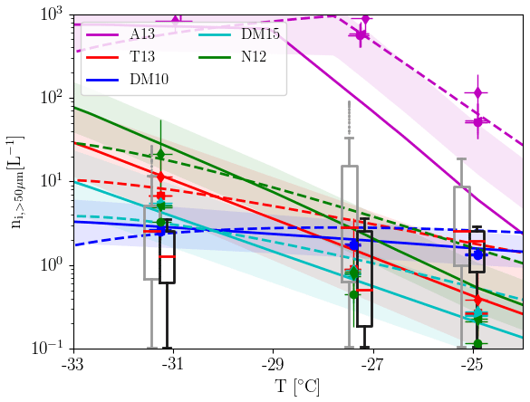
Figure 6Temperature dependency of ice crystal number concentration against air temperature from observations (2DC, boxplots) and UM model simulations (symbols; colours represent simulations with different ice nucleation schemes according to legend in Fig. 4a). Model data are interpolated to the hypothetical flight tracks and only considered in the first part of each flight leg, i.e. the updraught region. Observational data are also subsampled to include only data from the updraught region, which are shown in the black boxplots (grey boxplots show all data). The solid lines show the expected ice crystal number concentration based on ice nucleation only using the prescribed dust profiles. The colour shading illustrates the expected ice crystal number concentration for dust number concentrations within a factor of 2 of the used profile, i.e. compatible with range observed upstream of the cloud. Assuming a linear decrease in the upstream dust concentration over the time period of the observations together with the assenting flight pattern results in expected ice crystal number concentration as shown by the dashed lines.

Download

The comparison shows that all heterogeneous freezing parameterization, except that from Atkinson et al. (2013) are compatible with the observations within the anticipated uncertainty range. For simulations with the A13 parameterization we assume feldspar to be constitute 25 % of the dust surface, which is at the upper end of the composition of natural dust Atkinson et al. (2013). If a value closer to the lower bound of 1 % would have been used, A13 would be closer to the other parameterizations at −25 ^∘C but still predicts too high ice crystal concentrations at colder temperatures (Fig. S3). The experiment closest to the observations is DeMott et al. (2010), followed by DeMott et al. (2015) and Tobo et al. (2013) (compared black boxplots with dashed lines and shading in Fig. 6). However, it is unclear whether these parameterizations are most applicable in other cases or other geographic regions, as the INP activity is known to strongly depend on the chemical composition and size distribution of aerosols (e.g. Petters and Wright, 2015). Nevertheless, the presented results suggest that wave clouds can be used as natural laboratories to investigate the temperature dependence of heterogeneous freezing. To formulate constraints on the parameterizations, observations from more wave cloud events are necessary. In any future campaigns targeting orographic wave clouds, an emphasis should be placed on characterizing the full ice crystal size distribution as well as the temporal (and spatial) variation in the upstream aerosol concentration.

4.1 ICE-L case

One important impact of wave clouds on the evolution of the larger-scale atmospheric state is modification of water vapour and aerosol profiles through sedimentation of hydrometeors (in addition to the alteration of radiative fluxes). Vertical transport of water vapour and aerosols occurs in all clouds, but it is likely easier to observe these fluxes in wave clouds. The downward transport of water vapour depends strongly on the size and fall velocity of the formed hydrometeors. Thick warm-phase orographic clouds are known to produce significant precipitation. The downward water vapour transport is much smaller for mixed-phase wave clouds due to the smaller size and fallspeeds of ice crystals. However, according to the model simulations, the largest ice crystal diameters are on the order of 400–600 µm (not shown), which results in vertical displacement of about 700 m due to sedimentation over the roughly 30 min air parcels spend inside the cloud. Here, we quantify the downward transport of water and aerosol by considering the change in total water or aerosol number concentrations along trajectories through the wave cloud, Δq_t(z₀). We refer to the vertically integrated increase in total water in the lower part of the profile (equal to the decrease in total water in the upper part of the profile) as the total downward moisture transport (Δq_t). Fig. 7a and b show the Lagrangian change in total water along backwards trajectories starting in the lee of the cloud for simulations with the A13 and DM10 heterogeneous freezing parameterizations. In the time period after 80 min a typical sedimentation signal is obtained, with a depletion of the total water content in parcels above about 7 km and an increase in parcels below. At earlier times, this pattern is repeated twice in the vertical, and a closer inspection reveals that there are two cloudy layers in the UM simulations, one formed by homogeneous nucleation and the lower one by heterogeneous freezing. To assess the differences between simulations with different heterogeneous freezing, average profiles for the two time periods from all simulations are shown in Fig. 7c and d. The shading indicates the variability resulting from different starting latitudes of the trajectories. The mean profiles for simulations with all parameterizations except A13 are very similar and much smaller than the temporal variability. The larger INP concentrations predicted by A13 lead to much larger change in total water content Δq_t(z₀) particularly in the first part of the considered time period. The assumptions about the CCN activation of dust lead to very small differences in Δq_t(z₀) (Fig. S4a, b).

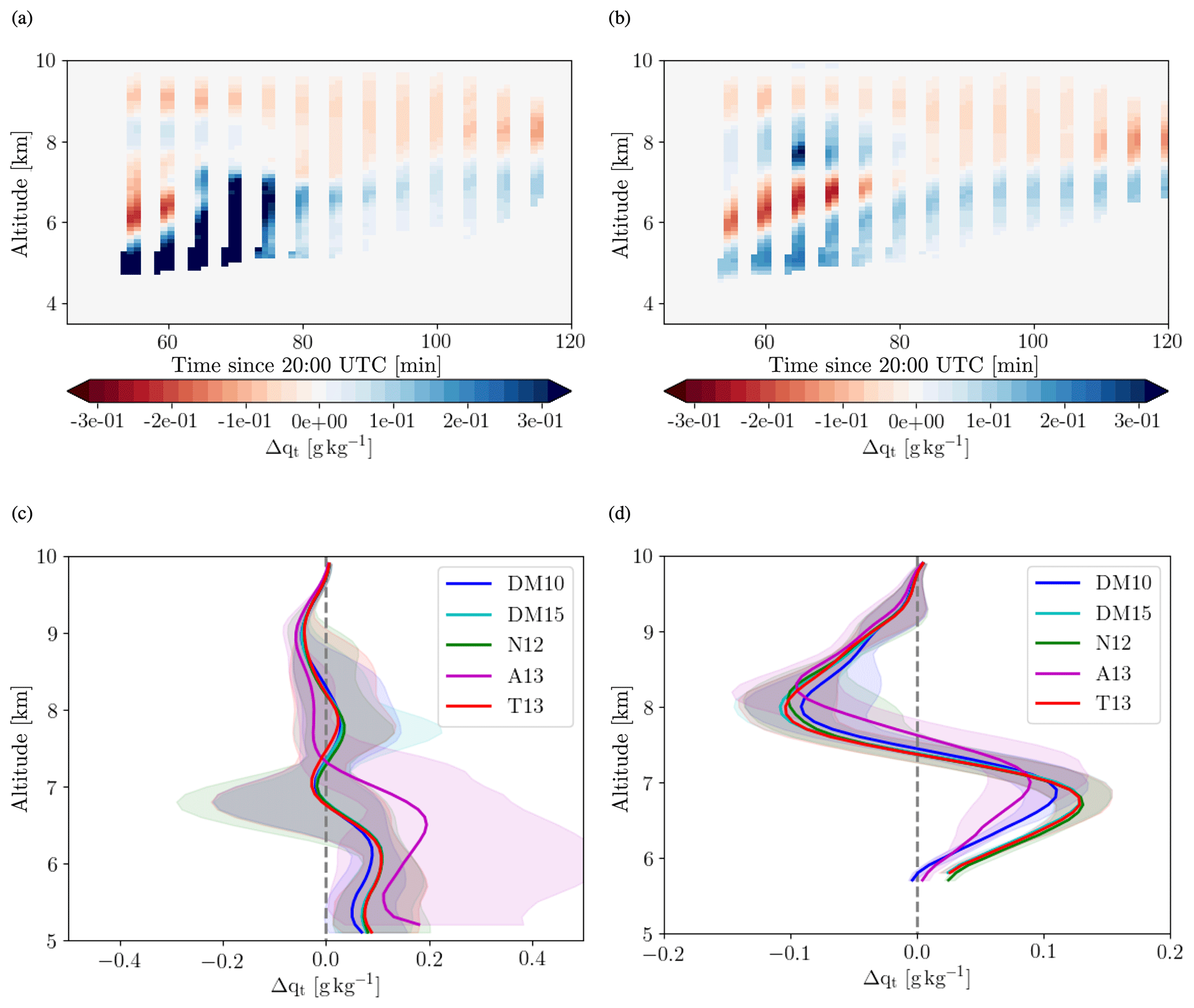
Figure 7(a, b) Difference in total water mass mixing ratio Δq_t between −105.35^∘ E (upstream) and −104.78^∘ E (downstream) along backward trajectories for simulations using the (a) A13 and the (b) DM10 ice nucleation parameterization. The differences are calculated as downstream values minus upstream values. The plot shows values at 42.1^∘ N, i.e. downstream of the centre of the wave cloud. The times on the abscissa indicate the arrival time of the trajectories at the downstream location. (c, d) Mean profiles of Δq_t for all simulations averaged between (c) 21:10 and 21:30 and (d) 21:40 and 22:00 UTC. The different colours correspond to simulations with different ice nucleation parameterizations, while the shading represents the temporal variability in the profiles. Note the travel time of the trajectories between the upstream and the downstream location is about 30 and 40 min.

Download

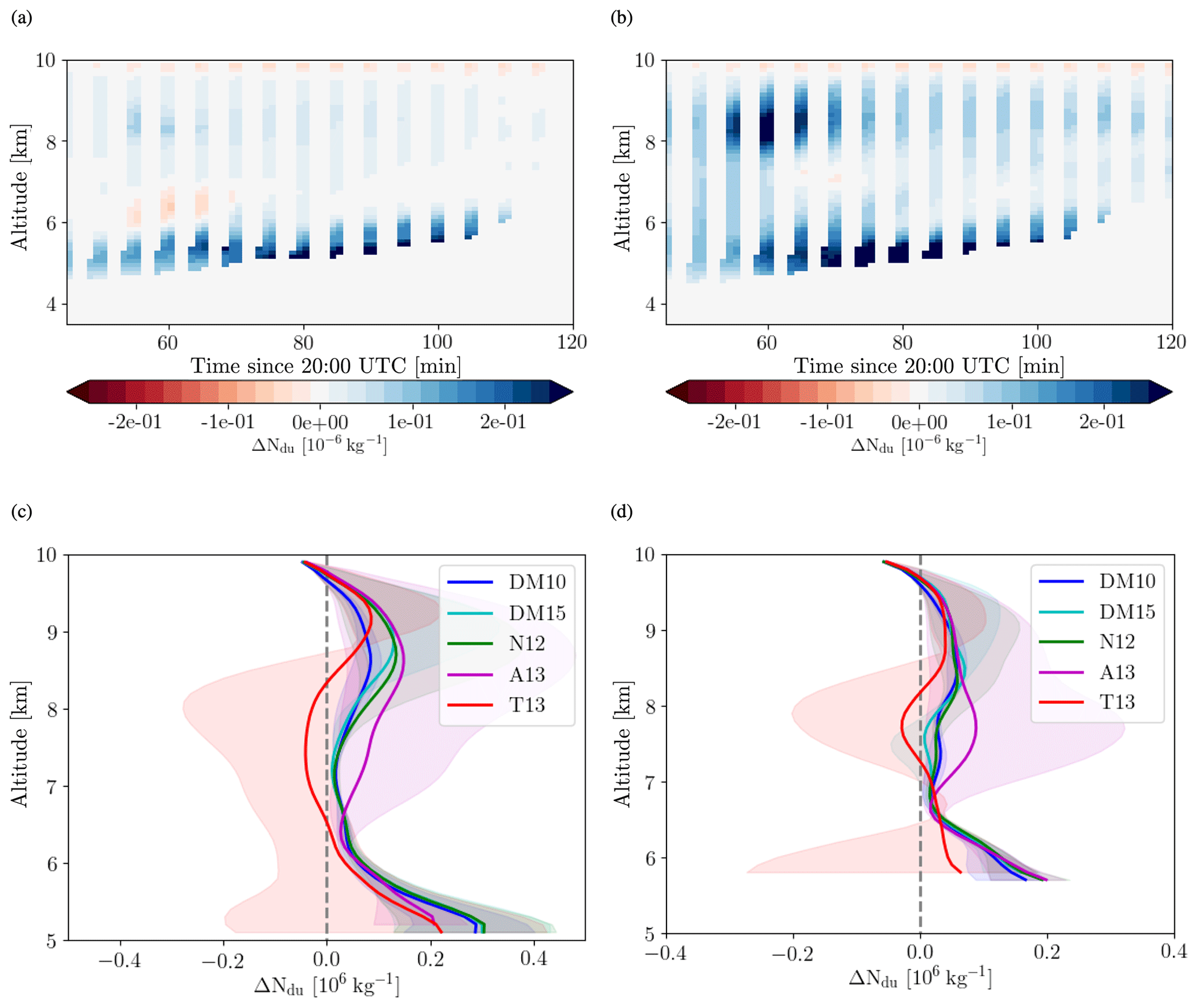
The CASIM microphysics explicitly considers the vertical transport of dust particles by hydrometeor sedimentation and therefore allows us to quantify the downward transport of aerosol by the wave cloud. The Lagrangian change in aerosol content is shown in Fig. 8. The vertical structure is different to Δq_t(z₀), with aerosol depletion only occurring at the very top of the cloud (above ∼9.7 km) and increases in aerosol number concentrations mainly towards cloud base. The modifications of the dust profiles are more sensitive to changes in the heterogeneous freezing parameterization than those of the total water content, with larger changes also in the shape of the profiles. However, the differences are again smaller than the temporal variability. The treatment of the CCN activation of dust (using all dust for heterogeneous freezing or presenting activation assuming some soluble fraction on dust particles) has a much larger impact on the vertical aerosol transport than on the moisture transport. The resulting differences in the profile are on the same order of magnitude as the temporal variability (Fig. S4c, d).

Figure 8As Fig. 7 but showing the change in dust number concentration.

Download

It would be interesting to constrain the downward transport with observational data, in particular given the uncertainties surrounding diameter–fallspeed relations often used in bulk models. The maximum change in q_t of about 0.1 g kg⁻¹ is, however, smaller than the temporal variation in the specific humidity (Fig. 2) during the average time a parcel needs to transit through the wave cloud (i.e. ∼30 min). As the aircraft data do not provide information on the temporal evolution of upstream humidity, it is not possible to use the aircraft data to constrain the vertical moisture transport by sedimentation. In addition, for such an assessment the construction of air parcel trajectories from the observed velocity field would be required. While this is in principle possible (e.g. Field et al., 2012), for the assessment of downward moisture transport, the error in the upstream positions of air parcels would need to be smaller than 500 m owing to the vertical gradient of upstream specific humidity. This is not feasible given the sparse observations of velocity (only sampled along flight legs) and the uncertainty in measured vertical velocity. However, detailed observations of the 3D velocity field for example with an on-board lidar system and a better characterization of the upstream and downstream humidity profiles, e.g. sampling in a quasi-Lagrangian manner, there is a potential for future field campaigns to constrain vertical transport of moisture by sedimenting hydrometeors from wave clouds.

Because wave clouds offer such an opportunity to detect sedimentation mediated vertical transport of moisture and aerosol we assess in the following section how its amplitude depends on the upstream thermodynamic conditions, which determine the cloud thickness and cloud top temperature, and on the horizontal wavelength of the gravity wave, which controls the horizontal extent of the cloud.

4.2 Downward moisture transport by sedimentation in idealized simulations

The modification of moisture and aerosol profiles by hydrometeor sedimentation is investigated for the ICE-L case study in the previous section. However, the cloud-integrated sedimentation fluxes will vary for different wavelength, cloud top temperatures, and cloud thicknesses and so will their impact on the vertical profiles of aerosol and moisture. To assess these dependencies, we use two-dimensional, idealized simulations with the KiD model (Sect. 2.3). Using an idealized model for this assessment allows us to vary the wavelength of the gravity wave, which would require changing the topography in the Unified Model. In addition, we can carry out a large number of simulations sampling a large proportion of the relevant phase space, which would not be possible with the UM due to the much larger computational costs. But we are able to link back to the case study by including the observed case in the phase space explored. Two exemplary realizations of wave cloud in the KiD model are shown in Fig. 9 along with the profiles of Lagrangian changes in moisture (Δ_Lagrq_t) and aerosol Δ_Lagrm_du. As in the UM simulations, the profiles of moisture and aerosol changes have distinctly different shapes: while aerosol changes are concentrated at cloud top and cloud base, moisture changes occurring throughout the cloud with peak values in the upper and lower half of the cloud, respectively.

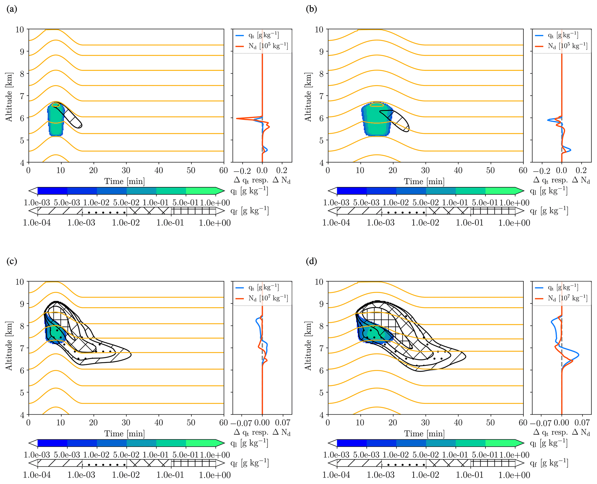
Figure 9Wave clouds in the KiD model. Simulations of waves with periods of (a, c) 1000 s and (b, d) 1800 s are shown. The cloud top temperature is −24 ^∘C in (a) and (b) and −50 ^∘C in (c) and (d). The cloud droplet mass mixing ratio is indicated by the colour shading, ice and snow mass mixing ratio by the hatched contours, and the isentropes by orange isolines with a spacing of 2 K. The small subpanels show the difference in total water content (light blue line) and the dust number concentration (red line) between the upstream and downstream. Note the different units for the dust number concentration change in (a) and (b) and (c) and (d), respectively.

Download

To explore the variation in the downward transport as a function of cloud geometry, we focus on the cloud-scale downward moisture (aerosol) transport Δq_t (Δm_du), which we define as the integral of positive Δ_Lagrq_t (Δ_Lagrm_du). Note that the integral over negative Δ_Lagrq_t (Δ_Lagrm_du) gives the same results due to mass conservation, albeit of course with a different sign (not shown). For further analysis we split the sedimentation flux into sedimentation of liquid (Δ_Lagrq_t,l) and frozen hydrometeors (Δ_Lagrq_t,l), which display a different dependence on the explored phase-space control parameters. Figure 10a summaries Δq_t,f for all investigated wave periods (abscissa) and cloud top temperatures (ordinate) for a cloud depth of 2000 m. Figure S5a is the equivalent for Δ_Lagrq_t,l. Δ_Lagrq_t,l is only important for cloud top temperatures warmer than $\sim -\mathrm{30}$ ^∘C (Fig. S5b). In both the UM and the KiD model rain formation is included as is the sedimentation of cloud droplets and rain drops. Rain formation is found in all simulations to be negligible, with the rain mass mixing ratio at least 1 order of magnitude smaller than the mass mixing ratio of any other hydrometeor. This is due to the short in-cloud residence timescales (<30 min), which according to the timescale analysis in Stevens and Seifert (2008) and Miltenberger et al. (2015) is too short for significant rain formation. As the dependence of Δ_Lagrq_t,l is quite different from Δ_Lagrq_t,f, and considerations of Δ_Lagrq_t,l are already published in Miltenberger et al. (2015), the following analysis will predominantly focus on Δ_Lagrq_t,f. Δ_Lagrq_t,f has also been computed from the UM simulations and is shown by the colour-filled circle at T=1800 s and $t_{\mathrm{ct}}=-\mathrm{45}$ ^∘C, which corresponds to the average cloud top temperature and residence time of parcels in the orographic cloud for the ICE-L case. In the UM only the central section of the wave cloud with largest vertical velocities is considered. Δq_t,f for the three-dimensional UM simulation and the idealized KiD simulation are comparable in value. This justifies the use of the KiD model to explore the dependence of Δq_t,f on the upstream thermodynamic profile and the wave period.

Figure 10Modification of (a, b) water and (c, d) dust profiles across wave clouds with vertical extent z_c of 2 km and various cloud top temperatures (ordinate) as well as periods (abscissa). Panels (a) and (c) show the mean value across KiD simulations with different ice nucleation and soluble fraction descriptions. Panels (b) and (d) show the variability resulting from varying the ice nucleation representation and the soluble fraction assumption, i.e. $({\mathrm{\Delta }}_{\mathrm{Lagr}}{q}_{\mathrm{t}}{\mathrm{|}}_{max}-{\mathrm{\Delta }}_{\mathrm{Lagr}}{q}_{\mathrm{t}}{\mathrm{|}}_{max})/{\mathrm{\Delta }}_{\mathrm{Lagr}}{q}_{\mathrm{t}}{\mathrm{|}}_{\mathrm{mean}}$. The colour-filled circles indicate the location of the ICE-L case study in the phase space. The colour of the circle shows the value obtained from the UM simulations of the ICE-L cloud.

Download

The most prominent feature in the variation in Δq_t,f over the sampled part of the phase space is the strong increase in Δ_Lagrq_t,f at about a cloud top temperature of −37 ^∘C, which is due to the onset of homogeneous freezing and hence a large increase in the frozen water content available for sedimentation. For all cloud top temperatures Δ_Lagrq_t,f increases towards longer wave periods as expected. These general patterns are consistent for all cloud thicknesses investigated (not shown). The downward moisture transport increase with larger cloud thickness, but the impact of cloud thickness is smaller than that of wave time period and cloud top temperature (not shown). Hence, the discussion in the following focusses on a single cloud thickness, although all sensitivity experiments are included in the formulation of the conceptual model. Consistent with the UM simulations, the parameterization used for heterogeneous freezing impacts the downward moisture transport. Fig. 10b shows the maximum difference between any two simulations with the same wave period, cloud top temperature, and cloud thickness but different heterogeneous freezing parameterizations (20 simulations for each combination of wave period, cloud top temperature, and cloud thickness). For the UM simulation the variability is about a factor of 5 larger (colour-filled circle in Fig. 10b), which is mainly due to the low values for the simulation with DM10 and ϵ=0.01. The impact of the parameterization choice is largest for cloud top temperatures just below the onset of homogeneous freezing (see e.g. Fig. 6). In this part of the parameter space Δ_Lagrq_t varies by up to a factor 10 between simulations with different heterogeneous freezing parameterizations. Differences between simulations with different heterogeneous freezing parameterizations are largest for wave periods larger than 800 s and cloud top temperatures between $\sim -\mathrm{30}$ and $\sim -\mathrm{38}$ ^∘C.

The downward transport of aerosol Δ_Lagrm_du is summarized in Fig. 10c and d. Δ_Lagrm_du and its variation with cloud microphysical parameterization choices are again very similar to the values obtained from the UM simulation (colour-filled circles in Fig. 10c, d). The aerosol downward transport increases, similar to the downward moisture transport, with longer wave periods and towards colder cloud top temperatures. The increase with decreasing cloud top temperature is, however, smoother than for Δ_Lagrq_t. Towards the onset of homogeneous freezing most heterogeneous freezing parameterizations predict that a substantial fraction of dust is activated as INP, and hence there is no step change at the onset of homogeneous freezing. Differences between simulations with different settings in the cloud microphysics are largest for wave periods larger than 600 s and cloud top temperatures between $\sim -\mathrm{19}$ and $\sim -\mathrm{28}$ ^∘C.

A conceptual model of the moisture transport by sedimenting frozen hydrometeors provides insight into the key variables controlling the modification of the moisture profile and may be used to represent these in models with a lower spatial resolution. Similar to previously proposed conceptional models for orographic precipitation (Smith, 1979; Smith and Barstad, 2004; Seifert and Zängl, 2010; Miltenberger et al., 2015), we chose an ansatz based on the consideration of the characteristic timescales of the cloud:

The first term on the right side of the equation describes how much water is transferred from the gas-phase to frozen condensate due to depositional growth and freezing, while the second term describes the sedimentation of the condensate. The key variables are (i) the potential condensate G_pot, which is the maximum cloud condensate possible given thermodynamic constraints, initial humidity, and vertical displacement; (ii) the in-cloud residence time τ_ic, i.e. the time available for cloud microphysical processes; (iii) the timescale for depositional growth of ice hydrometeors τ_dep; and (iv) the timescale for sedimentation τ_sedi. Note that in contrast to parcel-oriented formulations these timescales refer to the entire cloud and not to individual air parcels. Finally, G_nuc denotes the condensate formed during ice crystal nucleation via homogeneous or heterogeneous freezing. A similar approach has been suggested by Seifert and Zängl (2010) and Miltenberger et al. (2015) for describing the precipitation formation in warm-phase orographic clouds. As we show in the following, all parameters in Eq. (3) can be estimated from the upstream thermodynamic profiles and expected vertical displacement.

As mentioned above, we focus here on the sedimentation flux of frozen hydrometeors. For cloud top temperatures warmer than about $\sim -\mathrm{30}$ ^∘C, the impact of cloud droplet sedimentation is comparable to or larger than that of frozen hydrometeor sedimentation (Fig. S5b). In contrast to Δ_Lagrq_t,f, Δ_Lagrq_t,l depends in our set of experiments only on τ_ic. The main reason for this is that a saturation adjustment scheme is used in the UM and KiD model, and only a specific maximum vertical displacement is considered (see Sect. 2.3). Hence, for the following ansatz is chosen for moisture transport by sedimenting cloud droplets:

The potential liquid condensate G_pot,l, i.e. the difference between the upstream specific humidity and the saturation water content over water at the coldest point along the trajectory, and tau_ic,l can be estimated using the same procedure as outlined below for G_pot and τ_ic by considering the saturation mass mixing ratio over water instead of that over ice. The sedimentation timescale τ_sedi,l can be estimated by using the profile of G_pot,l(z₀) together with the typical cloud droplet number concentration (here 70 cm⁻³), the fallspeed–diameter and mass–diameter relationships used in the model, and the cloud depth. Note that despite being significant compared to the frozen hydrometeor sedimentation flux, fluxes are generally very small for temperatures warmer than −30 ^∘C. In the following, we discuss in detail the estimates for variables in Eq. (3), in line with the focus of the paper.

The potential condensate is the maximum condensate amount that would occur along a wave cloud trajectory if the air parcel's ice water content were in thermodynamic equilibrium, i.e. roughly the difference between the upstream vapour content and the saturation water content over ice at the coldest point along the trajectory. In warm-phase clouds the condensate amount in absence of sedimentation is often close to the potential condensate as a result of fairly small vapour deposition timescales (∼1 s), as e.g. used in saturation adjustment parameterizations. However, in mixed- and ice-phase clouds the potential condensate is typically not realized due to the longer timescales for depositional growth (on the order of 1000 s). G_pot is not used as a measure of the condensate formed in the cloud but as a “virtual” reservoir species from which condensate can be formed. Along air parcel trajectories G_pot can be directly computed as the difference between the upstream specific humidity and the saturation pressure over ice at the coldest point along the trajectory, if latent heating from phase changes of water are neglected. Using trajectory data from the KiD experiments, the variation in G_pot,Lagr with the wave period and cloud top temperature can be quantified (Fig. 11a). Further G_pot can be computed from the wave amplitude A and the upstream temperature t₀, specific humidity q_v,0, and pressure p₀ profiles by assuming dry-adiabatic ascent of the parcel (lapse rate γ) and a hydrostatic balanced atmosphere as follows:

Integrating above equation over all altitudes where $q_{v,\mathrm{0}}>q_{i,\mathrm{sat}}(t_{\mathrm{0}}+A\mathit{\gamma })$ gives an estimate of G_pot, which for our KiD simulations deviates less than 5 % from the Lagrangian estimate shown in Fig. 11a (Fig. S6a).

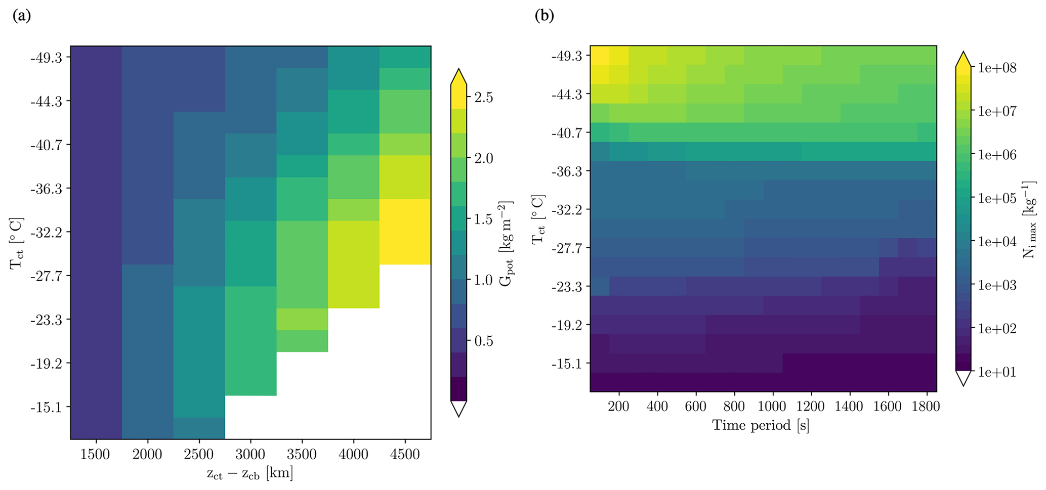
Figure 11(a) Potential condensate G_pot as a function of cloud thickness and cloud top temperature. (b) Maximum ice crystal number concentration $n_{\mathrm{i},max,\mathrm{Lagr}}$ as a function of wave period and cloud top temperature for clouds with a thickness of 2 km. $n_{\mathrm{i},max,\mathrm{Lagr}}$ is the maximum integrated ice crystal formation rate, including homogeneous and heterogeneous freezing, along any trajectory through the wave cloud.

Download

Another important cloud microphysical variable that will be required for parameterizing the characteristic timescales is the number of ice crystals in each cloud. To characterize the variability across the different clouds, we use only the maximum possible number of ice crystals $n_{\mathrm{i},max}$ formed by either homogeneous or heterogeneous freezing. In the Lagrangian data, this is the integral of homogeneous and heterogeneous nucleation rates along the trajectory passing just below cloud top. Figure 11b shows that $n_{\mathrm{i},max,\mathrm{Lagr}}$ depends strongly on cloud top temperature with a major increase around $t_{\mathrm{ct}}\approx -\mathrm{38}$ ^∘C reflecting the transition to clouds dominated by homogeneous freezing. For clouds with colder cloud tops there is also a clear dependence on the time period of the wave clouds, reflecting the interaction between the nucleation and growth of newly formed ice crystals (e.g. Kärcher et al., 2006). For the conceptual model, we find that using the heterogeneous parameterization used in the KiD model together with the minimum temperature expected from the maximum vertical displacement gives a reasonable estimate for temperatures warmer than −38 ^∘C. For colder cloud top temperatures, we use the homogeneous nucleation rate from the DM10 parameterization (consistent with CASIM microphysics) and a correction factor depending on the wave period: $\mathrm{0.932}\cdot {\log }_{\mathrm{10}}\left(T\right)+\mathrm{0.228}$ for $t_{\mathrm{ct}}<-\mathrm{42.5}$ ^∘C and $\mathrm{1.48}\cdot {\log }_{\mathrm{10}}\left(T\right)-\mathrm{1.48}$ for $t_{\mathrm{ct}}>-\mathrm{42.5}$ ^∘C. Closely related to the ice crystal number is also the term G_nuc describing the ice crystal mass formed by homogeneous or heterogeneous freezing. G_nuc can be estimated from $n_{\mathrm{i},max}$ and a typical particle mass $\stackrel{\mathrm{‾}}{q_i}$, which can be directly obtain from the KiD simulations: $\stackrel{\mathrm{‾}}{q_i}={\mathrm{10}}^{-\mathrm{11.5}}$ kg kg⁻¹ (10^−9.6 kg kg⁻¹) for clouds dominated by homogeneous (heterogeneous) freezing.

The in-cloud residence time τ_ic describes the time available for condensate and precipitation formation (e.g. for warm clouds; Miltenberger et al., 2015). Here, we define τ_ic as time during which air parcels are supersaturated with respect to ice. This timescale τ_ic,Lagr can be directly quantified from the KiD-model air mass trajectories (Fig. 12a) or analytically calculated from the prescribed wave flow and the upstream humidity profile:

with η_i,sat the vertical displacement required to reach ice saturation. The deviations between this estimate and the Lagrangian metric are less than 5 % (Fig. S6b). From the resulting vertical profile of τ_ic the largest timescale is selected (only considering cloudy parcels).

Figure 12Lagrangian estimates of (a) the in-cloud residence timescale τ_ic, (b) the deposition timescale τ_dep, and (c) the sedimentation timescale τ_sedi. Results are shown for simulations with a cloud thickness of 2 km.

Download

The depositional timescale τ_dep describes the characteristic timescale for the reduction of ice supersaturation for w=0 m s⁻¹ and an ice crystal population characterized by the number concentration n_i and mean ice particle diameter d_i. The concept of describing depositional growth of ice crystals with a characteristic timescale τ_dep is frequently used in literature and cloud microphysical parameterizations (e.g. Khvorostyanov, 1995): ${\mathit{\tau }}_{\mathrm{dep}}=(g{n}_{\mathrm{i}}{d}_{\mathrm{i}}{c}_{\mathrm{i}}f{)}^{-\mathrm{1}}$, where $g=\mathrm{4}\mathit{\pi }\cdot \left(L_{\mathrm{ed}}^{\mathrm{2}}\right(K_t{R}_{\mathrm{d}}{t}^{\mathrm{2}}{)}^{-\mathrm{1}}+R_{\mathrm{d}}t(D_{\mathrm{vtp}}{e}_{\mathrm{s},\mathrm{i}}{)}^{-\mathrm{1}}{)}^{-\mathrm{1}}$, L_ed is the latent heat of sublimation, K_t is the heat conductivity, R_d is the specific gas constant for dry air, D_vtp is the diffusivity of water vapour, e_s,i is the saturation vapour pressure over ice, c_i is the capacitance of the ice crystals, and f is a ventilation factor. This concept needs to be extended to a single characteristic timescale for the entire cloud. To estimate this timescale we again utilize the KiD simulations. The cloud-scale deposition timescale can be estimated from the integrated deposition D and freezing rates G_nuc as well as τ_ic according to ${\mathit{\tau }}_{\mathrm{dep},\mathrm{Lagr}}={\mathit{\tau }}_{\mathrm{ic},\mathrm{Lagr}}{\left(\log (\mathrm{1}-D(G_{\mathrm{pot}}-G_{\mathrm{nuc}}{)}^{-\mathrm{1}}\right)}^{-\mathrm{1}}$. The resulting estimates are shown in Fig. 12b. Immediately obvious is an inverse relation to the ice crystal number concentration, as expected from air parcel considerations, but this is not the sole determinant. In order to estimate τ_dep from the a priori known parameters, i.e. upstream profiles and vertical displacement, we determined the following least-square fits to the KiD model data (Fig. S6c):

The subdivision is necessary due to the fundamentally different behaviour in the parts of the parameter space dominated by homogeneous and heterogeneous freezing.

Finally, the sedimentation timescale needs to be determined, for which we use the same approach as for the deposition timescale, i.e. diagnosing a cloud-wide timescale from the KiD model and constructing a statistical model. The timescale is estimated from the KiD model according to ${\mathit{\tau }}_{\mathrm{sedi},L}={\mathit{\tau }}_{\mathrm{ic},L}{\left(\log (\mathrm{1}-\mathrm{\Delta }{q}_{\mathrm{sedi}}(D+G_{\mathrm{nuc}}{)}^{-\mathrm{1}}\right)}^{-\mathrm{1}}$. The results are shown in Fig. 12c. The sedimentation velocity in the KiD model is described using a prescribed diameter–fallspeed relation. Consistently, the τ_sedi increases for clouds with larger n_i. In addition to this information, we find that it is necessary to incorporate information on the time period and cloud thickness in the statistical model likely due to their impact on the cloud microphysical evolution (Fig. S6d):

By using Eqs. (3) to (8) with the described approximation of n_i,max, the total downward moisture transport by sedimentation can be computed based on the upstream dust concentration, the upstream profiles of temperature, humidity, and pressure, and the maximum vertical displacement. The parameterized Δq_t is shown in Fig. 13a. Comparing this figure with the results from the full KiD model (Fig. 10a) shows very similar dependencies on wave period and cloud top temperature. Note that Fig. 10a shows the average Δq_t from simulations with different heterogeneous freezing parameterizations, while Fig. 13a shows data only for simulations with DM10 – hence the differences in absolute values. The absolute values from the conceptual model agree well with the simulations from the full KiD model with discrepancies mostly smaller than 30 % (Fig. 13b, Fig. S7).

Figure 13(a) Total downward transport of water predicted using Eqs. (3) to (8) across wave clouds with vertical extent z_c of 2 m, the DM10 heterogeneous freezing parameterization, and various cloud top temperatures (ordinate) as well as periods (abscissa). (b) Normalized difference between Δq_t predicted by the conceptual model and the full KiD model for different cloud top temperatures. The data shown in (b) include the full simulations set with all cloud top temperature, wavelength, and cloud thickness specified in Sect. 2.3.

Download