the Creative Commons Attribution 4.0 License.
the Creative Commons Attribution 4.0 License.
 | 23 Jan 2020
Ice supersaturated regions: properties and validation of ERA-Interim reanalysis with IAGOS in situ water vapour measurements
Patrick Neis
Susanne Rohs
Bastien Sauvage
Cirrus clouds and their potential formation regions, so-called ice supersaturated regions (ISSRs), with values of relative humidity with respect to ice exceeding 100 %, occur frequently in the tropopause region. It is assumed that ISSRs and cirrus clouds can change the tropopause structure by diabatic processes, driven by latent heating due to phase transition and interaction with radiation. For many research questions, a three-dimensional picture including a sufficient temporal resolution of the water vapour fields in the tropopause region is required. This requirement is fulfilled nowadays by reanalysis products such as the European Centre for Medium-Range Weather Forecasts (ECMWF) ERA-Interim reanalysis. However, for a meaningful investigation of water vapour in the tropopause region, a comparison of the reanalysis data with measurement is advisable, since it is difficult to measure water vapour and to assimilate meaningful measurements into reanalysis products. Here, we present an intercomparison of high-resolution in situ measurements aboard passenger aircraft within the European Research Infrastructure IAGOS (In-service Aircraft for a Global Observing System; http://www.iagos.org, last access: 15 January 2020) with ERA-Interim. Temperature and humidity data over the North Atlantic from 2000 to 2009 are compared relative to the dynamical tropopause. The comparison of the temperature shows good agreement between the measurement and ERA-Interim. While ERA-Interim also shows the main features of the water vapour measurements of IAGOS, the variability of the data is clearly smaller in the reanalysis data set. The combination of temperature and water vapour leads to the relative humidity with respect to ice (RHi). Here, ERA-Interim deviates from the measurements concerning values larger than RHi=100 %, both in number and strength of supersaturation. Also, pathlengths of ISSRs along flight tracks are investigated, representing macrophysical properties as linked to atmospheric flows. The comparison of ISSR pathlengths shows distinct differences, which can be traced back to the spatial resolution of both data sets. Also, the seasonal cycle and height dependence of pathlengths changes for the different data sets due to their spatial resolution. IAGOS shows a significantly greater amount of smaller ISSRs compared to ERA-Interim. Good agreement begins only at pathlengths on the order of the ERA-Interim spatial resolution and larger.


Water vapour is the most important greenhouse gas in the atmosphere and therefore plays a major role in the Earth's radiative balance (Myhre et al., 2013). Especially in condensed form, water is also of large significance for planetary radiation. Clouds can reflect incoming solar radiation while absorbing and re-emitting longwave radiation from the Earth. Particularly the effect of cirrus clouds is still challenging. Whether a cirrus cloud has a net warming or cooling effect on the Earth's atmosphere depends strongly on altitude, available humidity and microphysical properties like number, size and type of ice nuclei (IN). Even the same exact cirrus cloud can change the sign of its net forcing depending on the time of day (Joos et al., 2014). Besides natural cirrus clouds, also the aircraft-induced contrail cirrus clouds play an important role for the radiative budget (Kärcher, 2018).
The control parameter for cold cloud formation in the upper troposphere is relative humidity with respect to ice, which reaches supersaturation by exceeding the temperature-dependent water-holding capacity of the air mass (Gierens and Spichtinger, 2000; Spichtinger et al., 2003b).
where pv is the present water vapour partial pressure and psi the water vapour saturation pressure over ice water at temperature T, respectively. The amount of ice supersaturation needed to form ice crystals depends strongly on the nucleation mechanism. Homogeneous nucleation of solution droplets requires supersaturations with respect to ice of at least 45 % (Koop et al., 2000), whereas heterogeneous freezing occurs at much lower supersaturations (DeMott et al., 2003; Mohler et al., 2006).
Ice supersaturation, first hypothesized by Alfred Wegener in 1911, is commonly found in the upper troposphere (Gierens et al., 1999; Spichtinger and Leschner, 2016; Gettelman et al., 2006). These so-called ice supersaturated regions (ISSRs), i.e. air masses in the status of ice supersaturation, constitute an important formation region for in situ cirrus clouds (Krämer et al., 2016). While ISSRs alone only have a minor effect on the local radiative budget (Fusina et al., 2007), the transformation from an ISSR to a region with cirrus clouds has a significant effect. Although ISSRs and cirrus clouds are mostly found in the upper troposphere, they also occur above the tropopause and have an effect on the lower stratosphere (LS). Since the region of the upper troposphere and lower stratosphere, the so-called UTLS region, is characterized by the coldest and driest air (Dessler and Sherwood, 2009; Held and Soden, 2000), the outgoing longwave radiation is most sensitive to absolute changes in the UTLS water vapour (Riese et al., 2012).
Besides the major role in the planetary radiation balance, water vapour distributions in the upper troposphere and lower stratosphere influence the UTLS chemistry. For example, stratospheric water vapour is partly a product of photochemical methane oxidation and will increase with anthropogenically increasing tropospheric methane concentrations (Rohs et al., 2006). This increase of water vapour could lead to a more frequent formation of polar stratospheric clouds, causing more ozone destruction in the stratosphere (Solomon et al., 2010). The chemical impact of tropospheric water vapour is, for example, the reaction with photolysed ozone to the hydroxyl radical OH which further reacts with hundreds of gases and also leads to the rapid formation of acids that are deposited in precipitation (Thompson, 1992).
Another important aspect of water vapour distribution in the atmosphere is its feedback on atmospheric motions and stability. Water vapour is transported quickly through the atmosphere and redistributes energy by phase changes. For example, the condensation of water vapour close to the tropopause in potentially unstable layers can trigger the so-called shallow cirrus convection by latent heat release (Spichtinger, 2014). This alters the temperature and stability close to the tropopause with further implications on the exchange of air masses between troposphere and stratosphere.
Hence, a thorough description of processes related to the water vapour distribution is of crucial importance. However, measurements of water vapour at the tropopause level are not trivial. Beside radiosonde data, the most important in situ data set is provided by in-service passenger airplanes. Since 1994, commercial passenger aircrafts have been measuring water vapour in the UTLS within the framework of IAGOS (In-service Aircraft for a Global Observing System; Petzold et al., 2015) and its predecessors MOZAIC (Measurement of Ozone and Water Vapour on Airbus in-service Aircraft; Marenco et al., 1998) and CARIBIC (Civil Aircraft for the Regular Investigation of the Atmosphere Based on an Instrument Container; Brenninkmeijer et al., 2007). These regular measurements on a global scale are unique in their quantity, continuity and quality of measurements. Using 5 years of the continuous measurements over the North Atlantic, Gierens et al. (1999) described the humidity distribution in this region. These results were then used to improve the cloud scheme in the European Centre for Medium-Range Weather Forecasts (ECMWF) Integrated Forecast Model (IFS) including the parameterization of supersaturation with respect to ice in the cloud-free part of the grid box (Tompkins et al., 2007).
Meanwhile, the IAGOS data set now spans about 20 years and also allows trend analysis, for example, with regard to the temperature. Here, a difference between in situ and modelled data arises. While IAGOS exhibits a neutral temperature trend in the LS, the reanalysis ERA-Interim data of the ECMWF show a temperature trend of (Berkes et al., 2017). This underlines the importance of a thorough comparison between measurements and modelled data. To investigate the mutual influence of water vapour in the UTLS region in the future, properties regarding the water vapour such as relative humidity with respect to ice, fraction of ice supersaturated regions or pathlengths of ISSRs are compared between IAGOS measurements and ERA-Interim output.
Although the new version of reanalysis data from the ECMWF, ERA5, is already available, we conducted this study using ERA-Interim. Many studies in this decade regarding the UTLS region are based on ERA-Interim model output (e.g. Zhan and Wang, 2012; Riese et al., 2012; Uma et al., 2014; Madonna et al., 2014; Reutter et al., 2015). Also, ERA-Interim is still used in many ongoing investigations. Therefore, a comparison between measurements and ERA-Interim is still valuable.
This study is part of a joint investigation of water vapour in the upper troposphere to the lower stratosphere. A companion study by Petzold et al. (2019) focuses on the physical interpretation of the water vapour distribution in the UTLS region. There, a detailed investigation of the seasonal cycle of RHi and ISSRs, the physiochemical signature of ISSR, the ISSR fraction and cirrus cloud occurrence is presented. Additionally, they also present a trend analysis.
The aim of our work is two-fold. On the one hand, we aim to assess the quality of the description of water vapour in the UTLS region in the ERA-Interim data set. To have a sufficient size of data, the data set includes 10 years from 2000 to 2009. On the other hand, we extend the physical investigation of Petzold et al. (2019) to characterize the horizontal scales of ISSRs as linked to atmospheric flows and also depending on the seasonal cycle and height. We also compare these results to ERA-Interim as well as to other studies (Diao et al., 2014; Spichtinger and Leschner, 2016).
Section 2 describes the data sets and the methodology. In Sect. 3, the comparison of IAGOS and ERA-Interim is presented for variables including temperature, water vapour mixing ratio and relative humidity with respect to ice. Section 4 investigates the horizontal scales of ISSRs. The conclusion can be found in Sect. 5.
The evaluation of the reanalysis data is based on in situ measurements. Both data sets are presented in the following.
2.1 IAGOS
The European research infrastructure IAGOS (Petzold et al., 2015) provides long-term in situ measurements in the UTLS region. The IAGOS-CORE component, successor of the MOZAIC part, comprises the implementation and operation of autonomous instruments installed on long-range aircraft of internationally operating airlines for continuous, global-scale and daily measurements of reactive gases and long-lived greenhouse gases (e.g. CO, CO2, CH4 and water vapour), important chemically active trace gases (e.g. O3), as well as aerosol, dust and cloud particles (Bundke et al., 2015; Filges et al., 2015).
Especially in the UTLS region, these measurements are very valuable, as most flight tracks are situated in heights between 9 to 13 km, depending on the actual weather conditions, seasons and geographic region.
Starting in August 1994, more than 60 000 flights (May 2019) have been performed, including data from the IAGOS predecessor MOZAIC (August 1994 to December 2014) and data from the IAGOS project starting in July 2011 until present. It is obvious that the global data distribution is not uniform in every region. The subset covering the North Atlantic flight corridor shows the highest coverage of flights. Therefore, in our study, we focus on this region (40 to 60∘ N, −65 to 5∘ E) (Fig. 1). For the evaluation of the reanalysis data, we use the geographic position of the airplane (lat/long), the time, data quality flags, ambient pressure and temperature (Berkes et al., 2017), relative humidity and water vapour volume mixing ratio. In this study, we use the data collected during January 2000 to December 2009. For further information regarding the IAGOS project, the reader is referred to the project's website (https://www.iagos.org/, last access: 15 January 2020) and the references therein.
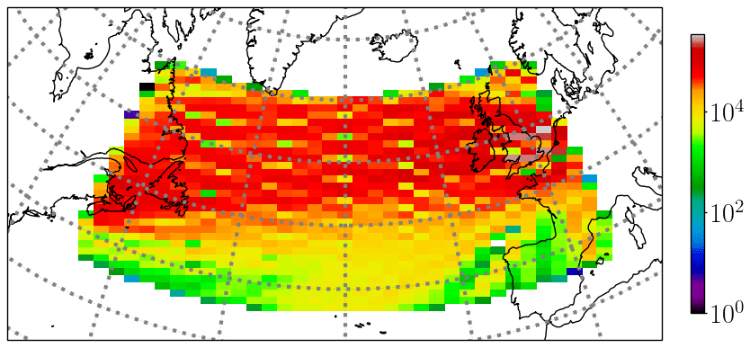
Figure 1Number of IAGOS measurements per grid box (2∘ in longitudinal and 0.57∘ in latitudinal directions) during 1 January 2000 to 31 December 2009.
2.2 ERA-Interim
For this study, the ERA-Interim reanalysis data set from ECMWF is used (Dee et al., 2011). The spectral resolution of the underlying IFS model from 2006 is T255, which calculates to a horizontal resolution of about 80 km in the midlatitudes. The vertical dimension is separated into 60 levels, reaching from the surface up to a pressure level of 0.1 hPa.
For the comparison with the IAGOS measurements, the 6-hourly ERA-Interim data were previously converted on a 1∘ horizontal grid and interpolated on pressure levels (Kunz et al., 2014). Then, the fields of temperature, pressure and specific humidity are projected on the aircraft's flight path by linear spatial and temporal interpolation. Finally, the data are available with a temporal resolution of 4 s along the flight track (Berkes et al., 2017).
The relative humidity with respect to ice was calculated using the approximation by Murphy and Koop (2005). As mentioned already in the introduction, the ERA-Interim data set was obtained by using the IFS model including the so-called Tompkins scheme (Tompkins et al., 2007), which allows for the supersaturation with respect to ice in cloud-free regions. However, inside cirrus clouds, the occurring supersaturation is adjusted down to 100 %. In the following, we use “ERA” to label the ERA-Interim data.
2.3 Methodology
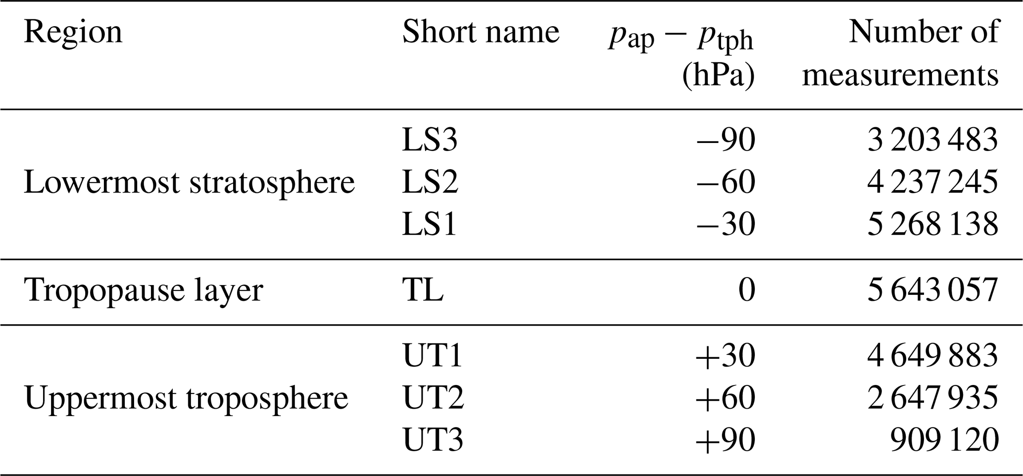
Aircraft-based measurements of atmospheric state variables and chemical composition usually refer to the aircraft flight altitude or pressure level, respectively. In the present work, the humidity data will be separated relative to the tropopause height in order to study the humidity in the tropopause region. We use the dynamical tropopause, which is defined by a sharp gradient in the potential vorticity (PV). The value used here to define the tropopause is PV = 2 PVU (1 PVU , standard potential vorticity unit) (Holton, 2005). A former study (Neis, 2017) showed that the choice of the tropopause definition can have an important impact on the interpretation of the results. However, in this study, we want to compare two data sets. Therefore, the definition of the tropopause plays only a minor role. The vertical data will be distributed into three main layers: upper troposphere (UT), tropopause layer (TP) and lower stratosphere (LS) in accordance with Thouret et al. (2006). Furthermore, UT and LS are each separated into three subclasses. The width of the sublayers considers the average difference between ozone and thermal tropopause of 780 m (30 hPa at this altitude) (Bethan et al., 1996). The resulting seven 30 hPa thick bins separate the aircraft pressure relative to the tropopause pressure and are summarized in Table 1.
Table 1The data set is distributed into three main layers: the upper troposphere, tropopause layer and lowermost stratosphere. The outer layers are additionally subdivided into three sublayers. The distribution criterion is the pressure difference between aircraft pressure pac and the tropopause pressure ptph with the range of ±15 hPa. Additionally, for every flight layer, the number of IAGOS measurements between 2000 and 2009 is presented.
Before the distribution of the data, several filters are applied. First, the measured data must lie within the geographic region from 40 to 60∘ N and −65 to 5∘ E. All data must be collected at a height above 350 hPa and within a temperature range between 233 and 200 K, corresponding to the threshold of homogeneous freezing (Heymsfield and Sabin, 1989) and calibration limit of the humidity sensor (Neis, 2017), respectively. Additionally, the relative humidity with respect to liquid water must be below 100 % and several measurement quality flags must be fulfilled. The abovementioned criteria are applied to both data sets and are the starting point of the comparison.
The aim of this section is to compare and quantify the difference of relative humidity with respect to ice (RHi) between the in situ measurements provided by IAGOS and the reanalysis data of ERA-Interim.
3.1 Temperature
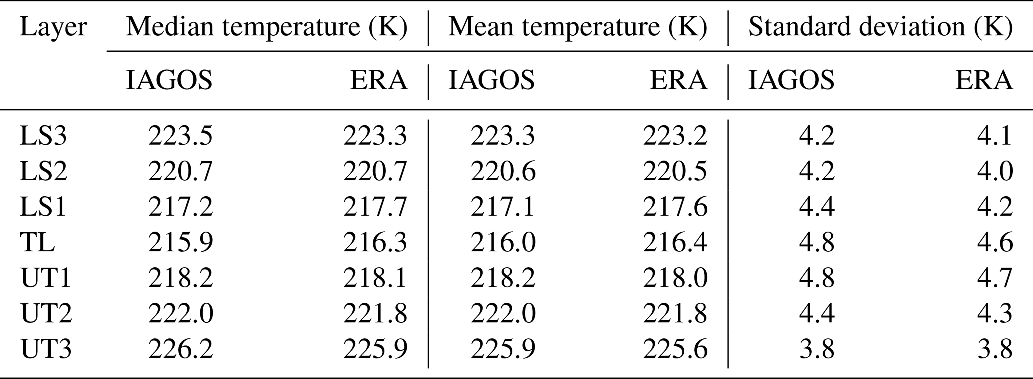
According to Eq. (1), the relative humidity depends on temperature and available water vapour. In a first step, a comparison between the temperature measurements and the reanalyses data for all seven height layers is conducted. Figure 2 shows the vertical profile of the temperature for IAGOS and ERA in the form of a box-and-whisker plot. The boxes are bounded by the 25th and 75th percentiles, while the median is marked with a vertical black line. The whiskers are defined as 1.5 ⋅ IQ, with IQ the interquartile range, equal to the distance between the 25th and 75th percentiles. Outliers, values exceeding the whiskers, are marked as black circles. As expected by definition, the tropopause layer shows the coldest mean temperatures, with 216.1 and 216.5 K for IAGOS and ERA, respectively. The warmest mean and median temperatures are visible for the lowest layer (UT3), with about 226 K in both cases. Overall, the comparison between IAGOS and ERA shows a very good agreement as far as the statistical values are concerned (see Table 2). This is supported by the equally sized boxes in Fig. 2, pointing to a similar variability of the data set.
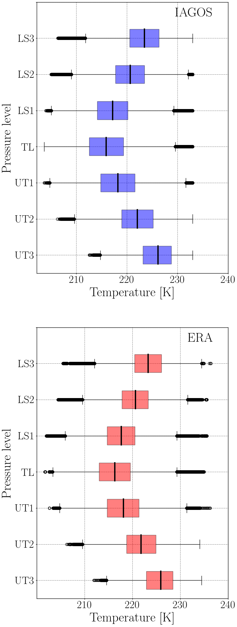
Table 2Median, mean and standard deviation of temperature (K) for IAGOS and ERA data. The comparison shows very good agreement.
3.2 Water vapour
The vertical structure of the water vapour volume mixing ratio is presented in Fig. 3. Here, a clear dependence of the distribution with height is visible. The lowest mean and median values of the water vapour volume mixing ratio are observed, as expected, in the uppermost layer (LS3). In contrast, the lowermost level (UT3) shows the largest mean values of the water vapour mixing ratio. The comparison between IAGOS and ERA shows a good overall agreement (see Table 3). For the upper layers, in both data sets starting from the tropopause level (TL) up to LS3, the variability, i.e. the size of the boxes, is significantly lower compared to the tropospheric layers (UT1 to UT3). Overall, it can be stated that the variability is increasing with decreasing height. It is notable that the outliers in all layers of IAGOS reach clearly higher mixing ratios than ERA. This has significant effects on the relative humidity with respect to ice, as will be shown later. In summary, the reanalysis data are in good agreement with the vertical distribution of the IAGOS data. However, IAGOS shows a larger variability and stronger extreme values.
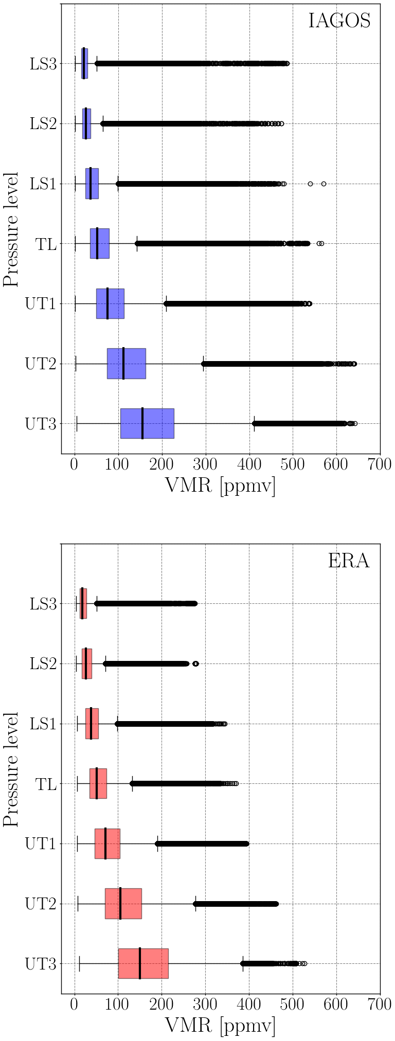
Table 3Same as Table 2 but for water vapour volume mixing ratio (VMR).

Dyroff et al. (2015) reported a moist bias comparing CARIBIC measurements with ECMWF analyses and forecasts. Since ERA-Interim is based on ECMWF analyses, one would expect also a moist bias in the lower stratosphere. In contrast to the capacitive sensor used for IAGOS, CARIBIC uses a combination of a frost point hygrometer and a photo-acoustic hygrometer, which shows a better precision and uncertainty for very low water vapour volume mixing ratios. Therefore, the uncertainties in volume mixing ratios of H2O are large in the lower stratosphere and may explain the more wet stratospheric values compared to CARIBIC. For more information, also see Petzold et al. (2019).
3.3 Relative humidity with respect to ice
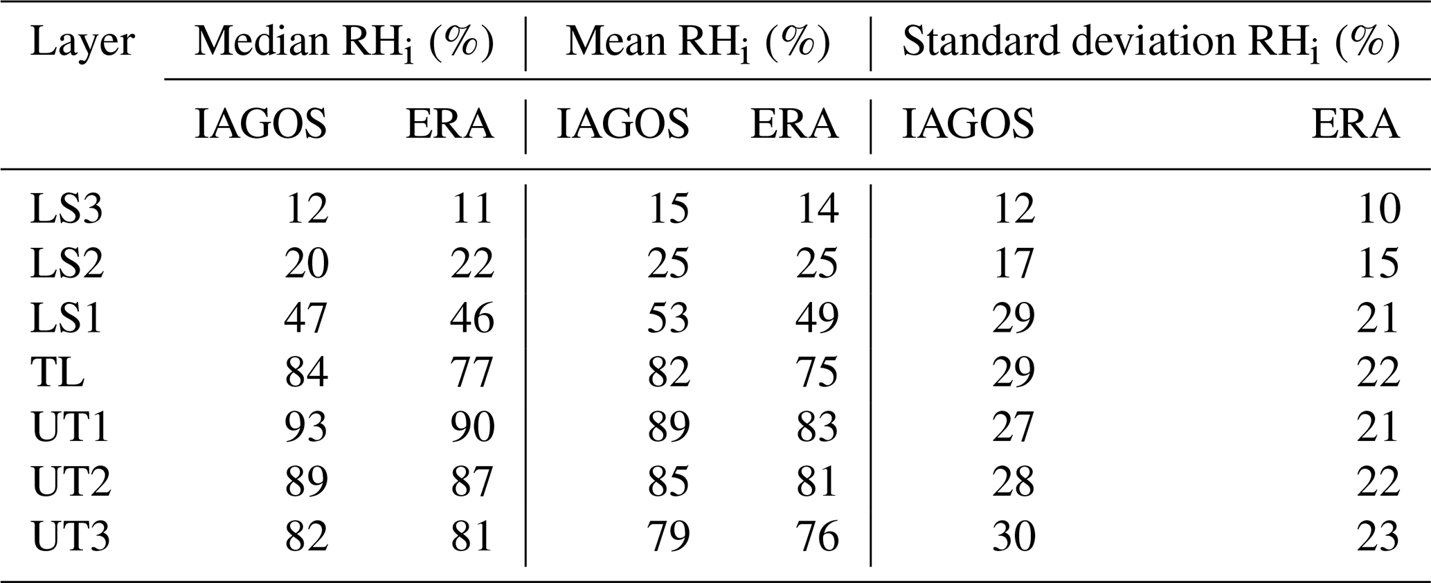
Since cloud formation is governed by the relative humidity rather than the water vapour mixing ratio, the relative humidity with respect to ice RHi is now investigated. As mentioned in the introduction, RHi depends on both temperature and available water vapour. Hence, relative humidity is a convolution of both variables. In Fig. 4, the vertical structure of RHi is depicted. The overall results show two different regimes. In the troposphere, up to the tropopause layer, the statistics cover the whole range of possible saturation values. Overall, 50 % of the data, indicated by the boxes, of each layer from UT3 to TL are situated between 50 % and 100 % RHi. The highest median values are found in the UT1 layer for both data sets (see also Table 4). In the tropopause layer, still a significant amount of the data is exceeding values of RHi>100 %, both in the in situ data as well as in the ERA data set. However, the whisker in Fig. 4 indicates that ERA has less data points with a higher supersaturation compared to IAGOS. In the stratospheric layers, the median of the RHi values is decreasing strongly. However, ice supersaturation is still possible, especially in the lowest stratospheric layer (LS1) (Müller et al., 2015). The statistics of ISSRs in higher levels provided by the ERA data set show clearly less occurrence of this feature. Since ISSRs are an important factor for the formation and lifetime of contrail cirrus (Kärcher, 2018), a good model representation of the abundance of ice supersaturation in this region is important for an adequate description of the Earth's radiative budget.
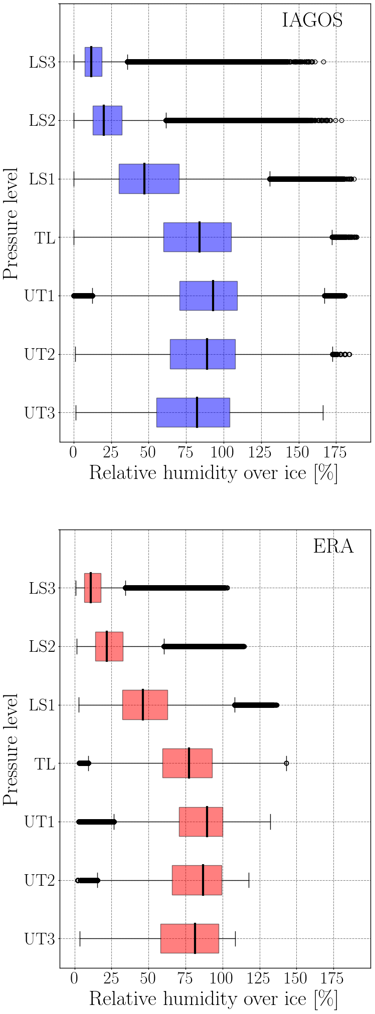
Figure 4Vertical profile of relative humidity with respect to ice (RHi) (%) for IAGOS (blue) and ERA (red).
It is obvious that ERA and IAGOS show good agreement for situations below ice supersaturation. However, in this study, we focus on the situation where ice supersaturation exists. For a more distinct look at the occurrence of ISSR, we illustrate the statistic evaluation with cumulative probability in Fig. 5. Each layer is depicted with its own colour. It is clearly visible that ERA and IAGOS behave differently for RHi>100 %, especially for the tropospheric layers. The ERA distributions of the latter layers snap off as soon as they reach ice supersaturation. As mentioned before, the IFS model allows the existence of ice supersaturation but only in cloud-free conditions. As soon as ice clouds are present in the model's grid cell, the supersaturation is adjusted to RHi=100 %. Unfortunately, the IAGOS data set of the investigated timeframe cannot distinguish between cloudy and non-cloudy areas. 1 Nevertheless, also in ice clouds, ice supersaturation is present (Krämer et al., 2016). Therefore, the behaviour of the cumulative distributions for ERA, especially in the layers from UT3 to TL, might be due to an untimely formation of ice clouds in the underlying IFS model, which adjusts the ice supersaturation too early.
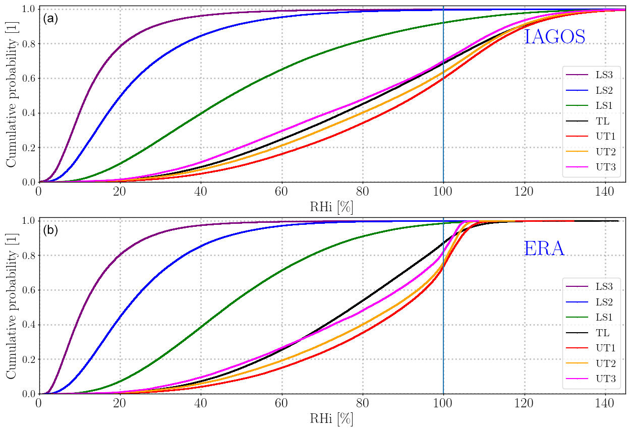
Figure 5Cumulative distribution of RHi for every height level in the IAGOS (a) and ERA (b) data sets. The vertical blue line denotes saturation with respect to ice.
Another way to compare the representation of the water vapour is the fraction of ISSRs. Figure 6 presents the vertical profile of the ISSR fraction. The ISSR fraction in this study is defined as the number of data points within a layer with RHi≥100 % divided by the total number of data points in that layer above the defined North Atlantic region. It is clearly visible that the measurements by IAGOS show a higher fraction of ISSR. Only for the two uppermost layers, the fractions of both data sets are of comparable magnitude. Here, the very dry conditions produce supersaturation only in very few cases. The largest difference between measurement and reanalysis data occurs in the tropopause layer and the flanking UT1 layer, where a high percentage of ice clouds can be expected. IAGOS shows in the latter layer an ISSR fraction of up to 40 %. Since ISSRs are a prerequisite for the formation of in situ cirrus clouds, a misrepresentation of the feature can lead to great deviations in the local radiative budget and can build up to large errors in the local dynamics. However, sensitivity studies were conducted in order to see if ERA can reproduce the ISSR fraction of IAGOS using a lower threshold than RHi=100 %. For each layer, a different threshold for the ERA data set leads to the best agreement with IAGOS. The best comparison between IAGOS and ERA in the lower stratosphere is found when ice supersaturation in ERA is defined as % (dotted red line in Fig. 6). For the tropopause layer, the best agreement is found for % in ERA (dash-dotted line), while the upper troposphere shows an almost perfect match for % in ERA (dashed line). This shows that the agreement between measurement and reanalysis is decreasing with increasing height. One reason might be the data assimilation of measurements into the reanalysis data set. The operational radiosondes using capacitive sensors (usually RS80 and RS92 with Humicap sensor by Vaisala) show large deviations for temperatures below −40 ∘C or very low absolute humidities (Spichtinger et al., 2003a). Therefore, the response time is increasing in the upper troposphere to the tropopause layer due to the decreasing temperature. Further up in the stratosphere, temperatures are increasing again (Fig. 2). However, the absolute humidities are decreasing with height (Fig. 3), leading to an increased response time.
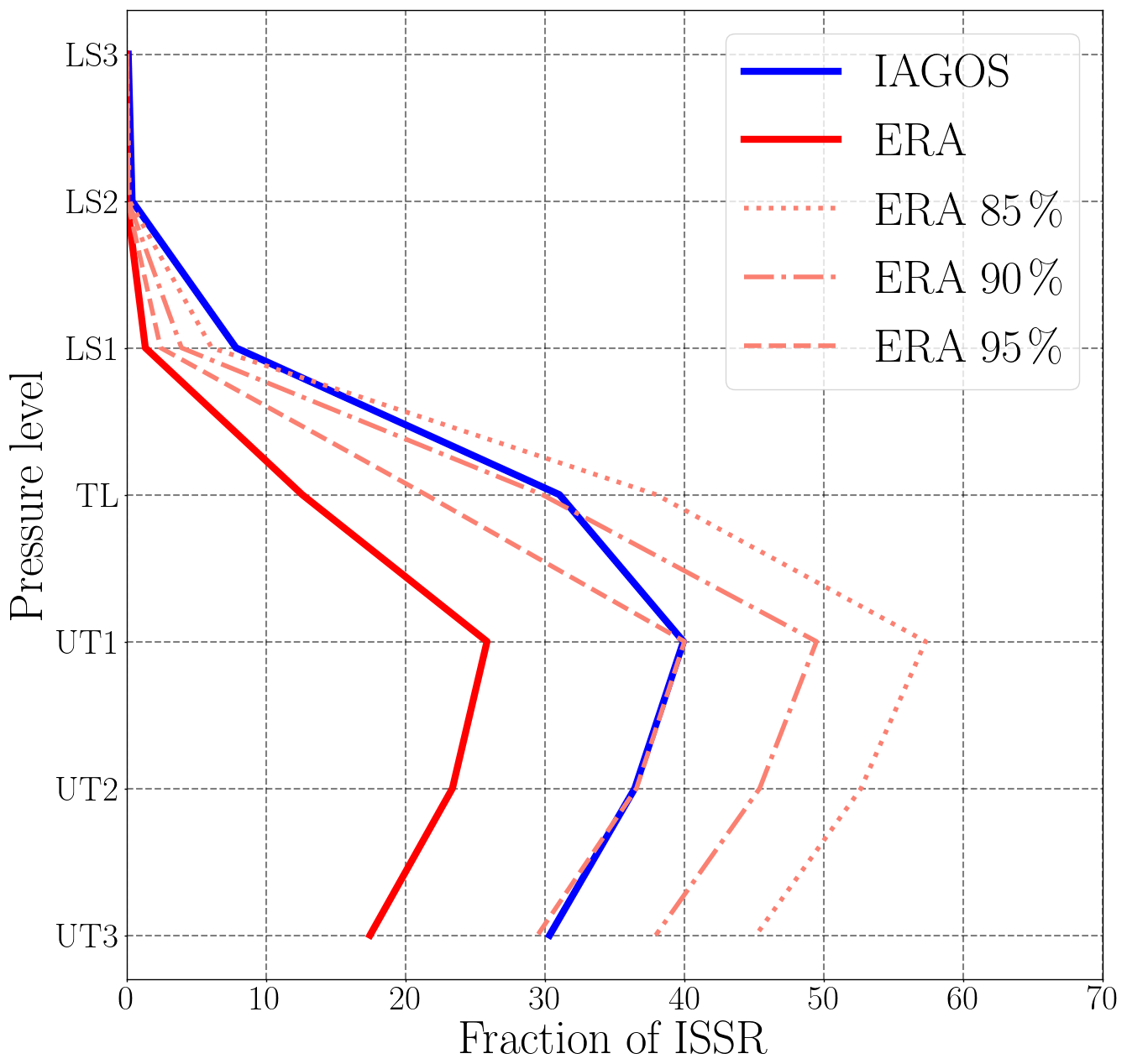
Figure 6Vertical profile of the fraction of ice supersaturated regions for IAGOS (blue) and ERA (red). Different definitions of ice supersaturation in ERA are shown in light red. The dotted line represents the fraction of % , the dashed–dotted line depicts the fraction of %, and the dashed line stands for the %.
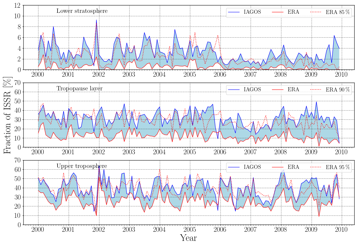
Figure 7Time series of the monthly fraction of ice supersaturated regions for IAGOS (blue) and ERA (red) for the lower stratosphere (LS1 to LS3), the tropopause layer TL and the upper troposphere (UT1 to UT3). The dashed red line represents the ERA data set with the fraction of RHi≥85 % for the lower stratosphere, RHi≥90 % for the tropopause layer and RHi≥95 % for the upper troposphere. Note the different scale for the lower stratosphere.
In contrast to the total fraction over the complete period from 2000 to 2009, Fig. 7 shows a time series of the monthly ISSR fraction. For this comparison, the three stratospheric (tropospheric) layers were combined to one layer defined as “lower stratosphere” (“upper troposphere”). The dotted lines in Fig. 7 indicate the fraction of data points for % in the lower stratosphere, for % in the tropopause layer and for % in the upper troposphere, respectively. Note that the variation of the ISSR fraction is not only affected by meteorology but also due to different data coverage. For instance, at the end of 2001, only few data points are available, which explains the prominent spikes in the lower stratosphere and upper troposphere. Comparing the time series with Fig. 6, it is again visible that ERA is underestimating the fraction of ISSR compared to the measurements from IAGOS. Using a different definition of ice supersaturation by reducing the threshold in ERA (85 %, 90 % and 95 %) improves the agreement between ERA and IAGOS in each layer. However, the different thresholds can also lead to overestimation of the ISSR fraction. While in the lower stratosphere, a threshold of % shows a overall good agreement, in 2005, this threshold would lead to an overestimation of the ISSR fraction of up to 300 % (December 2005). It is also noteworthy that, although Fig. 6 shows an almost perfect agreement between IAGOS and the modified threshold of 95 % in the upper troposphere, large deviations between IAGOS and ERA can be found as well, for example, in 2004.
As a side note, the reader is referred to the companion study by Petzold et al. (2019), where also a trend analysis using the IAGOS data was conducted, which led to the conclusion that no significant trends in ISSR occurrence can be observed. However, they do find a correlation between the North Atlantic Oscillation (NAO) and ISSR occurrence.
Although ISSRs are three-dimensional fields, the measurements only provide one-dimensional pathlengths. Therefore, only these pathlengths can be used to characterize the size of ice supersaturated regions. We are also interested in the seasonal cycle and height dependence of ISSR pathlengths. Also, the distance between two neighbouring ISSRs is of interest. Additionally, these properties are compared to the reanalysis data and previous studies.
Former studies (Diao et al., 2014; Spichtinger and Leschner, 2016) showed that the horizontal pathlengths can reach from the very small scale on the order of hundreds of metres to up to 1000 km. Here, small-scale variability will lead to very short ISSRs, while large-scale features will produce large ISSR pathlengths.
Figure 8 presents an exemplary flight from Atlanta (USA) to Frankfurt (Germany) on 7 March 2009. Blue shows the high-resolution data available from the IAGOS database. Red marks the ERA data obtained from the given flight track, and the black line shows the pressure level of the airplane. Shaded areas are blue for ice supersaturation in the IAGOS data set and red for ERA. In the upper part of Fig. 8, a satellite image from 7 March 2009 can be seen. Note that the flight landed at 07:52 UTC, while the satellite image is taken at 12:00 UTC; therefore, a shift between measurements and image has to be kept in mind. A low pressure system, located between the British Isles and Iceland, is dominating the weather over the North Atlantic. The warm conveyor belt (WCB), an ascending airflow from the boundary layer to the upper tropopause (Spichtinger et al., 2005), with its cloud band is clearly visible, reaching from Ireland to the southwest. Between a flown distance of 5000 to 6000 km, an increase in the relative humidity with respect to ice is shown, both in IAGOS and ERA. This is in agreement with other studies, where cirrus clouds and ice supersaturation are found in the ascending air masses of the warm conveyor belt (Spichtinger and Leschner, 2016). Behind the cold front, a region of post-frontal showers is visible. This is the region of the dry intrusion (Browning, 1997), where stratospheric dry air can be expected at the cruising altitude of the airplane. This can be clearly seen by comparing the height of the airplane (black) and the height of the dynamical tropopause (green) between a flown distance of 4000 and 5000 km. The tropopause decreases down to a height of 500 hPa, and RHi reaches very low values.
The overall agreement between measurement and reanalysis is quite good when focusing on the patterns of large-scale variability. It is obvious that ERA, due to the coarse model resolution, is not able to reproduce the very small fluctuations as seen in the IAGOS data. While the first ISSR after start is reproduced by ERA at the right location, the ISSR at a flown distance of about 6000 km is misplaced compared to IAGOS. It can also be seen that the pathlength of the first ISSR is significantly larger in ERA. Note that for this study only ISSRs within the North Atlantic region of this specific flight are taken into account.
In the following, we will focus on the length of ISSRs. Therefore, we start with a statistical comparison of the pathlengths between IAGOS and ERA. Here, the influence of the spatial resolution on the statistics of ISSR pathlengths is investigated. After that, we use the unique IAGOS data set to study in more detail the dependence of ISSR pathlengths on the season and atmospheric layer, i.e. the differences between the lower stratosphere, tropopause and upper troposphere.
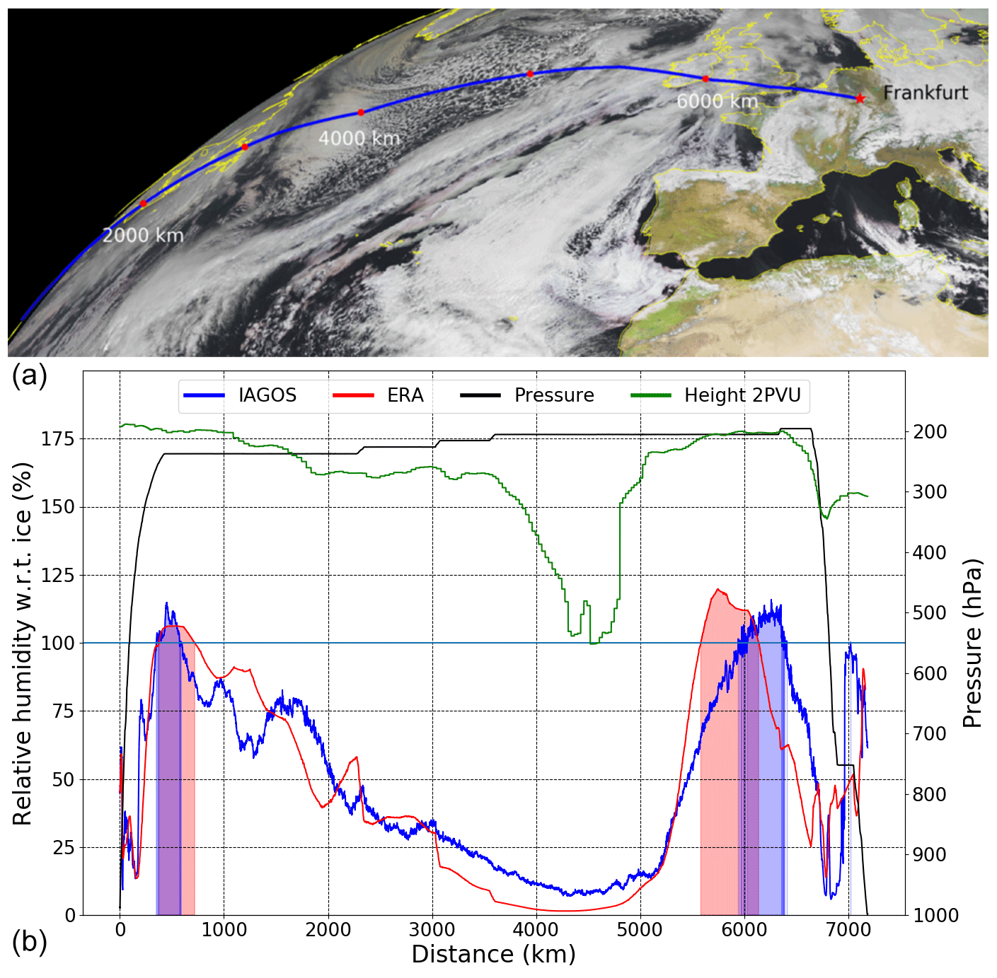
Figure 8Example of a typical flight from Atlanta (USA) to Frankfurt (Germany) on 7 March 2009. The upper part shows the synoptic situation over the North Atlantic on that day including the flight path. For better orientation, red dots are placed every 1000 km. In the lower part, RHi is shown over the distance of the flight for IAGOS (blue) and ERA (red). Shaded areas denote ice supersaturation. The pressure level of the aircraft is shown in black, and the height in hPa of the dynamical tropopause (2PVU) is shown in green. Satellite image: © 2009 EUMETSAT.
4.1 Statistic investigation of ISSR pathlengths
It is obvious that the smallest possible pathlength of the ERA data set is limited by the model's spatial resolution. However, by calculating a moving average of the IAGOS data close to the ERA resolution, a comparison is possible. Additionally, we want to answer the question of which resolution is necessary in order to receive a helpful representation of the horizontal scales of ISSRs. A comprehensive representation of ISSRs in atmospheric models enables further investigations on the linkage between small-scale variability and large-scale features.

Figure 9Probability of ISSR pathlengths with logarithmic binning (a) and cumulative probability (b). The original IAGOS data are shown in black, while ERA is presented in red. Other colours denote different running means of the original IAGOS data set to mimic different spatial data resolution.
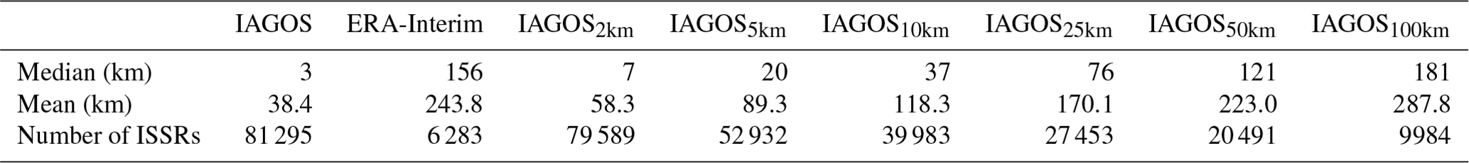
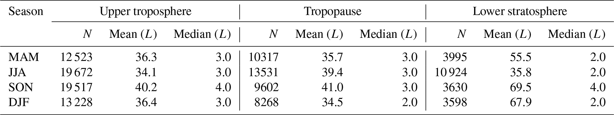
For a reasonable comparison of ISSR pathlengths between IAGOS and ERA, we only evaluate ISSRs on a constant flight level. This means that an ISSR path is omitted if the pressure level of the plane is changed by more than 50 Pa. Figure 9 shows the histograms for the pathlengths of IAGOS and ERA, and running means of 2, 5, 10, 25, 50 and 100 km of the IAGOS data. On the right side, a cumulative distribution is shown. As it is expected from the different underlying resolutions of both data sets, IAGOS (black lines in Fig. 9) shows a much greater number of small pathlengths compared to ERA (red lines). On the other side, ERA shows a greater number of very large pathlengths larger than 100 km. This is especially impressive by looking at the cumulative distribution. Here, the different character of both data sets is most prominent. Comparing the median values given in Table 5 of the original IAGOS data and ERA reveals the big difference. While 50 % of the ISSR pathlengths in IAGOS are smaller than 3 km, the same threshold for the ERA data set is located at 156 km. It has to be noted that due to the lower spatial resolution of the ERA data set, only 6283 ISSRs are found compared to 81 295 for IAGOS.
Table 5Median and mean values and number of ISSR pathlengths for IAGOS, ERA-Interim and several running means of the original IAGOS data set.
Previous studies also investigated pathlengths of ISSRs. Diao et al. (2014), hereafter D14, investigated ISSR from very-high-resolution measurements (1 Hz ≈230 m) using data from several flight campaigns. They report a mean ISSR pathlength of 3.5 km, while the median value is about 0.7 km, with a total number of 1542 ISSRs. These values are about 1 order of magnitude lower compared to our investigations. However, these data include measurements from 87∘ N to 67∘ S and therefore include tropical conditions.
Spichtinger and Leschner (2016), hereafter SL16, used MOZAIC data from 1995 to 1999 with an original resolution of about 14 km and artificially decreased the resolution to 100 km. They report a mean pathlength of 122 km and a median value of 55 km for the original data, which are close to our results of IAGOS with a running mean of 10 km. The coarse resolution of SL16 has a mean pathlength of 247 km and a median value of 149 km. These values are between our results for the running means of 50 km and 100 km of the IAGOS data. Additionally, the SL16 coarse data are in very good agreement with the mean and median of the ERA-Interim data.
The comparison of the mean and median values with D14 and SL16 showed that the results differ due to the underlying resolution of the measurement data. For every scale, a different conclusion can be drawn. Therefore, the question arises as to which resolution is feasible to describe the ice supersaturation in a sufficient realistic way for a certain scale. Already with a resolution of 2 km, the number of small ISSRs is decreasing strongly. The median value increases to 7 km, compared to the original resolution. Decreasing the spatial resolution further leads to a decrease in the number of found ISSRs and an increase of the mean and median ISSR pathlengths. At a resolution of 10 km, the cumulative distribution exhibits a different character compared to the original data. When reaching a running mean of 100 km, which is around the spatial resolution of the ERA data set, the numbers of found ISSRs and median pathlength are on the same order of magnitude as the reanalysis data. When comparing the results of the 100 km running mean of IAGOS with the ERA data set, it is also noteworthy that the behaviour for ERA is clearly different for pathlengths smaller than 100 km. ERA shows a significantly higher probability for very small ISSRs (<10 km) than the running mean with 100 km. However, the increase in probability to pathlengths of up to 100 km is flatter in ERA. Again, as a reminder, this is the scale of the spatial resolution of ERA.
It is clear that the ISSR with pathlengths smaller than 100 km is not represented in the ERA model in the same way that the running mean of IAGOS shows it. At first, this discrepancy may look small. However, as mentioned before, small ISSRs also can have a profound effect as a formation region of cirrus clouds. The impact of these smaller ISSRs on the larger scale by changing the dynamics around the tropopause is not clear yet.
4.2 Seasonal cycle and height dependence of ISSR pathlengths
The previous results showed the overall statistics of ISSR in the North Atlantic region. Fortunately, the data set allows for a more sophisticated investigation of ISSR properties such as seasonal cycle or height dependence. Therefore, the seasonal cycle for the lower stratosphere, tropopause and upper troposphere is presented in Fig. 10 for IAGOS and ERA. For the sake of clarity, we combine the three upper levels to “lower stratosphere” and the three lower layers to “upper troposphere”. Starting with spring (MAM), the cumulative distribution shows that for IAGOS in the lower stratosphere and the tropopause region a higher fraction of short ISSRs is present than in the upper troposphere. Up to 75 % of the ISSRs in the lower stratosphere and the tropopause region are smaller than 10 km. The upper troposphere shows the highest fraction of pathlengths between 10 and 100 km. In the lower stratosphere, pathlengths larger than 100 km are more common on a percentage basis compared to the tropopause and upper troposphere layers.
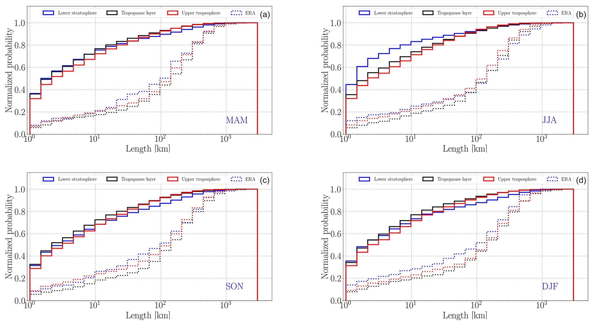
Figure 10Seasonal cycle of ISSRs for lower stratosphere (blue), tropopause (black) and upper troposphere (red). Dashed lines show results for ERA. Panels (a) and (b) represent spring and summer months; (c) and (d) represent fall and winter months, respectively.
A clearly different result is visible during the summer months (JJA) in the lower stratosphere. Overall, 60 % of the ISSRs are smaller than 2 km and over 80 % smaller than 10 km. The special conditions for the stratosphere in summer are also visible in the statistical values shown in Table 6. While the mean pathlength in the stratosphere for spring is around 55 km, this value decreases to 35.8 km in summer, before an increase to approximately 70 km in fall and winter is observed. It has to be noted that the number of ISSRs in the stratosphere during summer is over 2 times higher compared to the other seasons.
Table 6Number (N), mean and median of ISSR pathlengths L (km) for the upper troposphere, tropopause and lower stratosphere for the MAM, JJA, SON and DJF seasons.
It is not clear what kind of process is responsible for the large amount of small ISSRs during summer in the lower stratosphere. In principle, relative humidity with respect to ice can be altered by a change of temperature, pressure or specific humidity. Processes behind these changes can be especially adiabatic expansion or mixing of different air masses. SL16 investigated the origin of small-scale ISSRs and concluded that most of the variation of RHi is due to adiabatic processes, i.e. cooling by expansion. This means that the transport of air masses from different altitudes creates small-scale variations of RHi in the region from the upper troposphere to the lower stratosphere. However, a deeper investigation of this question requires three-dimensional data and trajectory analysis, which are not in the scope of the present study but should be conducted in the future.
The results for fall (SON) and winter (DJF) are very similar. The tropopause region shows the highest percentage of ISSRs with a pathlength smaller than 10 km. Pathlengths between 10 and 100 km show the highest fraction in the upper troposphere, while the highest percentage of ISSRs with sizes larger than 100 km can be found in the lower stratosphere.
The results for ERA (dotted lines) in spring, and also for the other seasons, are clearly different. As mentioned above, short ISSRs are underestimated by ERA due to the spatial resolution, which is visible for all seasons. The different resolution leads also to other relations of the pathlengths between different height levels. For instance, the highest fraction of ISSR in spring with a pathlength between 10 and 100 km is found in the lower stratosphere. This behaviour is reversed compared to the IAGOS data set, where the upper troposphere showed the highest fraction. The same observation can be made in winter as well. Not surprisingly, ERA misses also the high fraction of short ISSRs in the stratosphere during the summer season.
In general, the mean pathlength of an ISSR in the IAGOS data set is significantly larger in the stratosphere compared to the upper troposphere and tropopause layer, except for the summer season, which is also shown in Fig. 11. Comparing the mean pathlengths for every season in the IAGOS data makes clear that the strongest seasonal cycle is present in the lower stratosphere, with the lowest mean pathlength in summer and the highest values in fall and winter. This might be due to the enhanced storm track activity during fall and winter, where the mass flux (including water vapour) from the troposphere to the stratosphere is largest (Reutter et al., 2015). Further investigations are needed to answer this question.
The two lower layers also show a seasonal cycle, however with a smaller amplitude and shorter absolute mean values. While the upper troposphere also shows the shortest mean pathlength in the summer, the minimum in the tropopause is found during winter. Note that, due to the large number of very small pathlengths in all seasons and all levels and the logarithmic binning of the results, the median values show only a small interseasonal fluctuation. Figure 11 also shows the seasonal cycle of the mean and median pathlengths for the ERA data set. As expected, due to the large resolution of the data set, also the mean and median values are significantly larger compared to IAGOS. More importantly, the seasonal cycle of ERA is shifted, especially for the tropopause and lower stratosphere. The maximum mean pathlength in the tropopause can be found in summer for IAGOS, where, in the ERA data, the minimum pathlength is found. The same holds true for the lower stratosphere, where the minimum for IAGOS is also found in summer, where ERA exhibits the maximum. Additionally, the relative amplitude of the seasonal cycle is smaller compared to IAGOS, most prominent in the lower stratosphere. Here, also the spread of the data, indicated by the size of the boxes, shows a large fluctuation in the IAGOS data set, which is not captured by ERA.
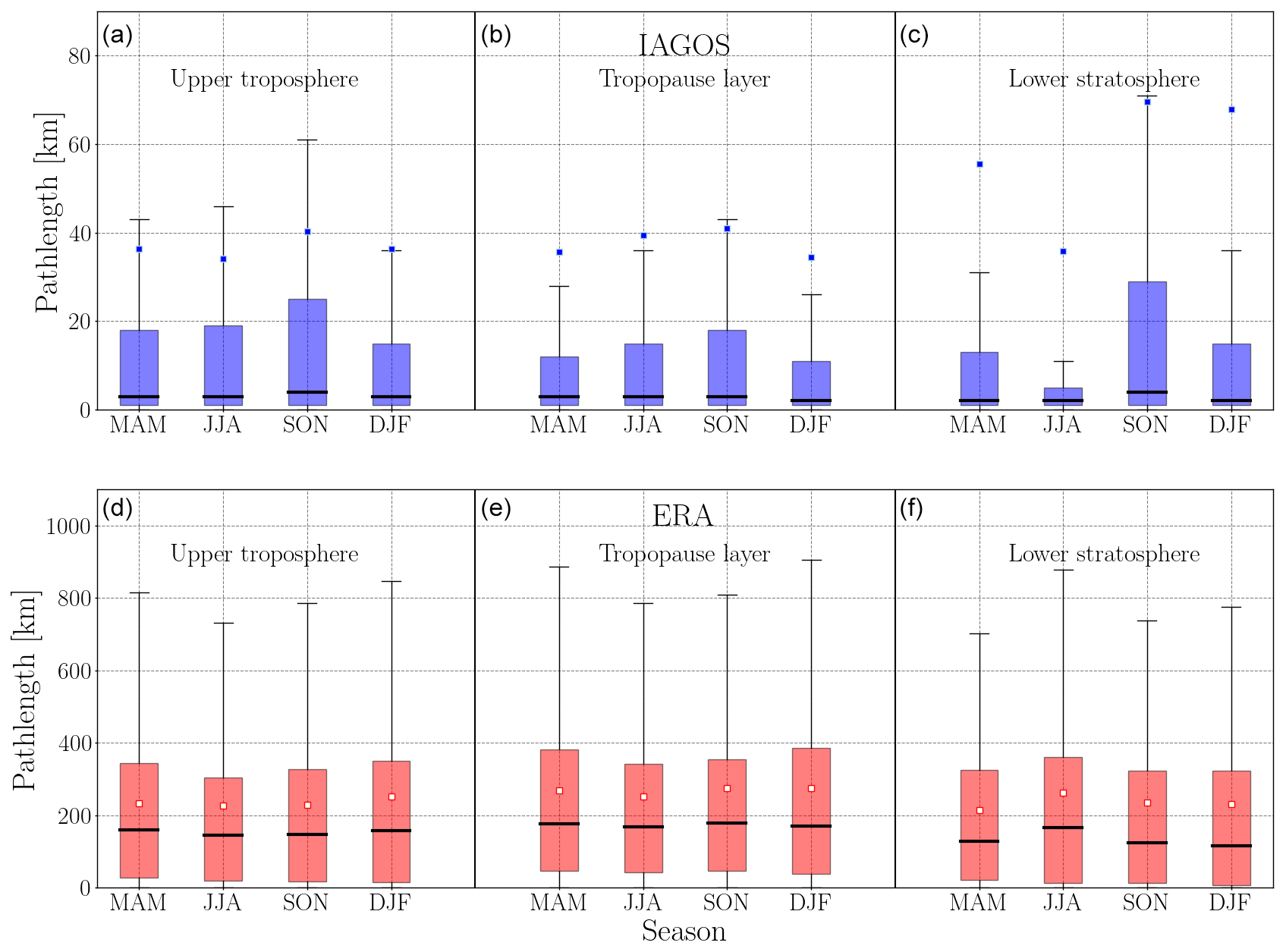
Figure 11Box-and-whisker plot of the seasonal cycle of pathlengths of ISSR for different atmospheric layers in IAGOS (a–c) and ERA (d–f). For each box, the squares denote the mean pathlength and black lines the median pathlength, respectively.
SL16 also investigated the seasonal cycle of ISSRs. All ISSRs of the extratropics (latitude ≥30∘) were separated into “troposphere”, “stratosphere” and “in between” using the ozone mixing ratio. This chemical definition of the tropopause is close to the thermal definition. However, in our study, we use the dynamical definition of the tropopause. This has to be kept in mind for the interpretation of the comparison. As mentioned above, the data used in SL16 showed a coarser resolution of about 1 min (which converts to about 14 km depending on the true air speed of the plane) in contrast to the much higher 4 s (about 1 km) resolution in this study. They focused on the large-scale aspects of ISSRs, and therefore the original data were analysed with a coarse resolution (realized with a running mean of the original data) of about 100 km. The coarser resolution makes a quantitative comparison difficult, since already 60 %–80 % of the ISSRs in our study are smaller than 10 km, i.e. below the spatial resolution of the original data in SL16. The maximum of the mean pathlength in SL16 for the stratosphere is found in winter, while the minimum is found in fall. This is in contrast to the finding in the present study, where, on the one hand, in winter also the maximum pathlengths are found, but the minimum is found in summer. Additionally, during fall, about the same mean pathlength can be found as in winter. The comparison of the seasonal cycle for the tropopause layer between SL16 and the present study also reveals a shift. The maximum mean pathlength in SL16 is found in fall, where our study detects the maximum in summer. The seasonal cycle in the tropospheric layer in SL16 and the present study is in good agreement.
It seems that the difference in the seasonal cycle between SL16 and our study can be, to a large fraction, attributed to the spatial resolution of the data. Figure 11 shows also the seasonal cycle for ERA, where the agreement with SL16 is better. Also, as mentioned in the discussion of Table 5, the agreement between ERA, the running mean of 50 and 100 km, as well as the results of SL16, is very good. Therefore, it is important to have the awareness that the spatial resolution can strongly influence the results of ISSR pathlengths.
4.3 Seasonal cycle and height dependence of the distances between ISSRs
Finally, we present the seasonal cycle of the distance between two neighbouring ISSRs. Figure 12 shows the cumulative distributions of the distance between ISSRs for IAGOS and ERA, while in Table 7 the statistical overview for IAGOS is given. Here, a clear seasonal cycle is visible in all three layers, in contrast to the pathlengths of ISSR. For all layers, the maximum of the mean distance is found in fall, with the largest value of 79.1 km in the lower stratosphere and the smallest distance in the upper troposphere with 55 km. The shortest mean distances are found in winter for all layers with values from 35.3 km in the upper troposphere to 40.3 km in the lower stratosphere.
Table 7Mean and median of the distance D (km) between ISSRs in the IAGOS data set for the upper troposphere, tropopause and lower stratosphere for the MAM, JJA, SON and DJF seasons.
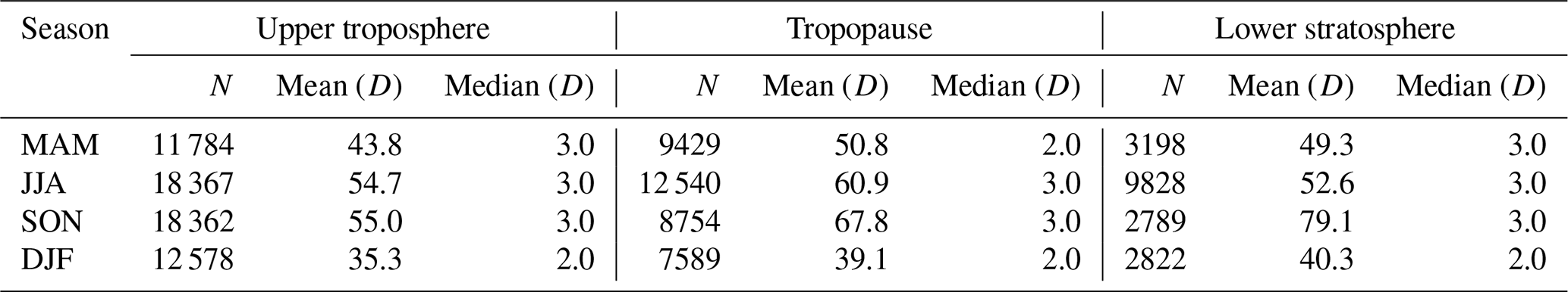
A shorter mean or median distance implies that ISSRs are closer to each other (D14). Therefore, in winter, the conditions favour ISSRs with smaller distances. This also suggests that in the upper troposphere and the tropopause region, where the interseasonal mean pathlength of ISSR does not change strongly, the structure of ISSR is more heterogeneous than in other seasons. For the lower stratosphere, one has to keep in mind that the mean pathlength in winter is, together with fall, significantly larger than in spring or summer. Therefore, not only is the distance between ISSRs shortest, but also the pathlength is largest.
In D14, the authors presented a mean distance between ISSRs of about 47 km, while the median distance is approximately 1 km. These values are in good agreement with our findings. However, as mentioned before, D14 used global data without the distinction between geographical region or height. SL16 also investigated the distance between ISSRs. The mean and median values are significantly larger than in the present study, which is, again, due to the different spatial resolution. Also, as for the ISSR pathlength, the seasonal cycle is shifted compared to the higher resolution in our work.
The results for ERA (dotted lines in Fig. 12) show again a clearly different picture. The comparison of the height dependence between IAGOS and ERA reveals a reversed and even enhanced dependence as it is shown by the distance of the vertical layers within the ERA data set. For instance, in winter, the reversed dependence with height is most prominent. Between 1 and 100 km, the lower stratosphere shows the highest fraction of distances, followed by the tropopause layer and the upper troposphere. In ERA, this dependence is the opposite, with the highest fraction in the upper troposphere and the lowest fraction in the lower stratosphere.
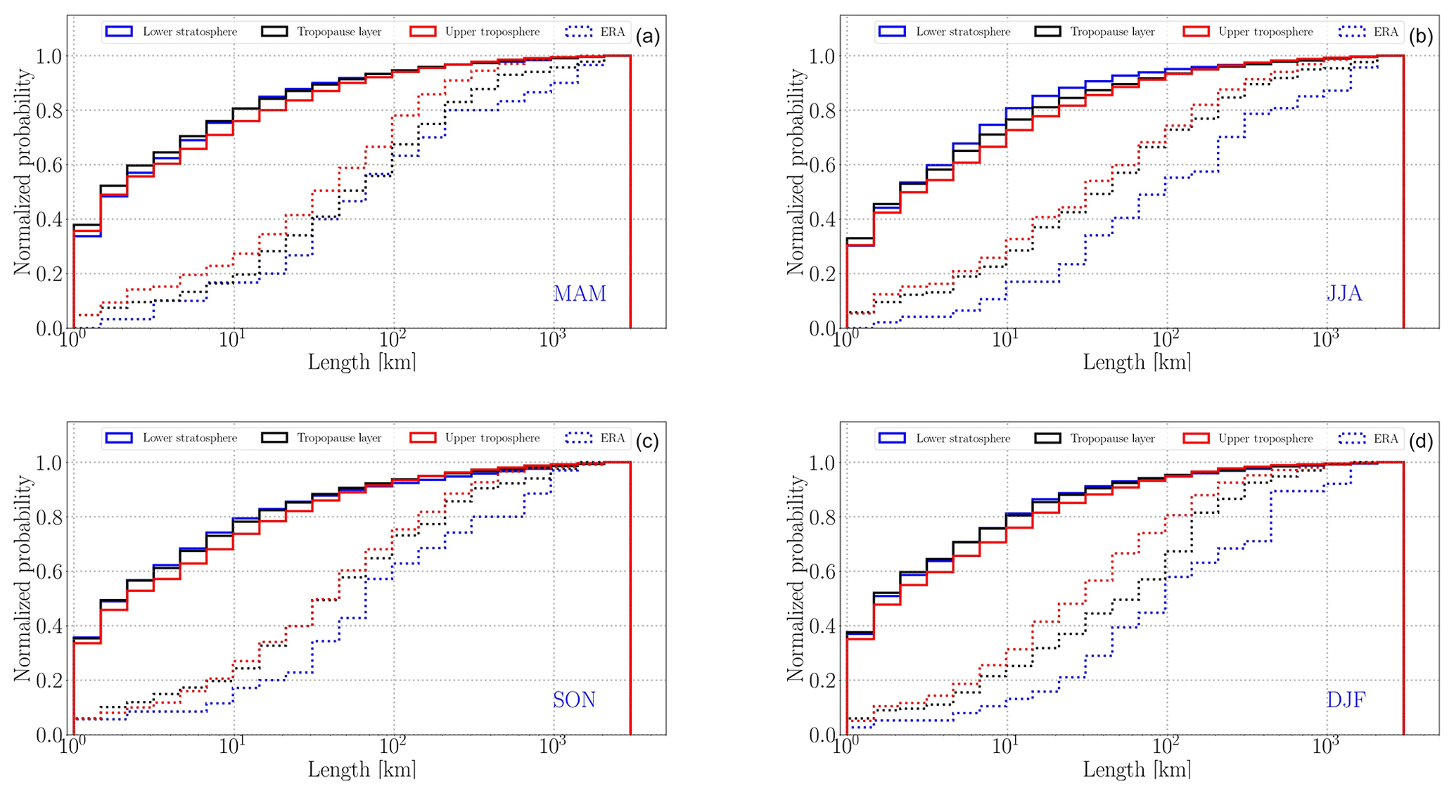
Figure 12Seasonal cycle of the distance between ISSRs for lower stratosphere (blue), tropopause (black) and upper troposphere (red). Dashed lines show results for ERA. Panels (a) and (b) represent spring and summer months; (c) and (d) represent fall and winter months, respectively.
This study compares the in situ measurements of temperature and water vapour and subsequent relative humidity with respect to ice in the UTLS region obtained by IAGOS with the ERA-Interim reanalysis data set from the years 2000 to 2009 over the North Atlantic. Ice supersaturated regions (ISSRs) are of special interest in this investigation due to their abundance and importance on the local radiation budget when transformed to a cirrus cloud. Additionally, the characteristics of the horizontal scale of ISSRs are investigated, including the seasonal cycle and height dependence. Both data sets are separated according to their relative height compared to the dynamical tropopause (2 PVU). The comparison of the temperature shows good agreement between measurement and reanalysis data. The structure and variability of the vertical temperature distribution are very similar, shown by very good accordance in median and mean values as well as in the standard deviation. The water vapour was analysed using the water vapour mixing ratio. Both data sets show the clear decrease of water vapour with increasing height. In contrast to the measurements, ERA shows clearly less variability, indicated by smaller standard deviations in all levels. The convolution of water vapour and temperature leads to the relative humidity with respect to ice, which governs the cloud formation. Both data sets reproduce two different regimes. In the UT layers, including the tropopause layer, the statistics cover the whole range of possible saturation values, where most of the data lie between 50 % and 100 % RHi. However, ERA deviates from the RHi measurements concerning values larger than RHi=100 % by showing less data points and weaker supersaturations, impressively depicted by the comparison of cumulative distributions. This is an important finding, because it points to a misrepresentation in ERA of ice supersaturation in the UT and tropopause region, which is the formation region of in situ cirrus. Moving up to the stratospheric layers, the RHi values, as expected, are much lower in both data sets. Again, ERA shows less and weaker supersaturations through all levels. Since the LS is very dry, supersaturation occurs rarely, and therefore the difference between both data sets is smaller regarding the cumulative distribution. Nevertheless, ERA shows clearly less extreme events. The strong differences between IAGOS and ERA with respect to ISSRs is also shown by the fraction of ISSR. In the UT and the tropopause region, the measurements show a significantly larger fraction of ISSR in the measurements compared to ERA.
The comparison of pathlengths of ISSRs clearly shows the different resolutions of the two data sets. It is obvious that the high-resolution measurements show more small ISSRs than ERA. Only beginning with pathlengths on the order of 100 km, the distribution starts to have a similar course. This length scale coincides with the horizontal resolution of the underlying ERA model. Decreasing the resolution of the IAGOS data by running means shows only a good agreement of model and measurement beginning with a running mean of 100 km, which is, as stated, on the order of the model resolution. However, even in the latter case, the structure of the distribution of ISSR smaller than 100 km is clearly different between IAGOS and ERA. Therefore, a simple increase of the model resolution seems insufficient. Additionally, the physical processes must be refined carefully for a realistic description of the ice supersaturation in the UTLS region.
The investigation of the horizontal scales of ISSRs provides several results. First, the high-resolution data from IAGOS showed a very high percentage of small-scale ISSRs, which is highlighted by median values between 2 and 4 km for all heights during all seasons. Up to 80 % of the ISSRs are smaller than 10 km. The seasonal cycle of the ISSR pathlengths is small for the upper troposphere and tropopause regions but shows a distinct change for the lower stratosphere during the course of the year. Here, during summer, the mean pathlength of an ISSR is lowest with 35.8 km compared to the maximum during fall with 69.5 km. The comparison with previous studies using different spatial resolutions as well as ERA showed that the characteristics of the horizontal scale strongly depend on the data structure. Not only the statistical values like mean and median values differ strongly, but also the seasonal cycle is shifted when using different resolutions. Additionally, the sign of the height dependence is changed when comparing IAGOS with ERA.
The results for the distance between ISSRs show the same behaviour as the pathlengths. Here, also the spatial resolution of the data has an influence on the resulting seasonal cycle and height dependence. This shows the limitations of one-dimensional data along flight tracks.
The influence of the spatial resolution on the results of ISSR pathlengths was shown in this study. The size, magnitude and seasonal cycle of ISSRs are closely related to the underlying spatial resolution of the data. Hence, future studies should focus on three-dimensional data from models for further investigations of physical processes regarding ice supersaturation in the UTLS region.
The IAGOS data are available through the IAGOS data portal (2020a) at https://doi.org/10.25326/20. The IAGOS time series data set used for this analysis is referenced at https://doi.org/10.25326/06 (IAGOS data portal, 2020b).
PR and PN performed the analyses and both wrote the text; PN and SR were in charge of the instrument setup, calibration and processing of the measurements; BS combined reanalysis data with measurements; BS and SR checked the manuscript.
The authors declare that they have no conflict of interest.
The authors thank two anonymous reviewers for their very helpful comments and suggestions, which improved the quality of the manuscript. Philipp Reutter and Patrick Neis want to thank Peter Spichtinger, Andreas Petzold, Herman G. J. Smit and Peter Hoor for many helpful discussions.
This open-access publication was funded by Johannes Gutenberg University Mainz.
This paper was edited by Farahnaz Khosrawi and reviewed by two anonymous referees.
Berkes, F., Neis, P., Schultz, M. G., Bundke, U., Rohs, S., Smit, H. G. J., Wahner, A., Konopka, P., Boulanger, D., Nédélec, P., Thouret, V., and Petzold, A.: In situ temperature measurements in the upper troposphere and lowermost stratosphere from 2 decades of IAGOS long-term routine observation, Atmos. Chem. Phys., 17, 12495–12508, https://doi.org/10.5194/acp-17-12495-2017, 2017. a, b, c
Bethan, S., Vaughan, G., and Reid, S. J.: A comparison of ozone and thermal tropopause heights and the impact of tropopause definition on quantifying the ozone content of the troposphere, Q. J. Roy. Meteorol. Soc., 122, 929–944, https://doi.org/10.1002/qj.49712253207, 1996. a
Brenninkmeijer, C. A. M., Crutzen, P., Boumard, F., Dauer, T., Dix, B., Ebinghaus, R., Filippi, D., Fischer, H., Franke, H., Frieβ, U., Heintzenberg, J., Helleis, F., Hermann, M., Kock, H. H., Koeppel, C., Lelieveld, J., Leuenberger, M., Martinsson, B. G., Miemczyk, S., Moret, H. P., Nguyen, H. N., Nyfeler, P., Oram, D., O'Sullivan, D., Penkett, S., Platt, U., Pupek, M., Ramonet, M., Randa, B., Reichelt, M., Rhee, T. S., Rohwer, J., Rosenfeld, K., Scharffe, D., Schlager, H., Schumann, U., Slemr, F., Sprung, D., Stock, P., Thaler, R., Valentino, F., van Velthoven, P., Waibel, A., Wandel, A., Waschitschek, K., Wiedensohler, A., Xueref-Remy, I., Zahn, A., Zech, U., and Ziereis, H.: Civil Aircraft for the regular investigation of the atmosphere based on an instrumented container: The new CARIBIC system, Atmos. Chem. Phys., 7, 4953–4976, https://doi.org/10.5194/acp-7-4953-2007, 2007. a
Browning, K. A.: The dry intrusion perspective of extra-tropical cyclone development, Meteorol. Appl., 4, 317–324, https://doi.org/10.1017/S1350482797000613, 1997. a
Bundke, U., Berg, M., Houben, N., Ibrahim, A., Fiebig, M., Tettich, F., Klaus, C., Franke, H., and Petzold, A.: The IAGOS-CORE aerosol package: instrument design, operation and performance for continuous measurement aboard in-service aircraft, Tellus B, 67, 28339, https://doi.org/10.3402/tellusb.v67.28339, 2015. a
Dee, D. P., Uppala, S. M., Simmons, A. J., Berrisford, P., Poli, P., Kobayashi, S., Andrae, U., Balmaseda, M. A., Balsamo, G., Bauer, P., Bechtold, P., Beljaars, A. C. M., Berg, L. v. d., Bidlot, J., Bormann, N., Delsol, C., Dragani, R., Fuentes, M., Geer, A. J., Haimberger, L., Healy, S. B., Hersbach, H., Hólm, E. V., Isaksen, L., Kållberg, P., Köhler, M., Matricardi, M., McNally, A. P., Monge-Sanz, B. M., Morcrette, J.-J., Park, B.-K., Peubey, C., Rosnay, P. d., Tavolato, C., Thépaut, J.-N., and Vitart, F.: The ERA-Interim reanalysis: configuration and performance of the data assimilation system, Q. J. Roy. Meteorol. Soc., 137, 553–597, https://doi.org/10.1002/qj.828, 2011. a
DeMott, P. J., Cziczo, D. J., Prenni, A. J., Murphy, D. M., Kreidenweis, S. M., Thomson, D. S., Borys, R., and Rogers, D. C.: Measurements of the concentration and composition of nuclei for cirrus formation, P. Natl. Acad Sci. USA, 100, 14655–14660, https://doi.org/10.1073/pnas.2532677100, 2003. a
Dessler, A. E. and Sherwood, S. C.: ATMOSPHERIC SCIENCE: A Matter of Humidity, Science, 323, 1020–1021, https://doi.org/10.1126/science.1171264, 2009. a
Diao, M., Zondlo, M. A., Heymsfield, A. J., Avallone, L. M., Paige, M. E., Beaton, S. P., Campos, T., and Rogers, D. C.: Cloud-scale ice-supersaturated regions spatially correlate with high water vapor heterogeneities, Atmos. Chem. Phys., 14, 2639–2656, https://doi.org/10.5194/acp-14-2639-2014, 2014. a, b, c
Dyroff, C., Zahn, A., Christner, E., Forbes, R., Tompkins, A. M., and Velthoven, P. F. J. v.: Comparison of ECMWF analysis and forecast humidity data with CARIBIC upper troposphere and lower stratosphere observations, Q. J. Roy. Meteorol. Soc., 141, 833–844, https://doi.org/10.1002/qj.2400, 2015. a
Filges, A., Gerbig, C., Chen, H., Franke, H., Klaus, C., and Jordan, A.: The IAGOS-core greenhouse gas package: a measurement system for continuous airborne observations of CO2, CH4, H2O and CO, Tellus B, 67, 27989, https://doi.org/10.3402/tellusb.v67.27989, 2015. a
Fusina, F., Spichtinger, P., and Lohmann, U.: Impact of ice supersaturated regions and thin cirrus on radiation in the midlatitudes, J. Geophys. Res.-Atmos., 112, D24S14, https://doi.org/10.1029/2007JD008449, 2007. a
Gettelman, A., Fetzer, E. J., Eldering, A., and Irion, F. W.: The Global Distribution of Supersaturation in the Upper Troposphere from the Atmospheric Infrared Sounder, J. Climate, 19, 6089–6103, https://doi.org/10.1175/JCLI3955.1, 2006. a
Gierens, K. and Spichtinger, P.: On the size distribution of ice-supersaturated regions in the upper troposphere and lowermost stratosphere, Ann. Geophys., 18, 499–504, https://doi.org/10.1007/s00585-000-0499-7, 2000. a
Gierens, K., Schumann, U., Helten, M., Smit, H., and Marenco, A.: A distribution law for relative humidity in the upper troposphere and lower stratosphere derived from three years of MOZAIC measurements, Ann. Geophys., 17, 1218–1226, https://doi.org/10.1007/s00585-999-1218-7, 1999. a, b
Held, I. M. and Soden, B. J.: Water Vapor Feedback and Global Warming, Ann. Rev. Energy Environ., 25, 441–475, https://doi.org/10.1146/annurev.energy.25.1.441, 2000. a
Heymsfield, A. J. and Sabin, M., R.: Cirrus Crystal Nucleation by Homogeneous Freezing of Solution Droplets, J. Atmos. Sci., 46, 2252–2264, https://doi.org/10.1175/1520-0469(1989)046<2252:CCNBHF>2.0.CO;2, 1989. a
Holton, J.: An Introduction to Dynamic Meteorology, 5th edn., available at: https://www.elsevier.com/books/an-introduction-to-dynamic-meteorology/holton/978-0-12-384866-6 (last access: 15 January 2020), 2005. a
IAGOS data portal: Map of IAGOS flights and Current position of IAGOS aircraft, https://doi.org/10.25326/20, 2020a. a
IAGOS data portal: Time series, https://doi.org/10.25326/06, 2020b. a
Joos, H., Spichtinger, P., Reutter, P., and Fusina, F.: Influence of heterogeneous freezing on the microphysical and radiative properties of orographic cirrus clouds, Atmos. Chem. Phys., 14, 6835–6852, https://doi.org/10.5194/acp-14-6835-2014, 2014. a
Kärcher, B.: Formation and radiative forcing of contrail cirrus, Nat. Commun., 9, 1824, https://doi.org/10.1038/s41467-018-04068-0, 2018. a, b
Koop, T., Luo, B., Tsias, A., and Peter, T.: Water activity as the determinant for homogeneous ice nucleation in aqueous solutions, Nature, 406, 611–614, https://doi.org/10.1038/35020537, 2000. a
Krämer, M., Rolf, C., Luebke, A., Afchine, A., Spelten, N., Costa, A., Meyer, J., Zöger, M., Smith, J., Herman, R. L., Buchholz, B., Ebert, V., Baumgardner, D., Borrmann, S., Klingebiel, M., and Avallone, L.: A microphysics guide to cirrus clouds – Part 1: Cirrus types, Atmos. Chem. Phys., 16, 3463–3483, https://doi.org/10.5194/acp-16-3463-2016, 2016. a, b
Kunz, A., Spelten, N., Konopka, P., Müller, R., Forbes, R. M., and Wernli, H.: Comparison of Fast In situ Stratospheric Hygrometer (FISH) measurements of water vapor in the upper troposphere and lower stratosphere (UTLS) with ECMWF (re)analysis data, Atmos. Chem. Phys., 14, 10803–10822, https://doi.org/10.5194/acp-14-10803-2014, 2014. a
Madonna, E., Wernli, H., Joos, H., and Martius, O.: Warm Conveyor Belts in the ERA-Interim Dataset (1979–2010), Part I: Climatology and Potential Vorticity Evolution, J. Climate, 27, 3–26, https://doi.org/10.1175/JCLI-D-12-00720.1, 2014. a
Marenco, A., Thouret, V., Nédélec, P., Smit, H., Helten, M., Kley, D., Karcher, F., Simon, P., Law, K., Pyle, J., Poschmann, G., Wrede, R. V., Hume, C., and Cook, T.: Measurement of ozone and water vapor by Airbus in-service aircraft: The MOZAIC airborne program, an overview, J. Geophys. Res.-Atmos., 103, 25631–25642, https://doi.org/10.1029/98JD00977, 1998. a
Möhler, O., Field, P. R., Connolly, P., Benz, S., Saathoff, H., Schnaiter, M., Wagner, R., Cotton, R., Krämer, M., Mangold, A., and Heymsfield, A. J.: Efficiency of the deposition mode ice nucleation on mineral dust particles, Atmos. Chem. Phys., 6, 3007–3021, https://doi.org/10.5194/acp-6-3007-2006, 2006. a
Müller, S., Hoor, P., Berkes, F., Bozem, H., Klingebiel, M., Reutter, P., Smit, H. G. J., Wendisch, M., Spichtinger, P., and Borrmann, S.: In situ detection of stratosphere-troposphere exchange of cirrus particles in the midlatitudes, Geophys. Res. Lett., 42, 949–955, https://doi.org/10.1002/2014GL062556, 2015. a
Murphy, D. M. and Koop, T.: Review of the vapour pressures of ice and supercooled water for atmospheric applications, Q. J. Roy. Meteorol. Soc., 131, 1539–1565, https://doi.org/10.1256/qj.04.94, 2005. a
Myhre, G., Samset, B. H., Schulz, M., Balkanski, Y., Bauer, S., Berntsen, T. K., Bian, H., Bellouin, N., Chin, M., Diehl, T., Easter, R. C., Feichter, J., Ghan, S. J., Hauglustaine, D., Iversen, T., Kinne, S., Kirkevåg, A., Lamarque, J.-F., Lin, G., Liu, X., Lund, M. T., Luo, G., Ma, X., van Noije, T., Penner, J. E., Rasch, P. J., Ruiz, A., Seland, Ø., Skeie, R. B., Stier, P., Takemura, T., Tsigaridis, K., Wang, P., Wang, Z., Xu, L., Yu, H., Yu, F., Yoon, J.-H., Zhang, K., Zhang, H., and Zhou, C.: Radiative forcing of the direct aerosol effect from AeroCom Phase II simulations, Atmos. Chem. Phys., 13, 1853–1877, https://doi.org/10.5194/acp-13-1853-2013, 2013. a
Neis, P. R.: Water vapour in the UTLS – Climatologies and Transport, Ph.D. thesis, Johannes Gutenberg University, Mainz, 2017. a, b
Petzold, A., Thouret, V., Gerbig, C., Zahn, A., Brenninkmeijer, C. A. M., Gallagher, M., Hermann, M., Pontaud, M., Ziereis, H., Boulanger, D., Marshall, J., Nédélec, P., Smit, H. G. J., Friess, U., Flaud, J.-M., Wahner, A., Cammas, J.-P., Volz-Thomas, A., and IAGOS TEAM: Global-scale atmosphere monitoring by in-service aircraft – current achievements and future prospects of the European Research Infrastructure IAGOS, Tellus B, 67, 28452, https://doi.org/10.3402/tellusb.v67.28452, 2015. a, b
Petzold, A., Neis, P., Rütimann, M., Rohs, S., Berkes, F., Smit, H. G. J., Krämer, M., Spelten, N., Spichtinger, P., Nedelec, P., and Wahner, A.: Ice-supersaturated air masses in the northern mid-latitudes from regular in-situ observations by passenger aircraft: vertical distribution, seasonality and tropospheric fingerprint, Atmos. Chem. Phys. Discuss., https://doi.org/10.5194/acp-2019-735, in review, 2019. a, b, c, d
Reutter, P., Škerlak, B., Sprenger, M., and Wernli, H.: Stratosphere–troposphere exchange (STE) in the vicinity of North Atlantic cyclones, Atmos. Chem. Phys., 15, 10939–10953, https://doi.org/10.5194/acp-15-10939-2015, 2015. a, b
Riese, M., Ploeger, F., Rap, A., Vogel, B., Konopka, P., Dameris, M., and Forster, P.: Impact of uncertainties in atmospheric mixing on simulated UTLS composition and related radiative effects, J. Geophys. Res.-Atmos., 117, D16305, https://doi.org/10.1029/2012JD017751, 2012. a, b
Rohs, S., Schiller, C., Riese, M., Engel, A., Schmidt, U., Wetter, T., Levin, I., Nakazawa, T., and Aoki, S.: Long-term changes of methane and hydrogen in the stratosphere in the period 1978–2003 and their impact on the abundance of stratospheric water vapor, J. Geophys. Res.-Atmos., 111, D14315, https://doi.org/10.1029/2005JD006877, 2006. a
Solomon, S., Rosenlof, K. H., Portmann, R. W., Daniel, J. S., Davis, S. M., Sanford, T. J., and Plattner, G.-K.: Contributions of Stratospheric Water Vapor to Decadal Changes in the Rate of Global Warming, Science, 327, 1219–1223, https://doi.org/10.1126/science.1182488, 2010. a
Spichtinger, P.: Shallow cirrus convection – a source for ice supersaturation, Tellus A, 66, 19937, https://doi.org/10.3402/tellusa.v66.19937, 2014. a
Spichtinger, P. and Leschner, M.: Horizontal scales of ice-supersaturated regions, Tellus B, 68, 29020, https://doi.org/10.3402/tellusb.v68.29020, 2016. a, b, c, d, e
Spichtinger, P., Gierens, K., Leiterer, U., and Dier, H.: Ice super- saturation in the tropopause region over Lindenberg, Germany, Meteorol. Z., 12, 143–156, https://doi.org/10.1127/0941-2948/2003/0012-0143, 2003a. a
Spichtinger, P., Gierens, K., and Read, W.: The global distribution of ice-supersaturated regions as seen by the Microwave Limb Sounder, Q. J. Roy. Meteorol. Soc., 129, 3391–3410, https://doi.org/10.1256/qj.02.141, 2003b. a
Spichtinger, P., Gierens, K., and Wernli, H.: A case study on the formation and evolution of ice supersaturation in the vicinity of a warm conveyor belt's outflow region, Atmos. Chem. Phys., 5, 973–987, https://doi.org/10.5194/acp-5-973-2005, 2005. a
Thompson, A. M.: The Oxidizing Capacity of the Earth's Atmosphere: Probable Past and Future Changes, Science, 256, 1157–1165, https://doi.org/10.1126/science.256.5060.1157, 1992. a
Thouret, V., Cammas, J.-P., Sauvage, B., Athier, G., Zbinden, R., Nédélec, P., Simon, P., and Karcher, F.: Tropopause referenced ozone climatology and inter-annual variability (1994–2003) from the MOZAIC programme, Atmos. Chem. Phys., 6, 1033–1051, https://doi.org/10.5194/acp-6-1033-2006, 2006. a
Tompkins, A. M., Gierens, K., and Rädel, G.: Ice supersaturation in the ECMWF integrated forecast system, Q. J. Roy. Meteorol. Soc., 133, 53–63, https://doi.org/10.1002/qj.14, 2007. a, b
Uma, K. N., Das, S. K., and Das, S. S.: A climatological perspective of water vapor at the UTLS region over different global monsoon regions: observations inferred from the Aura-MLS and reanalysis data, Clim. Dynam., 43, 407–420, https://doi.org/10.1007/s00382-014-2085-9, 2014. a
Zhan, R. and Wang, Y.: Contribution of tropical cyclones to stratosphere-troposphere exchange over the northwest Pacific: Estimation based on AIRS satellite retrievals and ERA-Interim data: CONTRIBUTION BY TCS TO STE OVER WNP, J. Geophys. Res.-Atmos., 117, D12112, https://doi.org/10.1029/2012JD017494, 2012. a
Nowadays, the IAGOS setup includes an optical sensor for registration of clouds on the flight path.
- Abstract
- Introduction
- Data and methodology
- Comparison between IAGOS measurements and ERA-Interim
- Horizontal scales of ice supersaturated regions in IAGOS and ERA-Interim
- Conclusions
- Data availability
- Author contributions
- Competing interests
- Acknowledgements
- Financial support
- Review statement
- References