the Creative Commons Attribution 4.0 License.
the Creative Commons Attribution 4.0 License.
 | 06 Jul 2020
Attributing ozone and its precursors to land transport emissions in Europe and Germany
Astrid Kerkweg
Volker Grewe
Patrick Jöckel
Robert Sausen
Land transport is an important emission source of nitrogen oxides, carbon monoxide, and volatile organic compounds. The emissions of nitrogen oxides affect air quality directly. Further, all of these emissions serve as a precursor for the formation of tropospheric ozone, thus leading to an indirect influence on air quality. In addition, ozone is radiatively active and its increase leads to a positive radiative forcing. Due to the strong non-linearity of the ozone chemistry, the contribution of emission sources to ozone cannot be calculated or measured directly. Instead, atmospheric chemistry models equipped with specific source attribution methods (e.g. tagging methods) are required. In this study we investigate the contribution of land transport emissions to ozone and ozone precursors using the MECO(n) model system (MESSy-fied ECHAM and COSMO models nested n times). This model system couples a global and a regional chemistry climate model and is equipped with a tagging diagnostic. We investigate the combined effect of long-range-transported ozone and ozone which is produced by European emissions by applying the tagging diagnostic simultaneously and consistently on the global and regional scale. We performed two simulations each covering 3 years with different anthropogenic emission inventories for Europe. We applied two regional refinements, i.e. one refinement covering Europe (50 km resolution) and one covering Germany (12 km resolution). The diagnosed absolute contributions of land transport emissions to reactive nitrogen (NOy) near ground level are in the range of 5 to 10 nmol mol−1. This corresponds to relative contributions of 50 % to 70 %. The largest absolute contributions appear around Paris, southern England, Moscow, the Po Valley, and western Germany. The absolute contributions to carbon monoxide range from 30 nmol mol−1 to more than 75 nmol mol−1 near emission hot-spots such as Paris or Moscow. The ozone which is attributed to land transport emissions shows a strong seasonal cycle with absolute contributions of 3 nmol mol−1 during winter and 5 to 10 nmol mol−1 during summer. This corresponds to relative contributions of 8 % to 10 % during winter and up to 16 % during summer. The largest values during summer are confined to the Po Valley, while the contributions in western Europe range from 12 % to 14 %. Only during summer are the ozone contributions slightly influenced by the anthropogenic emission inventory, but these differences are smaller than the range of the seasonal cycle of the contribution to land transport emissions. This cycle is caused by a complex interplay of seasonal cycles of other emissions (e.g. biogenic) and seasonal variations of the ozone regimes. In addition, our results suggest that during events with large ozone values the ozone contributions of land transport and biogenic emissions increase strongly. Here, the contribution of land transport emissions peaks up to 28 %. Hence, our model results suggest that land transport emissions are an important contributor during periods with large ozone values.
- Article
(25458 KB) -
Supplement
(6881 KB) - BibTeX
- EndNote


Mobility plays a key role in everyday life, which involves the transport of goods and persons. Most of the transport processes rely on vehicles with combustion engines, which emit not only CO2 but also many gaseous and particulate components, such as nitrogen oxides (NOx), volatile organic compounds (VOCs), carbon monoxide (CO), or black carbon.
The transport sector with the largest emissions is the land transport sector (involving road traffic, inland navigation, and trains). Even though the global emissions of many chemical species from the land transport sector decreased (e.g. Crippa et al., 2018), the emissions are still very large. For Europe and North America, the emissions of NOx from road traffic have recently been the subject of public debate (e.g. Ehlers et al., 2016; Ntziachristos et al., 2016; Degraeuwe et al., 2017; Peitzmeier et al., 2017; Tanaka et al., 2018). NOx emissions influence the local air quality and lead to exceedances of the nitrogen dioxide (NO2) thresholds in many cities. Furthermore, NOx plays an important role for the tropospheric ozone chemistry and serves, together with CO and VOCs, as a precursor for the formation of tropospheric ozone (e.g. Crutzen, 1974). Ozone is a strong oxidant and affects air quality (e.g. World Health Organization, 2003; Monks et al., 2015). Large ozone levels impact vegetation and decrease crop yield rates (e.g. Fowler et al., 2009; Mauzerall et al., 2001; Teixeira et al., 2011). Furthermore, ozone is radiatively active and thus contributes to global warming (e.g. Stevenson et al., 2006; Myhre et al., 2013).
To quantify the influence of a specific emission source, such as land transport emissions, on ozone, source apportionment methods are needed. Typically, two different methods are used for source apportionment. The first method is the perturbation method. In the perturbation method (also known as sensitivity analysis, brute force, or zero out) the results of two model simulations, one with all emissions and one with changed emissions, are compared. The second method is based on a labelling technique (known as tagging) to attribute specific pollutants, such as for instance ozone, to specific emission sources. Hereafter, we refer to this method as source attribution.
As outlined in different studies (Wang et al., 2009; Grewe et al., 2010; Clappier et al., 2017), both methods answer different questions because of their fundamentally different concepts. The perturbation method quantifies the change in ozone due to an emission change. In this method the sensitivity of ozone to this emission change is analysed based on a Taylor approximation (Grewe et al., 2010). In contrast, source attribution gives no information about the sensitivity of ozone to an emission change. Instead, the share of ozone which is caused by the emissions of a specific emission source for a given state of the atmosphere is quantified. Therefore, we use hereafter the terms “impact” for the results of the perturbation method and “contribution” for results of source attribution.
The characteristics of impacts and contributions are listed in Table 1. By design, source attribution methods decompose the ozone budget completely into their respective contributions. (This could be emission sectors, geographical regions, combinations of this, or other measures.) Contributions calculated by source attribution are of interest for academic purpose to study the tropospheric ozone budget and to increase scientific understanding about factors determining ozone levels (e.g. Horowitz and Jacob, 1999; Lelieveld and Dentener, 2000; Meijer et al., 2000; Dunker et al., 2002; Grewe, 2004; Sudo and Akimoto, 2007; Dahlmann et al., 2011; Butler et al., 2018). Further, the knowledge about contributions can help the planning of mitigation options by finding the emission source which contributes most to ozone (e.g. Kwok et al., 2015; Valverde et al., 2016; Pay et al., 2019). Furthermore, the contributions are very valuable for assessing possible changes in the tropospheric ozone budget due to changes in emissions or climate. However, contributions provide no information about the sensitivity of ozone with respect to an emission change, such as the resulting ozone change, when emissions of a specific emission source become reduced or increased. The answers to such questions require the perturbation method, which quantifies the impact of an emissions change on ozone. In contrast to the contributions, the effect of an emission reduction (and therefore the impact) can be measured. However, the results of the perturbation approach provide no information about how the effect of an emission reduction is altered by compensating effects of other emission sources (e.g. an increase of ozone productivity of an unmitigated source). In order to assess such effects, perturbation and source attribution methods must be combined (see Mertens et al., 2018).
Table 1Comparison of scientific questions which can be answered by impacts (using a perturbation method) and contributions (calculated by a source attribution method such as tagging).
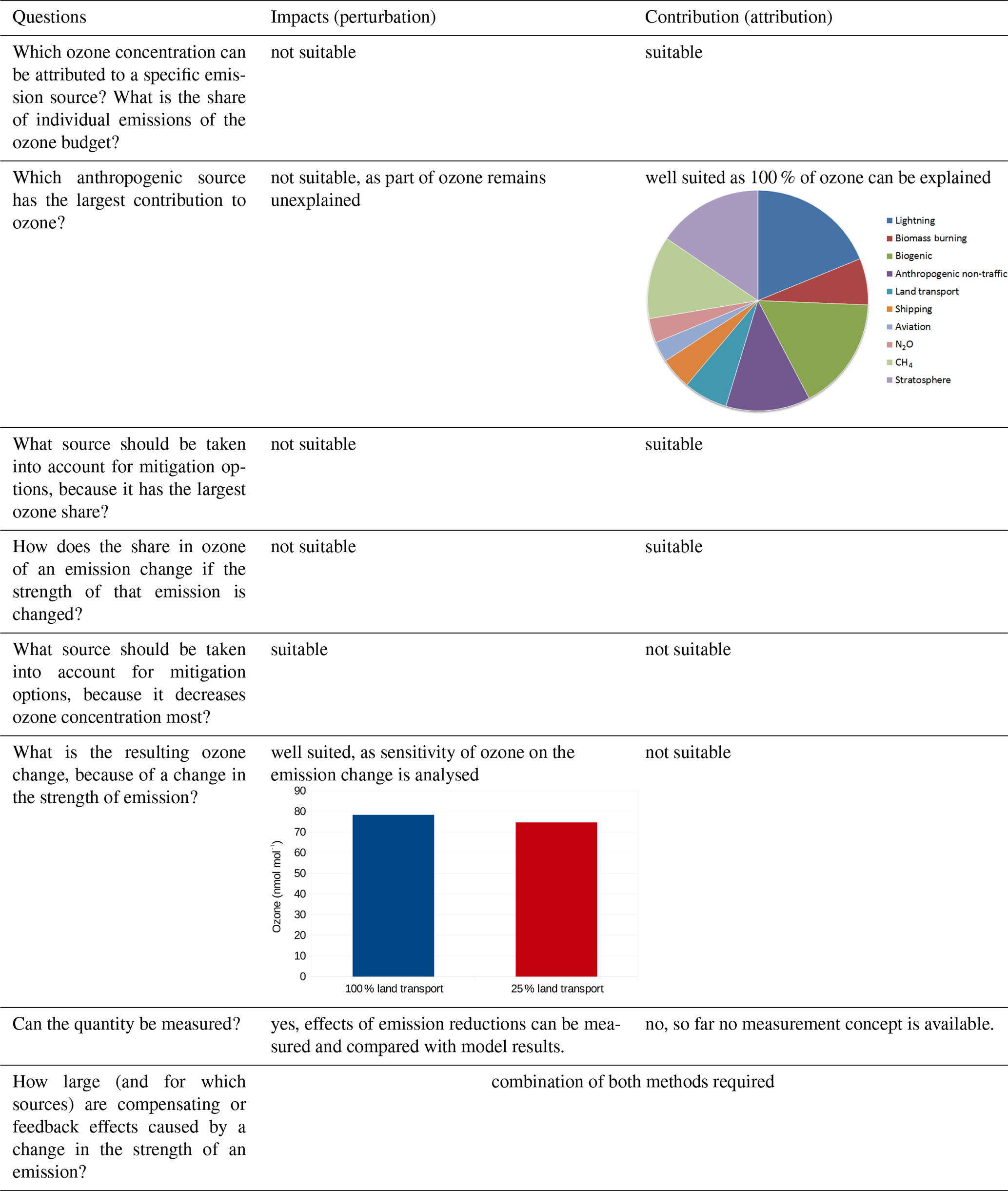
For a chemical species that is controlled by linear processes only, the perturbation method and the source attribution method lead to identical results. However, the ozone chemistry is strongly non-linear. Only for small perturbations around the base state (w.r.t. the chemical regime) can the response of ozone to a small emission change be considered almost linear. Whether a response to an emission change is nearly linear depends on the chemical regime and therefore the region and the considered time period. Thus, the perturbation approach does not allow for a complete ozone source attribution (e.g. Wild et al., 2012), because the impacts calculated for the different sectors do not sum up to 100 %. This leads to an underestimation of the contribution of specific emission sources to ozone if these impacts are used for source attribution. As an example, Emmons et al. (2012) reported that tagged ozone is 2–4 times larger than the impact calculated by the perturbation approach. Even though the difference between impact and contribution is well known in the literature, the perturbation method is still widely used for ozone attribution studies, i.e. studies in which the contributions of emission sources to the ozone budget are analysed.
In the present study we want to investigate the share of land transport emissions to European ozone levels. Therefore, we choose a source attribution method to calculate the contributions of land transport emissions to ozone and ozone precursors. The effect of mitigation options of land transport emissions is not a subject of this study. From the point of view of air quality planning, this might be seen as an academic question, but as with similar previous studies (e.g. Brandt et al., 2013; Karamchandani et al., 2017; Pay et al., 2019; Lupaşcu and Butler, 2019), our investigation improves the understanding of European ozone levels.
Many studies were performed which investigated the influence of land transport emissions to ozone on the global scale (e.g. Granier and Brasseur, 2003; Niemeier et al., 2006; Matthes et al., 2007; Hoor et al., 2009; Dahlmann et al., 2011; Mertens et al., 2018). All of them showed that land transport emissions impact ozone considerably on the global scale, especially in the Northern Hemisphere. These results of global models, however, give only very limited information on the contributions of the land transport (or other) emissions to ozone levels on the regional scale, especially as simulated ozone mixing ratios depend on the model resolution (e.g. Wild and Prather, 2006; Wild, 2007; Tie et al., 2010; Holmes et al., 2014; Markakis et al., 2015). Even though land transport is, besides other anthropogenic emissions (e.g. Matthias et al., 2010; Tagaris et al., 2014; Aulinger et al., 2016; Yan et al., 2018) and biogenic emissions (e.g. Simpson, 1995; Solmon et al., 2004; Curci et al., 2009; Sartelet et al., 2012), an important source of ozone precursors in Europe, only few studies investigated the influence of European land transport emissions on ozone. Reis et al. (2000) investigated the impact of a projected change of road traffic emissions from 1990 to 2010 on ground-level ozone in Europe, reporting a general decrease of ozone levels due to emission reductions. Similarly, Tagaris et al. (2015) quantified the impact of 10 different emission sources on European ozone and PM2.5 levels using the CMAQ (Community Multi-scale Air Quality) model for a specific period (July 2006). Tagaris et al. (2015) reported an impact of road transport emissions on the maximum 8 h ozone mixing ratio of 10 % or more in central Europe. Compared to this, Valverde et al. (2016) used a source attribution method integrated in CMAQ (Kwok et al., 2015) to investigate the contributions of road traffic emissions of Madrid and Barcelona to ozone. They reported ozone contributions of 11 % to 25 % for the Iberian Peninsula. Similarly, Karamchandani et al. (2017) applied the source attribution technique integrated in CAMx (Comprehensive Air-quality Model with extensions; Dunker et al., 2002) to calculate the contribution of 11 source categories to ozone concentrations for one summer and one winter month in 2010, focusing on 16 European cities. Generally, Karamchandani et al. (2017) reported contributions of 12 % to 35 % of the road traffic sector on the ozone levels in different cities. In accordance with other studies, Karamchandani et al. (2017) showed that European ozone levels are strongly influenced by long-range transport (e.g. Jonson et al., 2018; Pay et al., 2019). Despite the high importance of long-range transport, all discussed studies applied the source attribution method in the regional model only. Ozone and ozone precursors which are advected towards Europe (i.e. significantly influenced by boundary conditions of the regional model) are not attributed to specific emission sources (or regions) but are attributed to the boundary conditions only.
Accordingly, all of the previous studies quantified only the contribution of European land transport emissions to the European ozone levels. In contrast, the present study provides a detailed assessment on the contribution of land transport emissions to ozone and ozone precursors (NOx, CO) considering the combined effect of European and global emissions.
To include also the effects of long-range transport in regional studies, a global–regional model chain is necessary, which includes a source attribution method in the global and the regional models. Such a model is the MECO(n) model system (MESSy-fied ECHAM and COSMO models nested n times; e.g. Kerkweg and Jöckel, 2012a, b; Hofmann et al., 2012; Mertens et al., 2016), which couples the global chemistry climate model EMAC (ECHAM/MESSy Atmospheric Chemistry; e.g. Jöckel et al., 2010, 2016) at runtime to the regional chemistry model COSMO-CLM/MESSy (COSMO model in CLimate Mode with MESSy infrastructure; Kerkweg and Jöckel, 2012b). Two regional model refinements are applied, covering Europe and Germany with 50 and 12 km resolutions, respectively. The global model resolution is 300 km. The global and the regional models are equipped with the MESSy interface (Jöckel et al., 2005, 2010), and we apply the same tagging method (Grewe et al., 2017) for source attribution in the global and the regional models. Compared to previous studies, this model system allows for a contribution analysis from the global to the regional scale taking into account the effects of long-range transport (Mertens et al., 2020).
Typically, the uncertainties of such source attribution studies are large. The reasons are the following:
-
uncertainties in the models (e.g. chemical or physical parameterizations);
-
uncertainties due to the choice of source attribution methods;
-
uncertainties of the emissions inventories;
-
seasonal variability of the contributions caused by meteorological conditions and seasonal cycles of emissions (e.g. stronger biogenic emissions and more active photochemistry during summer than winter);
-
year-to-year variability of the contributions caused by meteorological conditions or large emissions of specific sources in specific years (e.g. yearly differences of biomass burning emissions).
To account for the uncertainties due to different emission inventories, simulations with two different anthropogenic emission inventories were performed. To further account for the seasonal variability, we investigate the contributions for winter and summer seasons. In addition, we consider always three simulation years to estimate the variability of the contributions between different years. The investigation of uncertainties caused by models and/or source attribution methods is beyond the scope of this study.
In our analysis we focus on mean and extreme (expressed as 95th percentile) contributions for the multi-year (2008 to 2010) seasonal average values of winter (December, January, and February, hereafter DJF) and summer conditions (June, July, and August, hereafter JJA). Our main priority is on the results of the European domain. However, as the model resolution can influence the results, we also further investigate results for the smaller domain covering Germany.
The article is structured as follows. First, Sect. 2 contains a brief description of the model system, including an introduction to the applied tagging method, a description of the performed model simulations, and the applied emission inventories, as well as a brief comparison of the simulated ozone concentrations with observations. Sections 3 and 4 discuss the contributions of land transport emissions to reactive nitrogen, carbon monoxide, and ozone in Europe. Section 5 focuses on the contribution of reactive nitrogen for Germany only based on the finer-resolved simulation results. Finally, the net ozone production over Europe and in particular the contributions of land transport emissions to the net ozone production are investigated in Sect. 6.
In this study the MECO(n) model system is applied (Kerkweg and Jöckel, 2012b; Hofmann et al., 2012; Mertens et al., 2016; Kerkweg et al., 2018). This system couples online the global chemistry–climate model EMAC (Jöckel et al., 2006, 2010) with the regional-scale chemistry–climate model COSMO-CLM/MESSy (Kerkweg and Jöckel, 2012a). COSMO-CLM is the community model of the German regional climate research community jointly further developed by the CLM-Community (Rockel et al., 2008). New boundary conditions (for dynamics, chemistry, and contributions) are provided at every time step of the driving model (e.g. EMAC or COSMO-CLM/MESSy) to the finer-resolved model instances (COSMO-CLM/MESSy). Accordingly, the MECO(n) model allows for a consistent zooming from the global scale into specific regions of interest.
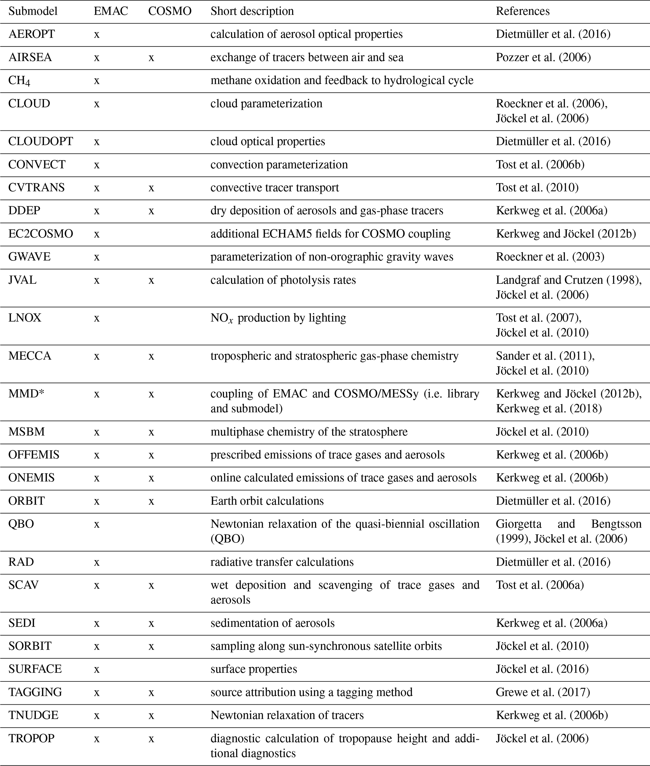
The simulations analysed in the present study are the same simulations as described in detail by Mertens et al. (2020). Therefore, we present only the most important details of the model set-up. Table 2 lists the used MESSy submodels. The global model EMAC is applied at a resolution of T42L31ECMWF, corresponding to a quadratic Gaussian grid of approx. and 31 vertical hybrid pressure levels from the surface up to 10 hPa. The time step length is set to 720 s. To achieve a higher resolution, we apply two COSMO-CLM/MESSy nesting steps. The first refinement covers Europe with a horizontal resolution of 0.44∘ and 240 s time step length, while the second refinement covers Germany with 0.11∘ horizontal resolution and 120 s time step length. Both refinements feature 40 vertical levels from the surface up to 22 km. In the following, the abbreviation CM50 (COSMO(50 km)/MESSy) corresponds to the first refinement (with roughly 50 km resolution) and CM12 (COSMO(12 km)/MESSy) corresponds to the second refinement (roughly 12 km resolution). The MESSy submodel MECCA (Module Efficiently Calculating the Chemistry of the Atmosphere; Sander et al., 2011) is applied in EMAC and COSMO-CLM/MESSy for the calculation of chemical kinetics. The chemical mechanism includes the chemistry of ozone, methane, and odd nitrogen. Alkynes and aromatics are not taken into account, but alkenes and alkanes are considered up to C4. The Mainz Isoprene Mechanism (MIM1; Pöschl et al., 2000) is applied for the chemistry of isoprene and some non-methane hydrocarbons (NMHCs). The complete namelist set-ups and the mechanisms of MECCA and SCAV (scavenging of traces gases by clouds and precipitation; Tost et al., 2006a, 2010) are part of the Supplement.
Dietmüller et al. (2016)Pozzer et al. (2006)Roeckner et al. (2006)Jöckel et al. (2006)Dietmüller et al. (2016)Tost et al. (2006b)Tost et al. (2010)Kerkweg et al. (2006a)Kerkweg and Jöckel (2012b)Roeckner et al. (2003)Landgraf and Crutzen (1998)Jöckel et al. (2006)Tost et al. (2007)Jöckel et al. (2010)Sander et al. (2011)Jöckel et al. (2010)Kerkweg and Jöckel (2012b)Kerkweg et al. (2018)Jöckel et al. (2010)Kerkweg et al. (2006b)Kerkweg et al. (2006b)Dietmüller et al. (2016)Giorgetta and Bengtsson (1999)Jöckel et al. (2006)Dietmüller et al. (2016)Tost et al. (2006a)Kerkweg et al. (2006a)Jöckel et al. (2010)Jöckel et al. (2016)Grewe et al. (2017)Kerkweg et al. (2006b)Jöckel et al. (2006)Table 2Overview of the most important MESSy submodels applied in EMAC and COSMO/MESSy. Both COSMO/MESSy instances use the same set of submodels. MMD* comprises the MMD2WAY submodel and the MMD (Multi-Model-Driver) library.
Anthropogenic, biomass burning, agricultural waste burning (AWB), and biogenic emissions are prescribed from external data sources (see Sect. 2.2). Emissions of soil NOx are calculated online (i.e. during model runtime) following the parameterization of Yienger and Levy (1995). The same applies for emissions of biogenic VOCs (volatile organic compounds), which are calculated following Guenther et al. (1995), and emissions for lightning NOx for which the parameterization of Price and Rind (1994) is applied.
The simulation period ranges from July 2007 to January 2011. The period in 2007 is the spin-up phase, and the years 2008–2010 are analysed. For reasons of computational costs, CM12 has been initialized in May 2008 from CM50 and integrated for the period May–August 2008 only. Therefore, results of CM12 are analysed for JJA 2008 only. To facilitate a one-to-one comparison with observations, EMAC is “nudged” by Newtonian relaxation of temperature, divergence, vorticity, and the logarithm of surface pressure (Jöckel et al., 2006) towards ERA-Interim (Dee et al., 2011) reanalysis data of the years 2007 to 2010. The sea surface temperature and sea ice coverage are prescribed from ERA-Interim as well. CM50 and CM12 are not nudged but forced at the lateral and top boundaries against the driving model (e.g. EMAC for CM50 and CM50 for CM12).
One feature of chemistry–climate models is the coupling between chemistry, radiation, and atmospheric dynamics, meaning that even small changes in the chemical state of the atmosphere lead to changes in the dynamics (which in turn feed back to the chemistry). This feedback can prevent a quantification of the influence of small emission changes on the atmospheric composition. To overcome this issue, Deckert et al. (2011) proposed a so-called quasi chemistry-transport model mode (QCTM mode) for EMAC, which can also be applied in MECO(n) (Mertens et al., 2016). To achieve the decoupling between dynamics and chemistry, climatologies are used within EMAC: (a) all radiatively active substances (CO2, CH4, N2O, CFC-11, and CFC-12) for the radiation calculations; (b) nitric acid for the stratospheric heterogeneous chemistry (in the submodel MSBM, Multiphase Stratospheric Box Model; Jöckel et al., 2010); and (c) OH, O1D, and Cl for methane oxidation in the stratosphere (submodel CH4). In COSMO-CLM/MESSy only the climatology of nitric acid for the submodel MSBM is required. The applied climatologies are monthly-mean values from the RC1SD-base-10a simulation described by Jöckel et al. (2016).
2.1 Tagging method for source attribution
The source attribution of ozone and ozone precursors is performed using the tagging method described in detail by Grewe et al. (2017), which is based on an accounting system following the relevant reaction pathways and applies the generalized tagging method introduced by Grewe (2013).
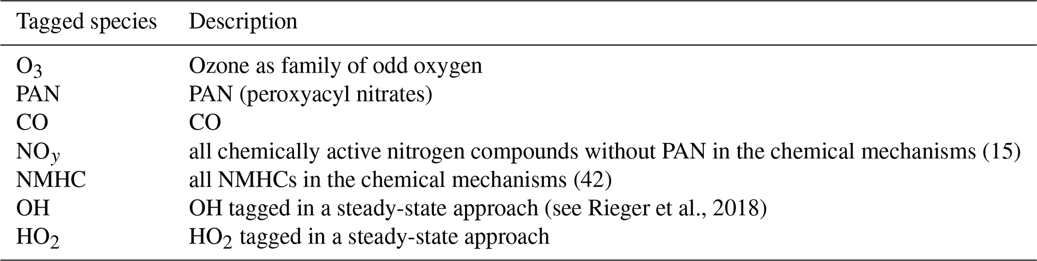
For the source attribution, the source terms, e.g. emissions, of the considered chemical species, are fully decomposed into N unique categories. The definition of the 10 categories considered in the current study are listed in Table 3. The tagging method is a diagnostic method, i.e. the atmospheric chemistry calculations are not influenced by the tagging method. To minimize the computational resources (e.g. computing time and memory consumption), the tagging is not performed for the detailed chemistry from MECCA but for a simplified family concept. The species of the family concept are listed in Table 4.
Table 3Description of the different tagging categories applied in this study following Grewe et al. (2017). Please note that some tagging categories summarize different emission sectors (see description). The last row shows the nomenclature of the tagged tracers for ozone as an example.

Table 4Definition of the chemical families used in the tagging method. More details on the species contained in the families are given in the Supplement of Grewe et al. (2017).
The production rates, loss rates, and mixing ratios of the chemical species which are required for the tagging method are obtained from the submodel MECCA. Loss processes like deposition are treated as a bulk process, meaning that the changes in the relevant mixing ratios due to dry and wet deposition are memorized and later applied to all tagged species according to their relative contributions.
Due to the full decomposition into N categories, the sum of contributions of all categories for one species equals the total mixing ratio of this species (i.e. the budget is closed):
To demonstrate the basic concept of the generalized tagging method, we consider the production of O3 by the reaction of NO with an organic peroxy radical (RO2) to NO2 and the organic oxyradical (RO):
As demonstrated by Grewe et al. (2017) (see Eqs. 13 and 14 therein), the tagging method leads to the following fractional attribution:
Here, all species marked with tag represent the quantities tagged for one specific category (e.g. land transport emissions); PR1 is the production rate of O3 by Reaction (R1); and NOy and NMHC represent the mixing ratios of the tagged families of NOy and NMHC, respectively. The denominator represents the sum of the mixing ratios over all categories of the respective tagged family or species. Accordingly, the tagging scheme takes into account the specific reaction rates from the full chemistry scheme. Further, the fractional apportionment is inherent to the applied tagging method, as due to the combinatorial approach, every regarded chemical reaction is decomposed into all possible combinations of reacting tagged species.
Some of the categories listed in Table 3 are not directly associated with emission sectors. These categories are stratosphere, CH4 and N2O. All ozone which is formed by the photolysis of oxygen, i.e.
is labelled as stratospheric ozone.
The degradation of N2O is a source for NOy (and a loss of ozone) by the reaction:
The degradation of CH4 is considered a source of . This refers to the simplified reaction
As discussed recently in detail by Butler et al. (2018), all tagging methods are based on specific assumptions and have specific limitations. The scheme by Grewe et al. (2017), which we apply in the current study, is based on specific assumptions, which differ from other tagging schemes used in regional and global models. One important difference is the question whether ozone formation is attributed to NOx or VOC precursors. The schemes which are available in the regional models CMAQ (called CMAQ-ISAM; Kwok et al., 2015) and CAMx (called CAMx OSAT; Dunker et al., 2002) use threshold conditions to check whether ozone formation is NOx or VOC limited. Depending on this, the ozone production is attributed to NOx or VOC precursors only. The scheme by Emmons et al. (2012), applied on the global scale, tags only NOx; therefore, ozone production is only attributed to NOx precursors. Based on the work by Emmons et al. (2012), Butler et al. (2018) present a scheme which attributes ozone formation to either NOx or VOCs (implying that usually two simulations, one with NOx and one with VOC tagging, are performed). This scheme was also applied by Lupaşcu and Butler (2019) in a regional model simulation over Europe, using the NOx tagging scheme only. Compared to discussed schemes, the scheme by Grewe et al. (2017) attributes ozone production always to all associated precursors (i.e. NOx, HO2 and VOCs) without any threshold conditions.
If the tagging scheme is used in addition to the perturbation approach (see Table 1) to investigate the influence of mitigation options, the approach of Grewe et al. (2017) leads to the effect that in VOC limited regions a NOx emission reduction of an emission sector reduces the contribution of that sector, and increases the contribution of the other sectors. In contrast, a reduction of VOC emissions decreases the contribution of the respective sector only. The latter is similar to the approaches integrated in CMAQ or CAMx, which attribute ozone production in the case of a VOC limit to VOC precursors only. Compared to NOx tagging, our approach leads to lower contributions of NOx sources, since they compete not only with other NOx sources but also with VOC sources.
Because of the family concept, which is necessary to keep the memory consumption and the computational costs low, the tagging method applied in our study can lead to some unphysical artefacts. As an example, Grewe et al. (2017) discuss the production of PAN (peroxyacyl nitrates) by NMHCs from CH4 degradation. Further, due to the combinatorial approach, for instance, also NMHCs from stratospheric origin can occur in small amounts, which is also an unphysical artefact. The main reason for this is the definition of the PAN family, which transfers tags from NOy to NMHCs. Other tagging schemes have specific issues as well. As an example, the scheme by Emmons et al. (2012) does not neglect the O3–NOx null cycle, which leads to an overestimation of local sources compared to long-range transport sources (see also Kwok et al., 2015). Overall, the impacts of the underlying assumptions on the results are difficult to quantify. Therefore, it is important to study effects of different emission sources with different methods (at best in the same model framework), in order to understand better the strengths and weaknesses of the different approaches and their impact on the source attribution results.
Besides these general assumptions of the different methods one specific problem occurs when applying ozone source attribution in regional models: the boundary conditions. Usually, regional studies (e.g. Li et al., 2012; Kwok et al., 2015; Valverde et al., 2016; Pay et al., 2019) just tag ozone from lateral and top boundaries as “boundary ozone”, because no boundary conditions including tagged ozone are available. Recently, Lupaşcu and Butler (2019) used results from a previous global model simulation including a NOx tagging as boundary conditions for a regional ozone source attribution study with WRF-Chem (Weather Research and Forecasting model coupled with Chemistry) over Europe. As pointed out by Mertens et al. (2020), our approach has no need for results from previous model runs, as in MECO(n) the tagging is performed in all model instances (i.e. in the global model as well as all regional model instances). Thus, consistent boundary conditions are provided for the regional model instances, and source categories for contributions from lateral or model top boundaries are not required. In the present study, the tagging method is configured such that we apply only one global tag for every source category. While this allows us to investigate the contributions of all global emissions of a specific emission source to ozone, we are not able to separate contributions from local and long-range transport. (We cannot separate contributions from, for example, European and Asian land transport emissions to European ozone levels, but we can quantify the contribution of global land transport emissions to European ozone levels.)
In the following, we denote absolute contribution of land transport emissions to ozone as . Analogously, contributions to the family of NOy and CO are denoted as and COtra, respectively (cf. abbreviations in Table 3). These absolute contributions correspond to the share of the species total mixing ratio which can be attributed to emissions of land transport. Please note that the given absolute contributions for ozone are always computed by multiplying the relative contributions to odd oxygen with the ozone mixing ratios. These values are slightly lower than the absolute contributions of odd oxygen. Besides the absolute contributions, we investigate relative contributions which give the percentage of the contribution to the total mixing ratio of the species.
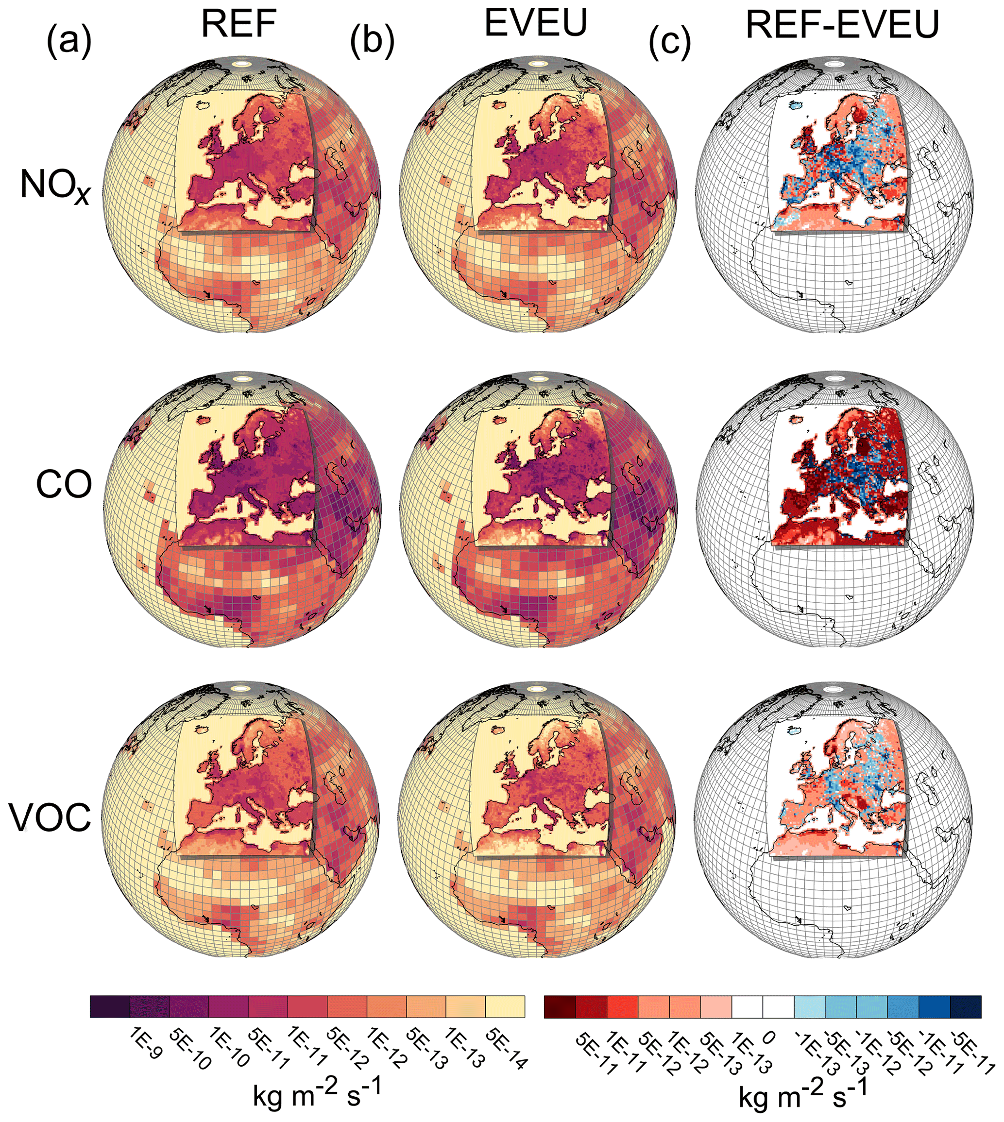
Figure 1Annually averaged emission fluxes (2008 to 2010) from the land transport sector (in ). Shown are the emissions as applied in EMAC (based on the MACCity inventory) and in CM50. The emissions of CM50 are superimposed on the emissions of EMAC. In the region covered by CM50, EMAC also uses the MACCity emissions (not visible). (a) The emissions applied in REF, (b) the emissions applied in EVEU, and (c) the difference of the emissions between REF and EVEU (“REF − EVEU”). Shown are the emission fluxes of NOx (in ), CO (in ), and VOC (in ).
2.2 Emission scenarios and numerical experiments
To investigate the influence of the uncertainties of anthropogenic emissions inventories on the source attribution results, we perform simulations for two anthropogenic emission inventories. The first emission inventory is the MACCity inventory (Granier et al., 2011), a global inventory with horizontal resolution, which corresponds to the RCP 8.5 (Representative Concentration Pathway) emission scenario for the analysed time frame (called MAC in the following). The second emission inventory is named VEU and considers emissions only for the European area ( horizontal resolution). It was composed in the DLR project “Verkehrsentwicklung und Umwelt” (VEU). For this emission inventory, the German land transport emissions were estimated bottom up by means of macroscopic traffic simulations. Finally, the land transport emissions are estimated by combining the activity data of the traffic simulations with corresponding emissions factors. For the other European countries, as well as for all other emission sectors, a top-down approach was applied. More details about the emission inventory are provided by Hendricks et al. (2017). Further details about the preprocessing of the emissions is given in Appendix A of Mertens (2017).
Two different simulations are performed:
-
REF. The MAC emission inventory is applied in EMAC and all regional refinements (e.g. CM50 and CM12).
-
EVEU. The MAC emission inventory is applied in EMAC and the VEU emission inventory in the regional refinements.
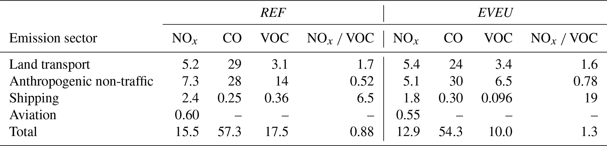
The VEU emission inventory considers only emissions for the sectors land transport, anthropogenic non-traffic (including landing and take-off (LTO) of aeroplanes), and shipping. Table 5 lists the total emissions of NOx, CO, VOC, and the ratio of NOx to VOC for these emission sectors. In general, the total emissions of the land transport sector are quite similar, while the emissions of the sectors anthropogenic non-traffic and shipping are lower in the VEU compared to the MAC emission inventory. Especially the NOx and VOC emissions are lower by around 30 % and 50 %, respectively. This leads to different NOx to VOC ratios for the total anthropogenic emissions between both emission inventories.
Table 5Average (2008 to 2010) annual total emissions for the CM50 domain of different anthropogenic emission sectors and the total of all emission sectors for NOx (in Tg(NO) a−1), CO (Tg(CO) a−1), VOC (Tg(C) a−1), and the NOx to VOC ratio (NOx ∕ VOC).
The definition of the emission sectors in VEU is different from the definition in MAC. In the VEU emission inventory LTO emissions are part of the anthropogenic non-traffic sector, but in-flight emissions from aircraft are not considered in VEU. Therefore, the MAC aviation emissions are also applied in the EVEU simulation. To avoid a double counting of the LTO emissions, the aviation emissions in MAC are set to zero in the lowermost level in EVEU, leading to a reduction of the aviation emissions of the MAC emission inventory by 0.05 Tg a−1 (see Table 5). For the emission sectors agricultural waste burning (AWB), biomass burning, lightning, and biogenic, we apply the same emissions in both simulations (see Table 6). Total emissions for the global model EMAC, and for CM12, are given in the Supplement (see Sect. S4).
Table 6Average (2008–2010) annual total emissions for the CM50 domain of NOx (in Tg(NO) a−1), CO (Tg(CO) a−1), VOC (Tg(C) a−1), and the NOx to VOC ratio (NOx ∕ VOC). Given are the total emissions of the emission sectors which are identical in REF and EVEU.
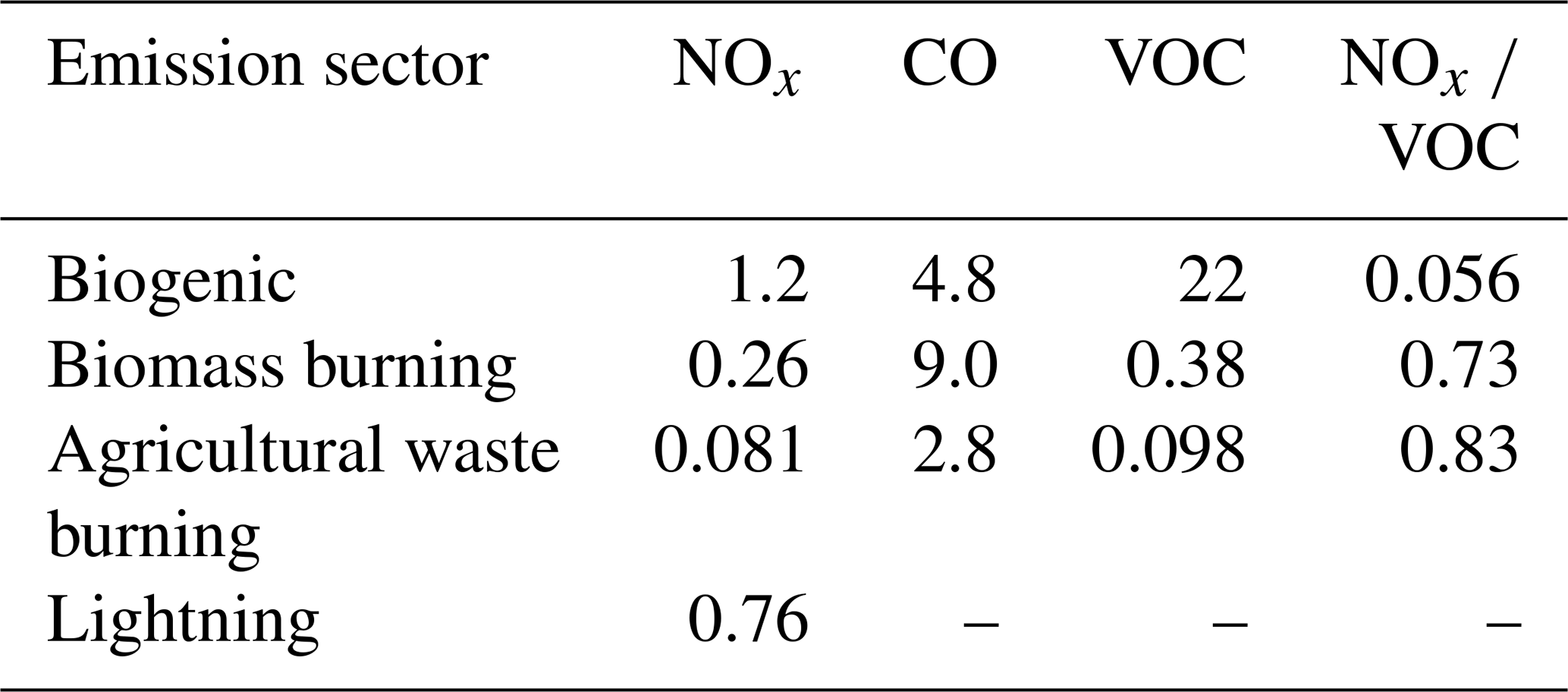
Figure 1 displays the geographical distribution of the land transport emissions of NOx, CO, and VOC applied in the REF and EVEU simulations and the emission differences between both simulations. Shown are only the emissions of EMAC and CM50, focusing on Europe. The NOx land transport emissions for CM12 are depicted in the Supplement (Fig. S7). Further, more detailed figures showing the geographical distribution in CM50 are part of the Supplement (Fig. S8). The emissions of CM50 are superimposed onto the emissions applied in EMAC, where the MACCity emissions are applied globally. Despite comparable total emissions between the MACCity and the VEU emission inventory over Europe, the geographical distributions differ. Generally, the VEU emission inventory features larger emissions near the hot-spots and lower emissions away from the hot-spots compared to MAC. Further, MAC features larger NOx emissions especially the northern part of the British Isles and in Finland. Emissions of CO are especially larger around Estonia in MAC compared to VEU. Particularly over Germany, the Po Valley, and parts of eastern Europe, VEU features more emissions of NOx, CO, and VOCs (see also totals for CM12 in Table S4). Besides the difference between the emissions applied in CM50 (and CM12), it is important to note that for the REF and the EVEU simulations the same emissions are applied in EMAC. Therefore, the difference (Fig. 1c) is zero in EMAC.

Figure 295th percentile of ozone (in µg m−3) for the period JJA 2008 to 2010 as simulated by REF (a) and EVEU (b). The background colours show the ozone concentrations as simulated by CM50, and the circles represent the location of stations of the Airbase v8 observation data. The inner point represents the measured concentrations and the outer point the concentrations in the respective grid box, where the station is located. All values are based on data every 3 h.
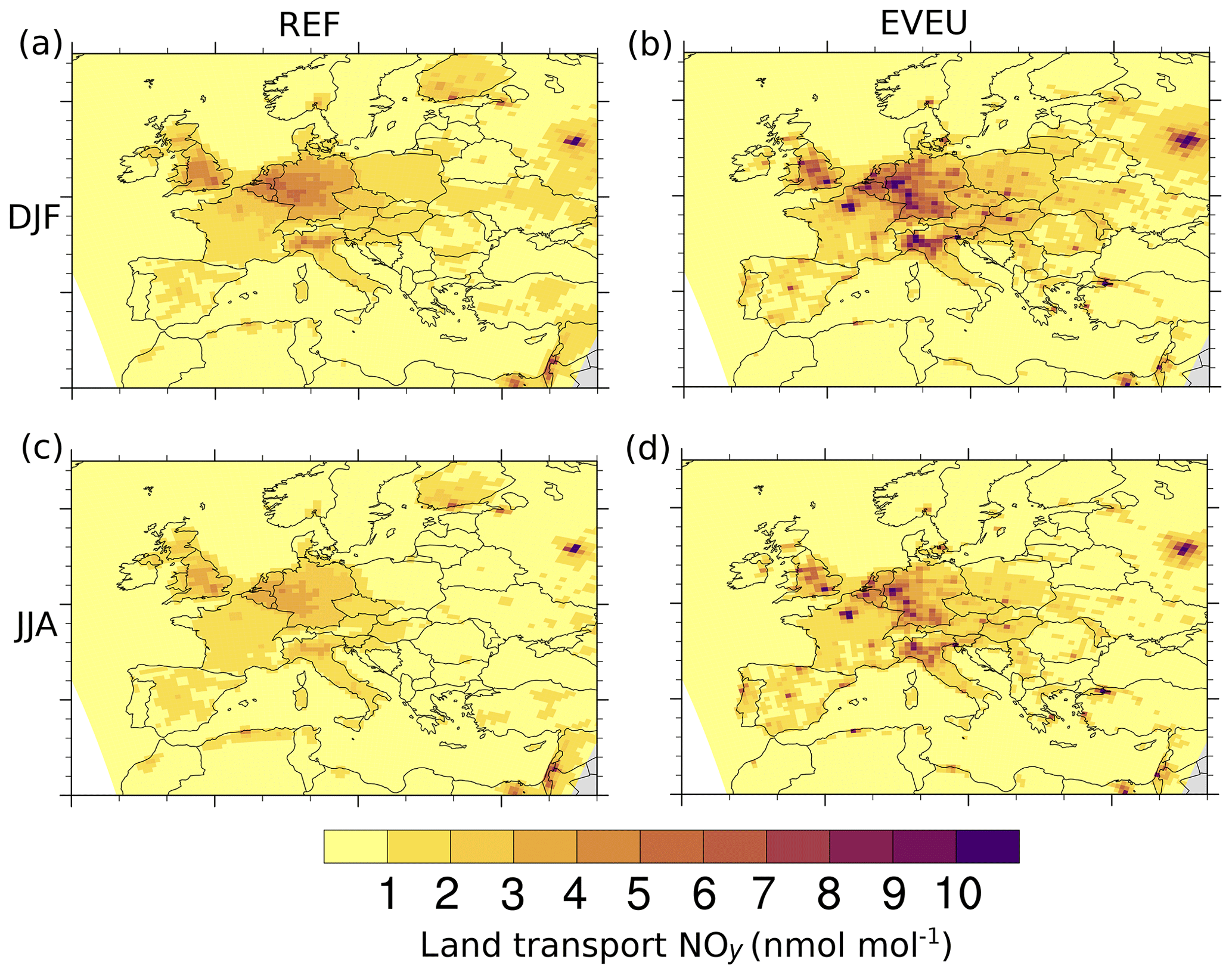
Figure 3Absolute contribution of land transport emissions to ground-level NOy (in nmol mol−1) as simulated by CM50. Panels (a) and (b) are contributions for the period DJF (2008 to 2010) of the REF and EVEU simulations, respectively. Panels (c) and (d) are contributions for the period JJA (2008 to 2010) of the REF and EVEU simulations, respectively.
2.3 Model evaluation
A model set-up very similar to the one used for the present study was evaluated with observational data by Mertens et al. (2016). Generally, the comparison showed a good agreement with observations. The biases are similar to comparable model systems and exhibit a positive ozone bias and negative biases for NO2 and CO. One important reason for these biases is the too efficient vertical mixing within the COSMO-CLM model. An evaluation of the ozone mixing ratios simulated by REF and EVEU was presented by Mertens et al. (2020) but with emphasis on JJA mean values. To investigate the model's ability to represent extreme values, we present a brief evaluation of the simulated ozone concentrations in comparison to the Airbase v8 observational dataset (https://www.eea.europa.eu/data-and-maps/data/airbase-the-european-air-quality-database-8, last access 14 February 2020). As the model resolution of 50 km is too coarse to resolve hot-spots of individual cities, we restrict the comparison to those stations which are classified as area types “suburban” and characterized as “background”. We focus on JJA 2008 to 2010 and compare the results over all 350 measurement stations. The measurements are subsampled at the same temporal resolution (3 hourly) as the model data.
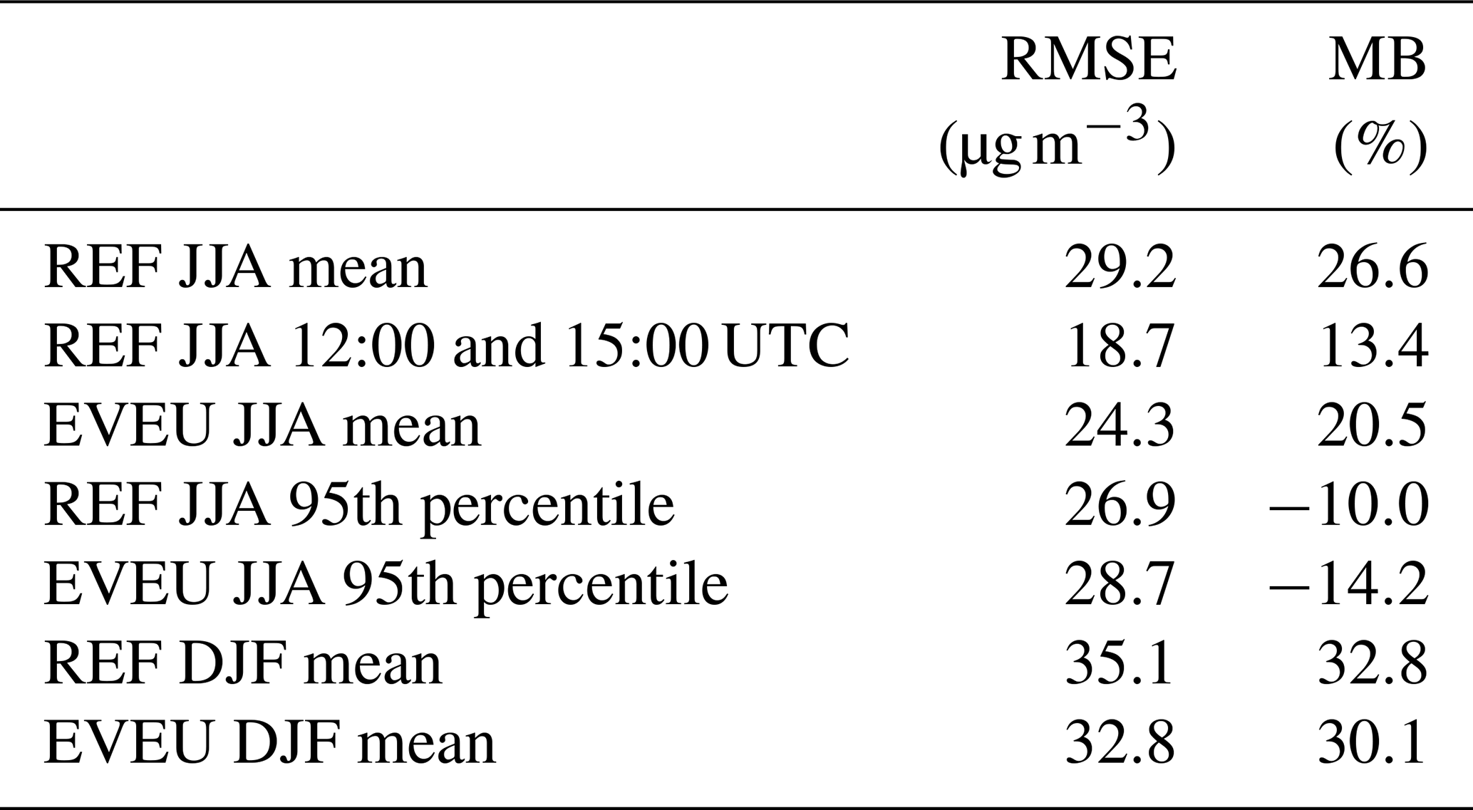
Our comparison with the Airbase v8 data shows the known positive ozone bias (Mertens et al., 2016, 2020). The average root-mean-square error (RMSE) over all 350 stations is 29.2 µg m−3 for REF and 24.3 µg m−3 for EVEU. The corresponding mean biases (MBs) are 26.6 % and 20.5 %, respectively (see Table 7). In addition, we calculated also the RMSE and MB for the REF simulation considering only measurements and model data at 12:00 and 15:00 UTC. For this subsample, both RMSE and MB decrease considerably. Accordingly, the largest ozone values during daylight are captured very well by the model. As a more detailed comparison between measurements and model result shows, the overestimation of ozone is particularly strong during night. This can partly be attributed to a too unstable boundary layer during night, which is a common difficulty in many models (Travis and Jacob, 2019). In addition, the too strong vertical mixing in the model leads to positive ozone biases at noon and during the night (see also Mertens et al., 2020, 2016). Further investigations about how this bias could be reduced in the future are currently undertaken. Besides the too efficient vertical mixing, too low ozone deposition during night, too low NO or VOC emissions, and successively underestimated ozone depletion during nights could also partly contribute to this bias.
To check the model's ability to represent extreme ozone values, the simulated 95th percentiles of ozone are compared with measurements too (see Fig. 2). Overall, the model is able to capture most of the regional variability of the extreme values over Europe. Near the densely populated regions in Benelux, Germany, and Italy, however, the model is not able to reproduce the observed 95th percentiles of ozone. In these areas the model resolutions (i.e. also for the 12 km domain, which is not shown here) are too coarse to allow for a representation of extreme ozone values in urban areas. As was shown by prior studies (e.g. Tie et al., 2010), resolutions below 10 km are required to capture large ozone values near cities. Terrenoire et al. (2015) noted that even with 8 km resolution the performance of the applied CHIMERE model is better at rural than at urban sites. This underestimation can also be quantified using the RMSEs and MBs for the 95th percentile, which are listed in Table 7.
Table 7Root-mean-square error (RMSE, in µg m−3) and mean bias (MB, in percent) of the REF and EVEU simulations compared to Airbase v8 observation data. Given are the scores for the mean values during JJA and DJF, as well as values for the 95th percentile for JJA. For REF, listed additionally, the scores considering only the values at 12:00 and 15:00 UTC are also given.
These results have important implications for the analyses presented in the present study. First of all, the too strong vertical mixing in COSMO-CLM/MESSy leads to a positive bias of the contribution of stratospheric ozone at ground level. Further, contributions of lightning and aviation at ground level are likely overestimated due to this overestimated vertical mixing. Altogether COSMO-CLM/MESSy simulates an approximately 1 percentage point lower contribution of anthropogenic emissions to ground-level ozone compared to EMAC (see Mertens et al., 2020).
Due to the coarse model resolution of 50 km, our results are representative of the regional scale, but not for specific urban areas. In these urban areas local emissions and local ozone production and destruction might be more important such that contributions of local sources can be much larger than the values we present. On the regional scale, however, Mertens et al. (2020) showed that the results are quite robust with respect to the model resolution (down to 11 km).
Because of the stronger ozone bias during night, we further compared the contributions at 12:00 and 15:00 UTC with the contributions considering all times of the day. The relative contributions show only small differences, i.e. a slightly larger contribution of anthropogenic emission sources during day (not shown). Therefore, we present always results for all times of the day.
CO and NOy are direct pollutants of the land transport sector, with different chemical lifetimes. Due to the family concept of the tagging method, we investigate contributions to NOy and not to NOx. Our focus in this section is on the results at the European scale; results of NOy for Germany will be discussed in Sect. 5. Figure 3 shows for DJF and JJA. The largest mixing ratios of are simulated near southern England, the Paris metropolitan region, western Germany, and the Benelux Union as well as the Po Valley and the Moscow metropolitan region. In these regions contributions of up to 10 nmol mol−1 are simulated. In general, larger absolute contributions occur during DJF compared to JJA, but the seasonal cycle of the land transport emissions is small in both emission inventories (see Fig. S4). Accordingly, the differences in between DJF and JJA are likely not caused by seasonal differences of the emissions but by larger mixing layer heights and a more effective photochemistry during JJA compared to DJF.
The seasonal change in is smaller than differences between REF and EVEU. Near areas with large land transport emissions, EVEU simulates 3 to 4 nmol mol−1 larger contributions than REF. In most of the hot-spot regions (e.g. Paris and the Po Valley) the differences are even larger and the contributions calculated by EVEU are 5 nmol mol−1 larger than in REF. In some regions the results of both simulations are in total contrast. In REF for example, absolute contributions of up to 4 nmol mol−1 are simulated in Finland, while EVEU simulates absolute contributions below 1 nmol mol−1.
The relative contribution of land transport emissions to ground-level NOy is in the range of 40 % to 70 % in most parts of Europe (see Fig. 4). These relative contributions are similar to the share of land transport NOx emissions to all NOx emissions (see Fig. S9), but compared to the share of the emissions, the contributions to NOy are slightly lower near hot-spots and larger in rural areas.
During DJF, REF simulates the lowest relative contributions of 30 % to 50 % over most parts of Europe. During summer the contributions increase up to 60 % with the largest values in southern Germany, the Po Valley, and southern England. EVEU simulates a smaller difference of the contributions between DJF and JJA as REF. Further, the maxima are generally slightly larger and contributions of up to 70 % are simulated around the Po Valley and the Paris area. Interestingly, the relative contributions are lower during DJF than during JJA, while the absolute contributions are larger during DJF than during JJA. Most likely this is caused by the lower amount of anthropogenic non-traffic NOx emissions during JJA compared to DJF (see Fig. S4).
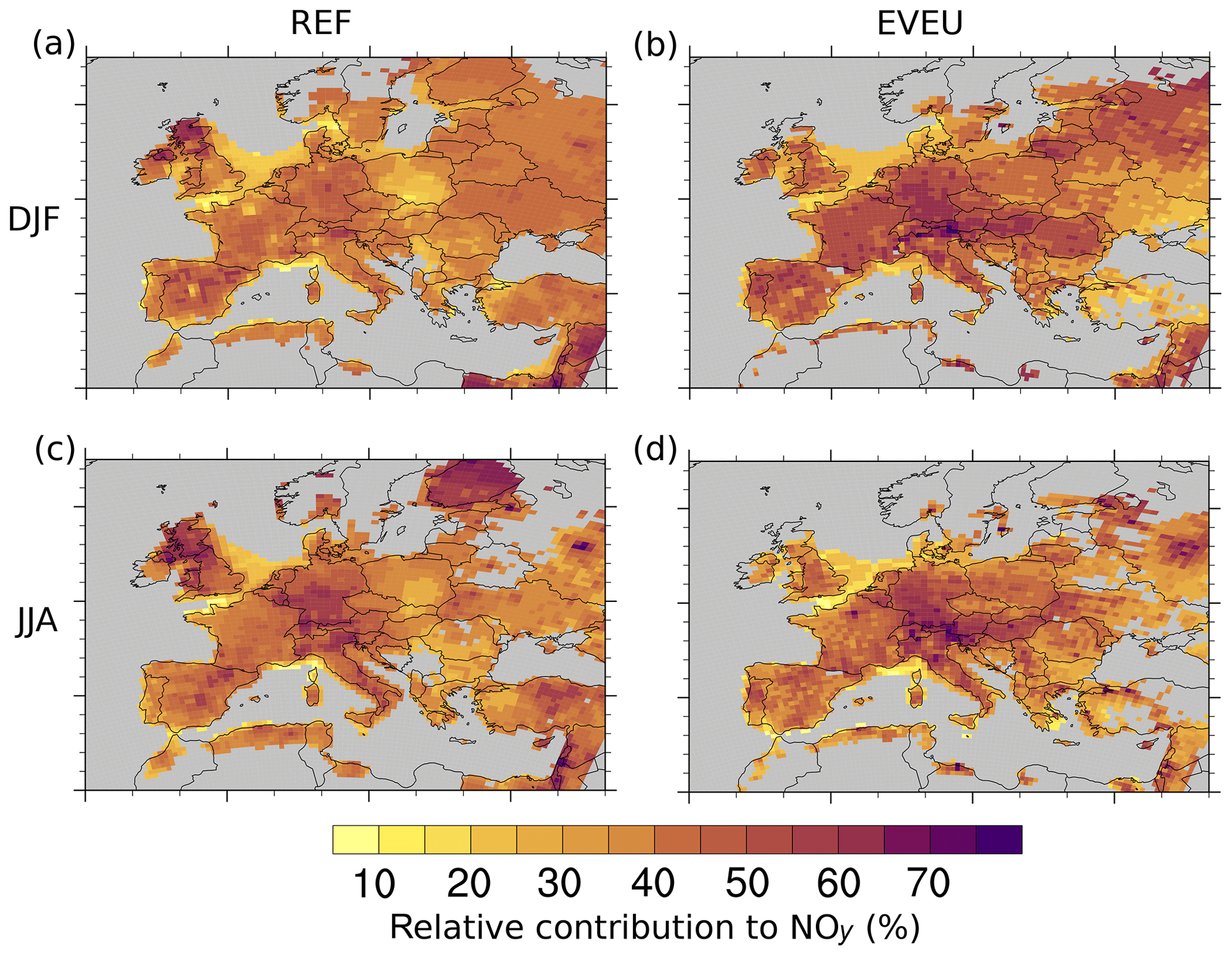
Figure 4Relative contribution of land transport emissions to ground-level NOy (in percent) as simulated by CM50. Panels (a) and (b) are contributions for the period DJF of the REF and EVEU simulations, respectively. Panels (c) and (d) are contributions for the period JJA of the REF and EVEU simulations, respectively. Grey areas indicate regions where the absolute NOy mixing ratios are below 0.5 nmol mol−1. In these regions no relative contributions are calculated for numerical reasons.
The simulated mixing ratios of COtra (see Fig. 5) show a similar behaviour as , implying that contributions in DJF are larger than in JJA. This seasonal difference is most likely caused by lower mixing layer heights and increased lifetime of CO during DJF compared to JJA, as OH concentrations are lower in winter compared to summer. Generally, the largest contributions are simulated in southern England, around Paris, western Germany, the Po Valley, and around Moscow. In EVEU contributions of up to 75 nmol mol−1 are simulated around London, Paris, Milan, and Moscow, while the results of the REF simulation show lower contributions in the western European regions of mostly 50 to 60 nmol mol−1. Compared to , however, some hot-spots stand out in the results of the two simulations. EVEU, for example, shows larger contributions (40 to 60 nmol mol−1) to CO over Hungary or southern Poland. Contrary to this, REF shows contributions of 30 to 50 nmol mol−1 over Estonia. These differences between contributions are directly attributable to the differences in the emission inventories (Fig. 1). Hence, the uncertainties with respect to the CO emissions of land transport in these regions are quite large.

Figure 5Absolute contribution of land transport emissions to ground-level CO (in nmol mol−1) as simulated by CM50. Panels (a) and (b) are contributions for the period DJF of the REF and EVEU simulations, respectively. Panels (c) and (d) are contributions for the period JJA of the REF and EVEU simulations, respectively.
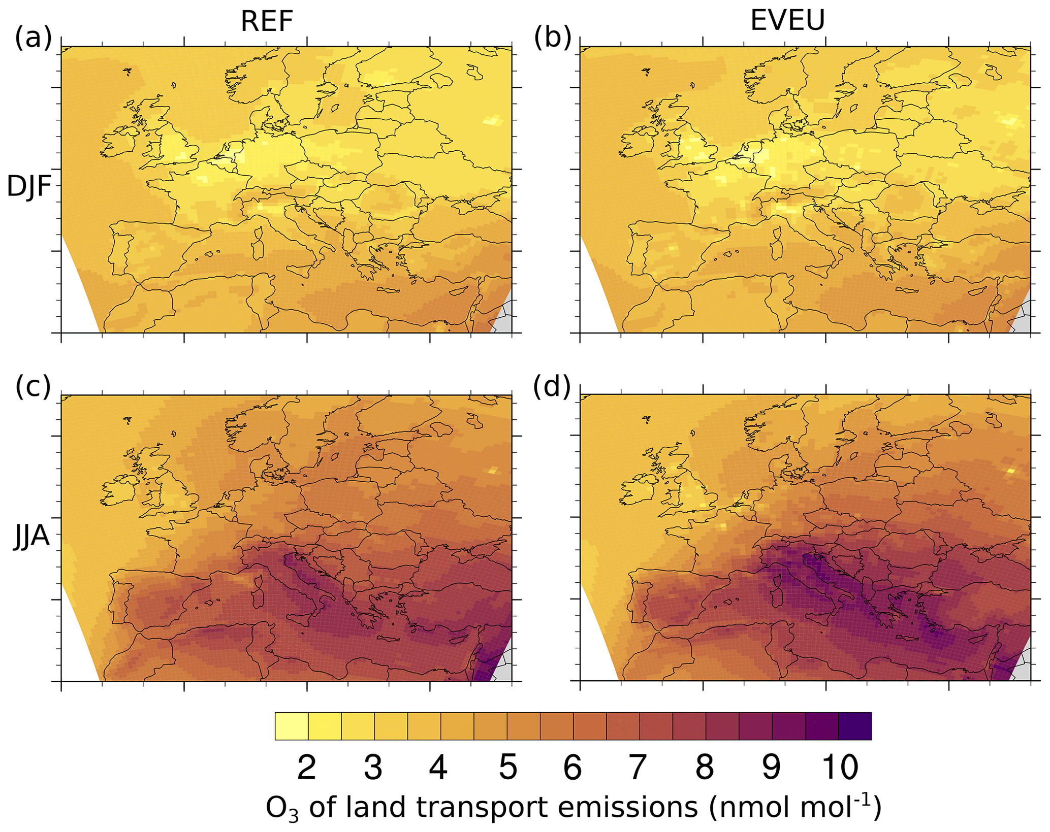
Figure 6Absolute contribution of land transport emissions to ground-level O3 (in nmol mol−1) as simulated by CM50. Panels (a) and (b) are contributions for the period DJF of the REF and EVEU simulations, respectively. Panels (c) and (d) are contributions for the period JJA of the REF and EVEU simulations, respectively.
In contrast to NOy and CO, ozone is a secondary pollutant and emissions have an indirect effect on it. Therefore, this section quantifies the contribution of land transport emissions to ozone in detail. Besides land transport emissions, however, many other sources contribute to ground-level ozone. Generally, the most important sources which contribute globally to ozone are downward transport from the stratosphere, anthropogenic non-traffic, shipping, lightning, and biogenic emissions (e.g. Lelieveld and Dentener, 2000; Grewe, 2004; Hoor et al., 2009; Dahlmann et al., 2011; Emmons et al., 2012; Grewe et al., 2017; Butler et al., 2018). Table 8 lists the contributions of different emission sources to ozone for Europe averaged for JJA 2008 to 2010 and for the results of EVEU and REF (see also Fig. S6 for zonally averaged vertical profiles of the contributions). The most important sources for ground-level ozone in Europe are biogenic emissions (≈19 %), anthropogenic non-traffic emissions (≈16 %), methane degradation (≈14 %), and land transport emissions (≈12 %). With increasing height, the contributions of ground-based emission sources decrease; accordingly, the contribution of land transport emissions decreases to ≈8 % at 600 hPa. At the same time the importance of ozone transported downward from the stratosphere, lightning, and aviation increases. At a height of 200 hPa more than 50 % of the ozone is from stratospheric origin. The contribution of land transport emissions drops to around 3 %. Further, the differences between the results of REF and EVEU decrease with increasing height, indicating the larger importance of long-range transport. The latter is equal in both simulations due to identical emissions for the global model and therefore identical boundary conditions for CM50 for the global model.
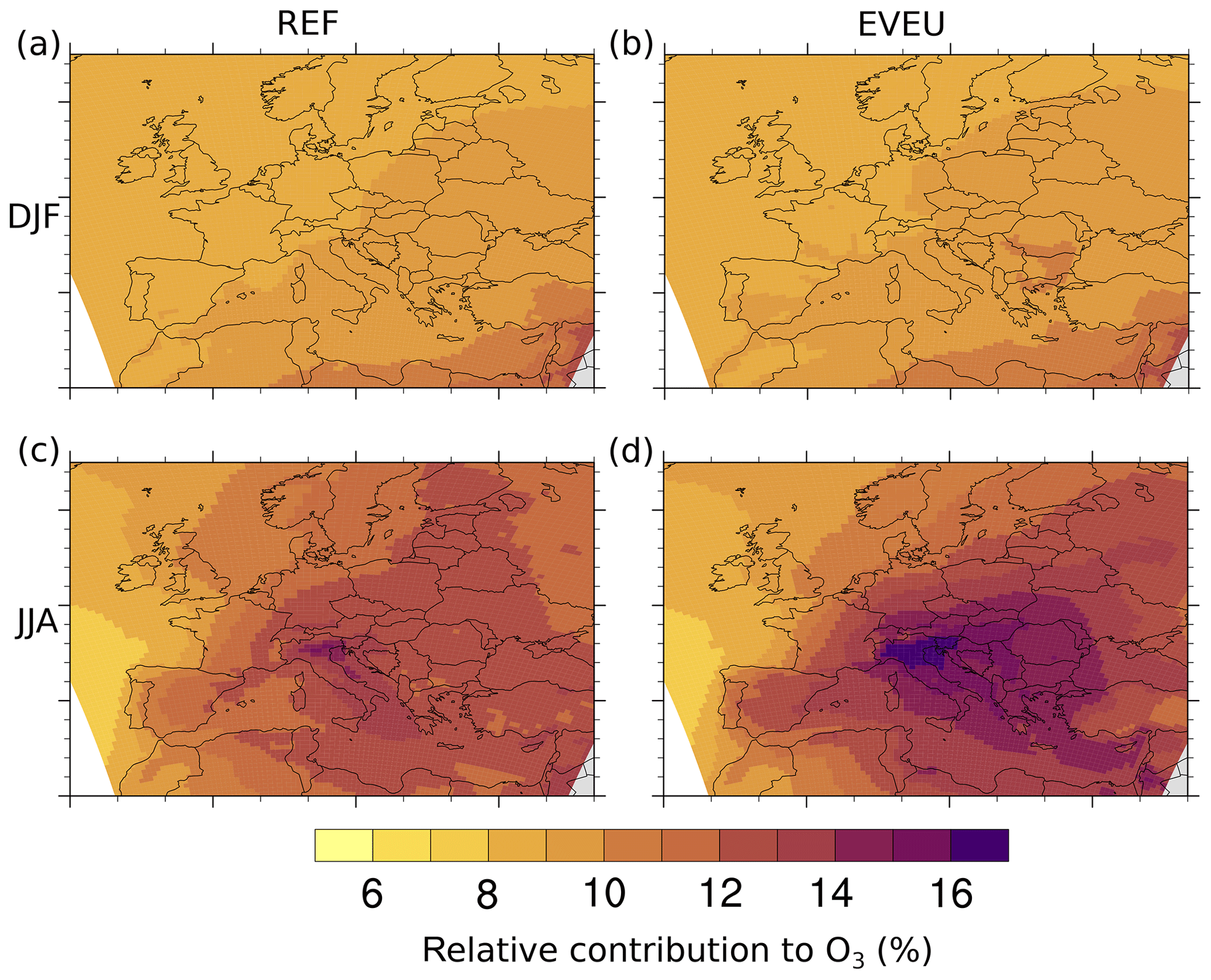
Figure 7Relative contribution of land transport emissions to ground-level O3 (in percent) as simulated by CM50. Panels (a) and (b) are contributions for the period DJF of the REF and EVEU simulations, respectively. Panels (c) and (d) are contributions for the period JJA of the REF and EVEU simulations, respectively.
Table 8Area-averaged contribution of different emission sources over Europe (defined as a rectangular box 10∘ W to 38∘ E and 30 to 70∘ N) for JJA 2008–2010 at three different altitudes (in percent). The values are mean values of the REF and EVEU simulations: the range indicates the standard deviation between the results of REF and EVEU.

4.1 Seasonal average contribution to ground-level ozone
DJF ground-level simulated by REF and EVEU (see Fig. 6) ranges between 2 and 4 nmol mol−1. Even lower ground-level is simulated near some hot-spots due to ozone titration. The absolute contributions mentioned above correspond to relative contributions of of around 8 % over large parts of Europe (see Fig. 7). Although the European emission inventories differ in the simulations, the contributions (absolute and relative) show almost no differences. The emissions of the global model, however, are identical in REF and EVEU, leading to identical contributions at the boundaries of the regional domain. Hence, the contributions during DJF are mainly dominated by long-range transport towards Europe which was reported by Karamchandani et al. (2017). This is caused by the low ozone production and long lifetime of ozone during winter.
During JJA the ozone production increases and local emissions play a larger role. Therefore, increases to 5 to 10 nmol mol−1, implying an increase of the contributions to 10 % to 16 %. The geographical distribution of the contribution is similar for both emission inventories, showing increasing absolute and relative contributions from north-west to south-east. The largest relative contributions are simulated around the Po Valley, while the largest absolute contributions are shifted downwind from Italy to the Adriatic Sea. In these regions the differences between the results of the two simulations are largest, reaching up to 2 nmol mol−1 for the absolute and 2 percentage points for the relative contributions. The larger differences between the results of REF and EVEU during summer compared to winter are mainly caused by the increasing ozone production over Europe during spring and summer. Accordingly, differences in the emission inventories modify the regional ozone budgets more efficiently.
To quantify the contributions of land transport emissions and other emission sources in different regions in more detail, Fig. 8 shows area-averaged relative contributions for JJA and DJF for the REF and EVEU simulations (absolute contributions are given in Tables S1 to S8). The geographical regions were defined according to the definitions of the PRUDENCE project (Christensen et al., 2007). However, we performed some slight modifications. The Alps region was split up into two separate regions called “Northern Alps”, defined as a rectangular box (46∘ to 48∘ N and 9∘ to 13∘ E), and “Po Valley” (44∘ to 46∘ N and 5 to 15∘ E). Note, however, that the region Northern Alps contains parts of Switzerland and southern Germany, which are still rather flat and subject to large land transport emissions. In addition, we defined a region called inflow (40∘ to 60∘ N and 11∘ to 13∘ W). This region is used to quantify contributions in the air advected towards Europe. A figure summarizing the definition of all regions is part of the Supplement (Fig. S12).
The relative contribution of in the inflow region is about 9 % in both seasons and for both European emission inventories. During DJF the contributions in all regions are very similar. During JJA the contribution of land transport emissions increases in most regions compared to the inflow (≈9 %). In the Po Valley reaches up to 16 %. Unfortunately, the difference between in a specific region and in the corresponding region inflow cannot be used to calculate from European emissions. Such a calculation requires different tags for global and European land transport emissions. The relative contribution of other anthropogenic emissions (anthropogenic non-traffic, shipping, and aviation; see also Table 3) in the inflow region (≈34 %) is also very similar in both seasons. During DJF the contributions over all regions in Europe are very similar to the contribution in the inflow region. During JJA, in contrast, a west–east gradient of the anthropogenic contributions is present over Europe with a decrease down to ≈27 % in eastern Europe. This decrease is mainly due to the seasonality of the different emissions (discussed further below). The biogenic emissions category shows different relative contributions in the inflow region during DJF (≈11 %) compared to JJA (≈14 %). This is mainly caused by the strong increase in biogenic emissions during summer compared to winter. In the different regions the relative contributions increase during JJA compared to DJF, and, compared to the inflow by up to ≈20 %. The contribution of all other tagging categories during DJF is ≈47 % in most regions, and it ranges between 41 % and 36 % during JJA.
As already discussed, the emissions of the land transport sector show almost no seasonal cycle (Fig. S4), while the absolute and relative contributions of show a seasonal cycle. This seasonal cycle is caused by a complex interplay of the seasonal cycles of different emission sources, meteorology, and photochemical activity. The seasonal cycle of the relative contribution of is shown in Fig. 9. The seasonal cycle of the absolute contribution is similar to the cycle of the relative contribution but shows the largest peak during June when the absolute ozone levels are largest (see Fig. S10). The contribution peaks between May and July and in October (≈13 % averaged over Europe for the column up to 850 hPa), and it has a minimum of 9 % during December to March. The decrease of the contribution during the summer months is mainly caused by the large contribution of biogenic emissions (biogenic VOCs and soil NOx) during July and August and subsequent increasing contributions of . The decrease of the contribution during DJF is mainly caused by increasing contributions from the stratosphere and anthropogenic non-traffic emissions. The categories show a strong seasonal cycle with peaks of the contributions during March and May (Fig. S3). The indicated standard deviation of the contribution shows that in winter, spring, and autumn the year-to-year variability (blue shading) is the most important source of uncertainty. Here, differences in regional emissions lead only to small differences (orange shading). During summer, however, the differences of the regional emissions strongly contribute to the uncertainties.
The differences between the extreme absolute and relative contributions of between REF and EVEU (expressed as 95th percentile) are larger than for the mean values. The 95th percentile of the relative contribution of to ground-level ozone reaches up to 24 % in the Po Valley using the VEU emission inventory (see Fig. 10). In REF the maxima are lower by 4 to 5 percentage points compared to EVEU. In contrast to the mean values, the extreme values occur mainly near the regions with the largest land transport emissions, namely over France, Italy, and Germany. Over France and Germany extreme values (depending on the applied emission inventory) in the range of 16 % to 18 % occur, while the values in northern Italy range from 20 % to 24 %.
Focussing on Germany, the relative contribution of to ground-level ozone is 10 % to 15 %. The contribution has a north-west-to-south-east gradient. One important contributor to this gradient is the strong shipping emissions in the English Channel, North Sea, and Baltic Sea (e.g. Matthias et al., 2010). These emissions lead to larger relative and absolute contributions of shipping emissions in northern and western Germany, which decrease towards the south. The absolute contributions are around 2 to 3 nmol mol−1 during DJF and 4 to 6 nmol mol−1 during JJA (averaged for 2008 to 2010). The largest 95th percentile of the relative contribution of land transport emissions is simulated in southern Germany (up to 22 %).

Figure 8Area-averaged relative contributions to ground-level ozone (in percent) in different geographical regions for DJF 2008 to 2010 (triangles) and JJA 2008 to 2010 (squares). Shown are the results of the REF (blue) and the EVEU simulations (red) for (a) the land transport category, (b) the anthropogenic emissions, (c) the biogenic category, and (d) all other categories. For simplicity, the anthropogenic category contains the anthropogenic non-traffic, aviation, and shipping categories. The residual contains all other categories. The vertical-axis scale differs from (a) to (d).
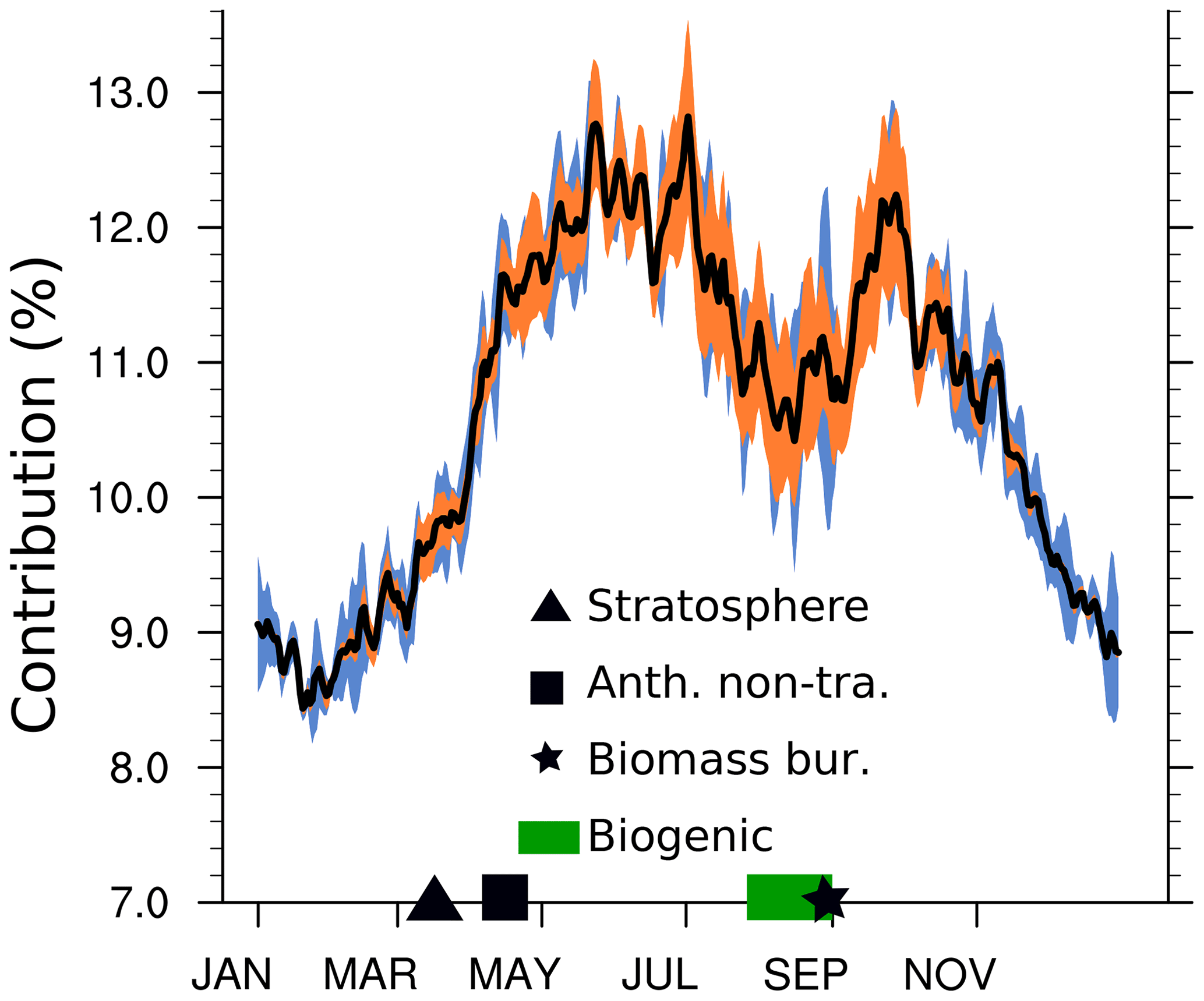
Figure 9Seasonal cycle of the relative contribution of to the ozone column up to 850 hPa (in percent). The black line indicates the mean contribution as simulated by CM50, averaged over the years 2008–2010 and the two simulations (REF, EVEU). The blue shading indicates the standard deviation with respect to time for the years 2008 to 2010 for the EVEU simulation. The orange shading indicates the standard deviation with respect to time between the 2008–2010 averaged seasonal cycles of the REF and the EVEU simulations. The symbols on the horizontal axis indicate the time frames during which the categories named stratosphere, anthropogenic non-traffic (anth. non-tra.), biomass burning (biomass bur.), and biogenic contribute the most.
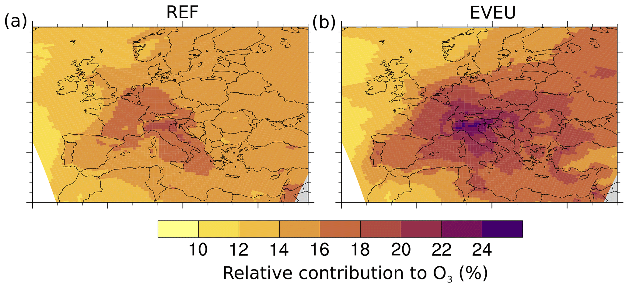
Figure 1095th percentile of the relative contribution of (in percent) as simulated by CM50 based on 3-hourly model output. Panels (a) and (b) are contributions for JJA of the REF and EVEU simulations, respectively.
4.2 Contribution during extreme ozone events
To better characterize episodes of extreme ozone values, it is important to know which emission sources contribute to and/or drive these extreme ozone values. Therefore, we investigate the contribution of land transport emissions during extreme ozone episodes. As discussed in Sect. 2.3 the contributions we report are representative of the regional scale. For analyses of the local scale (i.e. individual cities), the resolution of the model is too coarse.
First, the 99th, 95th, and 75th percentiles of the ozone mixing ratios for the period JJA 2008 to 2010 are calculated (based on 3-hourly model output; see Figs. S1 and S2). Second, the categories contributing to these 99th, 95th and 75th percentiles of ozone are analysed. Generally, the contributions to these extreme values have a high spatial variability. To capture this spatial variability, the contributions are analysed for the whole CM50 domain as well as for specific regional subdomains as introduced in Sect 4.1.
The range of contributions in the different regions is shown in Fig. 11. Generally, the relative contribution of (Fig. 11a and b) increases for increasing ozone percentiles in most regions. This increase is largest in the following regions: Po Valley, Northern Alps, mid Europe, France, and the British Isles. The largest contributions of occur in the Mediterranean region, Northern Alps, Po Valley, mid Europe, and France. Especially in these regions, EVEU simulates larger median and maximum relative contributions of compared to REF. Further, the range of contributions for almost all regions is larger in EVEU compared to REF. The ozone values at the 95th percentile (see Sect. 2.3) and at the other percentiles (see Figs. S1 and S2), however, are similar for REF and EVEU (i.e. none of the emission inventories lead to strongly different representations of extreme ozone events in the model). Accordingly, the discussed differences of the relative contributions are not caused by a different representation of the ozone values themselves but only due to the different geographical and sectoral distributions of the emissions in REF and EVEU. This demonstrates the large uncertainty, especially for contributions analysed for episodes with large ozone values of the source attribution analyses which is caused by the uncertainties of emissions inventories (e.g. geographical distribution of emissions, total emissions per sector). These uncertainties must be taken into account in source attribution studies focusing on periods with extreme ozone values.
For the 99th percentile of ground-level ozone, the median of the relative contributions of in the region Po Valley is around 17 %∕22 % (REF ∕ EVEU simulation), while the 95th percentile is around 18 %∕25 %. The contributions in the region Northern Alps are only slightly smaller, as parts of southern Germany and Switzerland with large land transport emissions are also part of this region. The region with the third largest contributions is mid Europe (including mainly Germany and the Benelux Union). Here, median contributions (at 99th percentile of ozone) of 16 %∕18 % and contributions (at 95th percentile) of 18 %∕23 % are simulated. The largest contributions (between 24 and 28 % for the EVEU simulation) are mainly simulated in the Po Valley, in south-western Germany, western Germany, and around Paris. For the lower percentiles of ground-level ozone, the contribution of land transport emissions decreases and reaches median contributions of 13 % to 16 % and 95th percentiles of 15 % to 21 % in the regions Mediterranean, Northern Alps, mid Europe, and France.
The medians of the relative contribution of other anthropogenic emissions (i.e. the emission sectors anthropogenic non-traffic and aviation) range in all regions from 17 % to 25 % (Fig. 11c and d). Hence, the contribution of other anthropogenic emissions is larger than the contribution of land transport emissions. The increase in the contribution of other anthropogenic emissions with increasing ozone percentiles, however, is lower compared to the increase of . Accordingly, the relative importance of land transport emissions increases with increasing ozone values, and hence land transport emissions are an important driver of large ozone values. This is in general in line with Valverde et al. (2016), who found that concentration peaks of ozone in Barcelona and Madrid can be explained by ozone attributed to road transport emissions. However, their contributions are in general much larger than the contributions we found (see more details in Sect. 7). Besides the contribution of land transport emissions, however, also the relative contribution of biogenic emissions to ozone increases with increasing ozone levels (Fig. 11e and f). Therefore, also biogenic emissions play an important role during episodes with large ozone values.
While the relative contributions to ozone of the shown categories increase with increasing ozone levels, the contribution of the shipping emissions and all other categories decreases with increasing ozone levels in almost all regions (Fig. S5). Only in the Mediterranean region does REF simulate a small increase of the relative contribution of shipping emissions with increasing ozone levels.
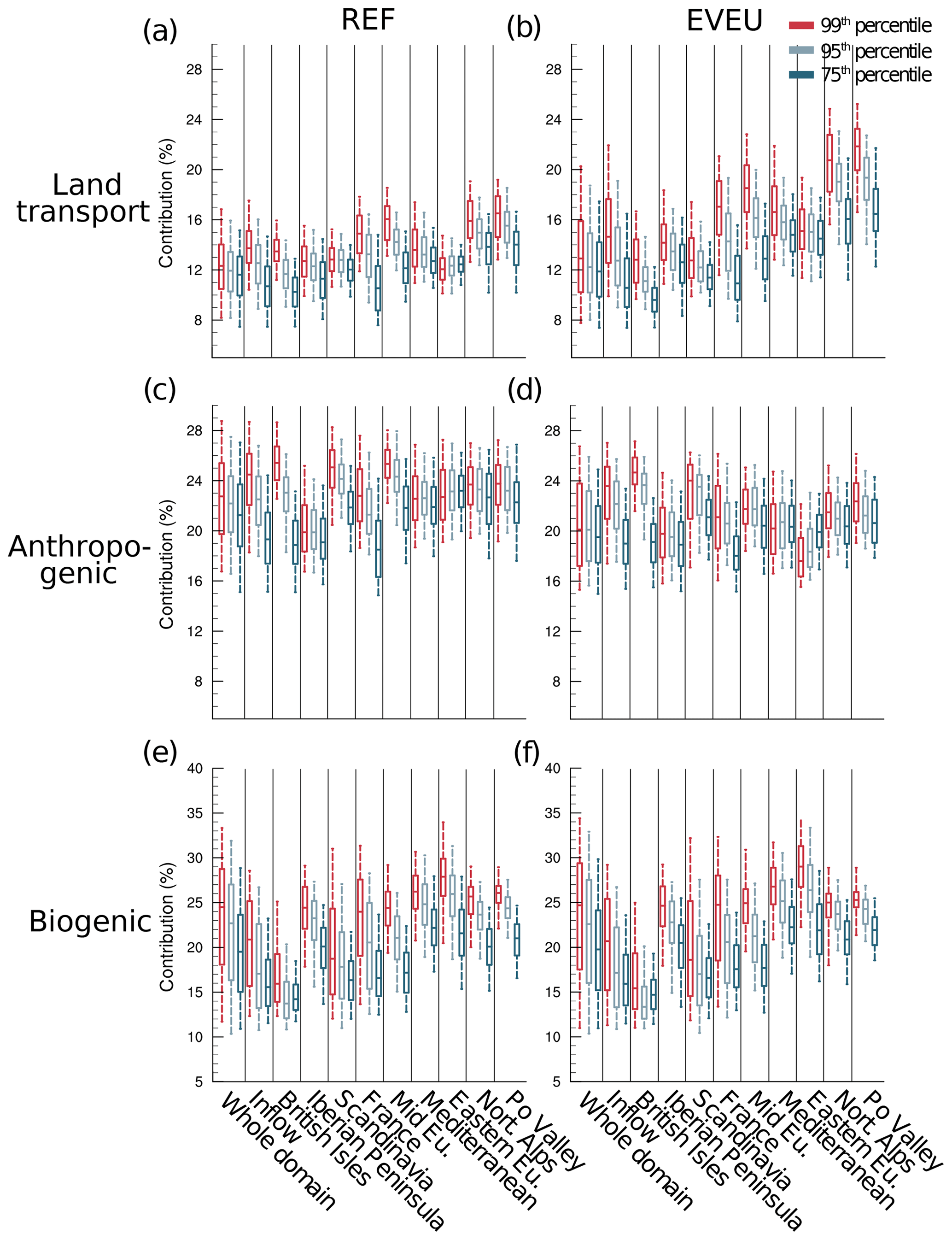
Figure 11Box-whisker plot showing the contributions of the most important emission sources at the 99th, 95th, and 75th percentiles of ozone as simulated by CM50. For simplicity, only the contributions for land transport, biogenic, and other anthropogenic emissions (anthropogenic non-traffic and aviation) to ground-level ozone (in percent) are shown. Therefore, the contributions do not add up to 100 %. Panels (a) and (b) show the relative contribution of ; (c) and (d) the relative contribution of anthropogenic emissions (anthropogenic non-traffic and aviation); and (e) and (f) the relative contribution of . The lower and upper end of the box indicate the 25th and 75th percentile, the bar the median, and the whiskers the 5th and 95th percentile of the contributions of all grid boxes within the indicated region. All values are calculated for JJA of the period 2008 to 2010 and are based on 3-hourly model output. The data are transformed on a regular grid with a resolution of to allow for the regional analyses.
So far the results of the European domain are analysed. The resolution of the VEU emission inventory, however, is much finer (roughly 7 km) as the resolution of the European domain. Accordingly, the full potential of the emission inventory is not revealed. Therefore, this section is dedicated to the results of CM12 focusing on Germany. As shown by Mertens et al. (2020) the contribution of land transport emissions to ozone in Germany changes only slightly, when the model resolution is increased from 50 to 12 km. The changes due to the increase in the resolution are smaller than the differences between the results of both emission inventories. Therefore, we focus on the contribution of land transport emissions to NOy, where the results depend stronger on the model resolution. The results of for Germany are discussed at the end of Sect. 4.1.
Figure 12 shows the absolute contribution of for JJA 2008 as simulated by CM12. As already discussed, the differences between the two emission inventories are rather large. The REF simulation shows maximum contributions of around 5 nmol mol−1, while the EVEU simulation shows contributions of up to 12 nmol mol−1. These large values occur around the large cities in Bavaria (Munich, Nuremberg) and the large cities in (south-)western Germany (Stuttgart, Frankfurt, Rhine-Ruhr area). These results indicate the importance of land transport emissions for the mixing ratios of reactive nitrogen levels in German cities. Further, they clearly show the importance of finely resolved emission inventories (and models) for source attribution of short-lived chemical species.
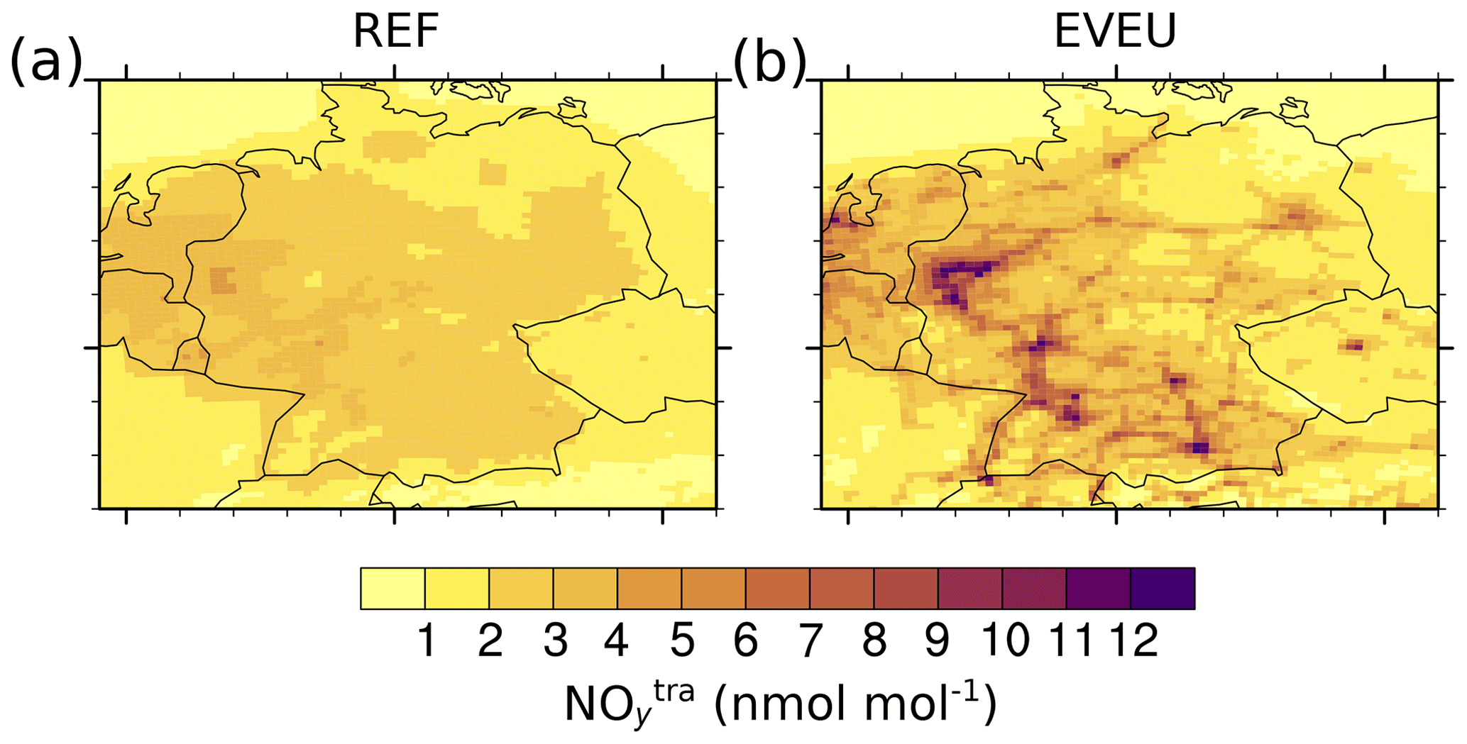
Figure 12Absolute contribution of NOytra (in nmol mol−1) for JJA 2008 of land transport emissions as simulated by CM12. Panels (a) and (b) show contributions for the period JJA of the REF and EVEU simulations, respectively.
We analyse the contribution of land transport emissions to the ozone budget in Europe by investigating the net ozone production, which is defined as
with production (ProdO3) and loss rates (LossO3) of ozone as diagnosed by the tagging method for the different tagged categories (see Sect. S5).
According to the analysis (see Table 9) the land transport emissions are the second most important anthropogenic emission sector contributing to in Europe. In general, the results obtained with both emission inventories are rather similar, caused by similar total emissions of the land transport sector. For both simulations, due to land transport emissions integrated over the CM50 domain and up to 850 hPa is around 13 Tg(O3) a−1. integrated up to 200 hPa is 23 Tg(O3) a−1.
Table 9Diagnosed net ozone production () of the 10 considered categories (in Tg a−1) as simulated by CM50. The production rates are integrated over the CM50 domain and up to 850∕200 hPa, respectively. The values are averaged for 2008–2010, and the ranges indicate one standard deviation with respect to time based on the annual averages of the individual years.

The differences between contributions of discussed in Sect. 4 are mainly caused by the differences of the total emissions of the anthropogenic non-traffic sector. of the anthropogenic non-traffic category differs by roughly 30 % between REF and EVEU, whereas the total net ozone production differs by roughly 15 %. Due to the lower total emissions in the VEU emission inventory compared to the MAC inventory, less ozone is produced in the former.
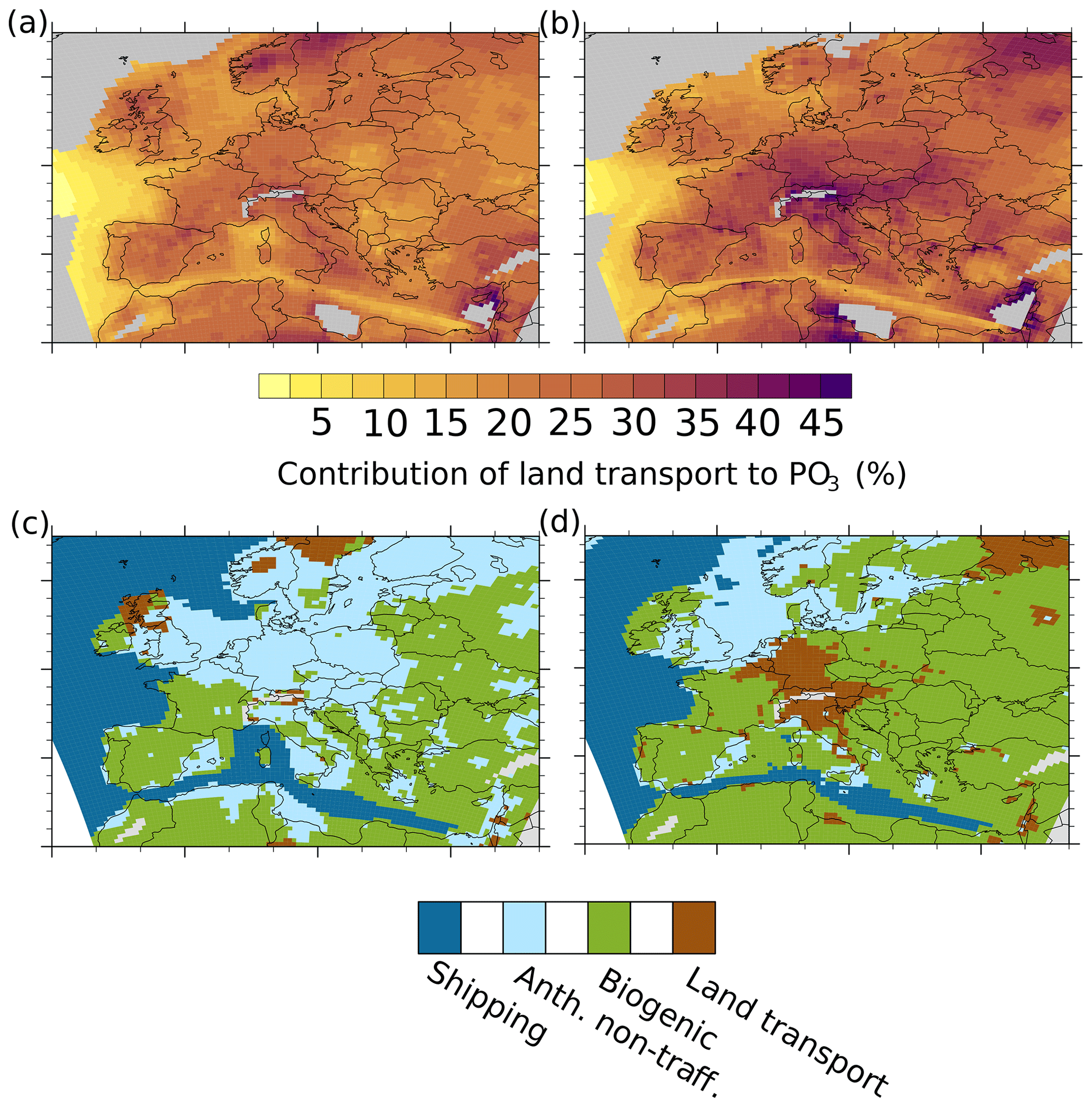
Figure 13Contribution analysis for integrated from the surface up to 850 hPa. Panels (a) and (b) show the relative contribution of land transport emissions to (in percent) for the REF and the EVEU simulations, respectively. Panels (c) and (d) indicate the emission sectors which contribute most to up to 850 hPa for the REF and EVEU simulations, respectively. Averaged data for the period May–September 2008 to 2010 as simulated by CM50 are analysed. Grey areas in (a) and (b) indicate regions where is below . In these regions no relative contributions are calculated for numerical reasons.
The regions where ozone is predominantly formed by land transport emissions are displayed in Fig. 13a and b, showing the relative contribution of land transport emissions to . Here, the analysis is restricted to the period May to September where is largest. Additionally, Fig. 13c and d indicate the emission sectors which contribute most to up to 850 hPa in the respective grid box. Consistent with previous analyses, the results show that the relative contribution of land transport emissions to is in general larger in EVEU compared to REF. The contribution is lowest over the Atlantic and along the main shipping routes in the Mediterranean Sea. In these regions ozone up to 850 hPa is mainly formed from shipping emissions (Fig. 13c and d). Generally, the contribution of land transport emissions to is largest over central Europe, including parts of the Iberian Peninsula, the British Isles, and Italy. In these regions the contributions range from 25 % to 35 % in REF and 25 % to 40 % in EVEU. Further, the regions of large contributions extend much more to the east (including Austria and Hungry) in EVEU compared to REF. Besides these regions, the contributions of land transport emissions to range from 15 % to 20 % in most areas. However, both simulation results indicate regions, especially in northern Europe but also in the Mediterranean Sea and Africa, with very large contributions (above 35 %). These regions, however, generally show low absolute values of . Therefore, the large contribution of land transport emissions is not very meaningful.
With contributions from 25 % to 40 %, land transport emissions contribute significantly to the ozone production up to 850 hPa. However, in only very few regions (western Germany, Austria, and northern Italy) and only in EVEU land transport emissions are the most important contributors to (Fig. 13).
Outside these regions the results of REF and EVEU show that biogenic emissions are most important over the Iberian Peninsula, large parts of eastern Europe, and Africa. For central Europe and northern Europe, the REF results indicate that the anthropogenic non-traffic category is most important, while the EVEU results indicate biogenic and land transport as the most important. This underlines that the uncertainty of such analysis is strongly influenced by the uncertainties of the anthropogenic and biogenic emissions inventories (or parameterizations to calculate these emissions).
Our analyses demonstrate the importance of land transport emissions to European reactive nitrogen (NOy) mixing ratios. The largest contribution of land transport emissions to NOy are simulated in southern England, Benelux, Rhine-Ruhr, Paris, and the Po Valley. These regions correspond well with the regions where ground-level measurements, satellite observations, or air quality simulations report the largest nitrogen dioxide levels (e.g. Curier et al., 2014; Vinken et al., 2014b; Terrenoire et al., 2015; Geddes et al., 2016; European Environment Agency, 2018). While the absolute contributions in these regions depend strongly on the emission inventory (5 to 10 nmol mol−1), the relative values are generally 50 % and more. Accordingly, land transport emissions are one of the most important contributors to NOy in regions with large NO2 concentrations.
These large amounts of NOx emissions from land transport clearly contribute to the formation of ozone, but the relative contributions to ozone are lower than the contributions to NOy. Here, the mean contributions range between 10 % and 16 % in most regions and even during extreme ozone events the contributions are below 30 %. Clearly, land transport emissions are an important contributor to European ozone levels but they are not the most important contributor. This is underlined by our analysis of the contribution of land transport emissions to ozone production in Europe, which range from 20 % to 40 % in most areas. The emission sectors which are most important for ozone production in Europe are biogenic emissions and anthropogenic non-traffic emissions. During periods of large ozone values, however, our analyses show that the contribution of land transport emissions to ozone increases strongly, while the contribution of anthropogenic non-traffic emissions is only slightly changed. This suggests that emissions from land transport make an important contribution to large ozone values.
We find that the regions with the largest contribution of land transport emissions to ozone are not necessarily identical with the regions with the largest contributions to reactive nitrogen. The ozone values peak mainly in northern Italy (around the Po Valley) and southern Germany, which is consistent with the findings of Tagaris et al. (2015). For the Po Valley in particular, ground-level measurements show that this is one of the regions with the largest ozone levels in Europe (e.g. Martilli et al., 2002; Guerreiro et al., 2014; European Environment Agency, 2018). In southern England, around Paris, Benelux, and the Rhine-Ruhr region, where the contribution of land transport emissions to NOy stands out the contributions to ozone are not the largest. The result, that regions are hot-spots for NOy from land transport emissions but not for O3 from land transport is counter-intuitive. The reason for this is that large amounts of NOx emissions alone are not sufficient for large ozone production. This is caused by the non-linearity of the ozone chemistry, including the availability of VOCs, and the strong interdependence of ozone production and meteorological conditions (e.g. Monks et al., 2015).
A detailed comparison of our results with previous studies is complicated. First, we apply one global tag for the land transport sector and do not differentiate between local-produced ozone and long-range-transported ozone. In comparison to our approach, similar regional studies usually attribute ozone only to the emissions within the regional domain and attribute long-range transported ozone to the boundary conditions. Second, the methods for source apportionment applied in various studies differ. Third, the applied emission inventories differ and so do ozone metrics and simulated periods. Tagaris et al. (2015), who calculated the impact of different emission sectors on ozone using a 100 % perturbation of the respective emission sectors, reported an impact of European road transport emissions of 7 % on average for the maximum 8 h ozone values in July 2006. In most regions impacts above 10 % were reported, with maximum local impacts (southern Germany, northern Italy) of above 20%. While their largest impacts occur in similar regions as our largest contributions (southern Germany, northern Italy), our mean contributions are larger than their impacts, but the maximum contributions are lower than their maximum impacts. Further, around London and in parts of northern England, their impacts (see Fig. 3 therein) are around 2 % to 4 %, while our contributions are in the range of 8 % to 10 %. Hence, impact and contribution differ largely in these regions. This is in line with previous work stating that for ozone source attribution contributions instead of impacts should be used (Grewe et al., 2012, 2019).
All the studies that we are aware of and which reported contributions of land transport emissions to ozone over Europe using a tagging method either applied the CAMx model (CAMx OSAT method; Karamchandani et al., 2017) or the CMAQ model (CMAQ-ISAM method; Valverde et al., 2016; Pay et al., 2019). As discussed, these two methods examine proxies of the ozone sensitivity to determine whether ozone production is NOx or VOC limited. These previous studies considered only European emissions, while we consider the combined effect of European emissions and long-range transport. Therefore, one would expect that our contribution analysis shows larger contributions compared to previous studies. However, our contributions in general are lower compared to previously reported values. As an example, Karamchandani et al. (2017) reported contributions around larger European cities in the range of 11 % to 24 % and in Budapest even up to 35 %. Valverde et al. (2016) reported contributions of road transport emissions from Madrid and Barcelona of up to 24 % and 8 %, respectively. Similarly, Pay et al. (2019) diagnosed contributions of road transport emissions on ozone of 9 % over the Mediterranean Sea and up to 18 % over the Iberian Peninsula but for a specific summer episode only (July 2012). To discuss potential reasons why our contributions are lower compared to previous estimates, we analysed our results for July 2010 to compare these contributions directly with the findings of Karamchandani et al. (2017).
As an example, Karamchandani et al. (2017) reported contributions of 17 % around Berlin, while our contributions are in the range of 12 %–14 %. Further they diagnosed contributions from the biogenic sector of around 11 % around Berlin, while we find contributions of the biogenic sector of around 18 %. Generally, the contributions reported by Karamchandani et al. (2017) seem to be much more variable over Europe compared to our results. A reason for this might be the different treatment in the attribution of NOx and VOC precursors. Land transport emissions contribute mainly to NOx emissions, while biogenic emissions are an important source of VOCs. As shown by Butler et al. (2018), anthropogenic emissions contribute most to ozone over Europe if a NOx tagging is applied, while biogenic emissions are the most important contributor when VOC tagging is applied (Figs. 3 and 4 therein). Accordingly, those approaches which use a threshold to perform either a VOC or NOx tagging attribute ozone production under VOC limitation mainly to biogenic sources, while under a NOx limitation ozone is attributed mainly to anthropogenic sources (including land transport emissions). Most likely this leads to a much stronger variability between anthropogenic and biogenic contributions compared to our approach, where ozone is always attributed to NOx and VOC or HOx precursors.
Similar effects can also be observed when comparing our results to the results of Lupaşcu and Butler (2019), who applied a NOx tagging for the period April to September 2010 and considered regional as well as global sources similar to our approach. They reported contributions of biogenic emissions in Europe for the period July–September between 5 % and 13 % over Europe. Our results show contributions of biogenic emissions which are much larger (15 % to 26 % for the same period). In their approach, ozone is only attributed to biogenic NOx emissions, while we attribute ozone to biogenic NOx and VOC emissions. In addition, our estimated stratospheric contribution to ground-level ozone is larger than the contributions reported by Lupaşcu and Butler (2019). Our results indicate stratospheric contributions for July to September in the range of 5 % to 10 % compared to their 2 % to 4 %. Similarly, for lightning NOx our model shows larger contributions (6 %–12 %) compared to the 3 %–6 % diagnosed by Lupaşcu and Butler (2019).
The differences in the contributions for the stratospheric and the lightning category can partly be attributed to the more efficient vertical mixing in COSMO-CLM. Mertens et al. (2020) reported a maximum difference of the contributions from the stratosphere and lightning to ozone between EMAC and COSMO-CLM/MESSy of 30 %. The difference between our results for lightning and stratospheric contributions and the results of Lupaşcu and Butler (2019) are much larger as this 30 %. Therefore, the difference can most likely not be fully attributed to differences in vertical mixing. Rather, the differences can probably be explained by the different contributions of the biogenic category (due to different tagging methods) and by differences in lightning emissions and the treatment of stratospheric ozone.
In general, the various studies discussed above do not provide sufficient information on the emissions parameterizations and inventories used (e.g. for lightning NOx, soil NOx, and biogenic VOCs) to fully analyse these differences. The discrepancy in the results of the different source attribution methods clearly shows that a coordinated comparison between these methods is important. This was already suggested by Butler et al. (2018).
The comparison of the results between the two emission inventories sheds light on the uncertainties associated with such a source attribution method. The differences in the results for the direct pollutants CO and NOy are rather large. The mean ozone contributions are much less influenced than the direct pollutants. Especially during winter and in the middle-to-upper troposphere, the contributions are mainly dominated by long-range transport (e.g. land transport emissions from the rest of the world). In our study, however, we focused only on the uncertainties caused by different emission inventories for Europe. Therefore, we did not investigate the influence of uncertainties from emissions from the rest of the world. Uncertainties in these emissions are likely to influence the contribution from long-range transport.
The results based on the two emission inventories show only small differences between the mean ozone values but large differences between the corresponding extreme ozone values and net ozone production rates, even though the total land transport emissions between the two emission inventories are similar. These differences are mainly due to the differences between the anthropogenic non-traffic emissions and the shipping emissions between the two emission inventories. Accordingly, the source attribution of land transport emissions is not only influenced by the uncertainties of the land transport emissions but also by the uncertainties of all other emission sectors. Further, it is also likely that emission inventories underestimate land transport emissions. As an example, Kuik et al. (2018) reported an underestimation of road traffic emissions for Berlin by up to 50 %. The impact of such large underestimations on the source attribution results needs to be investigated. Besides uncertainties in anthropogenic emissions, uncertainties in biogenic emissions also contribute to uncertainties of the source attribution results. In this context uncertainties in biogenic VOC emissions and NOx emissions from soil especially play an important role. As an example, the uncertainties of soil NOx are rather large (Vinken et al., 2014a) and the emissions applied in our model system are at the lower end of current emission estimates. Similar large uncertainties are also reported for biogenic VOC emission inventories (Ashworth et al., 2010; Han et al., 2013; Oderbolz et al., 2013).
Generally, uncertainties caused by the emissions are larger than the uncertainties which are caused by the simplifications applied in our source attribution method, which are of the order of some percent (see also discussion by Mertens et al., 2018). Further, our results indicate a large seasonal variability of the contribution of land transport emissions to ozone. This variability is not only caused by the meteorological conditions but also by the seasonal cycle of other emissions. Accordingly, not only the total emissions of different emission sectors but also their seasonality (and the correct representation of this seasonality) plays an important role.
The question of how to evaluate these source attribution results also remains a challenge. Clearly, a comparison of different source attribution methods would help in revealing individual strengths and weaknesses of the methods. In addition, measurements of specific episodes or in specific regions (e.g. in plumes of cities, in regions with strong lightning activity, or events of stratospheric intrusions) can help to assess the diagnosed contributions by investigating if these contributions are in a plausible range. Further, the influence of model biases on the analysed contributions can be estimated, but a direct evaluation of these contributions is not possible. However, the diagnostic information from the source attribution methods can help to understand the modelled ozone production in more detail and can offer important insights to understand potential model biases.
In the present study we investigate the contributions of land transport emissions to pollutants in Europe and Germany by focusing on ozone (O3), carbon monoxide (CO), and reactive nitrogen (NOy) by means of simulations with the MECO(n) model system. This model system couples a global chemistry–climate model online with a regional chemistry–climate model. To quantify the contributions of land transport emissions to these species, we used a tagging method for source attribution. This tagging method is an accounting system which completely decomposes the budgets of ozone and ozone precursors into contributions from different emission sources. For the first time, such a method is applied consistently in the global as well as the regional models to attribute ozone and ozone precursors to the emissions of land transport. To consider the uncertainties associated with the emission inventories, we performed simulations with two different emission inventories for Europe.
The contribution of land transport emissions to ground-level NOy depends strongly on the applied emission inventory. In general the contributions range from 5 to 10 nmol mol−1 near the European hot-spot regions, which are western and southern Germany, the Po Valley, southern England, and the Paris and Moscow metropolitan regions. In most other parts in central and southern Europe, contributions of around 2 to 3 nmol mol−1 are simulated. Generally, absolute contributions during winter are larger than during summer, but the seasonal differences are smaller than the differences between different emission inventories. The absolute contributions correspond to relative contributions of 50 % to 70 % to ground-level NOy, which indicates that land transport emissions are one of the most important sources for NOy near ground level.
Similarly to NOy the simulated contribution of land transport emissions to CO near ground level depends strongly on the applied emission inventory. Generally, the contributions range around 30 nmol mol−1 during summer in regions which are not directly associated with large land transport emission sources and more than 75 nmol mol−1 near emission hot-spots such as Paris or Moscow.
The contribution of land transport emissions to ozone, which is a secondary pollutant, shows a geographical distribution which differs strongly from the distribution of the primary emissions. The absolute contribution shows a strong north-west-to-south-east gradient with the largest contributions around the Mediterranean Sea. Due to the non-linear behaviour of ozone chemistry and the strong dependency of ozone formation on meteorology and other precursors such as NOx (mainly CO, CH4, and VOCs), regions with large emissions in western Europe (Benelux, British Isles, western Germany) show no peak of the contribution of land transport emissions to ozone. Such a peak is simulated in the Po Valley, where large emissions and favourable conditions for ozone production prevail. Generally, the contribution has a strong seasonal cycle with values of 2 to 3 nmol mol−1 during winter and 5 to 10 nmol mol−1 during summer. These absolute contributions correspond to relative contributions in the range of 8 % to 16 %. During winter, the results obtained for the two European emission inventories show almost no differences. The contributions are largely determined by long-range transport and the year-to-year variability is the largest source of uncertainty. Of course, also the uncertainties in the emission inventories for emissions outside of Europe can influence the contribution analyses noticeably, but this has not been investigated in the present study. During summer the differences between the contributions diagnosed using the two emission inventories are larger than the year-to-year variability. Hence, during summer uncertainties of emissions inventories for Europe influence the contribution analyses considerably.
While the emissions of the land transport sector have almost no seasonal cycle, the contributions exhibit a strong seasonal cycle. This shows the strong influence of seasonal cycles of other emission sources on the ozone production from land transport emissions. Hence, uncertainties in total emissions, geographical distributions, and the seasonal cycles of other emissions strongly influence the contribution analysis of land transport emissions. Especially during summer biogenic emissions play a key role here. The impact of uncertainties in these emissions needs to be studied in more detail. In addition, the impact of the applied source attribution method needs to be investigated in a coordinated way. Our results suggest that our methodology, which accounts for NOx and VOCs at the same time, leads to a partitioning between anthropogenic and biogenic sources partly different from previous studies which account for either NOx or VOCs.
The contribution of land transport emissions to extreme (99th percentile) ozone values is largest in the Po Valley, reaching up to roughly 28 %. In other regions of Europe the contribution of land transport emissions to extreme ozone events is lower and strongly depends on the region and the emission inventory. It is important, however, that the contribution of land transport emissions to ozone increases with increasing ozone levels. This indicates that land transport emissions play an important role for ozone production during episodes with large ozone values. Generally, the contribution of land transport emissions to ozone production up to 850 hPa is around 20 % and 40 % in most European regions. However, only in very few regions are land transport emissions the most important contributor to ozone production. In most regions anthropogenic non-traffic and biogenic emissions are more important. Our analysis shows that the biogenic emissions are also especially important during episodes with large ozone values. Their contribution increases with increasing ozone levels similar to the contribution of land transport emissions. The contribution of anthropogenic non-traffic emissions shows almost no increase. However, the large differences obtained for the two emission inventories indicate a large uncertainty range for such an analysis.
As discussed in our introduction (see Table 1), contributions provide the share of ozone caused by specific emissions. With respect to mitigation options, it is important to point out that these contributions provide no information about how ozone changes if the corresponding emission sources are reduced. As discussed, this question can only be assessed with the perturbation approach. However, the contributions indicate how important different emission sources are for the tropospheric ozone budget in Europe.
As a next step the analysis will be refined using source attribution categories, which differentiates between contributions of European land transport emissions and land transport emissions from the rest of the world. Such an analysis will help to quantify the importance of European and global land transport emissions to ozone levels in Europe. Further, more reliable emission estimates are important for follow-up studies. Here, the focus should not only be on the land transport emissions, but also on other important emissions, especially including biogenic VOCs and soil-NOx emissions, which are subject to large uncertainties and contribute strongly to European ozone levels. To better constrain the uncertainties of the contribution analysis, follow-up studies are planned (see Sect. 7) in which we will combine observational data of specific aircraft measurement campaigns together with model results including the analysed contributions.
The Modular Earth Submodel System (MESSy) is continuously developed and applied by a consortium of institutions. The usage of MESSy and access to the source code is licensed to all affiliates of institutions which are members of the MESSy Consortium. Institutions can become a member of the MESSy Consortium by signing the MESSy Memorandum of Understanding. More information, including how to become a licensee for the required third-party software, can be found on the MESSy Consortium website (http://www.messy-interface.org, last access: 26 June 2020). The simulations have been performed with a release of MESSy based on version 2.50. All changes are available in the official release (version 2.51). The namelist set-up used for the simulations is part of the Supplement. The model data used in this study are available under the following DOI: https://doi.org/10.5281/zenodo.3908469 (Mertens, 2020).
The supplement related to this article is available online at: https://doi.org/10.5194/acp-20-7843-2020-supplement.
MM performed the simulations, analysed the data, and drafted the manuscript. AK and PJ developed the model system. VG developed the tagging method. RS drafted the study. All authors contributed to the interpretation of the results and to the text.
The authors declare that they have no competing interests.
This article is part of the special issue “The Modular Earth Submodel System (MESSy) (ACP/GMD inter-journal SI)”. It is not associated with a conference.
We acknowledge the Leibniz-Rechenzentrum in Garching for providing computational resources on the SuperMUC2 under the project ID PR94RI. We thank the MESSy consortium and the CLM-Community for their ongoing model developments and their support. Analysis and generation of graphics for the data were performed using the NCAR Command Language (version 6.4.0) software developed by UCAR/NCAR/CISL/TDD and available online: https://doi.org/10.5065/D6WD3XH5. We thank Helmut Ziereis (DLR) and Markus Kilian (DLR) for very valuable comments that improved the article. Further, we would like to thank the two anonymous referees who helped to improve the quality of the article.
This study was supported by the DLR transport programme (projects “Verkehr in Europa”, “Auswirkungen von NOx”, “Transport and the Environment VEU2” and “Transport and Climate TraK”), by the Bundesministerium für Bildung und Forschung (grant nos. 01LP1127A and ID 01LP1606B), and by the Initiative and Networking Fund of the Helmholtz Association through the project “Advanced Earth System Modelling Capacity” (ESM).
The article processing charges for this open-access
publication were covered by a Research
Centre of the Helmholtz Association.
This paper was edited by Andreas Hofzumahaus and reviewed by two anonymous referees.
Ashworth, K., Wild, O., and Hewitt, C. N.: Sensitivity of isoprene emissions estimated using MEGAN to the time resolution of input climate data, Atmos. Chem. Phys., 10, 1193–1201, https://doi.org/10.5194/acp-10-1193-2010, 2010. a
Aulinger, A., Matthias, V., Zeretzke, M., Bieser, J., Quante, M., and Backes, A.: The impact of shipping emissions on air pollution in the greater North Sea region – Part 1: Current emissions and concentrations, Atmos. Chem. Phys., 16, 739–758, https://doi.org/10.5194/acp-16-739-2016, 2016. a
Brandt, J., Silver, J. D., Christensen, J. H., Andersen, M. S., Bønløkke, J. H., Sigsgaard, T., Geels, C., Gross, A., Hansen, A. B., Hansen, K. M., Hedegaard, G. B., Kaas, E., and Frohn, L. M.: Contribution from the ten major emission sectors in Europe and Denmark to the health-cost externalities of air pollution using the EVA model system – an integrated modelling approach, Atmos. Chem. Phys., 13, 7725–7746, https://doi.org/10.5194/acp-13-7725-2013, 2013. a
Butler, T., Lupascu, A., Coates, J., and Zhu, S.: TOAST 1.0: Tropospheric Ozone Attribution of Sources with Tagging for CESM 1.2.2, Geosci. Model Dev., 11, 2825–2840, https://doi.org/10.5194/gmd-11-2825-2018, 2018. a, b, c, d, e, f
Christensen, J. H., Carter, T. R., Rummukainen, M., and Amanatidis, G.: Evaluating the performance and utility of regional climate models: the PRUDENCE project, Climatic Change, 81, 1–6, https://doi.org/10.1007/s10584-006-9211-6, 2007. a
Clappier, A., Belis, C. A., Pernigotti, D., and Thunis, P.: Source apportionment and sensitivity analysis: two methodologies with two different purposes, Geosci. Model Dev., 10, 4245–4256, https://doi.org/10.5194/gmd-10-4245-2017, 2017. a
Crippa, M., Guizzardi, D., Muntean, M., Schaaf, E., Dentener, F., van Aardenne, J. A., Monni, S., Doering, U., Olivier, J. G. J., Pagliari, V., and Janssens-Maenhout, G.: Gridded emissions of air pollutants for the period 1970–2012 within EDGAR v4.3.2, Earth Syst. Sci. Data, 10, 1987–2013, https://doi.org/10.5194/essd-10-1987-2018, 2018. a
Crutzen, P. J.: Photochemical reactions initiated by and influencing ozone in unpolluted tropospheric air, Tellus, 26, 47–57, https://doi.org/10.1111/j.2153-3490.1974.tb01951.x, 1974. a
Curci, G., Beekmann, M., Vautard, R., Smiatek, G., Steinbrecher, R., Theloke, J., and Friedrich, R.: Modelling study of the impact of isoprene and terpene biogenic emissions on European ozone levels, Atmos. Environ., 43, 1444–1455, https://doi.org/10.1016/j.atmosenv.2008.02.070, 2009. a
Curier, R., Kranenburg, R., Segers, A., Timmermans, R., and Schaap, M.: Synergistic use of OMI NO2 tropospheric columns and LOTOS-EUROS to evaluate the NOx emission trends across Europe, Remote Sens. Environ., 149, 58–69, https://doi.org/10.1016/j.rse.2014.03.032, 2014. a
Dahlmann, K., Grewe, V., Ponater, M., and Matthes, S.: Quantifying the contributions of individual NOx sources to the trend in ozone radiative forcing, Atmos. Environ., 45, 2860–2868, https://doi.org/10.1016/j.atmosenv.2011.02.071, 2011. a, b, c
Deckert, R., Jöckel, P., Grewe, V., Gottschaldt, K.-D., and Hoor, P.: A quasi chemistry-transport model mode for EMAC, Geosci. Model Dev., 4, 195–206, https://doi.org/10.5194/gmd-4-195-2011, 2011. a
Dee, D. P., Uppala, S. M., Simmons, A. J., Berrisford, P., Poli, P., Kobayashi, S., Andrae, U., Balmaseda, M. A., Balsamo, G., Bauer, P., Bechtold, P., Beljaars, A. C. M., van de Berg, L., Bidlot, J., Bormann, N., Delsol, C., Dragani, R., Fuentes, M., Geer, A. J., Haimberger, L., Healy, S. B., Hersbach, H., Hólm, E. V., Isaksen, L., Kållberg, P., Köhler, M., Matricardi, M., McNally, A. P., Monge-Sanz, B. M., Morcrette, J.-J., Park, B.-K., Peubey, C., de Rosnay, P., Tavolato, C., Thépaut, J.-N., and Vitart, F.: The ERA-Interim reanalysis: configuration and performance of the data assimilation system, Q. J. Roy. Meteor. Soc., 137, 553–597, https://doi.org/10.1002/qj.828, 2011. a
Degraeuwe, B., Thunis, P., Clappier, A., Weiss, M., Lefebvre, W., Janssen, S., and Vranckx, S.: Impact of passenger car NOx emissions on urban NO2 pollution – Scenario analysis for 8 European cities, Atmos. Environ., 171, 330–337, https://doi.org/10.1016/j.atmosenv.2017.10.040, 2017. a
Dietmüller, S., Jöckel, P., Tost, H., Kunze, M., Gellhorn, C., Brinkop, S., Frömming, C., Ponater, M., Steil, B., Lauer, A., and Hendricks, J.: A new radiation infrastructure for the Modular Earth Submodel System (MESSy, based on version 2.51), Geosci. Model Dev., 9, 2209–2222, https://doi.org/10.5194/gmd-9-2209-2016, 2016. a, b, c, d
Dunker, A. M., Yarwood, G., Ortmann, J. P., and Wilson, G. M.: Comparison of Source Apportionment and Source Sensitivity of Ozone in a Three-Dimensional Air Quality Model, Environ. Sci. Technol., 36, 2953–2964, https://doi.org/10.1021/es011418f, 2002. a, b, c
Ehlers, C., Klemp, D., Rohrer, F., Mihelcic, D., Wegener, R., Kiendler-Scharr, A., and Wahner, A.: Twenty years of ambient observations of nitrogen oxides and specified hydrocarbons in air masses dominated by traffic emissions in Germany, Faraday Discuss., 189, 407–437, https://doi.org/10.1039/C5FD00180C, 2016. a
Emmons, L. K., Hess, P. G., Lamarque, J.-F., and Pfister, G. G.: Tagged ozone mechanism for MOZART-4, CAM-chem and other chemical transport models, Geosci. Model Dev., 5, 1531–1542, https://doi.org/10.5194/gmd-5-1531-2012, 2012. a, b, c, d, e
European Environment Agency: Air quality in Europe – 2018 report, Luxembourg, Publications Office of the European Union, https://doi.org/10.2800/777411, 2018. a, b
Fowler, D., Pilegaard, K., Sutton, M., Ambus, P., Raivonen, M., Duyzer, J., Simpson, D., Fagerli, H., Fuzzi, S., Schjoerring, J., Granier, C., Neftel, A., Isaksen, I., Laj, P., Maione, M., Monks, P., Burkhardt, J., Daemmgen, U., Neirynck, J., Personne, E., Wichink-Kruit, R., Butterbach-Bahl, K., Flechard, C., Tuovinen, J., Coyle, M., Gerosa, G., Loubet, B., Altimir, N., Gruenhage, L., Ammann, C., Cieslik, S., Paoletti, E., Mikkelsen, T., Ro-Poulsen, H., Cellier, P., Cape, J., Horvàth, L., Loreto, F., Niinemets, U., Palmer, P., Rinne, J., Misztal, P., Nemitz, E., Nilsson, D., Pryor, S., Gallagher, M., Vesala, T., Skiba, U., Brüggemann, N., Zechmeister-Boltenstern, S., Williams, J., O'Dowd, C., Facchini, M., de Leeuw, G., Flossman, A., Chaumerliac, N., and Erisman, J.: Atmospheric composition change: Ecosystems-Atmosphere interactions, Atmos. Environ., 43, 5193–5267, https://doi.org/10.1016/j.atmosenv.2009.07.068, 2009. a
Geddes, J. A., Martin, R. V., Boys, B. L., and van Donkelaar, A.: Long-Term Trends Worldwide in Ambient NO2 Concentrations Inferred from Satellite Observations, Environ. Health Perspect., 124, 281–289, https://doi.org/10.1289/ehp.1409567, 2016. a
Giorgetta, M. A. and Bengtsson, L.: Potential role of the quasi-biennial oscillation in the stratosphere-troposphere exchange as found in water vapor in general circulation model experiments, J. Geophys. Res.-Atmos., 104, 6003–6019, https://doi.org/10.1029/1998JD200112, 1999. a
Granier, C. and Brasseur, G. P.: The impact of road traffic on global tropospheric ozone, Geophys. Res. Lett., 30, 1086, https://doi.org/10.1029/2002GL015972, 2003. a
Granier, C., Bessagnet, B., Bond, T., D'Angiola, A., van der Gon, H. D., Frost, G., Heil, A., Kaiser, J., Kinne, S., Klimont, Z., Kloster, S., Lamarque, J.-F., Liousse, C., Masui, T., Meleux, F., Mieville, A., Ohara, T., Raut, J.-C., Riahi, K., Schultz, M., Smith, S., Thompson, A., Aardenne, J., Werf, G., and Vuuren, D.: Evolution of anthropogenic and biomass burning emissions of air pollutants at global and regional scales during the 1980–2010 period, Clim. Change, 109, 163–190, 2011. a
Grewe, V.: Technical Note: A diagnostic for ozone contributions of various NOx emissions in multi-decadal chemistry-climate model simulations, Atmos. Chem. Phys., 4, 729–736, https://doi.org/10.5194/acp-4-729-2004, 2004. a, b
Grewe, V.: A generalized tagging method, Geosci. Model Dev., 6, 247–253, https://doi.org/10.5194/gmd-6-247-2013, 2013. a
Grewe, V., Tsati, E., and Hoor, P.: On the attribution of contributions of atmospheric trace gases to emissions in atmospheric model applications, Geosci. Model Dev., 3, 487–499, https://doi.org/10.5194/gmd-3-487-2010, 2010. a, b
Grewe, V., Dahlmann, K., Matthes, S., and Steinbrecht, W.: Attributing ozone to NOx emissions: Implications for climate mitigation measures, Atmos. Environ., 59, 102–107, https://doi.org/10.1016/j.atmosenv.2012.05.002, 2012. a
Grewe, V., Tsati, E., Mertens, M., Frömming, C., and Jöckel, P.: Contribution of emissions to concentrations: the TAGGING 1.0 submodel based on the Modular Earth Submodel System (MESSy 2.52), Geosci. Model Dev., 10, 2615–2633, https://doi.org/10.5194/gmd-10-2615-2017, 2017. a, b, c, d, e, f, g, h, i, j, k
Grewe, V., Matthes, S., and Dahlmann, K.: The contribution of aviation NOx emissions to climate change: are we ignoring methodological flaws?, Environ. Res. Lett., 14, 121003, https://doi.org/10.1088/1748-9326/ab5dd7, 2019. a
Guenther, A., Hewitt, C., E., D., Fall, R. G., C., Graedel, T., Harley, P., Klinger, L., Lerdau, M., McKay, W., Pierce, T., S., B., Steinbrecher, R., Tallamraju, R., Taylor, J., and Zimmermann, P.: A global model of natural volatile organic compound emissions, J. Geophys. Res., 100, 8873–8892, 1995. a
Guerreiro, C. B., Foltescu, V., and de Leeuw, F.: Air quality status and trends in Europe, Atmos. Environ., 98, 376–384, https://doi.org/10.1016/j.atmosenv.2014.09.017, 2014. a
Han, K., Park, R., Kim, H., Woo, J., Kim, J., and Song, C.: Uncertainty in biogenic isoprene emissions and its impacts on tropospheric chemistry in East Asia, Sci. Total Environ., 463–464, 754–771, https://doi.org/10.1016/j.scitotenv.2013.06.003, 2013. a
Hendricks, J., Righi, M., Dahlmann, K., Gottschaldt, K.-D., Grewe, V., Ponater, M., Sausen, R., Heinrichs, D., Winkler, C., Wolfermann, A., Kampffmeyer, T., Friedrich, R., Klötzke, M., and Kugler, U.: Quantifying the climate impact of emissions from land-based transport in Germany, Transport. Res. D-Tr. E., 65, 825–845, https://doi.org/10.1016/j.trd.2017.06.003, 2017. a
Hofmann, C., Kerkweg, A., Wernli, H., and Jöckel, P.: The 1-way on-line coupled atmospheric chemistry model system MECO(n) – Part 3: Meteorological evaluation of the on-line coupled system, Geosci. Model Dev., 5, 129–147, https://doi.org/10.5194/gmd-5-129-2012, 2012. a, b
Holmes, C. D., Prather, M. J., and Vinken, G. C. M.: The climate impact of ship NOx emissions: an improved estimate accounting for plume chemistry, Atmos. Chem. Phys., 14, 6801–6812, https://doi.org/10.5194/acp-14-6801-2014, 2014. a
Hoor, P., Borken-Kleefeld, J., Caro, D., Dessens, O., Endresen, O., Gauss, M., Grewe, V., Hauglustaine, D., Isaksen, I. S. A., Jöckel, P., Lelieveld, J., Myhre, G., Meijer, E., Olivie, D., Prather, M., Schnadt Poberaj, C., Shine, K. P., Staehelin, J., Tang, Q., van Aardenne, J., van Velthoven, P., and Sausen, R.: The impact of traffic emissions on atmospheric ozone and OH: results from QUANTIFY, Atmos. Chem. Phys., 9, 3113–3136, https://doi.org/10.5194/acp-9-3113-2009, 2009. a, b
Horowitz, L. W. and Jacob, D. J.: Global impact of fossil fuel combustion on atmospheric NOx, J. Geophys. Res.-Atmos., 104, 23823–23840, https://doi.org/10.1029/1999JD900205, 1999. a
Jöckel, P., Sander, R., Kerkweg, A., Tost, H., and Lelieveld, J.: Technical Note: The Modular Earth Submodel System (MESSy) – a new approach towards Earth System Modeling, Atmos. Chem. Phys., 5, 433–444, https://doi.org/10.5194/acp-5-433-2005, 2005. a
Jöckel, P., Tost, H., Pozzer, A., Brühl, C., Buchholz, J., Ganzeveld, L., Hoor, P., Kerkweg, A., Lawrence, M. G., Sander, R., Steil, B., Stiller, G., Tanarhte, M., Taraborrelli, D., van Aardenne, J., and Lelieveld, J.: The atmospheric chemistry general circulation model ECHAM5/MESSy1: consistent simulation of ozone from the surface to the mesosphere, Atmos. Chem. Phys., 6, 5067–5104, https://doi.org/10.5194/acp-6-5067-2006, 2006. a, b, c, d, e, f
Jöckel, P., Kerkweg, A., Pozzer, A., Sander, R., Tost, H., Riede, H., Baumgaertner, A., Gromov, S., and Kern, B.: Development cycle 2 of the Modular Earth Submodel System (MESSy2), Geosci. Model Dev., 3, 717–752, https://doi.org/10.5194/gmd-3-717-2010, 2010. a, b, c, d, e, f, g, h
Jöckel, P., Tost, H., Pozzer, A., Kunze, M., Kirner, O., Brenninkmeijer, C. A. M., Brinkop, S., Cai, D. S., Dyroff, C., Eckstein, J., Frank, F., Garny, H., Gottschaldt, K.-D., Graf, P., Grewe, V., Kerkweg, A., Kern, B., Matthes, S., Mertens, M., Meul, S., Neumaier, M., Nützel, M., Oberländer-Hayn, S., Ruhnke, R., Runde, T., Sander, R., Scharffe, D., and Zahn, A.: Earth System Chemistry integrated Modelling (ESCiMo) with the Modular Earth Submodel System (MESSy) version 2.51, Geosci. Model Dev., 9, 1153–1200, https://doi.org/10.5194/gmd-9-1153-2016, 2016. a, b, c
Jonson, J. E., Schulz, M., Emmons, L., Flemming, J., Henze, D., Sudo, K., Tronstad Lund, M., Lin, M., Benedictow, A., Koffi, B., Dentener, F., Keating, T., Kivi, R., and Davila, Y.: The effects of intercontinental emission sources on European air pollution levels, Atmos. Chem. Phys., 18, 13655–13672, https://doi.org/10.5194/acp-18-13655-2018, 2018. a
Karamchandani, P., Long, Y., Pirovano, G., Balzarini, A., and Yarwood, G.: Source-sector contributions to European ozone and fine PM in 2010 using AQMEII modeling data, Atmos. Chem. Phys., 17, 5643–5664, https://doi.org/10.5194/acp-17-5643-2017, 2017. a, b, c, d, e, f, g, h, i, j
Kerkweg, A. and Jöckel, P.: The 1-way on-line coupled atmospheric chemistry model system MECO(n) – Part 1: Description of the limited-area atmospheric chemistry model COSMO/MESSy, Geosci. Model Dev., 5, 87–110, https://doi.org/10.5194/gmd-5-87-2012, 2012a. a, b
Kerkweg, A. and Jöckel, P.: The 1-way on-line coupled atmospheric chemistry model system MECO(n) – Part 2: On-line coupling with the Multi-Model-Driver (MMD), Geosci. Model Dev., 5, 111–128, https://doi.org/10.5194/gmd-5-111-2012, 2012b. a, b, c, d, e
Kerkweg, A., Buchholz, J., Ganzeveld, L., Pozzer, A., Tost, H., and Jöckel, P.: Technical Note: An implementation of the dry removal processes DRY DEPosition and SEDImentation in the Modular Earth Submodel System (MESSy), Atmos. Chem. Phys., 6, 4617–4632, https://doi.org/10.5194/acp-6-4617-2006, 2006a. a, b
Kerkweg, A., Sander, R., Tost, H., and Jöckel, P.: Technical note: Implementation of prescribed (OFFLEM), calculated (ONLEM), and pseudo-emissions (TNUDGE) of chemical species in the Modular Earth Submodel System (MESSy), Atmos. Chem. Phys., 6, 3603–3609, https://doi.org/10.5194/acp-6-3603-2006, 2006b. a, b, c
Kerkweg, A., Hofmann, C., Jöckel, P., Mertens, M., and Pante, G.: The on-line coupled atmospheric chemistry model system MECO(n) – Part 5: Expanding the Multi-Model-Driver (MMD v2.0) for 2-way data exchange including data interpolation via GRID (v1.0), Geosci. Model Dev., 11, 1059–1076, https://doi.org/10.5194/gmd-11-1059-2018, 2018. a, b
Kuik, F., Kerschbaumer, A., Lauer, A., Lupascu, A., von Schneidemesser, E., and Butler, T. M.: Top–down quantification of NOx emissions from traffic in an urban area using a high-resolution regional atmospheric chemistry model, Atmos. Chem. Phys., 18, 8203–8225, https://doi.org/10.5194/acp-18-8203-2018, 2018. a
Kwok, R. H. F., Baker, K. R., Napelenok, S. L., and Tonnesen, G. S.: Photochemical grid model implementation and application of VOC, NOx, and O3 source apportionment, Geosci. Model Dev., 8, 99–114, https://doi.org/10.5194/gmd-8-99-2015, 2015. a, b, c, d, e
Landgraf, J. and Crutzen, P. J.: An efficient method for online calculations of photolysis and heating rates., J. Atmos. Sci., 55, 863–878, https://doi.org/10.1175/1520-0469(1998)055<0863:AEMFOC>2.0.CO;2, 1998. a
Lelieveld, J. and Dentener, F. J.: What controls tropospheric ozone?, J. Geophys. Res.-Atmos., 105, 3531–3551, https://doi.org/10.1029/1999JD901011, 2000. a, b
Li, Y., Lau, A. K.-H., Fung, J. C.-H., Zheng, J. Y., Zhong, L. J., and Louie, P. K. K.: Ozone source apportionment (OSAT) to differentiate local regional and super-regional source contributions in the Pearl River Delta region, China, J. Geophys. Res.-Atmos., 117, d15305, https://doi.org/10.1029/2011JD017340, 2012. a
Lupaşcu, A. and Butler, T.: Source attribution of European surface O3 using a tagged O3 mechanism, Atmos. Chem. Phys., 19, 14535–14558, https://doi.org/10.5194/acp-19-14535-2019, 2019. a, b, c, d, e, f, g
Markakis, K., Valari, M., Perrussel, O., Sanchez, O., and Honore, C.: Climate-forced air-quality modeling at the urban scale: sensitivity to model resolution, emissions and meteorology, Atmos. Chem. Phys., 15, 7703–7723, https://doi.org/10.5194/acp-15-7703-2015, 2015. a
Martilli, A., Neftel, A., Favaro, G., Kirchner, F., Sillman, S., and Clappier, A.: Simulation of the ozone formation in the northern part of the Po Valley, J. Geophys. Res.-Atmos., 107, LOP 8-1–LOP 8-20, https://doi.org/10.1029/2001JD000534, 2002. a
Matthes, S., Grewe, V., Sausen, R., and Roelofs, G.-J.: Global impact of road traffic emissions on tropospheric ozone, Atmos. Chem. Phys., 7, 1707–1718, https://doi.org/10.5194/acp-7-1707-2007, 2007. a
Matthias, V., Bewersdorff, I., Aulinger, A., and Quante, M.: The contribution of ship emissions to air pollution in the North Sea regions, Environ. Pollut., 158, 2241–2250, https://doi.org/10.1016/j.envpol.2010.02.013, 2010. a, b
Mauzerall, D. L. and Wang, X.: Protecting agricultural crops from th effects of tropospheric ozone exposure: Reconciling Science and Standard Setting in the United States, Europe, and Asia, Annu. Rev. Energ. Environ., 26, 237–268, https://doi.org/10.1146/annurev.energy.26.1.237, 2001. a
Meijer, E. W., van Velthoven, P. F. J., Thompson, A. M., Pfister, L., Schlager, H., Schulte, P., and Kelder, H.: Model calculations of the impact of NOx from air traffic, lightning, and surface emissions, compared with measurements, J. Geophys. Res.-Atmos., 105, 3833–3850, https://doi.org/10.1029/1999JD901052, 2000. a
Mertens, M.: Model simulation data used in “Attributing ozone and its precursors to land transport emissions in Europe and Germany” (Mertens et al., ACP, 2020) [Data set], Zenodo, https://doi.org/10.5281/zenodo.3908469, 2020. a
Mertens, M., Kerkweg, A., Jöckel, P., Tost, H., and Hofmann, C.: The 1-way on-line coupled model system MECO(n) – Part 4: Chemical evaluation (based on MESSy v2.52), Geosci. Model Dev., 9, 3545–3567, https://doi.org/10.5194/gmd-9-3545-2016, 2016. a, b, c, d, e, f
Mertens, M., Grewe, V., Rieger, V. S., and Jöckel, P.: Revisiting the contribution of land transport and shipping emissions to tropospheric ozone, Atmos. Chem. Phys., 18, 5567–5588, https://doi.org/10.5194/acp-18-5567-2018, 2018. a, b, c
Mertens, M., Kerkweg, A., Grewe, V., Jöckel, P., and Sausen, R.: Are contributions of emissions to ozone a matter of scale? – a study using MECO(n) (MESSy v2.50), Geosci. Model Dev., 13, 363–383, https://doi.org/10.5194/gmd-13-363-2020, 2020. a, b, c, d, e, f, g, h, i, j
Mertens, M. B.: Contribution of road traffic emissions to tropospheric ozone in Europe and Germany, available at: http://nbn-resolving.de/urn:nbn:de:bvb:19-207288 (last access: 26 June 2020), 2017. a
Monks, P. S., Archibald, A. T., Colette, A., Cooper, O., Coyle, M., Derwent, R., Fowler, D., Granier, C., Law, K. S., Mills, G. E., Stevenson, D. S., Tarasova, O., Thouret, V., von Schneidemesser, E., Sommariva, R., Wild, O., and Williams, M. L.: Tropospheric ozone and its precursors from the urban to the global scale from air quality to short-lived climate forcer, Atmos. Chem. Phys., 15, 8889–8973, https://doi.org/10.5194/acp-15-8889-2015, 2015. a
Myhre, G., Shindell, D., Breéon, F.-M., Collins, W., Fuglestvedt, J., Huang, J., Koch, D., Lamarque, J.-F., Lee, D., Mendoza, B., Nakajima, T., Robock, A., Stephens, G., Takemura, T., and Zhang, H.: Anthropogenic and Natural Radiative Forcing, Cambridge University Press, Cambridge, 659–740, https://doi.org/10.1017/CBO9781107415324.018, 2013. a
Niemeier, U., Granier, C., Kornblueh, L., Walters, S., and Brasseur, G. P.: Global impact of road traffic on atmospheric chemical composition and on ozone climate forcing, J. Geophys. Res.-Atmos., 111, D09301, https://doi.org/10.1029/2005JD006407, 2006. a
Ntziachristos, L., Papadimitriou, G., Ligterink, N., and Hausberger, S.: Implications of diesel emissions control failures to emission factors and road transport NOx evolution, Atmos. Environ., 141, 542–551, https://doi.org/10.1016/j.atmosenv.2016.07.036, 2016. a
Oderbolz, D. C., Aksoyoglu, S., Keller, J., Barmpadimos, I., Steinbrecher, R., Skjøth, C. A., Plaß-Dülmer, C., and Prévôt, A. S. H.: A comprehensive emission inventory of biogenic volatile organic compounds in Europe: improved seasonality and land-cover, Atmos. Chem. Phys., 13, 1689–1712, https://doi.org/10.5194/acp-13-1689-2013, 2013. a
Pay, M. T., Gangoiti, G., Guevara, M., Napelenok, S., Querol, X., Jorba, O., and Pérez García-Pando, C.: Ozone source apportionment during peak summer events over southwestern Europe, Atmos. Chem. Phys., 19, 5467–5494, https://doi.org/10.5194/acp-19-5467-2019, 2019. a, b, c, d, e, f
Peitzmeier, C., Loschke, C., Wiedenhaus, H., and Klemm, O.: Real-world vehicle emissions as measured by in situ analysis of exhaust plumes, Environ. Sci. Pollut. Res., 24, 23279–23289, https://doi.org/10.1007/s11356-017-9941-1, 2017. a
Pöschl, U., von Kuhlmann, R., Poisson, N., and Crutzen, P.: Development and Intercomparison of Condensed Isoprene Oxidation Mechanisms for Global Atmospheric Modeling, J. Atmos. Chem., 37, 29–152, https://doi.org/10.1023/A:1006391009798, 2000. a
Pozzer, A., Jöckel, P., Sander, R., Williams, J., Ganzeveld, L., and Lelieveld, J.: Technical Note: The MESSy-submodel AIRSEA calculating the air-sea exchange of chemical species, Atmos. Chem. Phys., 6, 5435–5444, https://doi.org/10.5194/acp-6-5435-2006, 2006. a
Price, C. and Rind, D.: Modeling Global Lightning Distributions in a General Circulation Model, Mon. Weather Rev., 122, 1930–1939, https://doi.org/10.1175/1520-0493(1994)122<1930:MGLDIA>2.0.CO;2, 1994. a
Reis, S., Simpson, D., Friedrich, R., Jonson, J., Unger, S., and Obermeier, A.: Road traffic emissions – predictions of future contributions to regional ozone levels in Europe, Atmos. Environ., 34, 4701–4710, https://doi.org/10.1016/S1352-2310(00)00202-8, 2000. a
Rieger, V. S., Mertens, M., and Grewe, V.: An advanced method of contributing emissions to short-lived chemical species (OH and HO2): the TAGGING 1.1 submodel based on the Modular Earth Submodel System (MESSy 2.53), Geosci. Model Dev., 11, 2049–2066, https://doi.org/10.5194/gmd-11-2049-2018, 2018. a
Rockel, B., Will, A., and Hense, A.: The Regional Climate Model COSMO-CLM (CCLM), Meteor. Z., 17, 347–348, 2008. a
Roeckner, E., Bäuml, G., Bonaventura, L., Brokopf, R., Esch, M., Giorgetta, M., Hagemann, S., Kirchner, I., Kornblueh, L., Manzini, E., Rhodin, A., Schlese, U., Schulzweida, U., and Tompkins, A.: The atmospheric general circulation model ECHAM5. PART I: Model description, MPI-Report 349, Max Planck Institut für Meteorologie in Hamburg, Deutschland, available at: https://www.mpimet.mpg.de/fileadmin/publikationen/Reports/max_scirep_349.pdf (last access: 18 October 2015), 2003. a
Roeckner, E., Brokopf, R., Esch, M., Giorgetta, M., Hagemann, S., Kornblueh, L., Manzini, E., Schlese, U., and Schulzweida, U.: Sensitivity of Simulated Climate to Horizontal and Vertical Resolution in the ECHAM5 Atmosphere Model, J. Climate, 19, 3771–3791, https://doi.org/10.1175/jcli3824.1, 2006. a
Sander, R., Baumgaertner, A., Gromov, S., Harder, H., Jöckel, P., Kerkweg, A., Kubistin, D., Regelin, E., Riede, H., Sandu, A., Taraborrelli, D., Tost, H., and Xie, Z.-Q.: The atmospheric chemistry box model CAABA/MECCA-3.0, Geosci. Model Dev., 4, 373–380, https://doi.org/10.5194/gmd-4-373-2011, 2011. a, b
Sartelet, K. N., Couvidat, F., Seigneur, C., and Roustan, Y.: Impact of biogenic emissions on air quality over Europe and North America, Atmos. Environ., 53, 131–141, https://doi.org/10.1016/j.atmosenv.2011.10.046, 2012. a
Simpson, D.: Biogenic emissions in Europe: 2. Implications for ozone control strategies, J. Geophys. Res.-Atmos., 100, 22891–22906, https://doi.org/10.1029/95JD01878, 1995. a
Solmon, F., Sarrat, C., Serça, D., Tulet, P., and Rosset, R.: Isoprene and monoterpenes biogenic emissions in France: Modeling and impact during a regional pollution episode, Atmos. Environ., 38, 3853–3865, https://doi.org/10.1016/j.atmosenv.2004.03.054, 2004. a
Stevenson, D. S., Dentener, F. J., Schultz, M. G., Ellingsen, K., van Noije, T. P. C., Wild, O., Zeng, G., Amann, M., Atherton, C. S., Bell, N., Bergmann, D. J., Bey, I., Butler, T., Cofala, J., Collins, W. J., Derwent, R. G., Doherty, R. M., Drevet, J., Eskes, H. J., Fiore, A. M., Gauss, M., Hauglustaine, D. A., Horowitz, L. W., Isaksen, I. S. A., Krol, M. C., Lamarque, J.-F., Lawrence, M. G., Montanaro, V., Müller, J.-F., Pitari, G., Prather, M. J., Pyle, J. A., Rast, S., Rodriguez, J. M., Sanderson, M. G., Savage, N. H., Shindell, D. T., Strahan, S. E., Sudo, K., and Szopa, S.: Multimodel ensemble simulations of present-day and near-future tropospheric ozone, J. Geophys. Res.-Atmos., 111, D08301, https://doi.org/10.1029/2005JD006338, 2006. a
Sudo, K. and Akimoto, H.: Global source attribution of tropospheric ozone: Long-range transport from various source regions, J. Geophys. Res.-Atmos., 112, D12302, https://doi.org/10.1029/2006JD007992, 2007. a
Tagaris, E., Sotiropoulou, R., Gounaris, N., Andronopoulos, S., and Vlachogiannis, D.: Impact of biogenic emissions on ozone and fine particles over Europe: Comparing effects of temperature increase and a potential anthropogenic NOx emissions abatement strategy, Atmos. Environ., 98, 214–223, https://doi.org/10.1016/j.atmosenv.2014.08.056, 2014. a
Tagaris, E., Sotiropoulou, R. E. P., Gounaris, N., Andronopoulos, S., and Vlachogiannis, D.: Effect of the Standard Nomenclature for Air Pollution (SNAP) Categories on Air Quality over Europe, Atmosphere, 6, 1119, https://doi.org/10.3390/atmos6081119, 2015. a, b, c, d
Tanaka, K., Lund, M. T., Aamaas, B., and Berntsen, T.: Climate effects of non-compliant Volkswagen diesel cars, Environ. Res. Lett., 13, 044020, https://doi.org/10.1088/1748-9326/aab18c, 2018. a
Teixeira, E., Fischer, G., van Velthuizen, H., van Dingenen, R., Dentener, F., Mills, G., Walter, C., and Ewert, F.: Limited potential of crop management for mitigating surface ozone impacts on global food supply, Atmos. Environ., 45, 2569–2576, https://doi.org/10.1016/j.atmosenv.2011.02.002, 2011. a
Terrenoire, E., Bessagnet, B., Rouïl, L., Tognet, F., Pirovano, G., Létinois, L., Beauchamp, M., Colette, A., Thunis, P., Amann, M., and Menut, L.: High-resolution air quality simulation over Europe with the chemistry transport model CHIMERE, Geosci. Model Dev., 8, 21–42, https://doi.org/10.5194/gmd-8-21-2015, 2015. a, b
Tie, X., Brasseur, G., and Ying, Z.: Impact of model resolution on chemical ozone formation in Mexico City: application of the WRF-Chem model, Atmos. Chem. Phys., 10, 8983–8995, https://doi.org/10.5194/acp-10-8983-2010, 2010. a, b
Tost, H., Jöckel, P., Kerkweg, A., Sander, R., and Lelieveld, J.: Technical note: A new comprehensive SCAVenging submodel for global atmospheric chemistry modelling, Atmos. Chem. Phys., 6, 565–574, https://doi.org/10.5194/acp-6-565-2006, 2006a. a, b
Tost, H., Jöckel, P., and Lelieveld, J.: Influence of different convection parameterisations in a GCM, Atmos. Chem. Phys., 6, 5475–5493, https://doi.org/10.5194/acp-6-5475-2006, 2006b. a
Tost, H., Jöckel, P., and Lelieveld, J.: Lightning and convection parameterisations – uncertainties in global modelling, Atmos. Chem. Phys., 7, 4553–4568, https://doi.org/10.5194/acp-7-4553-2007, 2007. a
Tost, H., Lawrence, M. G., Brühl, C., Jöckel, P., The GABRIEL Team, and The SCOUT-O3-DARWIN/ACTIVE Team: Uncertainties in atmospheric chemistry modelling due to convection parameterisations and subsequent scavenging, Atmos. Chem. Phys., 10, 1931–1951, https://doi.org/10.5194/acp-10-1931-2010, 2010. a, b
Travis, K. R. and Jacob, D. J.: Systematic bias in evaluating chemical transport models with maximum daily 8 h average (MDA8) surface ozone for air quality applications: a case study with GEOS-Chem v9.02, Geosci. Model Dev., 12, 3641–3648, https://doi.org/10.5194/gmd-12-3641-2019, 2019. a
Valverde, V., Pay, M. T., and Baldasano, J. M.: Ozone attributed to Madrid and Barcelona on-road transport emissions: Characterization of plume dynamics over the Iberian Peninsula, Sci. Total Environ., 543, 670–682, https://doi.org/10.1016/j.scitotenv.2015.11.070, 2016. a, b, c, d, e, f
Vinken, G. C. M., Boersma, K. F., Maasakkers, J. D., Adon, M., and Martin, R. V.: Worldwide biogenic soil NOx emissions inferred from OMI NO2 observations, Atmos. Chem. Phys., 14, 10363–10381, https://doi.org/10.5194/acp-14-10363-2014, 2014a. a
Vinken, G. C. M., Boersma, K. F., van Donkelaar, A., and Zhang, L.: Constraints on ship NOx emissions in Europe using GEOS-Chem and OMI satellite NO2 observations, Atmos. Chem. Phys., 14, 1353–1369, https://doi.org/10.5194/acp-14-1353-2014, 2014b. a
Wang, Z. S., Chien, C.-J., and Tonnesen, G. S.: Development of a tagged species source apportionment algorithm to characterize three-dimensional transport and transformation of precursors and secondary pollutants, J. Geophys. Res. Atmos., 114, d21206, https://doi.org/10.1029/2008JD010846, 2009. a
Wild, O.: Modelling the global tropospheric ozone budget: exploring the variability in current models, Atmos. Chem. Phys., 7, 2643–2660, https://doi.org/10.5194/acp-7-2643-2007, 2007. a
Wild, O. and Prather, M. J.: Global tropospheric ozone modeling: Quantifying errors due to grid resolution, J. Geophys. Res. Atmos., 111, d11305, https://doi.org/10.1029/2005JD006605, 2006. a
Wild, O., Fiore, A. M., Shindell, D. T., Doherty, R. M., Collins, W. J., Dentener, F. J., Schultz, M. G., Gong, S., MacKenzie, I. A., Zeng, G., Hess, P., Duncan, B. N., Bergmann, D. J., Szopa, S., Jonson, J. E., Keating, T. J., and Zuber, A.: Modelling future changes in surface ozone: a parameterized approach, Atmos. Chem. Phys., 12, 2037–2054, https://doi.org/10.5194/acp-12-2037-2012, 2012. a
World Health Organization: Health aspect of air pollution with particulate matter, ozone and nitrogen dioxide, World Health Organization, Bonn, 2003. a
Yan, Y., Pozzer, A., Ojha, N., Lin, J., and Lelieveld, J.: Analysis of European ozone trends in the period 1995–2014, Atmos. Chem. Phys., 18, 5589–5605, https://doi.org/10.5194/acp-18-5589-2018, 2018. a
Yienger, J. J. and Levy, H.: Empirical model of global soil-biogenic NOx emissions, J. Geophys. Res.-Atmos., 100, 11447–11464, https://doi.org/10.1029/95JD00370, 1995. a
- Abstract
- Introduction
- Description of the model system
- Contributions of land transport emissions to ground-level mixing ratios of NOy and CO in Europe
- Contribution of land transport emissions to ozone in Europe and Germany
- Contribution of land transport emissions to reactive nitrogen in Germany
- Contribution of land transport emissions to net ozone production in Europe
- Discussion
- Conclusions
- Code and data availability
- Author contributions
- Competing interests
- Special issue statement
- Acknowledgements
- Financial support
- Review statement
- References
- Supplement