the Creative Commons Attribution 4.0 License.
the Creative Commons Attribution 4.0 License.
 | 03 Jul 2020
Nonstationary modeling of NO2, NO and NOx in Paris using the Street-in-Grid model: coupling local and regional scales with a two-way dynamic approach
Youngseob Kim
Jérémy Vigneron
Olivier Chrétien
Regional-scale chemistry-transport models have coarse spatial resolution (coarser than 1 km ×1 km) and can thus only simulate background concentrations. They fail to simulate the high concentrations observed close to roads and in streets, where a large part of the urban population lives. Local-scale models may be used to simulate concentrations in streets. They often assume that background concentrations are constant and/or use simplified chemistry. Recently developed, the multi-scale model Street-in-Grid (SinG) estimates gaseous pollutant concentrations simultaneously at local and regional scales by coupling them dynamically. This coupling combines the regional-scale chemistry-transport model Polair3D and a street-network model, the Model of Urban Network of Intersecting Canyons and Highway (MUNICH), with a two-way feedback. MUNICH explicitly models street canyons and intersections, and it is coupled to the first vertical level of the chemical-transport model, enabling the transfer of pollutant mass between the street-canyon roof and the atmosphere. The original versions of SinG and MUNICH adopt a stationary hypothesis to estimate pollutant concentrations in streets. Although the computation of the NOx concentration is numerically stable with the stationary approach, the partitioning between NO and NO2 is highly dependent on the time step of coupling between transport and chemistry processes. In this study, a new nonstationary approach is presented with a fine coupling between transport and chemistry, leading to numerically stable partitioning between NO and NO2. Simulations of NO, NO2 and NOx concentrations over Paris with SinG, MUNICH and Polair3D are compared to observations at traffic and urban stations to estimate the added value of multi-scale modeling with a two-way dynamical coupling between the regional and local scales. As expected, the regional chemical-transport model underestimates NO and NO2 concentrations in the streets. However, there is good agreement between the measurements and the concentrations simulated with MUNICH and SinG. The two-way dynamic coupling between the local and regional scales tends to be important for streets with an intermediate aspect ratio and with high traffic emissions.
- Article
(6323 KB) - Full-text XML
- BibTeX
- EndNote


Air pollution is a serious problem in many cities due to its considerable impacts on human health and the environment, as reported in WHO (2006), Brønnum-Hansen et al. (2018), Lee et al. (2018), Chen et al. (2019), Katoto et al. (2019), and De Marco et al. (2019). These impacts motivated the development of air-quality models that estimate pollutant dispersion at determined spatial scales. These models are largely employed to calculate the population exposure, and they can support public strategies for pollution control.
Regional-scale chemistry-transport models (CTMs), as three-dimensional gridded Eulerian models, solve a chemistry-transport equation for chemical compounds or surrogates, taking into account pollutant emissions, transport (advection by winds, turbulent diffusion), chemical transformations, and dry and wet deposition. Several CTMs are available in the literature: e.g., Polair3D, WRF-Chem, CHIMERE, the Community Multi-scale Air Quality Modeling System (CMAQ) and the Air Quality Model For Urban Regions Using An Optimal Resolution Approach (AURORA) are described in Sartelet et al. (2007), Zhang et al. (2010), Menut et al. (2014), Byun and Ching (1999), and Mensink et al. (2001), respectively. The simulated concentrations at each grid cell are averaged over the whole cell surface, often with a resolution coarser than 1 km2. CTMs are largely employed to simulate background concentrations, but they are not able to represent the gradients of concentrations observed between near-traffic areas and background. Indeed, in streets, for several pollutants, the concentrations are considerably higher than background ones due to the proximity of traffic emissions and reduced natural ventilation. This is the case for NO2, for example, which is emitted by traffic and also formed in the atmosphere. Therefore, many street-network models were formulated specifically in the last decades to estimate pollutant concentrations at the local scale more accurately with a relatively low computational cost.
The first street-network models were the STREET model (Johnson et al., 1973) and the Hotchkiss and Harlow model (Hotchkiss and Harlow, 1973). The STREET model uses a very simplified parameterization, whereby the concentration in a street is assumed to be the sum of a street contribution (cs) generated by traffic emissions and a background contribution (cb). STREET was formulated using empirical parameters based on measurements performed in the streets of San Jose and St. Louis. The Hotchkiss and Harlow model is an analytical street-canyon model. It implements an approximate solution of the steady-state advection–diffusion equation using an eddy diffusivity formulation to describe pollutant dispersion. However, this model assumes a square-root dependency between pollutant dilution and the distance from the source, which may not be appropriate in street canyons where source–receptor distances are short (Berkowicz et al., 1997).
Other street-network models assume that pollutant dispersion follows a Gaussian plume distribution and consider traffic emissions as line sources, such as the Calculation of Air pollution from Road traffic model (CAR) and the California Line source dispersion model (CALINE4) developed by Eerens et al. (1993) and Sharma et al. (2013), respectively. Other models expanded this formulation by combining a Gaussian plume and a box model, e.g., the Canyon Plume Box Model (CPBM), the Operational Street Pollution Model (OSPM) and the urban version of the Atmospheric Dispersion Modeling System (ADMS-Urban). The Gaussian plume model is used to estimate the direct contribution of traffic emissions, and the box model calculates the recirculation contribution resulting from the wind vortex formed in the street canyon (Yamartino and Wiegand, 1986; Berkowicz et al., 1997; Berkowicz, 2000; McHugh et al., 1997).
With a different approach, SIRANE (Soulhac et al., 2011, 2012, 2017) uses a box model to determine pollutant concentrations in street canyons by assuming that concentrations are uniform along each street segment. SIRANE considers horizontal wind advection, mass transfer between streets at street intersections, and turbulent vertical transfer between streets and the free atmosphere. Background concentrations above streets are calculated using a Gaussian plume distribution. The simplified parameterizations for airflow and mass transfer implemented in SIRANE are based on computational fluid dynamic simulations and wind tunnel experiments (Soulhac et al., 2008, 2009). The box model is applied to streets with an aspect ratio αr higher than 0.3, with , where H and W are the street height and width, respectively (Landsberg, 1981). If αr is lower than 0.3, the street is treated as an open terrain; the concentrations are taken as equal to background concentrations above the street, and they are simulated with a Gaussian plume model. However, estimating background concentrations above streets with a Gaussian plume model inhibits a comprehensive atmospheric chemistry treatment, impacting the modeling of secondary pollutant concentrations, such as O3, and the secondary formation of NO2 concentrations. Although SIRANE uses a stationary hypothesis for pollutant transport, a new version of SIRANE, named SIRANERISK (Soulhac et al., 2016), removes the steady-state hypothesis and simulates dispersion above street canyons using a Gaussian puff model.
The Model of Urban Network of Intersecting Canyons and Highways (MUNICH), developed by Kim et al. (2018), presents a similar box-model parameterization as SIRANE, but it does not employ a Gaussian model to determine background concentrations. They may be provided by measurements, as in Kim et al. (2018), or regional-scale CTMs, as in our study. This approach allows for the implementation of a comprehensive chemical module to better estimate secondary pollutant formation. MUNICH differentiates three types of street canyons: (i) narrow canyons with , (ii) intermediate canyons with , and wide canyons (iii) with . The aspect ratio αr is used to determine the wind speed in the streets and the vertical mass transfer between the streets and the atmosphere.
Despite this large diversity of parameterizations increasingly complex, local-scale models often assume that background concentrations are constant and/or use simplified chemistry. Although MUNICH is able to consider the temporal and spatial evolution of background concentrations, the coupling between the background and street concentrations is not two-way, but one-way. In other words, the concentrations calculated in the streets do not influence the background concentrations. The coupling between background and street concentrations is two-way in the multi-scale Street-In-Grid (SinG) model (Kim et al., 2018), which couples the regional-scale model Polair3D (Sartelet et al., 2007) to the street-network model MUNICH using the Polyphemus platform (Mallet et al., 2007). The street-network model is coupled to the first vertical level of the regional-scale model. At each time step, the mass transfer between the street and the atmosphere influences both background and street concentrations. Thus, SinG dynamically combines an advanced treatment of atmospheric transport and chemistry at the regional scale with a street-network parameterization formulated for streets with different aspect ratios. Kim et al. (2018) validated SinG over a street network located in a Paris suburb regarding NO2, NO and NOx concentrations. Compared to the street or to the regional model, the SinG multi-scale approach improved NO2 and NOx simulated concentrations compared to observations. However, the original versions of MUNICH and SinG assume a stationary hypothesis to calculate pollutant transport in streets. As shown later in this work, the stationary hypothesis impacts secondary pollutant formation and the concentrations of reactive species, such as NO2.
The two-way dynamic coupling between 3D chemistry-transport and local-scale models started with modeling plumes from tall stacks, as described in Seigneur et al. (1983), Karamchandani et al. (2002, 2006), and Morris et al. (2002b, a). In all these studies, a dynamic interaction between local and regional scales is performed: the average grid concentration is used as a background concentration to calculate plume dispersion, and the pollutant concentrations present in the plume are mixed to the grid concentrations depending on the plume characteristics. Different criteria are applied to define the moment at which the pollutant concentrations of the plume are mixed to the grid concentrations. The criteria vary with the plume size and the mature plume stage (based on chemical reactions). Karamchandani et al. (2011) present an overview of sub-grid-scale plume models, also called plume-in-grid (PinG) models. Over time, PinG models have been generalized to deal with different types of emission sources, such as linear and surface sources, allowing for a more accurate modeling of dispersion around ship emissions and traffic emissions from roadways (Vijayaraghavan et al., 2006; Freitas et al., 2007; Vijayaraghavan et al., 2008; Cariolle et al., 2009; Briant and Seigneur, 2013; Rissman et al., 2013).
For streets, several models consider a multi-scale modeling between streets and background concentrations, although this multi-scale is most often not two-way. Jensen et al. (2017) performed a high-resolution multi-scale air-quality simulation for all streets in Denmark in 2012 using the model THOR (Brandt et al., 2001a, c, b), which combines three air-quality models at different spatial scales: DEHM (Danish Eulerian Hemispheric Model) provides regional background concentrations to the UBM (Urban Background Model), which then provides urban background concentrations to the OSPM (Operational Street Pollution Model) at the local scale. Comparisons between the annual average concentrations calculated with THOR and measured at air-quality stations show fairly good agreement, especially for NO2, whereas PM2.5 and PM10 are underestimated. With this kind of one-way multi-scale modeling, traffic emissions are counted twice: they are input to the street model to estimate street concentrations and to the regional model to estimate background concentrations. To avoid this double counting in multi-scale modeling, Stocker et al. (2012) used a specific approach to couple the regional-scale model CMAQ and the local-scale Gaussian model ADMS-Urban. The local-scale effect of pollutant dispersion is calculated during a mixing time τm (typically 1 h) by computing the differences in concentrations due to the dispersion of traffic emissions using a Gaussian and a non-Gaussian approach on the spatial grid of CMAQ. Then the multi-scale concentrations are obtained by adding this local-scale effect to the CMAQ regional-scale concentrations. Hood et al. (2018) applied this model over London for 2012 by using the regional-scale model EMEP4UK (Vieno et al., 2009) to simulate NO2, NOx, O3, CO, PM2.5 and PM10 concentrations. They showed that the multi-scale model improves NO2 and particulate concentrations compared to the regional model, especially at near-road sites.
The objective of this work is to quantify the effect of a two-way dynamic multi-scale modeling between the regional and local scales on NO, NO2 and NOx concentrations over the street network of Paris. To do so, SinG-, MUNICH- and Polair3D-simulated concentrations are compared. Different aspects related to the model hypothesis and numerical parameters are studied: the impact of the stationary hypothesis often used for pollutant dispersion in streets and the time step stability. Model validation is done by comparing simulated and observed concentrations at both traffic and urban background stations. The local, regional and multi-scale models MUNICH, Polair3D and SinG are presented in the second section of this paper. The third section describes the setup of the simulations over Paris. The fourth section studies the impact of the stationary hypothesis and the numerical stability of the multi-scale model. The fifth section compares the simulated concentrations with air-quality measurements at traffic and background stations. Finally, the sixth section studies the influence of the two-way dynamic coupling between the regional and local scales.
Street-in-Grid (SinG) is a multi-scale model that couples the street-network model MUNICH with the 3D chemistry-transport model Polair3D using a two-way dynamic multi-scale approach. MUNICH is coupled to the first vertical level of Polair3D, and the mass transfer between the local and regional scales is computed at each time step of Polair3D. More details about the two-way dynamic coupling are described in Sect. 3 of Kim et al. (2018) and in Sect. 2.3 of this paper. This two-way coupling presents several advantages compared to a one-way formulation, such as the following: (i) concentrations at the local and regional scales affect each other; (ii) no double counting of emissions is performed; and (iii) the chemical and physical parameterizations used at the local and regional scales are consistent: both scales use the same chemical module and meteorological data. But this approach also increases the computational time by a factor of about 1.28 (if MUNICH is not parallelized, as in the simulations performed here). The regional- and local-scale models, Polair3D and MUNICH, are now described, emphasizing the numerical parameters and assumptions investigated in this study.
2.1 Regional scale – Polair3D
Polair3D, as described in Boutahar et al. (2004) and Sartelet et al. (2007), is a 3D Eulerian model that numerically solves the chemistry-transport equation, considering advection, diffusion, dry and wet deposition processes, and chemical transformations. Polair3D was used in many studies to simulate gas and particle concentrations at the regional scale at different locations (e.g., Royer et al., 2011; Sartelet et al., 2012; Couvidat et al., 2013; Kim et al., 2014, 2015; Zhu et al., 2016a, b; Abdallah et al., 2018; Sartelet et al., 2018).
Polair3D numerically solves the chemistry-transport equation by applying a first-order operator, splitting between transport and chemistry with the following sequence: advection–diffusion–chemistry (Korsakissok et al., 2006). Pourchet et al. (2005) performed various numerical tests with Polair3D. They showed that pollutant concentrations are not significantly influenced by the splitting method or the splitting time step if a splitting time step lower than 600 s is used at the continental scale.
2.2 Local scale – MUNICH
The Model of Urban Network of Intersecting Canyons and Highways (MUNICH) is a street-network box model formulated to calculate pollutant concentrations in street segments. It is composed of two main components: a street-canyon and an intersection component. A complete description of MUNICH may be found in Kim et al. (2018).
MUNICH assumes that the height and width of each street segment are constant and that concentrations are uniform within the street segment. Because MUNICH is a stand-alone model, it does not have any constraint on street dimensions. However, in the SinG model, street height cannot be higher than the first vertical level of the regional-scale module. The time evolution of the mass M of pollutants in each street segment may be described by
where Qemis represents the traffic mass emission flux, Qinflow the mass inflow flux at intersections, Qvert the turbulent mass flux between the atmosphere and the street, Qoutflow the outflow flux, and Qdep the deposition flux; each term is detailed in Kim et al. (2018). According to Kim et al. (2018), Qoutflow is calculated based on outflow air flux (function of street dimensions, horizontal wind speed) and street concentrations. Qdep depends on deposition rates, and both terms are calculated following Eqs. (3) and (5):
with
where Qair is the airflow, Cst is the pollutant concentration in the street, H and W are the street height and width, and ust is the mean air velocity in the street:
where Fdep is the deposition rate.
According to Eqs. (8) and (9), Qvert is inversely proportional to the aspect ratio αr of the street. Therefore, the vertical mass transfer is more significant for wide streets than for street canyons. The aspect ratio αr is also used to determine the wind speed in the streets, as described in Eqs. (9), (10) and (11) of Kim et al. (2018). MUNICH uses a first-order splitting scheme between transport and chemistry to solve Eq. (1).
In the work of Kim et al. (2018), the splitting time step is fixed (100 s), and the time evolution of the mass of pollutants due to transport is computed at each time step using a stationary hypothesis,
which leads to the following expressions for the street concentrations Cst:
where γ is related to the transfer flux Qvert between the street and the background concentration Cbg,
defined in Kim et al. (2018) as
with β a constant equal to 0.45, σw the standard deviation of the vertical wind speed, which is calculated depending on the atmospheric stability (Soulhac et al., 2011), and W and L the width and length of the street.
The time evolution of the concentrations of gases due to chemistry is then computed using the chemical mechanism CB05 (Yarwood et al., 2005) and the Rosenbrock solver (Rosenbrock, 1963; Sandu et al., 1997).
In this study, a new algorithm is defined to calculate pollutant concentrations in streets without the stationary assumption. The nonstationary calculation of pollutant concentrations in streets solves Eq. (1) using an explicit two-stage Runge–Kutta method: the explicit trapezoidal rule of order 2 (ETR) (Ascher and Petzold, 1998), also detailed in Sartelet et al. (2006). The choice of the initial time step and the time step adjustment during the simulations are done depending on the evolution of the concentrations due to transport-related processes:
where Cn is the concentration at time tn, and F(Cn) represents the time derivative of Cn due to transport-related processes obtained by Eq. (2). After each time step Δt, the time step is adjusted:
where
with Δ0 the relative error precision equal to 0.01.
Because chemical reactions are represented by a stiff set of equations with fast radical chemistry, chemistry processes are solved after transport processes over the time step defined by the ETR algorithm. Note that as in the regional-scale model, chemistry processes are solved with the Rosenbrock algorithm using time steps that may be smaller than the splitting time step defined by the ETR algorithm.
2.3 Street-in-Grid model (SinG)
SinG interconnects regional and local scales at each time step. Pollutant concentrations are calculated in streets at the local scale, and they are transferred to the regional scale with a vertical mass flux (see Eq. 8) between the street and the regional background concentrations of the first vertical grid level of the CTM. The vertical mass flux corresponds to an emission term for the regional-scale model, and it is used in the local-scale model to compute the time evolution of street concentrations as detailed in Eq. (2).
Note that the background concentrations used in Eq. (8) to compute the vertical mass flux are not exactly those computed by the regional-scale model. Because it does not consider buildings, the volume of the cell in which the concentrations are computed with the regional-scale model is actually larger than the volume of the cell if buildings are considered. Therefore, for each cell i of the regional model, the background concentrations over the canopy are obtained from regional-scale concentrations corrected to take into account the presence of buildings:
where is the building volume, is the grid cell volume, and is the background concentration calculated over the whole cell volume with the regional-scale model.
At each grid cell i, SinG performs an average between the pollutant mass in streets () and the background pollutant mass () to calculate output concentrations at the regional scale ():
This section describes the model configuration and the input data used for the regional- and local-scale simulations. All simulations are performed from 1 to 28 May 2014, with a spin-up of 2 d. A 1-month simulation period is considered long enough to analyze the influence of the nonstationary regime and the multi-scale coupling between local and regional scales.
3.1 Setup of regional-scale simulations
The two-way SinG model is applied over Paris (domain 4) using a spatial resolution of 1 km ×1 km. Initial and boundary conditions are obtained from one-way nesting simulations using Polair3D over three additional simulations covering Europe (domain 1), France (domain 2) and the Île-de-France region (domain 3). The spatial resolution for those simulations is 45 km ×45 km, 9 km ×9 km and 3 km ×3 km, respectively. Figure 1 illustrates the different domains, with domain 4 corresponding to the Paris domain. The four nested simulations over the domains shown in Fig. 1 use the same vertical discretization with 14 levels between 0 and 12 km, represented in Fig. 2.
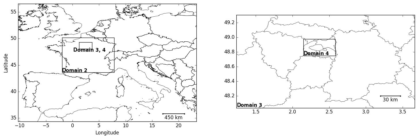
Figure 1Regional-scale domains: Europe (domain 1, with a spatial resolution of 45 km ×45 km), France (domain 2, with a spatial resolution 9 km ×9 km) and the Île-de-France region (domain 3, with a spatial resolution 3 km ×3 km) for one-way nesting simulations using Polair3D, as well as Paris (domain 4, with a spatial resolution of 1 km ×1 km) for simulations with SinG.
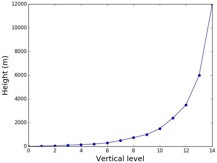
Figure 2Vertical levels used in all regional-scale simulations performed with Polair3D and SinG.
The initial and boundary conditions of the largest domain (over Europe) are obtained from a global-scale chemical-transport simulation using MOZART-4 (Model for Ozone and Related Chemical Tracers) (Emmons et al., 2010) coupled to the aerosol module GEOS-5 (Goddard Earth Observing System Model) (Chin et al., 2002). The spatial resolution of the MOZART-4/GEOS-5 simulation is , with 56 vertical levels.
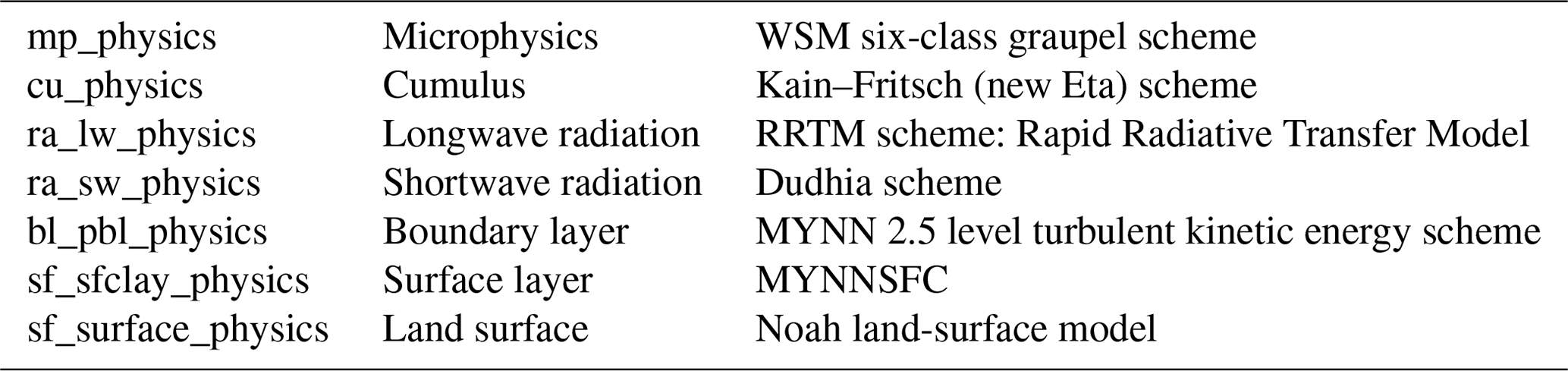
Meteorological data for the four domains are calculated by the Weather Research and Forecasting (WRF) model version 3.9.1.1 with a two-way nesting (Skamarock et al., 2008), employing the same spatial resolutions as used in Polair3D nesting simulations (45 km ×45 km, 9 km ×9 km, 3 km ×3 km and 1 km ×1 km for domains 4 to 1, respectively), with 38 vertical levels from 0 to 21 km. Observational data for wind speed, wind direction, pressure and temperature from the Paris Orly meteorological station are used as input data for the simulations over Paris (domain 4) using the nudging point technique. WRF domains are represented in Fig. 3, and Table 1 indicates the main physical options employed in WRF simulations.
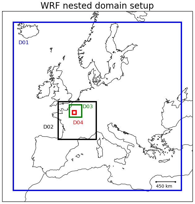
Figure 3Simulated domains using WRF to calculate meteorological data: Europe (D01, with a spatial resolution of 45 km ×45 km), France (D02, with a spatial resolution of 9 km × 9 km), the Île-de-France region (D03, with a spatial resolution of 3 km ×3 km) and Paris (D04, with a spatial resolution of 1 km ×1 km).
Dry deposition velocities of gas species are estimated following Zhang et al. (2003) and below-cloud scavenging following Sportisse and Du Bois (2002); see Sartelet et al. (2007) for more details on the deposition schemes used. Biogenic emissions over all domains are estimated using the Model of Emissions of Gases and Aerosols from Nature (MEGAN v2.04). Concerning anthropogenic emissions, over domains 1, 2 and outside Île-de-France over domain 3, they are calculated using the EMEP (European Monitoring and Evaluation Program) emission inventory for the year 2014, with a spatial resolution of .
Over Île-de-France in domain 3 and over domain 4, they are calculated using the emission inventory of 2012 provided by the air-quality agency of Paris (AIRPARIF). Comparisons between the 2012 AIRPARIF inventory and the more recent 2015 AIRPARIF inventory show that the largest differences in NOx emissions between the two years are due to differences in traffic emissions. For traffic emissions, fleet and technology data specific to 2013 and 2014 are used, and emissions are computed with the HEAVEN bottom-up traffic emissions model by AIRPARIF (https://trimis.ec.europa.eu/project/healthier-environment-through-abatement-vehicle-emission-and-noise, last access: 29 June 2020). Anthropogenic emissions followed the vertical distribution defined by Bieser et al. (2011) for the different activity sectors. More details on emission data and speciation may be found in Sartelet et al. (2018).
Note that in SinG, traffic emissions are only considered at the local scale and not at the regional scale to avoid double counting of emissions, as shown in Fig. 4.
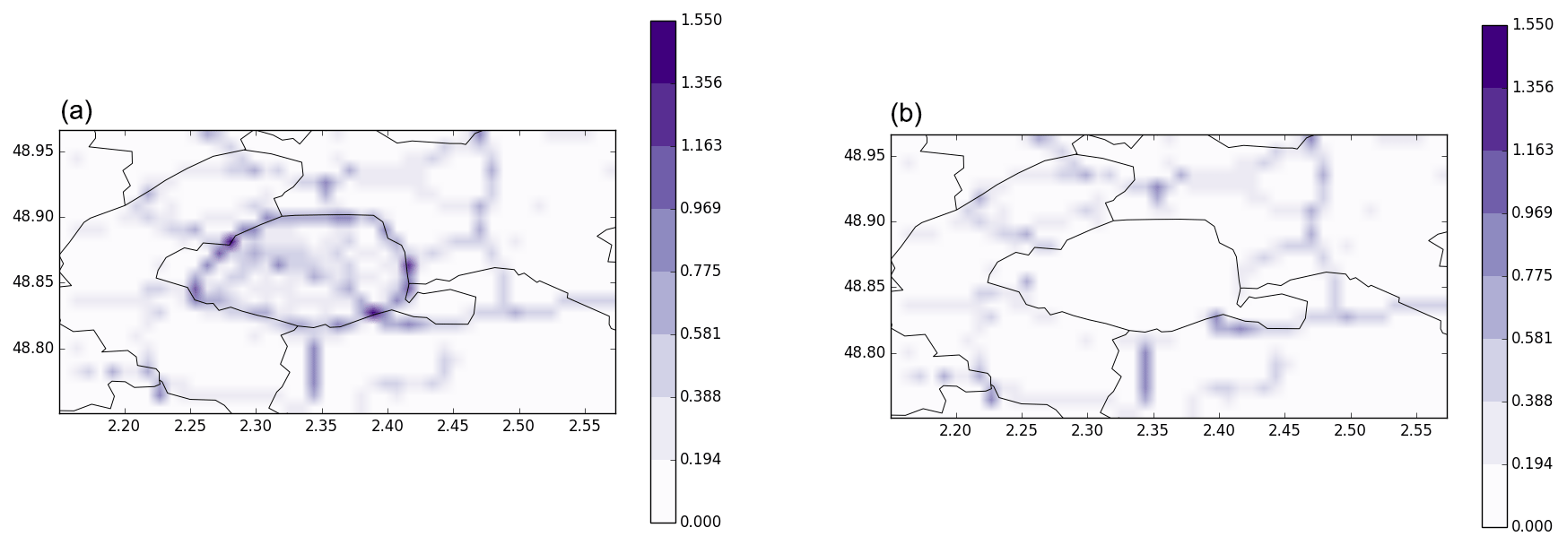
Figure 4Average over the simulated period of NO2 anthropogenic emissions (µg s−1 m−2) used as input for the regional-scale simulations over Paris with Polair3D (a) and as input for the regional-scale module of the multi-scale simulations with SinG (b).
3.2 Setup of local-scale simulations
The street network used in this study was provided by AIRPARIF. It contains the main streets of Paris, totalling 3819 streets. Apart from the location and length of the street segments, the street average dimensions (height and width) need to be defined.
A processing tool was developed to treat three different databases to determine street dimensions. The street widths are computed by summing the pavement width (from the BDTOPO database, available at http://professionnels.ign.fr/bdtopo, last access: 29 June 2020) and the two sidewalk widths (from an open-source public database “opendataparis“, available at https://www.data.gouv.fr/fr/datasets/trottoirs-des-rues-de-paris-prs/, last access: 6 June 2019). The street heights are determined using the Parisian urban planning agency (APUR) database (https://www.apur.org/fr, last access: 29 June 2020). The average height adopted at each street is calculated considering the mean height of all buildings located near the street axis, with a maximal distance of 10 m.
For the validity of the MUNICH model, building heights cannot be higher than the first vertical level of the regional model, so a maximum height of 30 m is adopted in this study. This limitation is acceptable over Paris because the average height of buildings is about 15 m. A minimum street width equal to 10 m is adopted over the whole domain, imposing a 10 m width for very narrow streets.
A few street segments in the domain, especially along the ring road around Paris (“boulevard périphérique”), are tunnels. For those segments, traffic emissions are not assigned to the segment itself but to two “virtual” streets added at each tunnel extremity, with half of the tunnel emissions each. The width of these virtual streets is the same as the width of the tunnel, and an arbitrary length of 3 m is chosen.
As Paris has a significant number of public parks and gardens, the average vegetation height is also considered for streets along these areas, and the model considers the street height to be the average height of buildings and trees. The average tree height is estimated to be about 13 m, considering the whole domain. It is calculated using a database containing the height of all trees in public spaces of Paris (“opendataparis”, available online at https://opendata.paris.fr/explore/dataset/les-arbres/information/, last access: 29 June 2020).
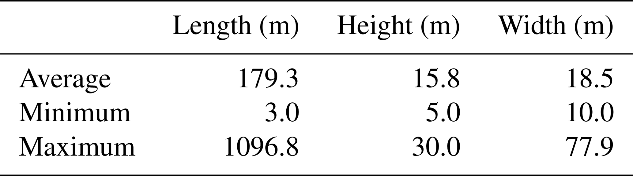
The street network and street characteristics are used for local-scale simulations using MUNICH and SinG, whereby wind profile and turbulent exchange depend on the aspect ratio αr (as mentioned in Sect. 2.2) of the streets. Table 2 indicates the maximum, average and minimum street dimensions of the whole street network used in this study.
Table 2Maximum, average and minimum street dimensions of the whole street network used in this study.
Emission data over the street segments are provided by AIRPARIF using the HEAVEN model (see Sartelet et al., 2018). Figure 5 illustrates the average emissions of NO2 during the simulation period. The highest emissions are located along the ring road (“boulevard périphérique”), as expected. This zone represents the most important road traffic in Paris.
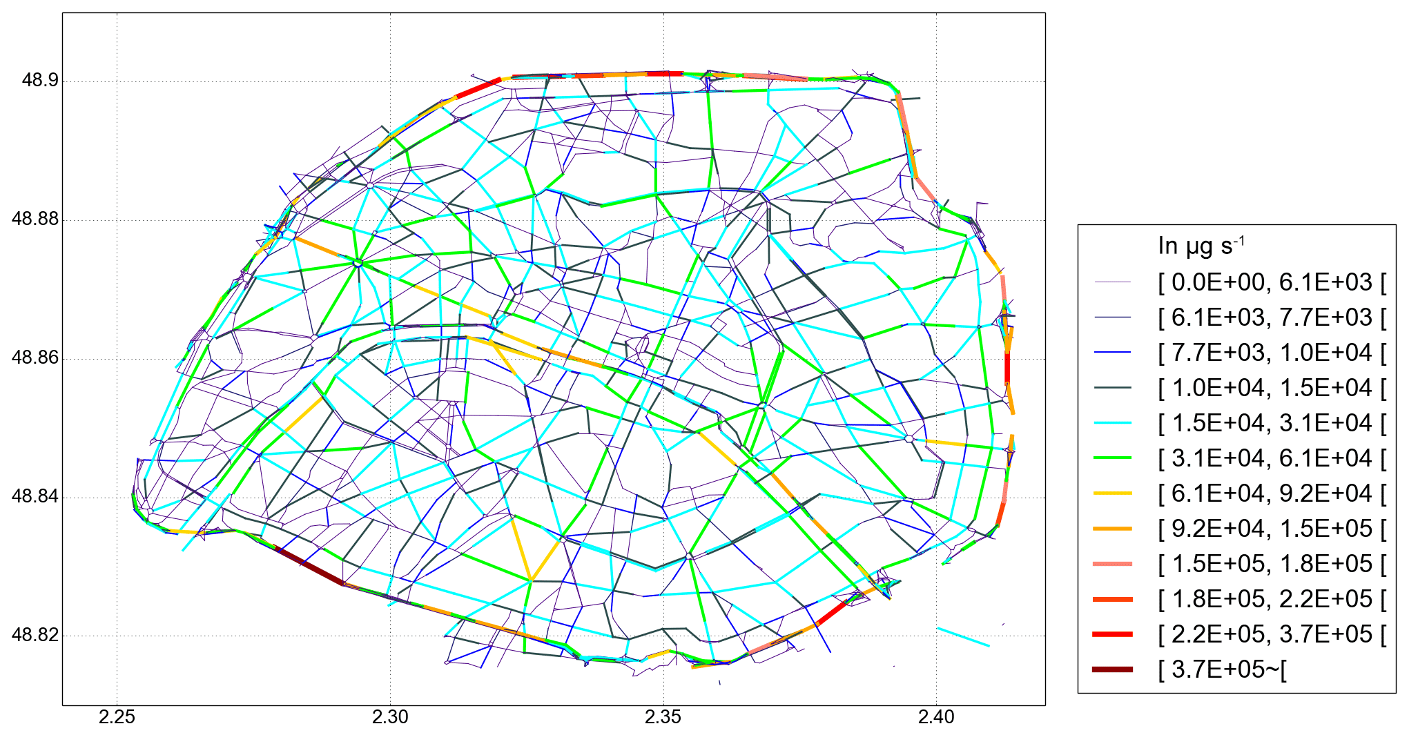
Figure 5Average traffic emissions of NO2 (µg s−1) calculated for local-scale simulations.
Meteorological data for each street and intersection are obtained from the WRF simulations, as in the regional-scale simulation over Paris. MUNICH simulations also require background concentrations as input data. They are obtained from Polair3D simulations over the Paris regional-scale domain. Note that the Polair3D simulations use all emissions, including traffic, as input data (as indicated in Fig. 4) and that Polair3D, SinG and MUNICH simulations are performed using the same temporal resolution.
3.3 List of simulations
Different numerical simulations are performed in order to compare the concentrations computed by SinG and MUNICH, as listed below. Numerical parameters (main time step) and the model hypothesis (stationary hypothesis or not) are analyzed. The main time step corresponds to the splitting time step between transport and chemistry in the regional-scale chemistry-transport model Polair3D. As in Polair3D, in MUNICH and SinG, the main time step corresponds to the time step used to split local-scale transport and chemistry if the stationary hypothesis is used. If the stationary hypothesis is not made, then the splitting time step between local-scale transport and chemistry is estimated and adjusted as detailed in Sect. 2.2. In SinG, the main time step also corresponds to the splitting time step between the regional-scale (Polair3D) and local-scale (MUNICH) modules. Different simulations are conducted with a main time step equal to 100 or 600 s and with or without the stationary hypothesis in MUNICH and SinG, as detailed in Table 3.
Table 3List of the sensitivity simulations performed using both MUNICH and SinG with different time steps (100 and 600 s) and adopting (or not) the stationary hypothesis.

Simulated concentrations are compared with air-quality measurements at traffic and urban background stations. Figure 6 represents the street-network emissions used in this study (see Sect. 3.2), also displaying the regional-scale grid mesh and the position of all stations considered. Air-quality stations comprise five urban stations (indicated by PA04C, PA07, PA12, PA13 PA18; blue dots) and eight traffic stations (BONAP, ELYS, HAUSS, CELES, BASCH, OPERA, SOULT and BP_EST; red dots).
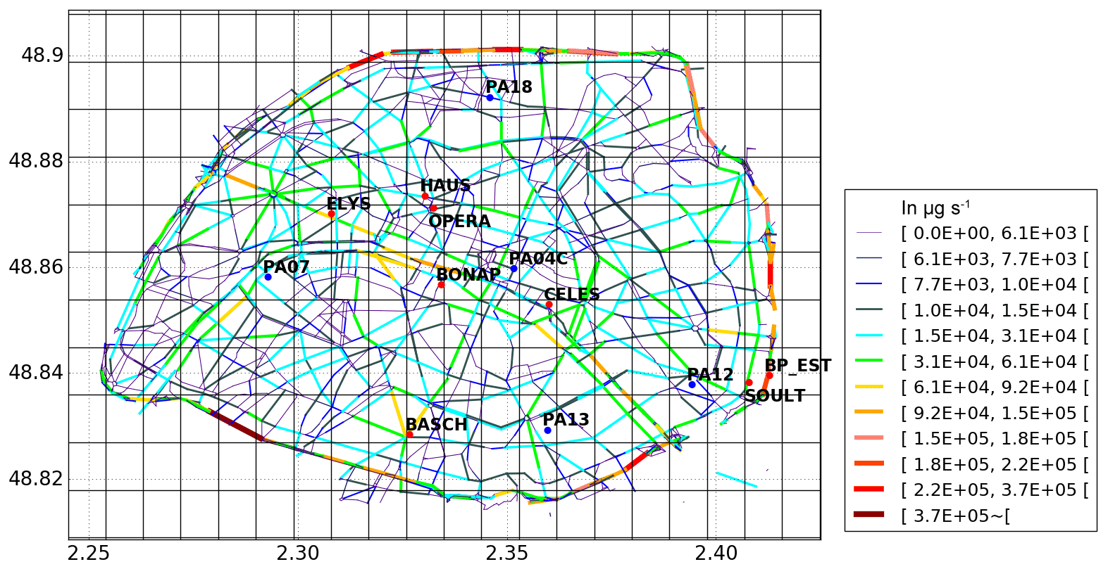
Figure 6Street network with the regional-scale grid mesh and the position of the measurement stations.
As mentioned in Sect. 3.3, different simulations with MUNICH and SinG are performed with different time steps, considering or not considering the stationary hypothesis. Figures 7 and 8 represent the time evolution of average daily concentrations of NOx, NO2 and NO during the simulation period, as simulated with MUNICH and SinG, at CELES station. NOx concentrations are independent of whether the stationary hypothesis is made or not and of the choice of the main time step. However, in both MUNICH and SinG, street concentrations of NO2 and NO are highly dependent on the choice of the time step when the stationary approach is used. This problem is solved with the nonstationary simulations, wherein street concentrations of NO2 and NO are numerically stable and independent of the choice of the main time step. For example, regarding the concentrations simulated at CELES station by MUNICH with the stationary approach, the modification of the time step from 600 to 100 s decreased NO2 concentrations by 5 % and increased NO concentrations by 12 %. With the nonstationary approach, these differences are reduced to 0.1 % for NO2 concentrations and 0.2 % for NO concentrations. Note that there are differences in the background concentrations of the regional-scale model if a time step of 600 s is used rather than 100 s. This explains the small differences in NO2 concentrations observed at CELES station in Fig. 8 using SinG with two different time steps (100 and 600 s) and the nonstationary approach. Therefore, in the rest of this paper only the simulations performed with the nonstationary approach and a main time step of 100 s are analyzed. Besides the numerical stability, NO2 and NO average concentrations simulated using the nonstationary approach are closer to observations than those simulated using the stationary approach, as shown in Figs. 7 and 8. The fraction bias of daily average concentrations calculated with SinG (with a 100 s time step) at CELES station is as high as 53 % and −24 % for NO2 and NO, respectively, using the stationary approach, and it is reduced to 13 % and 4 %, respectively, using the nonstationary approach.
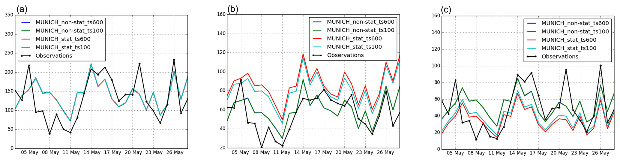
Figure 7Daily average concentrations of NOx (a), NO2 (b) and NO (c) concentrations (µg m−3) calculated by MUNICH at CELES station with different main time steps using the stationary and nonstationary approaches.
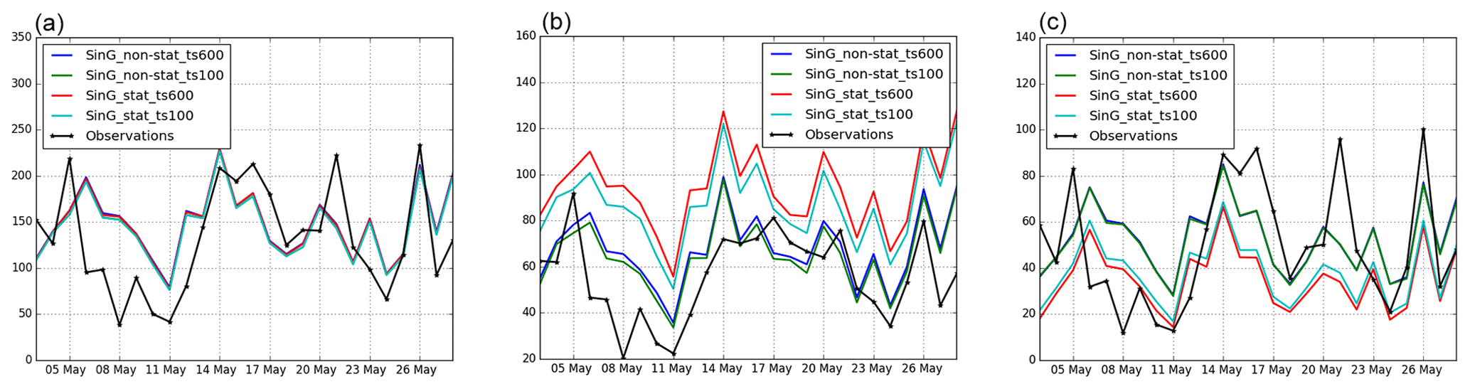
Figure 8Daily average concentrations of NOx (c), NO2 (b) and NO (c) concentrations (µg m−3) calculated by SinG at CELES station with different main time steps using the stationary and nonstationary approaches.
This section presents the comparisons between the measured concentrations of NO, NO2 and NOx and those simulated with MUNICH, Polair3D and SinG. As mentioned in Sect. 3.3, air-quality stations comprise eight traffic stations and five urban stations. The criteria applied to evaluate the comparisons are the statistics detailed in Hanna and Chang (2012) and Herring and Huq (2018): FB <0.3; 0.7< MG <1.3; NMSE <3; VG <1.6; FAC2 ≥0.5; NAD <0.3. Hanna and Chang (2012) and Herring and Huq (2018) also defined less strict criteria to be applied to urban areas: FB <0.67; NMSE <6; FAC2 ≥0.3; NAD <0.5. The definitions of these statistics are given in Appendix Sect. A1.
The statistics of the three models (Polair3D, MUNICH, SinG) for NO2 and NOx at traffic and background stations are indicated in Tables 4 and 5, respectively.
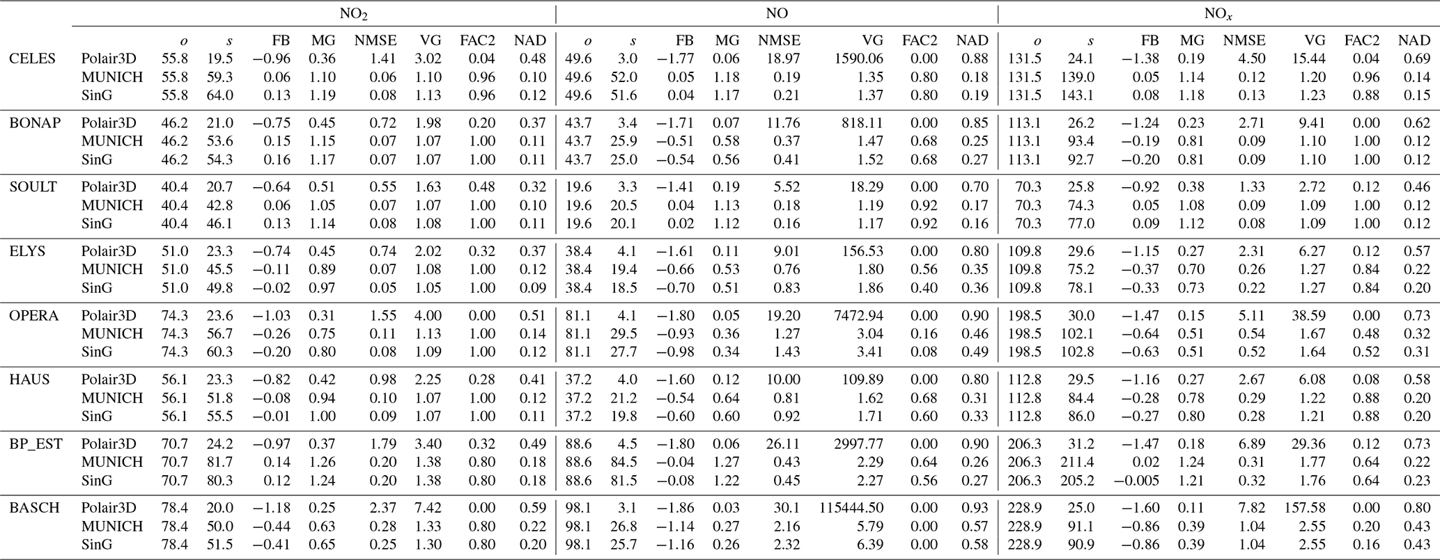
Table 4Statistical parameters* at traffic stations (o and s represent the average observed and simulated concentrations, respectively; µg m−3).
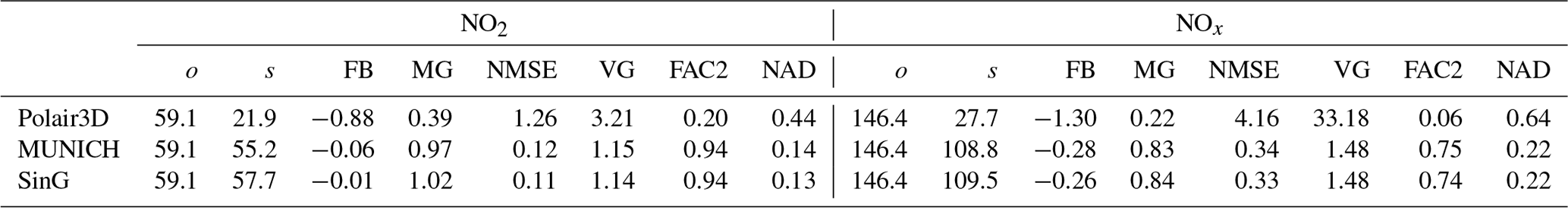
FB represents the fractional bias, MG the geometric mean bias, NMSE the normalized mean square error, VG the geometric variance, NAD the normalized absolute difference, and FAC2 the fraction of predictions within a factor of 2 of observations. They are calculated as detailed in Sect. A1.
Table 5Statistical parameters* at background stations (o and s represent the average observed and simulated concentrations, respectively; µg m−3).
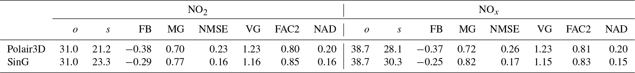
FB represents the fractional bias, MG the geometric mean bias, NMSE the normalized mean square error, VG the geometric variance, NAD the normalized absolute difference, and FAC2 the fraction of predictions within a factor of 2 of observations. They are calculated as detailed in Sect. A1.
5.1 Traffic stations
As expected, Polair3D strongly underestimates NO2 and NOx concentrations at traffic stations, as shown by the statistical indicators in Table 4, and the performance criteria defined by Hanna and Chang (2012) and Herring and Huq (2018) are not respected. However, NO2 and NOx concentrations are well modeled using both MUNICH and SinG.
As shown in Table 4, both MUNICH and SinG present similar statistics at the local scale, respecting the most strict performance criteria determined by Hanna and Chang (2012) for NO2 and NOx. Compared to MUNICH, the multi-scale approach of SinG improves the average statistical parameters for both pollutants.
The statistics at each station (see Sect. A2) show that the less strict criteria of Hanna and Chang (2012) indicated for urban areas are satisfied at all stations for NO2 concentrations using MUNICH and SinG. The most strict criteria are even respected at all stations except BASCH. In both MUNICH and SinG simulations, NO concentrations tend to be underestimated, although the performance criteria are verified at six out of eight stations. This underestimation may be due to the short lifetime of NO, leading to high uncertainties in dispersion and questioning the assumption of uniform concentrations in the street. The NO underestimation is the most significant at stations located in big squares (OPERA and BASCH), indicating that the airflow parameterization for big squares may need to be improved. Note that because of the underestimation of NO concentrations at OPERA and BASCH, the performance criteria for NOx are not respected at BASCH, and only the less strict performance criteria are respected at OPERA.
The daily evolution of NOx, NO2 and NO concentrations is well simulated, as shown in Figs. 9 and 10, which display the time evolution of daily concentrations of NOx, NO2 and NO simulated with MUNICH, SinG and Polair3D at CELES and SOULT stations. However, NO2 concentrations are overestimated at almost all stations from 9 to 11 May. This period corresponds to a French holiday, suggesting that the temporal variability of emissions needs to be modified in the model for those days. Beyond daily average concentrations, both SinG and MUNICH represent the time evolution of hourly concentrations well, as shown in Fig. 11. The better agreement of SinG and MUNICH during the morning peak than the evening one may be due to difficulties in modeling the atmospheric boundary height in the evening and to higher day-to-day variability of traffic emissions in the evening than in the morning.
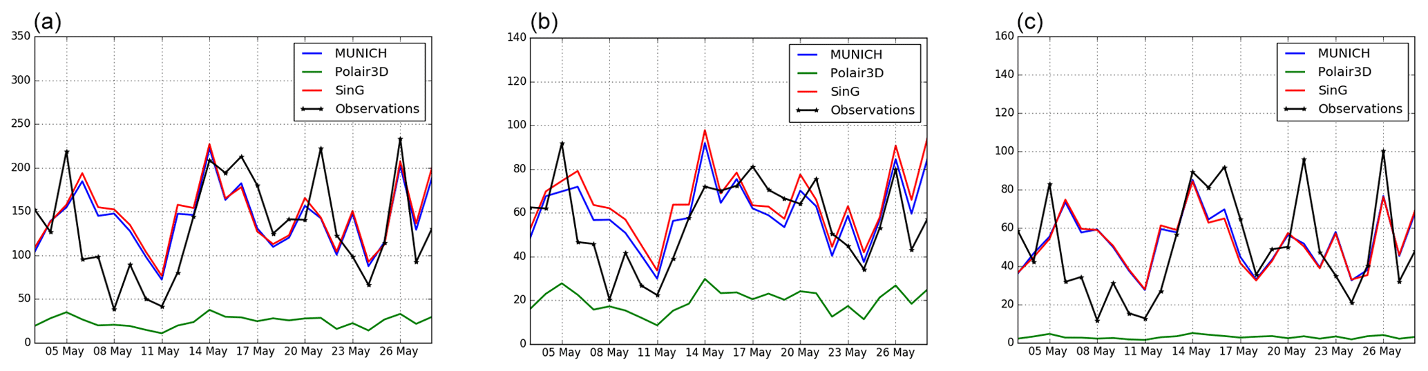
Figure 9Daily average NOx (a), NO2 (b) and NO (c) concentrations (µg m−3) observed and simulated at CELES station with MUNICH, SinG and Polair3D.
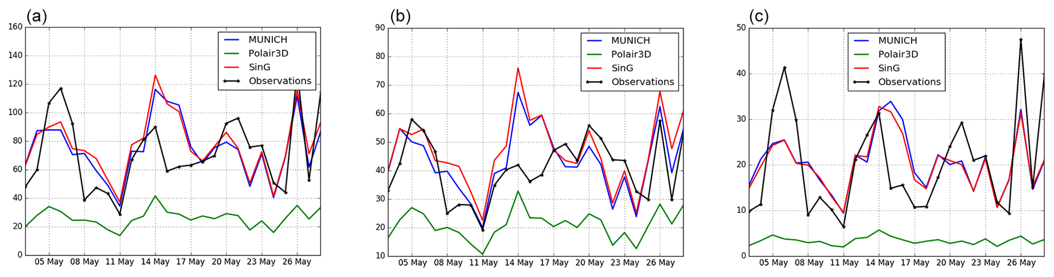
Figure 10Daily average NOx (a), NO2 (b) and NO (c) concentrations (µg m−3) observed and simulated at SOULT station with MUNICH, SinG and Polair3D.
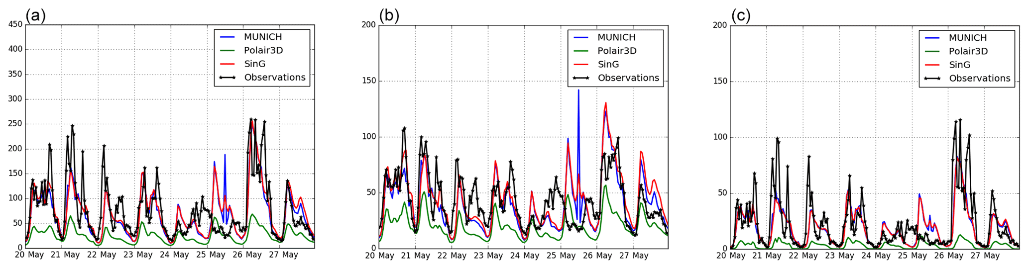
Figure 11Hourly average NOx (a), NO2 (b) and NO (c) concentrations (µg m−3) observed and simulated at SOULT station with MUNICH, SinG and Polair3D.
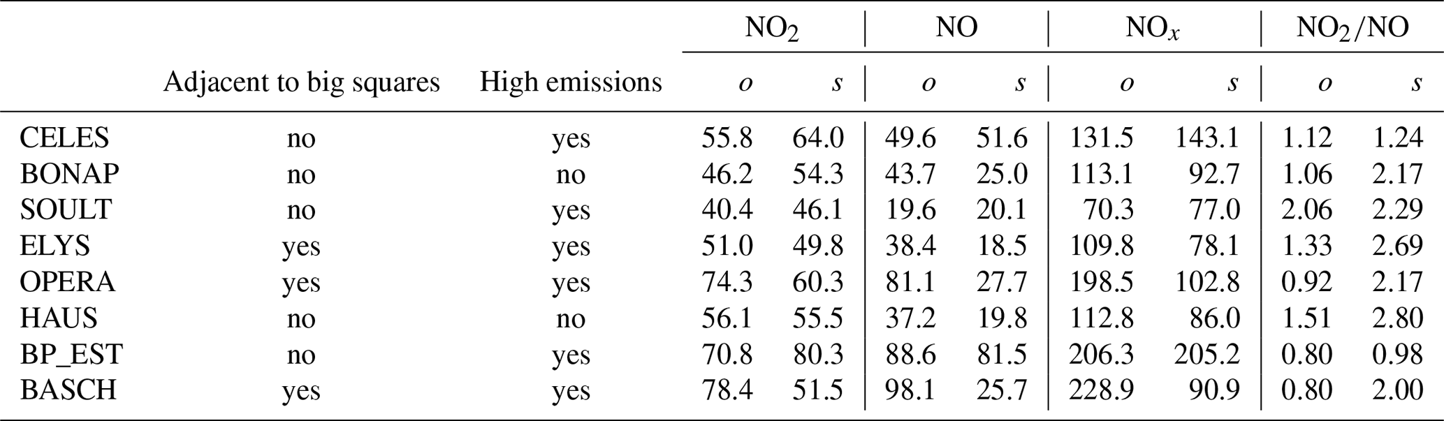
Table 6 indicates the average values of air-quality measurements and SinG concentrations, as well as the corresponding ratios of NO2∕NO. The ratios are overestimated in the simulations: they vary between 0.80 and 2.06 in the measurements and between 0.98 and 2.80 in the simulations. The ratios are well simulated at CELES, SOULT and BP_EST stations, which are located in streets with high traffic emissions. However, they are overestimated at other stations, such as those in big squares (OPERA, BASCH). This may be due to the short lifetime of NO, for which the assumption of uniform concentrations in wide streets and big squares may not be verified.
Table 6Average concentrations measured and simulated with SinG of NOx, NO2, NO and NO2∕NO ratios at traffic stations (o and s represent the observed and simulated average, respectively; µg m−3).
5.2 Background stations
Although both SinG and Polair3D perform well at simulating background NO2 and NOx concentrations, the multi-scale approach with SinG improves the statistics of comparisons to measurements at urban background stations. Table 5 presents the statistics at urban background stations for the NO2 and NOx concentrations simulated with Polair3D and SinG. The multi-scale approach used in SinG improved all statistical parameters, especially the fractional bias, for both NO2 and NOx. Regarding the simulated period, SinG respects the most strict performance criteria defined by Hanna and Chang (2012).
As expected, the differences between NOx concentrations simulated with SinG and Polair3D are the highest at stations where vehicular traffic is high. Figures 12 and 13 show the time evolution of daily NO, NO2 and NOx concentrations at the background stations PA04C and PA13. PA04C is a station located near an important traffic area, while PA13 is located in an area with lower vehicle flux. SinG and Polair3D differences are more important at PA04C station than at PA13 station. More details about the differences of Polair3D and SinG concentrations are described in Sect. 6.2.
Even though both SinG and Polair3D represent the measured background concentrations well, the two-way coupling between spatial scales in SinG improves the modeling of NO2, NO and NOx background concentrations. Furthermore, SinG proved to represent NO2 and NOx concentrations well at both local (traffic stations) and regional (background stations) scales.
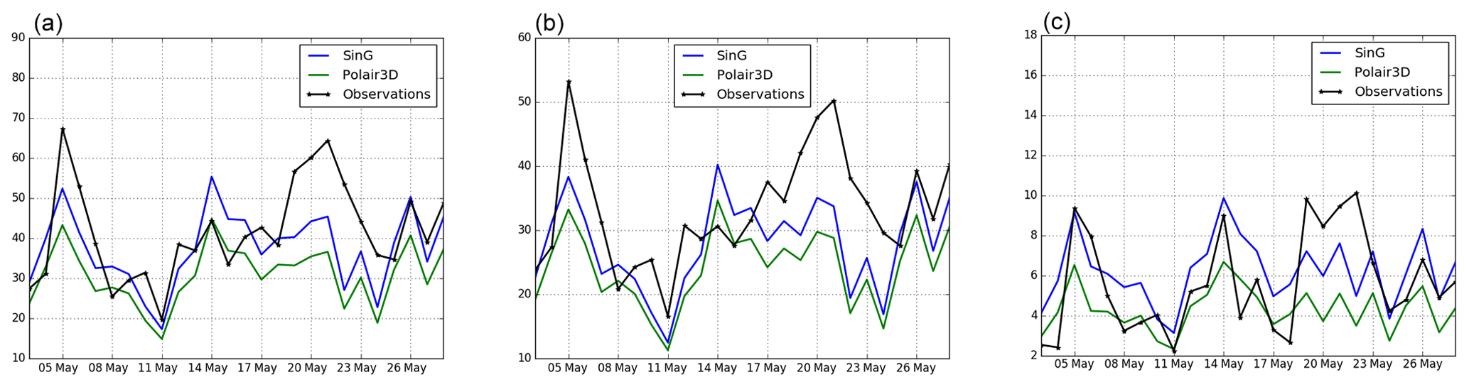
Figure 12Daily average concentrations of NOx (a), NO2 (b) and NO (c) (µg m−3) observed and simulated at PA04C station with SinG and Polair3D.
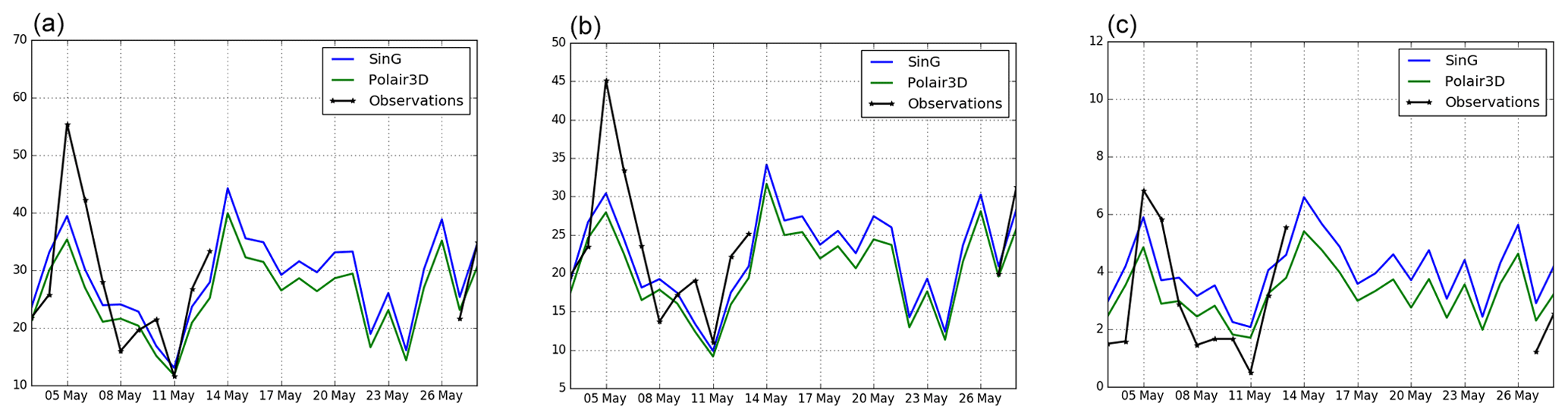
Figure 13Daily average concentrations of NOx (c), NO2 (b) and NO (c) (µg m−3) observed and simulated at PA13 station with SinG and Polair3D.
This section analyzes the influence of the two-way dynamic coupling between the regional and local scales on NO, NO2 and NOx concentrations. This influence is analyzed by comparing the concentrations simulated with SinG and MUNICH at the local scale (in streets) and SinG and Polair3D at the regional scale (background concentrations). The influence of different factors influencing this coupling is evaluated: the geometric characteristics of the streets, the inlet and output mass fluxes in the streets, and the intensity of traffic emissions.
At both the regional and local scales, larger differences between coupled and non-coupled simulations are observed in high traffic emission areas. In these areas the vertical mass transfer between the local and regional scales tends to be more important for two main reasons: (i) the gradient between the street and the background concentrations is larger when traffic emissions are higher (see Eq. 8), and (ii) higher traffic emissions lead to a higher influence of the mass advection flux between streets by mean wind and therefore a higher influence of vertical mass transfer at street intersections. If the vertical mass transfer is high, then the background concentrations may be higher in the two-way approach of SinG than in the one-way approach of MUNICH, leading to higher concentrations in streets. Figure 14 represents the mean relative differences between NO2 concentrations simulated using coupled and non-coupled simulations at local (differences between SinG and MUNICH) and regional scales (differences between SinG and Polair3D), averaged over the simulation period. On average, these mean relative differences are about 7.5% at the local scale and 11.3 % at the regional scale. To compute these relative differences, MUNICH and Polair3D concentrations were adopted as reference concentrations at the local and regional scales, respectively. The influence of dynamic coupling is now studied in more detail, first at the local scale (in streets) and then at the regional scale.
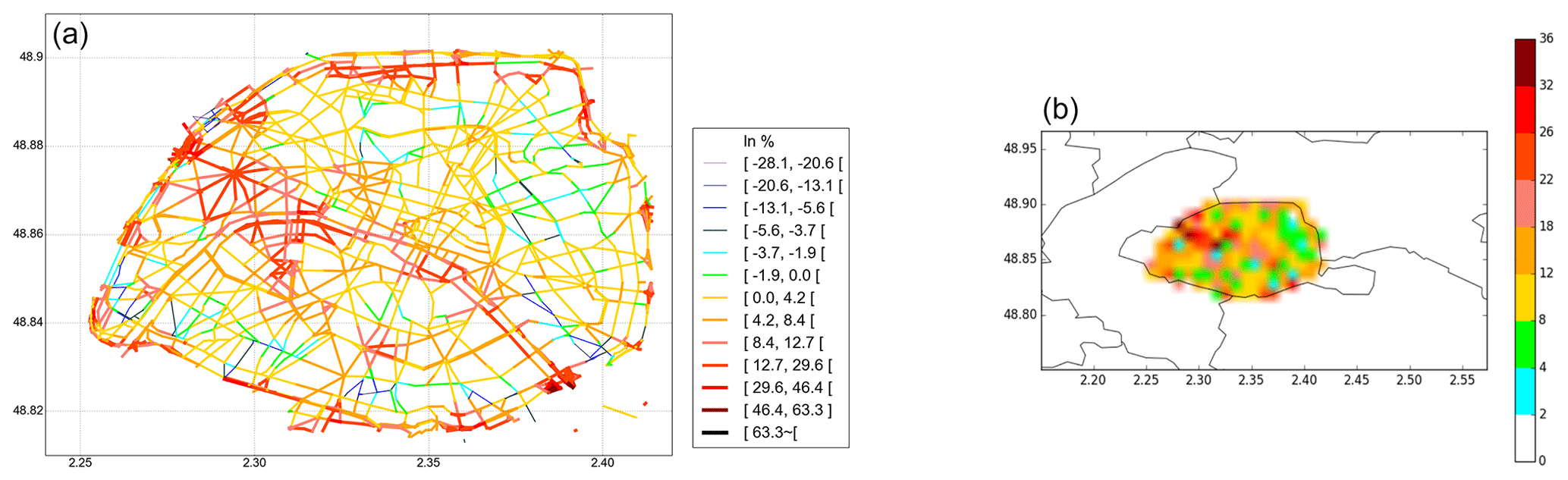
Figure 14Relative differences (%) between NO2 concentrations simulated by SinG and MUNICH at the local scale (a) and by SinG and Polair3D at the regional scale (b).
6.1 Local scale
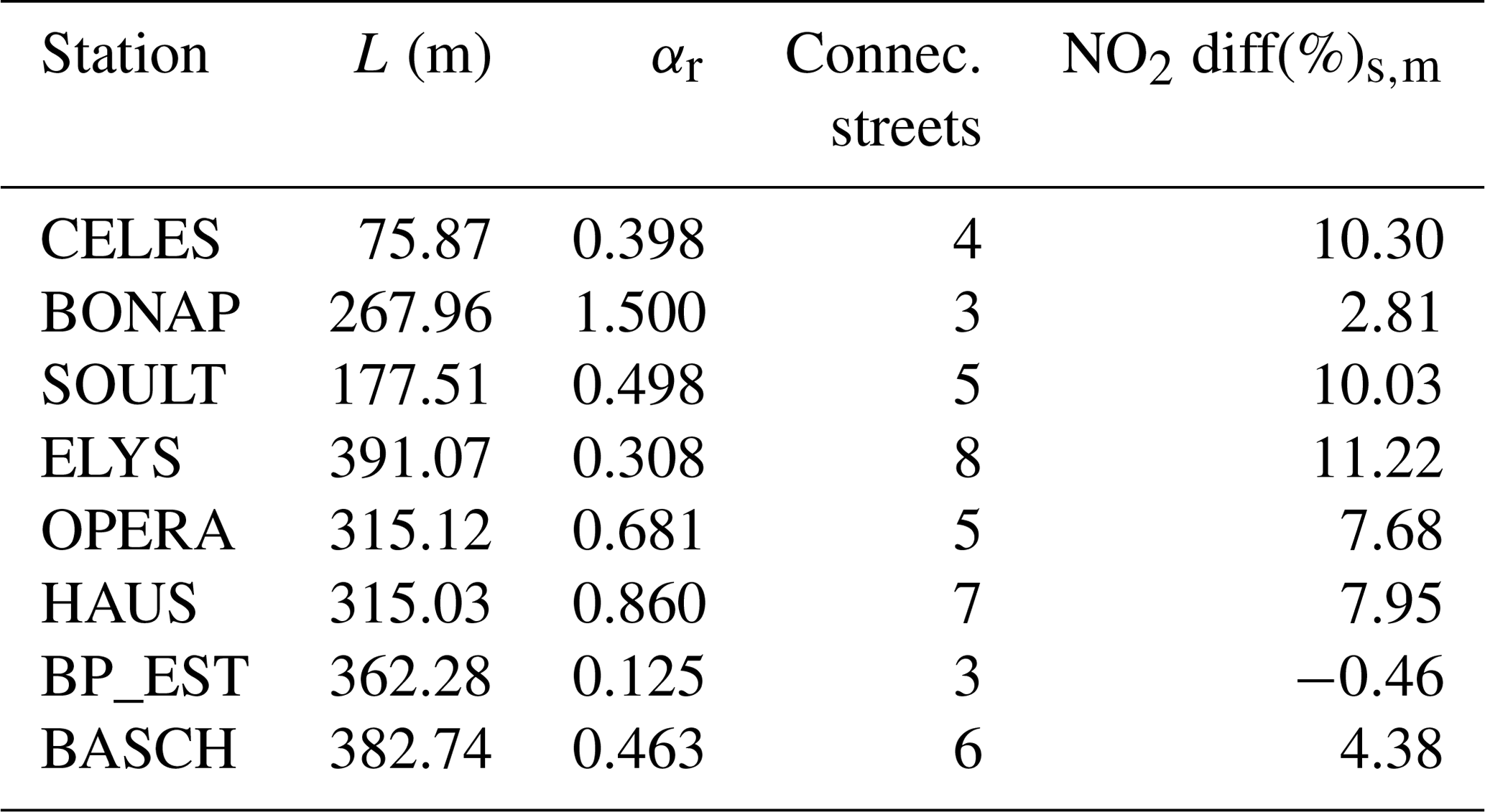
The differences between SinG and MUNICH are first analyzed at traffic stations. In SinG, the coupling depends on the concentration gradients between the street and the background but also on the street dimensions, the standard deviation of vertical wind speed, and input–output mass fluxes at intersections. Table 7 summarizes the street characteristics, with L the street length, αr the street aspect ratio, and NO2 diff(%)s,m the mean relative difference between NO2 concentrations simulated with SinG and MUNICH over the simulation period. The differences between SinG and MUNICH concentrations are quite low: they are lower than 12 % at each of the eight traffic stations. In agreement with Sect. 5.1 and Table 4, NO2 concentrations simulated with SinG tend to be larger than those simulated with MUNICH because the background concentrations in SinG are influenced by the high NOx concentrations of the street network.
Table 7Street length (L), aspect ratio (αr), number of connected streets, and the corresponding relative difference of NO2 concentrations calculated by SinG and MUNICH at each traffic station.
As explained in Sect. 2.3, SinG transfers the vertical mass flux from streets and intersections to the regional scale to correct background concentrations. Therefore, the differences between MUNICH and SinG simulations are mostly due to differences in background concentrations. The time variations of the differences are illustrated in Fig. 15, which represents the time evolution at CELES station of NO2 concentrations in the streets and the background using MUNICH and SinG. The differences between the street and the background concentrations are strongly correlated. The higher the differences between SinG and MUNICH background concentrations, the higher the differences between SinG and MUNICH street concentrations.
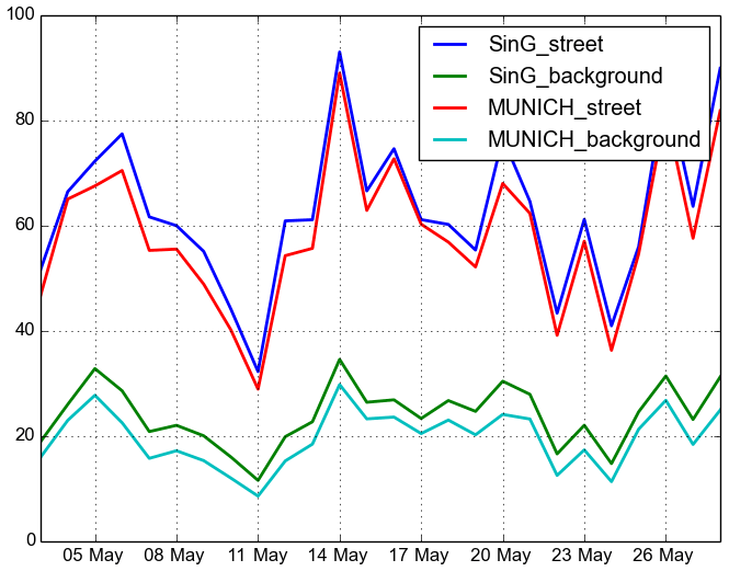
Figure 15NO2 daily average concentrations (µg m−3) in the street and in the background using MUNICH (one-way dynamic coupling) and SinG (two-way dynamic coupling) at CELES traffic station.
However, as indicated in Table 7, the magnitude of the differences between SinG and MUNICH depends very much on the street: the lowest differences between SinG and MUNICH NO2 concentrations are simulated at the stations BONAP and BP_EST, with differences below 3 %, while the highest differences are simulated at the stations CELES, SOULT and ELYS, with differences around 10 %.
To understand why the two-way coupling between the background and the streets differs depending on stations, the differences between SinG and MUNICH are analyzed in terms of the daily-weighted mass fluxes that influence the street concentrations. As detailed in Sect. 2.2, the street concentrations are influenced by the vertical mass flux from and to background concentrations (Qvert), but also the emission mass flux (Qemis) and the mass fluxes from the street lateral boundaries (Qinflow, Qoutflow). Daily-weighted mass fluxes () are calculated according to
with
Figure 16 shows the daily-weighted mass fluxes influencing the street concentrations at BONAP, CELES and BP_EST. At BONAP, advection (inlet and outlet fluxes in Fig. 16) dominates over vertical transfer, probably because the value of αr is high, indicating that the street is narrow. At BP_EST, Fig. 16 indicates that vertical transfer is the dominant process. This dominance of vertical transfer is because the street is large and the value of αr is low. Note that BP_EST station also presents a high emission flux, with data common to both models SinG and MUNICH. Also, both BP_EST and BONAP present a low number of connected streets, which may indicate an inferior vertical mass flux intersection compared to other traffic stations. At CELES, where the value of αr is intermediate, the inlet, outlet and vertical fluxes have the same order of magnitude, and the differences between MUNICH and SinG are larger than at BONAP and BP_EST stations.
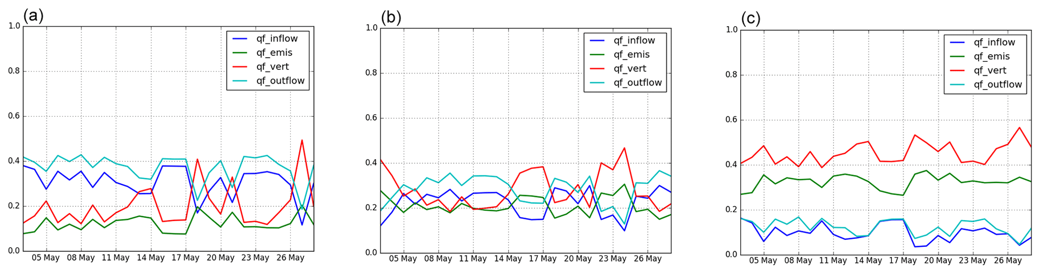
Figure 16Normalized daily-weighted mass fluxes of NO2 at BONAP (a), CELES (b) and BP_EST (c) traffic stations: inflow advection mass flux (qf_inflow) in blue, emissions (qf_emis) in green, vertical mass flux (qf_vert) in red, and outflow advection mass flux (qf_outflow) in cyan. The fluxes are calculated as detailed in Eq. (18).
NO concentrations are less sensitive to the two-way coupling between local and regional scales than NO2 concentrations, and the average concentrations simulated with SinG and MUNICH are very similar at all stations (as indicated in Sect. A2). This is explained by three factors: (i) NO background concentrations are very low compared to NO concentrations in streets; (ii) NO has a short lifetime, as it quickly reacts to form NO2; and (iii) NO concentrations in streets are mainly determined by direct emissions, which are the same in MUNICH and SinG simulations. Figure 17 shows the daily-weighted mass fluxes influencing the street concentrations at BONAP, CELES and BP_EST. At all three stations, the emission mass flux clearly dominates over the inlet–outlet and vertical mass fluxes, confirming the strong and local influence of NO emissions on NO concentrations.

Figure 17Daily-weighted mass flux of NO at BONAP (a), CELES (b) and BP_EST (c) traffic stations.
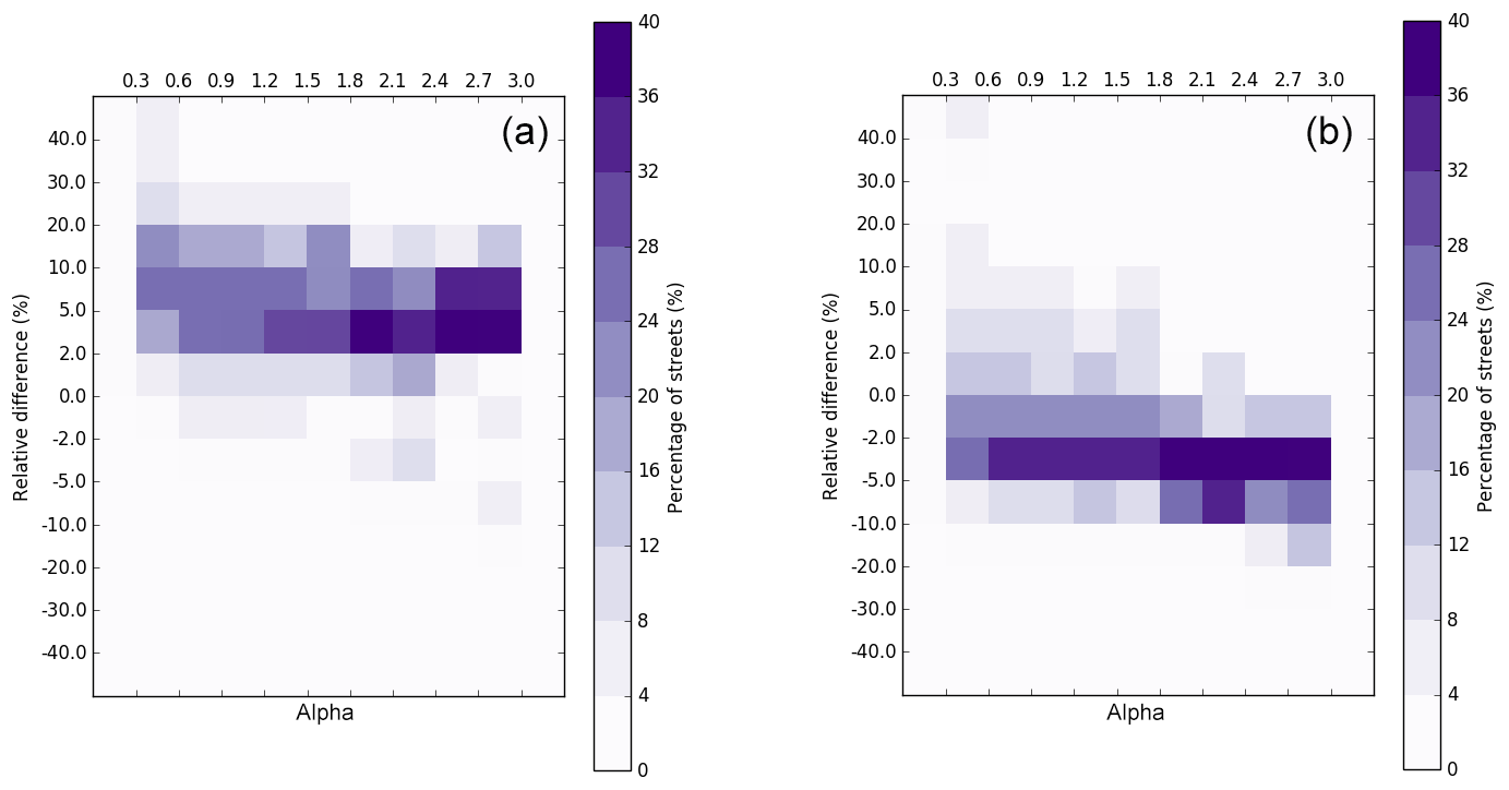
Figure 18Percentage of streets (purple) present in each αr interval according to αr values and the NO2 (a) and NO (b) relative differences between pollutant concentrations calculated by SinG and MUNICH.
To summarize, for NO concentrations, the two-way dynamic coupling between the regional and local scales tends not to be important. However, for NO2 concentrations, it seems to be more important at stations with low to intermediate values of αr for which the inlet, outlet and vertical fluxes have the same order of magnitude. In contrast, the two-way coupling seems to be less important at stations with low or high values of αr, where either the vertical flux or the inlet–outlet flux dominates over the other.
To better quantify the importance of the two-way coupling for the street concentrations, the concentrations simulated with SinG and MUNICH in each street are compared over the whole Paris street network. The relative differences between concentrations simulated with the two models are computed in each street. The average over all streets of these relative differences, as well as the minimum and maximum values, are estimated and discussed below.
NO, NO2 and NOx average concentrations simulated with SinG, as well as the mean relative differences between SinG and MUNICH, are represented in Sect. B, Fig. B1.
As was observed at traffic stations, the average NO2 concentrations are larger with SinG than MUNICH for most streets in the network, with an average relative difference over all streets of about 7.5 %. Although this relative difference is low, the maximum and minimum differences are high and reach 63 % and −28 %, respectively. The average NO concentration is slightly lower with SinG than MUNICH, and the average relative difference over all streets is low at about −0.85 %. As for NO2, for NO concentrations, there is a large variation between the maximum and minimum differences (58 % and −35 %, respectively). In particular, NO concentrations simulated with SinG are generally lower than those simulated with MUNICH in the center of the street network. However, in other places, such as the ring road, NO concentrations simulated with SinG are about 5 % higher than those simulated with MUNICH. Similarly to NO2, NOx concentrations also presented low average differences between SinG and MUNICH, about 5 % in the whole street network, but with high maximum and minimum values (60 % and −27 %, respectively). As discussed at the beginning of this section, relative differences between NO2, NO and NOx concentrations simulated with SinG and MUNICH are strongly correlated with the emissions in the street and with the street aspect ratio αr. Therefore, large differences between SinG and MUNICH are observed in streets with high traffic emissions and intermediate to low values of αr, such as in the ring road, where the vertical mass transfer between streets and the background is important. The differences are less pronounced for NO concentrations because of the short lifetime of NO.
As the majority of Parisian streets present an intermediate value of the street aspect ratio αr, to better understand the influence of the street aspect ratio on the dynamic coupling, the variations of the relative differences between NO2 and NO concentrations simulated with SinG and MUNICH with the street aspect ratio αr are studied. For the different ranges of αr encountered in the street network and for different ranges of relative differences, Fig. 18 presents the percentage of streets involved in the network. Thus, in the figure, the sum of each column is 100 %. In accordance with Fig. 14, NO2 average concentrations are in general higher using SinG than using MUNICH. The relative difference is mostly between 2 % and 30 % for streets with αr smaller than 1.8 and between 2 % and 10 % for streets with αr larger than 1.8. The higher the value of αr, the lower the variability of relative differences. However, even for αr larger than 1.8, relative differences between 10 % and 20 % are relatively frequent (between 16 % and 20 % of the streets), indicating the influence of factors other than the street aspect ratios.
For NO, the average concentrations simulated with SinG are in general smaller than those simulated with MUNICH, mostly between 0 % and −10 %. As for NO2, the variability of relative differences is higher for low to intermediate values of αr.
6.2 Regional scale
Figure B2 presents the spatial distribution of average background NO2 and NOx concentrations simulated with SinG and the relative differences to those simulated with Polair3D. As indicated in Sect. 5.2, background concentrations at the regional scale are influenced by the two-way coupling with the local scale. NO2 concentration differences between SinG and Polair3D are on average 11 %, with a maximum value of 34 %. For NOx concentrations, the relative differences are of the same order of magnitude as for NO2, with an average and a maximum value equal to 15 % and 42 %, respectively. NO concentrations are not shown in Fig. B2 because they are very low at the regional scale.
For both NO2 and NOx, the most important differences between Polair3D and SinG background concentrations are observed at the ring road and in the north-west of Paris. Similarly to the local scale, relative differences in the concentrations simulated with SinG and MUNICH are higher in regions with high traffic emissions and where streets present an intermediate value of αr, such as ELYS (see Fig. 6). Note that, as mentioned in Sect. 2.3, SinG output concentrations at the regional scale are an average of background and street concentrations in each grid cell. This justifies the higher differences between coupled and non-coupled simulations at the regional scale than at the local scale. Regarding the downwind side of Paris, the concentrations of NOx and O3 simulated by Polair3D and SinG are similar outside the street-network region.
In this study, a Street-in-Grid (SinG) multi-scale simulation is performed over Paris with a two-way dynamic coupling between the local (street) and regional (background) scales. For Paris, 3819 streets are considered, and different databases are used to determine the width and height of each street. A stationary approach may be used to compute pollutant concentrations in the streets by performing a mass balance between emission, deposition, and vertical and horizontal mass transfer. Although this approach is reasonable to estimate NOx concentrations or the concentration of inert pollutants, it is not appropriate to compute the concentrations of reactive pollutants such as NO2 or NO. A nonstationary dynamic approach was implemented by solving the transport of pollutants and chemistry with a second-order numerical scheme. This approach proved to be numerically stable, with good agreement between observed and simulated concentrations of NO2 and NOx at both regional and local scales.
In the streets, NOx and NO2 concentrations simulated by SinG compare well to measurements performed at traffic stations. For NO2 concentrations, the statistical indicators obtained with SinG and the street model (MUNICH) respect the most strict performance criteria (Hanna and Chang, 2012) at traffic stations. However, NO concentrations are strongly underestimated at traffic stations located in streets that converge in big squares. This underestimation is probably due to the short lifetime of NO, for which the assumption of uniform concentrations in wide streets and big squares may not be appropriate. At the regional scale, SinG also performs well in simulating NOx and NO2 concentrations, and the most strict criteria are respected at background stations.
The influence of the two-way dynamic coupling between the regional and local scales is assessed by comparing the concentrations simulated with SinG to those simulated with MUNICH. NOx and NO2 concentrations simulated with SinG and MUNICH are strongly correlated with traffic emissions, and the highest concentrations are observed in the ring road around Paris (“boulevard périphérique”) where emissions are the highest. Similarly, at both local and regional scales, the influence of the dynamic coupling is larger in areas where traffic emissions are high. NO2 concentrations simulated with SinG are in general larger than those simulated with MUNICH, especially in high emission areas, because the background concentrations in SinG are influenced by the high NOx concentrations of the street network. The influence of the two-way coupling depends not only on the emission strength, but also on the aspect ratio (height over width) of the street. Although, on average over the streets of Paris, the influence of the two-way coupling on NO2 concentrations in the street is only 7.5 %, it can reach values as high as 63 %. The influence of the two-way coupling on background regional NO2 concentrations can be large as well: 11 % on average over Paris with a maximum relative difference of 34 %. Because NO background concentrations are very low and because of the short NO lifetime, NO concentrations are less sensitive to two-way dynamic coupling than NO2.
A1 Definitions
-
FB: fractional bias
-
MG: Geometric mean bias
-
NMSE: normalized mean square error
-
VG: geometric variance
-
NAD: normalized absolute difference
-
FAC2: fraction of data that satisfy
In the above expressions, o and c represent the observed and simulated concentrations, respectively.
A2 Statistical parameters at all traffic stations
Table A1Statistical indicators at traffic stations for concentrations of NO2, NO and NOx.
B1 Local scale
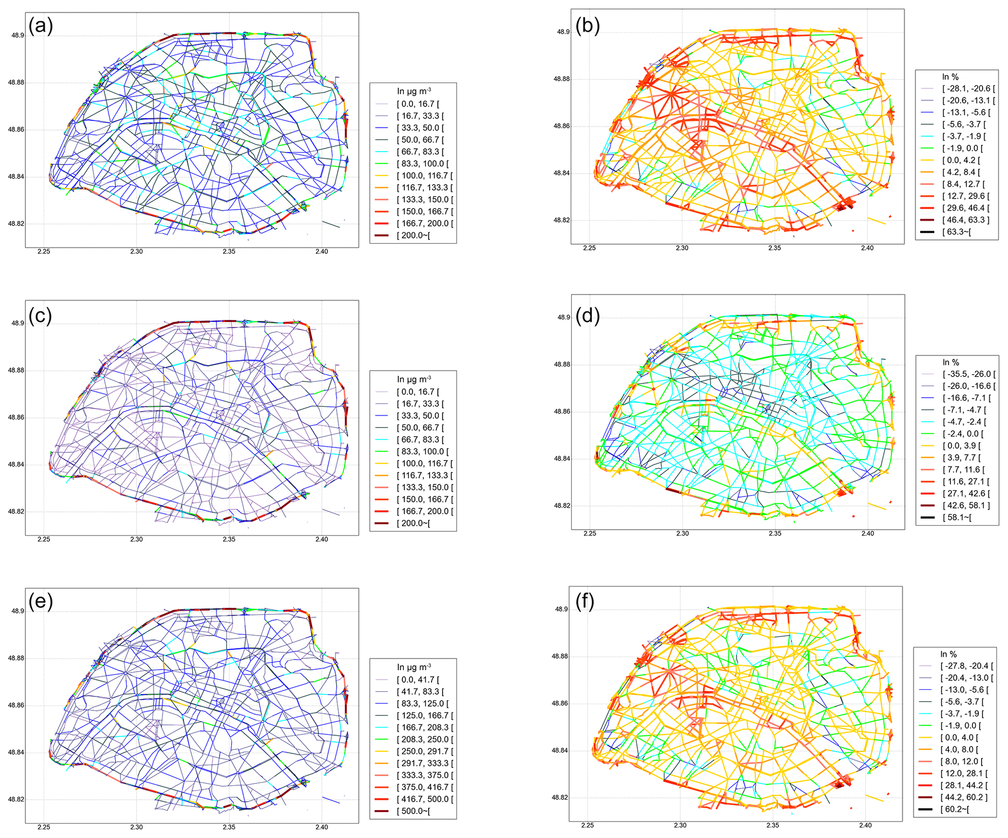
Figure B1NO2 (a, b), NO (c, d) and NOx (e, f) concentrations simulated over Paris with SinG (a) and relative differences between SinG and MUNICH (b).
B2 Regional scale
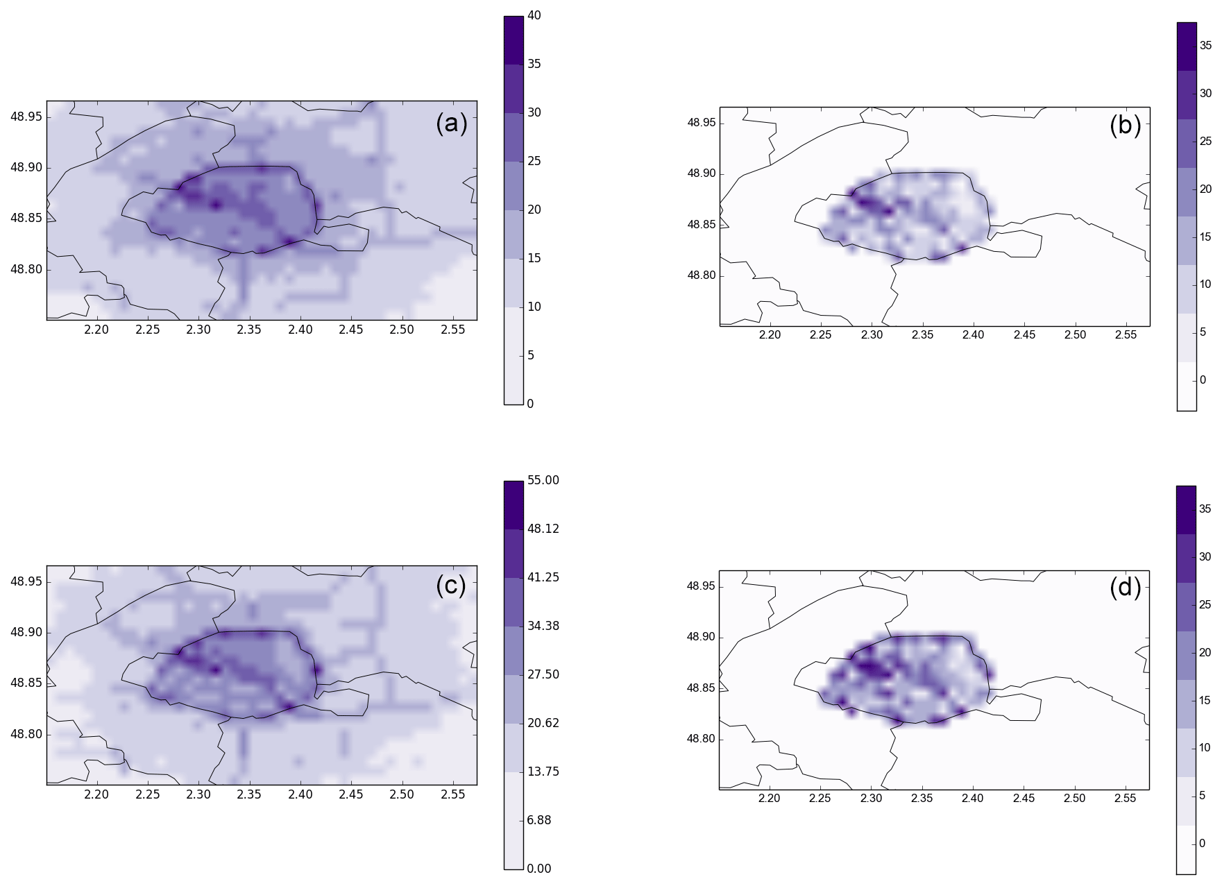
Figure B2NO2 (a, b) and NOx (c, d) concentrations simulated over Paris with SinG (a, c) and relative differences between SinG and Polair3D in percent (b, d).
The observation data are publicly available from AIRPARIF, Air quality – station data download, at http://airparif.fr/en/telechargement/telechargement-station (AIRPARIF, 2020). The model data are available upon request.
KS and LL were responsible for conceptualization. LL, KS and YK developed the software. LL conduced the visualization and validation; LL and KS performed the formal analysis. YK, JV and KS acquired resources. KS and OC were responsible for funding acquisition. LL and KS were responsible for writing and original draft preparation.
The authors declare that they have no conflict of interest.
This article is part of the special issue “Air Quality Research at Street-Level (ACP/GMD inter-journal SI)”. It is not associated with a conference.
The authors also thank AIRPARIF and the ANSES (the French agency for food safety, environment and labor) working group on ambient particulate matter for the traffic emission information. Yelva Roustan, Fabrice Dugay and Olivier Sanchez are gratefully acknowledged for discussions.
This research has been supported by the Department of Green Spaces and Environment (Mairie de Paris) and the École des Ponts ParisTech (grant CIFRE no. 2017/064).
This paper was edited by Barbara Ervens and reviewed by two anonymous referees.
Abdallah, C., Afif, C., El Masri, N., Öztürk, F., Keleş, M., and Sartelet, K.: A first annual assessment of air quality modeling over Lebanon using WRF/Polyphemus, Atmos. Pollut. Res., 9, 643–654, 2018. a
AIRPARIF: Air quality – station data download, available at: http://airparif.fr/en/telechargement/telechargement-station, last access: 30 June 2020. a
Ascher, U. and Petzold, L.: Computer Methods for Ordinary Differential Equations and Differential-Algebraic Equations, ISBN 978-0-89871-412-8, Philadelphia: Society for Industrial and Applied Mathematics, 1998. a
Berkowicz, R.: OSPM – A parameterised street pollution model, Environ. Monit. Assess., 65, 323–331, 2000. a
Berkowicz, R., Hertel, O., Larsen, S. E., Sørensen, N. N., and Nielsen, M.: Modelling traffic pollution in streets, Danish national environmental research institute, 1997. a, b
Bieser, J., Aulinger, A., Matthias, V., Quante, M., and van Der Gon, H. D.: Vertical emission profiles for Europe based on plume rise calculations, Environ. Pollut., 159, 2935–2946, 2011. a
Boutahar, J., Lacour, S., Mallet, V., Quélo, D., Roustan, Y., and Sportisse, B.: Development and validation of a fully modular platform for numerical modelling of air pollution: POLAIR, Int. J. Environ. Pollut., 22, 17–28, 2004. a
Brandt, J., Christensen, J., Frohn, L., and Berkowicz, R.: Operational air pollution forecasts from regional scale to urban street scale. Part 1: System description, Phys. Chem. Earth, 26, 781–786, 2001a. a
Brandt, J., Christensen, J., Frohn, L., and Berkowicz, R.: Operational air pollution forecasts from regional scale to urban street scale. Part 2: performance evaluation, Phys. Chem. Earth, 26, 825–830, 2001b. a
Brandt, J., Christensen, J. H., Frohn, L. M., Palmgren, F., Berkowicz, R., and Zlatev, Z.: Operational air pollution forecasts from European to local scale, Atmos. Environ., 35, S91–S98, 2001c. a
Briant, R. and Seigneur, C.: Multi-scale modeling of roadway air quality impacts: Development and evaluation of a Plume-in-Grid model, Atmos. Environ., 68, 162–173, 2013. a
Brønnum-Hansen, H., Bender, A. M., Andersen, Z. J., Sørensen, J., Bønløkke, J. H., Boshuizen, H., Becker, T., Diderichsen, F., and Loft, S.: Assessment of impact of traffic-related air pollution on morbidity and mortality in Copenhagen municipality and the health gain of reduced exposure, Environ. Int., 121, 973–980, 2018. a
Byun, D. and Ching, J.: Science algorithms of the EPA models-3 community multiscale air quality model (CMAQ) modeling system, Washington, DC: US Env. Protec. Agency, 1999. a
Cariolle, D., Caro, D., Paoli, R., Hauglustaine, D., Cuénot, B., Cozic, A., and Paugam, R.: Parameterization of plume chemistry into large-scale atmospheric models: Application to aircraft NOx emissions, J. Geophys. Res.-Atmos., 114, D19302, https://doi.org/10.1029/2009JD011873, 2009. a
Chen, Z., Cui, L., Cui, X., Li, X., Yu, K., Yue, K., Dai, Z., Zhou, J., Jia, G., and Zhang, J.: The association between high ambient air pollution exposure and respiratory health of young children: A cross sectional study in Jinan, China, Sci. Total Environ., 656, 740–749, 2019. a
Chin, M., Ginoux, P., Kinne, S., Torres, O., Holben, B. N., Duncan, B. N., Martin, R. V., Logan, J. A., Higurashi, A., and Nakajima, T.: Tropospheric aerosol optical thickness from the GOCART model and comparisons with satellite and Sun photometer measurements, J. Atmos. Sci., 59, 461–483, 2002. a
Couvidat, F., Kim, Y., Sartelet, K., Seigneur, C., Marchand, N., and Sciare, J.: Modeling secondary organic aerosol in an urban area: application to Paris, France, Atmos. Chem. Phys., 13, 983–996, https://doi.org/10.5194/acp-13-983-2013, 2013. a
De Marco, A., Proietti, C., Anav, A., Ciancarella, L., D'Elia, I., Fares, S., Fornasier, M. F., Fusaro, L., Gualtieri, M., Manes, F.,Marchetto, A., Mircea, M., Paoletti, E., Piersanti, A., Rogora, M., Salvati, L., Salvatori, E., Screpanti, A., Vialetto, G., and Leonardi, C.: Impacts of air pollution on human and ecosystem health, and implications for the national emission ceilings directive: Insights from Italy, Environ. Int., 125, 320–333, 2019. a
Eerens, H., Sliggers, C., and Van den Hout, K.: The CAR model: The dutch method to determine city street air quality, Atmos. Environ., 27, 389–399, 1993. a
Emmons, L. K., Walters, S., Hess, P. G., Lamarque, J.-F., Pfister, G. G., Fillmore, D., Granier, C., Guenther, A., Kinnison, D., Laepple, T., Orlando, J., Tie, X., Tyndall, G., Wiedinmyer, C., Baughcum, S. L., and Kloster, S.: Description and evaluation of the Model for Ozone and Related chemical Tracers, version 4 (MOZART-4), Geosci. Model Dev., 3, 43–67, https://doi.org/10.5194/gmd-3-43-2010, 2010. a
Freitas, S. R., Longo, K. M., Chatfield, R., Latham, D., Silva Dias, M. A. F., Andreae, M. O., Prins, E., Santos, J. C., Gielow, R., and Carvalho Jr., J. A.: Including the sub-grid scale plume rise of vegetation fires in low resolution atmospheric transport models, Atmos. Chem. Phys., 7, 3385–3398, https://doi.org/10.5194/acp-7-3385-2007, 2007. a
Hanna, S. and Chang, J.: Acceptance criteria for urban dispersion model evaluation, Meteorol. Atmos. Phys., 116, 133–146, 2012. a, b, c, d, e, f, g
Herring, S. and Huq, P.: A review of methodology for evaluating the performance of atmospheric transport and dispersion models and suggested protocol for providing more informative results, Fluids, 3, 20, https://doi.org/10.3390/fluids3010020, 2018. a, b, c
Hood, C., MacKenzie, I., Stocker, J., Johnson, K., Carruthers, D., Vieno, M., and Doherty, R.: Air quality simulations for London using a coupled regional-to-local modelling system, Atmos. Chem. Phys., 18, 11221–11245, https://doi.org/10.5194/acp-18-11221-2018, 2018. a
Hotchkiss, R. and Harlow, F.: Air pollution transport in street canyons. Report by Los Alamos scientific laboratory for US Environmental Protection Agency, Tech. rep., EPA-R4-73-029, NTIS PB-233 252, 1973. a
Jensen, S. S., Ketzel, M., Becker, T., Christensen, J., Brandt, J., Plejdrup, M., Winther, M., Nielsen, O.-K., Hertel, O., and Ellermann, T.: High resolution multi-scale air quality modelling for all streets in Denmark, Transport. Re. D-Tr. E., 52, 322–339, https://doi.org/10.1016/j.trd.2017.02.019, 2017. a
Johnson, W., Ludwig, F., Dabberdt, W., and Allen, R.: An urban diffusion simulation model for carbon monoxide, J. Air Pollut. Control Assoc., 23, 490–498, 1973. a
Karamchandani, P., Seigneur, C., Vijayaraghavan, K., and Wu, S.-Y.: Development and application of a state-of-the-science plume-in-grid model, J. Geophys. Res.-Atmos., 107, 4403, https://doi.org/10.1029/2002jd002123, 2002. a
Karamchandani, P., Vijayaraghavan, K., Chen, S.-Y., Seigneur, C., and Edgerton, E. S.: Plume-in-grid modeling for particulate matter, Atmos. Environ., 40, 7280–7297, 2006. a
Karamchandani, P., Vijayaraghavan, K., and Yarwood, G.: Sub-grid scale plume modeling, Atmosphere, 2, 389–406, 2011. a
Katoto, P. D., Byamungu, L., Brand, A. S., Mokaya, J., Strijdom, H., Goswami, N., De Boever, P., Nawrot, T. S., and Nemery, B.: Ambient air pollution and health in Sub-Saharan Africa: Current evidence, perspectives and a call to action., Environ. Res., 173, 174–188, https://doi.org/10.1016/j.envres.2019.03.029, 2019. a
Kim, Y., Seigneur, C., and Duclaux, O.: Development of a plume-in-grid model for industrial point and volume sources: application to power plant and refinery sources in the Paris region, Geosci. Model Dev., 7, 569–585, https://doi.org/10.5194/gmd-7-569-2014, 2014. a
Kim, Y., Sartelet, K., Raut, J.-C., and Chazette, P.: Influence of an urban canopy model and PBL schemes on vertical mixing for air quality modeling over Greater Paris, Atmos. Environ., 107, 289–306, 2015. a
Kim, Y., Wu, Y., Seigneur, C., and Roustan, Y.: Multi-scale modeling of urban air pollution: development and application of a Street-in-Grid model (v1.0) by coupling MUNICH (v1.0) and Polair3D (v1.8.1), Geosci. Model Dev., 11, 611–629, https://doi.org/10.5194/gmd-11-611-2018, 2018. a, b, c, d, e, f, g, h, i, j, k
Korsakissok, I., Mallet, V., and Quélo, D.: Modeling of dispersion and scavenging in the Polyphemus platform. Applications to passive tracers, Rapport technique, 2006. a
Landsberg, H. E.: The urban climate, vol. 28, Academic Press, London, UK, 1981. a
Lee, S., Yoo, H., and Nam, M.: Impact of the clean air act on air pollution and infant health: Evidence from South Korea, 168, 98–101, 2018. a
Mallet, V., Quélo, D., Sportisse, B., Ahmed de Biasi, M., Debry, É., Korsakissok, I., Wu, L., Roustan, Y., Sartelet, K., Tombette, M., and Foudhil, H.: Technical Note: The air quality modeling system Polyphemus, Atmos. Chem. Phys., 7, 5479–5487, https://doi.org/10.5194/acp-7-5479-2007, 2007. a
McHugh, C., Carruthers, D., and Edmunds, H.: ADMS–Urban: An air quality management system for traffic, domestic and industrial pollution, Int. J. Environ. Pollut., 8, 666–674, 1997. a
Mensink, C., De Ridder, K., Lewyckyj, N., Delobbe, L., Janssen, L., and Van Haver, P.: Computational aspects of air quality modelling in urban regions using an optimal resolution approach (AURORA), in: International Conference on Large-Scale Scientific Computing, 299–308, Springer, 2001. a
Menut, L., Bessagnet, B., Khvorostyanov, D., Beekmann, M., Blond, N., Colette, A., Coll, I., Curci, G., Foret, G., Hodzic, A., Mailler, S., Meleux, F., Monge, J.-L., Pison, I., Siour, G., Turquety, S., Valari, M., Vautard, R., and Vivanco, M. G.: CHIMERE 2013: a model for regional atmospheric composition modelling, Geosci. Model Dev., 6, 981–1028, https://doi.org/10.5194/gmd-6-981-2013, 2013. a
Morris, R. E., Yarwood, G., Emery, C. A., and Wilson, G. M.: Recent advances in photochemical air quality modeling using the CAMx Model: Current update and ozone modeling of point source impacts, in: Air and Waste Management Association Meeting, Paper, vol. 43180, 2002a. a
Morris, R. E., Yarwood, G., and Wagner, A.: Recent advances in CAMx air quality modelling, in: Air pollution modelling and simulation, 79–88, Springer, 2002b. a
Pourchet, A., Mallet, V., Quélo, D., and Sportisse, B.: Some numerical issues in Chemistry-Transport Models – a comprehensive study with the Polyphemus/Polair3D platform, Rapport technique, Cent. d'Enseignement et de Rech. en Environ. Atmos., Marne la Vallee, France, 26, 2005. a
Rissman, J., Arunachalam, S., Woody, M., West, J. J., BenDor, T., and Binkowski, F. S.: A plume-in-grid approach to characterize air quality impacts of aircraft emissions at the Hartsfield–Jackson Atlanta International Airport, Atmos. Chem. Phys., 13, 9285–9302, https://doi.org/10.5194/acp-13-9285-2013, 2013. a
Rosenbrock, H.: Some general implicit processes for the numerical solution of differential equations, Comput. J., 5, 329–330, 1963. a
Royer, P., Chazette, P., Sartelet, K., Zhang, Q. J., Beekmann, M., and Raut, J.-C.: Comparison of lidar-derived PM10 with regional modeling and ground-based observations in the frame of MEGAPOLI experiment, Atmos. Chem. Phys., 11, 10705–10726, https://doi.org/10.5194/acp-11-10705-2011, 2011. a
Sandu, A., Verwer, J., Blom, J., Spee, E., Carmichael, G., and Potra, F.: Benchmarking stiff ode solvers for atmospheric chemistry problems II: Rosenbrock solvers, Atmos. Environ., 31, 3459–3472, 1997. a
Sartelet, K., Hayami, H., Albriet, B., and Sportisse, B.: Development and preliminary validation of a modal aerosol model for tropospheric chemistry: MAM, Aerosp. Sci. Technol., 40, 118–127, 2006. a
Sartelet, K., Debry, E., Fahey, K., Roustan, Y., Tombette, M., and Sportisse, B.: Simulation of aerosols and gas-phase species over Europe with the POLYPHEMUS system: Part I – Model-to-data comparison for 2001, Atmos. Environ., 41, 6116–6131, 2007. a, b, c, d
Sartelet, K., Zhu, S., Moukhtar, S., André, M., André, J., Gros, V., Favez, O., Brasseur, A., and Redaelli, M.: Emission of intermediate, semi and low volatile organic compounds from traffic and their impact on secondary organic aerosol concentrations over Greater Paris, Atmos. Environ., 180, 126–137, 2018. a, b, c
Sartelet, K. N., Couvidat, F., Seigneur, C., and Roustan, Y.: Impact of biogenic emissions on air quality over Europe and North America, Atmos. Environ., 53, 131–141, 2012. a
Seigneur, C., Tesche, T., Roth, P. M., and Liu, M.-K.: On the treatment of point source emissions in urban air quality modeling, Atmos. Environ., 17, 1655–1676, 1983. a
Sharma, N., Gulia, S., Dhyani, R., and Singh, A.: Performance evaluation of CALINE 4 dispersion model for an urban highway corridor in Delhi, J. Sci. Ind. Res., 72, 521–530, 2013. a
Skamarock, W. C., Klemp, J. B., Dudhia, J., Gill, D. O., Barker, D. M., Duda, M. G., Huang, X.-Y., Wang, W., and Powers, J. G.: A description of the advanced research WRF version 3, NCAR Technical Note, NCAR: Boulder, CO, USA, 2008. a
Soulhac, L., Perkins, R. J., and Salizzoni, P.: Flow in a street canyon for any external wind direction, Bound.-Lay. Meteorol., 126, 365–388, 2008. a
Soulhac, L., Garbero, V., Salizzoni, P., Mejean, P., and Perkins, R.: Flow and dispersion in street intersections, Atmos. Environ., 43, 2981–2996, 2009. a
Soulhac, L., Salizzoni, P., Cierco, F.-X., and Perkins, R.: The model SIRANE for atmospheric urban pollutant dispersion: Part I, presentation of the model, Atmos. Environ., 45, 7339–7395, 2011. a, b
Soulhac, L., Salizzoni, P., Mejean, P., Didier, D., and Rios, I.: The model SIRANE for atmospheric urban pollutant dispersion: Part II, validation of the model on a real case study, Atmos. Environ., 49, 320–337, 2012. a
Soulhac, L., Lamaison, G., Cierco, F.-X., Salem, N. B., Salizzoni, P., Mejean, P., Armand, P., and Patryl, L.: SIRANERISK: Modelling dispersion of steady and unsteady pollutant releases in the urban canopy, Atmos. Environ., 140, 242–260, 2016. a
Soulhac, L., Nguyen, C. V., Volta, P., and Salizzoni, P.: The model SIRANE for atmospheric urban pollutant dispersion: Part III, Validation against NO2 yearly concentration measurements in a large urban agglomeration, Atmos. Environ., 167, 377–388, 2017. a
Sportisse, B. and Du Bois, L.: Numerical and theoretical investigation of a simplified model for the parameterization of below-cloud scavenging by falling raindrops, Atmos. Environ., 36, 5719–5727, 2002. a
Stocker, J., Hood, C., Carruthers, D., and McHugh, C.: ADMS–Urban: Developments in modelling dispersion from the city scale to the local scale, Int. J. Environ. Pollut., 50, 308–316, 2012. a
Vieno, M., Dore, A. J., Wind, P., Di Marco, C., Nemitz, E., Phillips, G., Tarrasón, L., and Sutton, M. A.: Application of the EMEP unified model to the UK with a horizontal resolution of 5×5 km2, in: Atmospheric Ammonia, Springer, Dordrecht, 367–372, 2009. a
Vijayaraghavan, K., Karamchandani, P., and Seigneur, C.: Plume-in-grid modeling of summer air pollution in Central California, Atmos. Environ., 40, 5097–5109, 2006. a
Vijayaraghavan, K., Karamchandani, P., Seigneur, C., Balmori, R., and Chen, S.-Y.: Plume-in-grid modeling of atmospheric mercury, J. Geophys. Res.-Atmos., 113, D24305, https://doi.org/10.1029/2008jd010580, 2008. a
WHO: Air quality guidelines for particulate matter, ozone, nitrogen dioxide and sulfur dioxide: global update 2005. Summary of risk assessment, in: WHO Air quality guidelines, World Health Organization, 2006. a
Yamartino, R. J. and Wiegand, G.: Development and evaluation of simple models for the flow, turbulence and pollutant concentration fields within an urban street canyon, Atmos. Environ., 20, 2137–2156, 1986. a
Yarwood, G., Rao, S., Yocke, M., and Whitten, G.: Updates to the carbon bond chemical mechanism: CB05, Final report to the US EPA, RT-0400675, 8, 2005. a
Zhang, L., Brook, J. R., and Vet, R.: A revised parameterization for gaseous dry deposition in air-quality models, Atmos. Chem. Phys., 3, 2067–2082, https://doi.org/10.5194/acp-3-2067-2003, 2003. a
Zhang, Y., Pan, Y., Wang, K., Fast, J. D., and Grell, G. A.: WRF/Chem-MADRID: Incorporation of an aerosol module into WRF/Chem and its initial application to the TexAQS2000 episode, J. Geophys. Res.-Atmos., 115, D18202, https://doi.org/10.1029/2009JD013443, 2010. a
Zhu, S., Sartelet, K., Zhang, Y., and Nenes, A.: Three-dimensional modeling of the mixing state of particles over Greater Paris, J. Geophys. Res.-Atmos., 121, 5930–5947, 2016a. a
Zhu, S., Sartelet, K. N., Healy, R. M., and Wenger, J. C.: Simulation of particle diversity and mixing state over Greater Paris: a model–measurement inter-comparison, Faraday Discuss., 189, 547–566, 2016b. a
- Abstract
- Introduction
- Model description
- Setup of air-quality simulations over Paris
- Numerical stability and influence of the stationary hypothesis
- Comparisons to air-quality measurements
- Influence of the two-way dynamic coupling between the regional and local scales
- Conclusions
- Appendix A: Statistical parameters
- Appendix B: Concentration maps – local and regional scales
- Data availability
- Author contributions
- Competing interests
- Special issue statement
- Acknowledgements
- Financial support
- Review statement
- References