the Creative Commons Attribution 4.0 License.
the Creative Commons Attribution 4.0 License.
 | 01 Jul 2020
Propagation of gravity waves and its effects on pseudomomentum flux in a sudden stratospheric warming event
Changsup Lee
Hye-Yeong Chun
Jeong-Han Kim
Geonhwa Jee
Byeong-Gwon Song
Julio T. Bacmeister
Effects of realistic propagation of gravity waves (GWs) on distribution of GW pseudomomentum fluxes are explored using a global ray-tracing model for the 2009 sudden stratospheric warming (SSW) event. Four-dimensional (4D; x–z and t) and two-dimensional (2D; z and t) results are compared for various parameterized pseudomomentum fluxes. In ray-tracing equations, refraction due to horizontal wind shear and curvature effects are found important and comparable to one another in magnitude. In the 4D, westward pseudomomentum fluxes are enhanced in the upper troposphere and northern stratosphere due to refraction and curvature effects around fluctuating jet flows. In the northern polar upper mesosphere and lower thermosphere, eastward pseudomomentum fluxes are increased in the 4D. GWs are found to propagate more to the upper atmosphere in the 4D, since horizontal propagation and change in wave numbers due to refraction and curvature effects can make it more possible that GWs elude critical level filtering and saturation in the lower atmosphere. GW focusing effects occur around jet cores, and ray-tube effects appear where the polar stratospheric jets vary substantially in space and time. Enhancement of the structure of zonal wave number 2 in pseudomomentum fluxes in the middle stratosphere begins from the early stage of the SSW evolution. An increase in pseudomomentum fluxes in the upper atmosphere is present even after the onset in the 4D. Significantly enhanced pseudomomentum fluxes, when the polar vortex is disturbed, are related to GWs with small intrinsic group velocity (wave capture), and they would change nonlocally nearby large-scale vortex structures without substantially changing local mean flows.
- Article
(34744 KB) -
Supplement
(12377 KB) - BibTeX
- EndNote


Atmospheric gravity waves (GWs) play an important role in the momentum and energy budgets of global circulations in the middle and upper atmosphere. GW pseudomomentum fluxes can induce large-scale momentum forcing, which can substantially change ambient winds, either when transience related to unsteady propagation or dissipation due to breaking or damping occurs (e.g., Fritts and Alexander, 2003; Bühler, 2014).
GWs may also affect global thermal structure through adiabatic vertical motions and heat deposition. GW momentum forcing induces the meridional and vertical mass circulations that contribute to the temperature structure related to the Brewer–Dobson circulation in the stratosphere (e.g., Rosenlof and Holton, 1993; Chun et al., 2011) and can reverse the pole-to-pole radiatively driven latitudinal temperature gradient in the upper mesosphere (e.g., Kim et al., 2003; Smith et al., 2012). Irreversible heat is released when GW momentum forcing is induced (e.g., Becker and Schmitz, 2002; Medvedev and Klaassen, 2003), and it contributes to GW-induced heat deposition.
In general, excitation of GWs is unsteady, and GWs propagate at finite group velocities in the form of localized packets or wave trains. Hence, studies on propagation of GW packets in slowly varying large-scale flows have been carried out using ray-tracing modeling based on the spatial ray theory (e.g., Dunkerton, 1984; Marks and Eckermann, 1995). Hasha et al. (2008) extended the ray theory to spherical geometry. Ribstein et al. (2015) presented more complete formulations in which the magnitude of the three-dimensional (3D) wave number vector is invariant with respect to the Earth's curvature under the deep atmosphere approximation.
However, GW parameterizations (GWPs) for global climate and numerical prediction models have dealt with propagation of GWs under simplifying assumptions that steady GWs propagate instantaneously only in the vertical direction from tropospheric sources to the model top. To consider horizontal and time propagation of GWs, Song and Chun (2008) developed a ray-based GWP for convective GWs for use in the Whole Atmosphere Community Climate Model (WACCM). Senf and Achatz (2011) discussed the validity of the simplifying assumptions of conventional GWPs by computing GW-induced forcing in the spatiotemporally varying large-scale flow associated with the thermal tides in the mesosphere and lower thermosphere (MLT) based on a ray-based method. Kalisch et al. (2014) showed the importance of momentum forcing due to poleward-propagating GWs using a ray-tracing model, and they discussed the implementation of the effects of poleward propagation in global models. Amemiya and Sato (2016) presented a quasi-columnar way of implementing a ray-based GWP in global models, ignoring time propagation of GWs. Yet, it is not clear how ray-based GWPs can be formulated in a way that is consistent with theories on interactions between GW packets and slowly varying mean flows. Moreover, implementation of ray GWPs in models is not straightforward since it requires overcoming the limitations of conventional modeling frameworks where all parameterizations are columnar, and subgrid-scale processes across time steps (e.g., time-propagating GWs) are ignored.
There have been studies to understand the effects of horizontal and transient propagation of GWs on interactions between GWs and slowly varying mean flows. Bühler and McIntyre (2003) presented a theory on wave–mean interaction associated with horizontal refraction of GWs. Bühler and McIntyre (2005) demonstrated a new type of interaction (wave capture) between GWs and horizontally varying vortices using conservation law for the sum of GW pseudomomentum and impulse for GW packets in slowly varying mean flows. Eckermann et al. (2015) showed that horizontal spreading of GWs can be as important as refraction of vertical wave numbers in the wave–mean interaction for orographic GWs. Dunkerton (1981) demonstrated that transient waves with finite vertical group velocities can induce spontaneous mean flow responses such as descent of mean shear layers. Fritts and Dunkerton (1984) and Fritts et al. (2015) explored the roles of self-acceleration of GW phase speeds in wave-induced instabilities and momentum deposition. Muraschko et al. (2015) presented a method based on the phase space Wentzel–Kramers–Brillouin (WKB) theory to accurately compute time–height evolution of wave activity in the time-dependent background flow. Kruse and Smith (2018) confirmed that nondissipative wave–mean interaction due to transience of orographic GWs is nonnegligible over dissipative interactions at initial stages of the generation of orographic GWs. However, despite these various individual efforts, further research is needed to properly consider the effects of horizontal and time propagation of GWs on the interactions between GWs and slowly varying mean flows in representing subgrid-scale GW processes in global models (Plougonven et al., 2020).
Planetary-scale flows in the middle atmosphere, through which GWs propagate, can exhibit substantial spatial inhomogeneity and transience. Substantially disturbed large-scale flows are often found during sudden stratospheric warming (SSW) events in association with large planetary wave (PW) activity (e.g., Albers and Birner, 2014; Song and Chun, 2016), and they may result in substantial changes in horizontal wave numbers and frequencies of propagating GWs. This change in GW spectral properties results in spatiotemporal variations of GW pseudomomentum fluxes.
There have been various modeling studies on the roles of GWs in SSWs. Limpasuvan et al. (2012) demonstrated, using WACCM, that GW momentum forcing is involved in both SSW initiation and recovery from SSWs. Albers and Birner (2014) discussed the roles of GWs in PW resonance before the onset of the 2009 SSW. In recovery phases of SSWs, modeling studies (e.g., Chandran et al., 2013; Limpasuvan et al., 2016) have also reported that combined effects of PWs and GWs are important in the generation and evolution of elevated stratopauses (ESs). However, given that GW refraction and transient propagation cannot be considered in these models with conventional columnar GWPs, there may be limitations in the model-based assessment that is of relative importance between PWs and GWs in evolutions of SSWs and ESs.
Satellite observations have presented evidence of substantial variations of GW activity around SSW onset dates. GW activity is often found to be enhanced in the upper stratosphere before SSW onsets and in high-altitude regions where ESs form in the recovery phase of SSWs (e.g., Yamashita et al., 2013; Thurairajah et al., 2014). These variations of GW activity are also supported by GW-resolving model results for the 2009 SSW (e.g., Yamashita et al., 2010; Limpasuvan et al., 2011). De Wit et al. (2014) demonstrated substantial change in GW momentum fluxes and forcing in the upper mesosphere around the onset of the 2013 SSW using meteor radar observations over Trondheim, Norway. They showed that the magnitude and evolution of estimated GW momentum forcing are comparable to results from WACCM. However, it is unclear how the two estimates of momentum forcing can be similar, even though the modeled upper-mesospheric winds look quite different from the radar observations. This inconsistency may possibly be attributed to the long-distance horizontal propagation of GWs between the lower atmosphere and the upper mesosphere (e.g., Sato et al., 2009; de Wit et al., 2014; Thurairajah et al., 2017).
The present study explores effects of the 4D (x–z, t) propagation of GWs on distributions of pseudomomentum fluxes, a central quantity in GW–mean-flow interaction, for the 2009 SSW. A ray-tracing model for inertia–gravity waves (IGWs) on a sphere, whose prototype was used by Song et al. (2017), is employed to compute trajectories and pseudomomentum fluxes of GWs for specified (time-varying) large-scale flows. Diagnosis of mean flow responses to change in GW pseudomomentum fluxes is not attempted in this study, since slowly varying mean flows are not only modified by GW pseudomomentum but also by the second-order mean pressure fields that can induce mean motions in regions far from localized GW packets (Bühler, 2014). For statistical robustness, ensemble simulations are carried out similar to experiments for stochastic GWPs (e.g., Dunkerton, 1982; Eckermann, 2011). In each simulation, properties of a monochromatic GW packet at a horizontal grid point are randomly drawn from populations for properties of orographic or nonorographic GWs used in GWPs.
The paper is organized as follows. Section 2 presents formulations of the ray-tracing model. Section 3 describes specification of large-scale flow from the ground to the lower thermosphere. Ensembles for parameterized orographic and nonorographic GWs are presented in Sect. 4. In Sect. 5, ray-tracing simulation results for the 2009 SSW are demonstrated by comparing the 4D (x–z, t) and 2D (z, t) results. A summary and discussion is given in the last section.
2.1 Kinematic wave theory
A wave packet is defined by a group of phase surfaces over the distance of the order of a dominant wavelength. A ray is a curve for which tangents coincide with a sequence of wave propagation directions (Landau and Lifshitz, 1975).
Kinematic wave theory (Hayes, 1970) relates the ground-based (observed) frequency ω and the 3D wave number k to a variable ψ(r,t), called the phase, as follows:
and
where in the spherical coordinate system; eλ, eϕ, and er are orthogonal unit vectors in the eastward, northward, and radial directions, respectively; λ, ϕ, and r are the longitude, latitude, and radial distance, respectively; r is a position vector; t is time; k can be written as ; and k, l, and m are zonal, meridional, and vertical wave number components, respectively.
At each (r and t), ω is related to k through a dispersion function (Ω; Bretherton and Garrett, 1968) given by the following:
where Λn (n=1, …, N) denotes the properties of the wave propagation medium that vary slowly with respect to phase ψ(r and t).
2.2 Ray-tracing equations
Time evolutions of position, wave number, and observed frequency of a wave packet are described as follows:
and
Here, d∕dt is the time rate of change following the group velocity (cg) of a wave packet; ∇k and ∇r are the partial derivatives with respect to wave numbers and spatial coordinates, respectively; , where i (=1, 2, or 3) is the summation index that denotes the zonal, meridional, or radial component in order .
Equation (4) is isomorphic to the Hamilton equation for a physical system characterized by a Hamiltonian denoted by Ω. In deriving the k equation (Eq. 4) from the local time derivative of Eq. (2), a term cgi(∇rei)⋅k appears in which ei originates from , but it must become 0 for the form of ray-tracing equations to be independent of choice of coordinate systems (Ribstein et al., 2015). This constraint gives the k equation shown in Eq. (4).
In the computation of Eqs. (4) and (5), component forms are used (see Appendix A1), and the shallow atmosphere approximation (, where a is the mean radius of the Earth, and z (≪a) is the height) is applied (Phillips, 1966; Senf and Achatz, 2011). Under this approximation, ∇r ≈ ∇ = , and the magnitude of horizontal wave number [] is invariant with respect to the Earth's curvature.
2.3 Dispersion relation
The dispersion function Ω is required to compute the ray-tracing equations and is given by the wave dispersion relation.
In the model, the anelastic dispersion relation for IGWs (Marks and Eckermann, 1995) is employed as follows:
where (> 0) is the intrinsic frequency; U is the wind vector given by (U, V, and 0); U and V are the zonal and meridional wind components, respectively; N is the static stability; f is the Coriolis parameter; ; and H is the large-scale density () scale height given by .
The large-scale flow variables (U, V, N2, and α2) and f2 correspond to Λn in Eq. (3), and they are assumed to vary slowly in space and time with respect to GW phases.
2.4 Amplitude equation
Time evolution of wave amplitude in slowly varying large-scale flows is described by the wave action conservation law (Bretherton and Garrett, 1968) as follows:
where A is the GW action density [ (>0)]; E is the phase-averaged GW energy per unit volume; τdis (>0) is the wave dissipation timescale (see Appendix A2 for details).
For computation of wave amplitude along a ray, the conservation law (Eq. 7) is changed into an equation for vertical action flux FA (=cgzA) after multiplying Eq. (7) by cgz as follows:
Here, τdef is the wave packet deformation timescale (Marks and Eckermann, 1995) at which can increase (decrease) for τdef>0 (τdef<0) and is given by the following:
where cgλ, cgϕ, and cgz are the zonal, meridional, and vertical components of group velocity, respectively; hλ=acos ϕ.
In the wave–mean interaction, the vertical flux of IGW horizontal pseudomomentum (, whereph is the pseudomomentum), rather than the action flux, is a central quantity (Bühler, 2014). Time evolution of Fp along a ray can be obtained by combining results of kh in Eq. (4) and FA in Eq. (8). In general, the magnitude and direction of Fp are changed by refraction due to a horizontally varying medium, but does not vary owing to curvature terms as is invariant with respect to the curvature (Sect. 2.2).
The action conservation equation (Eq. 7) is related to conservation of the angular pseudomomentum of IGWs. Combining the component form equation for k (Eq. A13) multiplied by acos ϕ and the nondissipative form of Eq. (7) gives the angular pseudomomentum conservation law as follows:
where 𝒫 (=kAacos ϕ) is the angular pseudomomentum.
2.5 Dissipation mechanisms
For dissipation of GWs, two separate processes are employed, namely nonlinear wave saturation and molecular diffusion.
Nonlinear saturation is computed by forcing not to exceed values for saturated GWs in GW-induced turbulence fields (Lindzen, 1981). The saturation flux (Fp,sat) formulated under the midfrequency approximation (Senf and Achatz, 2011, hereafter SA11) is employed and can be written as follows:
where Frc is the critical Froude number (McFarlane, 1987, M87 hereafter) and is set equal to (Hasha et al., 2008), Uh is the horizontal wind parallel to kh (), and cp is the ground-based phase speed (.
Molecular diffusion is important above the upper mesosphere. Dividing the total GW energy equation by gives the term τdis due to viscous damping (Eq. A24). In the model, kinematic viscosity is set equal to thermal diffusivity (i.e., Pr=1, where Pr is the viscous Prandtl number), and thus a complete form of τdis Eq. (A26) is simplified as follows:
where ν is the kinematic molecular viscosity.
Kinematic viscosity (ν) is defined as , and viscosity μ is determined as kg m−1 s−1 considering reported values of ν. Vadas and Fritts (2005) employed ν=6.5 m2 s−1 at z=90 km, and Pitteway and Hines (1963) suggested ν=4 m2 s−1 at the same height. These two values are roughly consistent with the abovementioned value of μ for possible range of at z=90 km.
2.6 Numerical implementation
Time integrations of the ray-tracing equations (Eqs. 4–5 or Eqs. A10–A16) are carried out using the Livermore solver for ordinary differential equation (ODE) with automatic method switching (LSODA) based on the stiffness of an ODE system (Petzold, 1983; Hindmarsh, 1983).
Solutions (λ, ϕ, z, k, l, m, and ω) of the ray-tracing equations proceed in time over a period of multiples of a time step (δt). The time step (δt) is determined as 900 s through some tests (see Figs. S1 and S2 in the Supplement). Large-scale flow variables (U, V, N2, and α2) are given at an interval of Δt, and Δt should be a multiple of δt for proper time marching of the LSODA. In this study, Δt=1 h is used.
The solver requires interpolation of Λn at space and time locations of a GW packet. For spatial interpolation, a local C1-continuous tricubic method (Lekien and Marsden, 2005) is employed. The C1 continuity allows for accurate computation of the equation for k that involves the first-order spatial derivatives of Λn. For temporal interpolation, simple linear interpolation is used since Λn is assumed to vary linearly during the time interval (Δt) of large-scale variables.
Action flux equation (Eq. 8) is actually an equation for . Note that τdef and τdis required for computation of Eq. (8) do not change the sign of FA.
The dissipation timescale (τdis) can be computed along individual rays using ray solutions and large-scale variables at the positions of rays (see Eq. A26). Meanwhile, computation of the deformation timescale (τdef) requires ray-tube information related to spatiotemporal variations of cgλ, cgϕ, and cgz in the neighborhood of a ray (see Eq. 9). In the model, τdef is estimated through a gridding method as follows: cgλ, cgϕ, and cgz of rays are recorded and accumulated at vertices of grid cells (ΔλΔϕΔz) that contain ray paths during δt. Then, τdef is computed at each grid point using a finite difference form of Eq. (9) and gridded group velocity components averaged over overlapped rays. This gridding method is crude compared to the 2D (z–t) phase–space theory (Muraschko et al., 2015), but it is used to estimate, even roughly, ray-tube effects in the 4D (r-t) space.
After τdef and τdis are obtained, Eq. (8) is computed using the Euler method for the time step δt. In case that vertical propagation direction is reversed after δt, the sign of FA is changed considering the sign of m because . Further details of numerical implementation are described in Appendix A3.
Time-varying large-scale flows during the 2009 SSW are specified by combining 6 h reanalysis data sets and empirical model results. The reanalysis data are linearly interpolated at a 1 h interval (Δt=1 h). The empirical model results are obtained at the hourly interval using daily 10.7 cm solar flux (F10.7) and 3 h geomagnetic activity (Ap) indices. Hourly whole atmospheric flows for ray modeling are obtained by fitting the third-order B spline curves in the vertical to the time-interpolated hourly reanalysis data and empirical model results in four overlapping layers. Details of the B spline fit can be found in Song et al. (2018).
The four vertical layers are (i) p=103–1 hPa (z≈0–48 km), (ii) 400–0.1 hPa (7–65 km), (iii) 1– hPa (48–94 km), and (iv) 5×10⁻³–10−8 hPa (84–331 km), respectively. Data used in the four layers are as follows (in order of layer altitudes): (i) European Centre for Medium-Range Weather Forecast (ECMWF) Interim (ERA-Interim; Dee et al., 2011) reanalysis, (ii) Modern-Era Retrospective analysis for Research and Applications, Version 2 (MERRA-2; Gelaro et al., 2017) reanalysis, (iii) the Advanced-Level Physics High-Altitude (ALPHA) prototype of the Navy Operational Global Atmospheric Prediction System (NOGAPS, collectively NOGAPS–ALPHA; Eckermann et al., 2009) data, and (iv) empirical model results for temperature (NRLMSISE-00; Picone et al., 2002) and geomagnetically quiet time horizontal winds (HWM14; Drob et al., 2015) and disturbed horizontal winds (DWM07; Emmert et al., 2008).
Figure 1 shows latitude–height cross sections of ground-to-space (G2S) zonal wind and temperature at 60∘ W at 00:00 UTC on 23 January 2009, 1 d before the central date (24 January) of the 2009 SSW. The G2S data demonstrate that vertically smooth whole atmospheric wind and temperature profiles can be constructed by fitting the B spline curves in the vertical direction to the reanalysis data and empirical model results. In the Northern Hemisphere (NH), the polar night jet is already reversed above the lower stratosphere north of 60∘ N, and the weakened eastward jet is tilted from the midlatitudes towards the Equator in the lower mesosphere. In association with the jet structure, substantial warming is found in the northern (winter) polar stratosphere, and temperature maximum (≈280 K) is as high as that in the summer polar stratopause. In the Southern Hemisphere (SH), typical summertime wind and temperature structure is found, namely easterly flow in the middle atmosphere below the upper mesosphere, warm temperature near the polar stratopause region, and coldest temperature and wind reversals in the polar upper mesosphere.
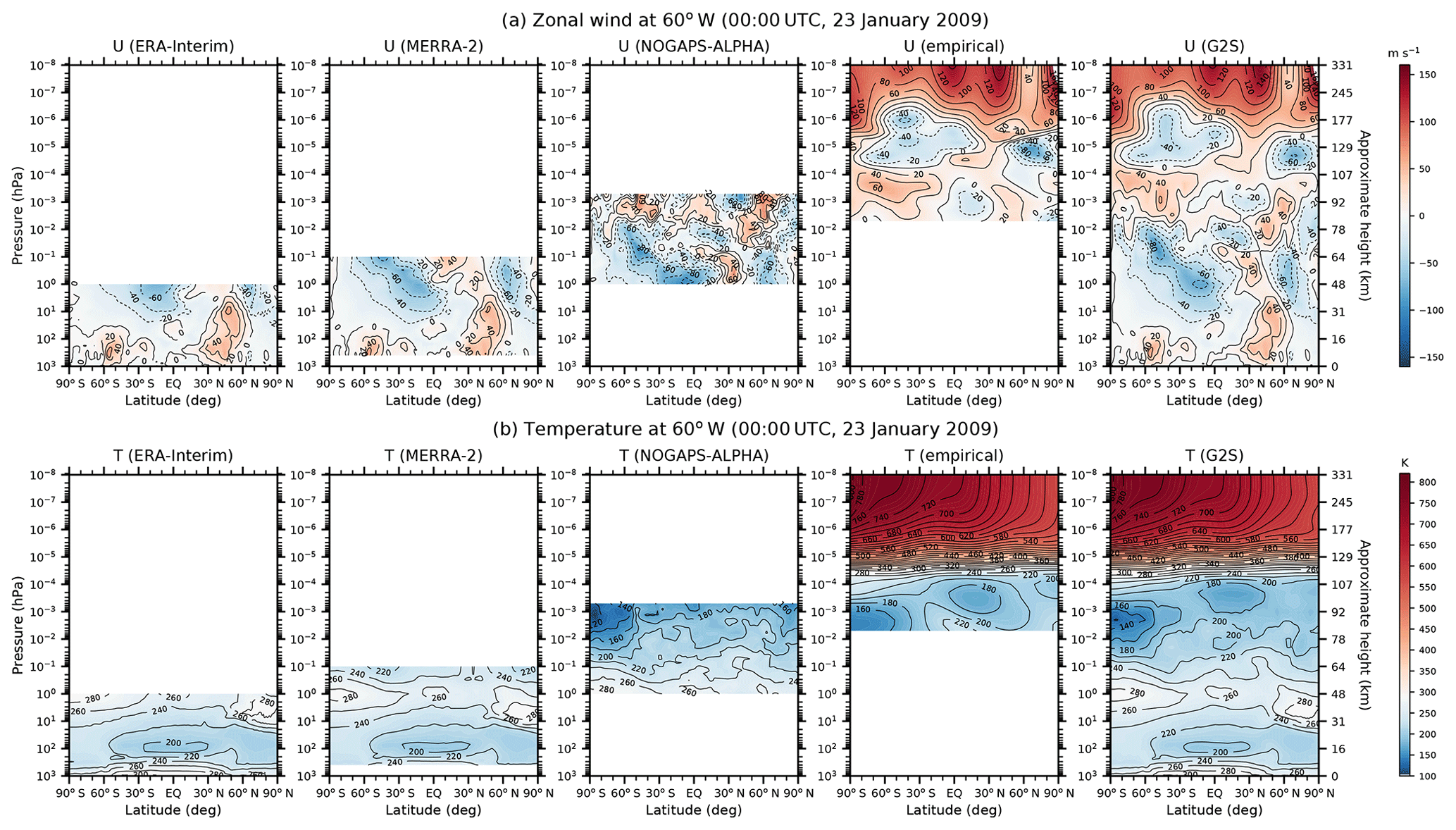
Figure 1Latitude–height cross sections of (a) zonal wind and (b) temperature in the ERA-Interim, MERRA-2, NOGAPS–ALPHA, empirical models, and G2S data at 60∘ W at 00:00 UTC on 23 January 2009. For zonal wind, shading and contour intervals are 2 and 20 m s−1, respectively. Contours for westward winds are plotted in broken lines. For temperature, shading and contour intervals are 5 and 20 K, respectively.
For ray simulations, G2S data at hourly intervals are spatially smoothed using the vertical 1–2–1 smoother and horizontal moving averaging on the spherical surface. Horizontal averaging is done using variables within the area of a spherical cap centered at every latitude–longitude grid point. A spherical cap is defined by an angle between two lines from the sphere center to the center of the spherical cap's surface and to the cap's boundary. The angle is set equal to about 2.7∘, and for this angle, the area of the spherical cap's surface is equivalent to the area of a circle with a radius of 300 km [π(300 km)2] on a flat surface. Smoothed G2S data are regridded at horizontal resolution for use in ray simulations.
In this study, orographic and nonorographic GWs are considered separately. Properties of orographic GWs are given by the M87 scheme. Nonorographic GWs are specified based on SA11 and Warner and McIntyre (1996, hereafter WM96).
4.1 Orographic GWs
Orographic GWs (OGWs) are assumed to be excited when low-level horizontal winds are strong, and vertical parcel displacements, due to subgrid topography, are large (M87).
The vertical displacement (hm) is given by 2σh, where σh is the standard deviation of the subgrid-scale topography. Reynolds stress due to stationary OGWs (ω=0 and cp=0) is given by (kho∕2) ρsNsUs, where kho is the horizontal wave number [], and ρs, Ns, and Us are air density, stability, and horizontal wind magnitude, respectively, averaged within the source layer between the ground and the hm. Grid- and subgrid-scale topography are obtained by averaging and regridding the National Center for Atmospheric Research (NCAR) Community Earth System Model (CESM) auxiliary data with horizontal resolutions close to .
Directions of horizontal wave number vectors are set opposite to horizontal wind vectors averaged within source layer. OGWs are launched at the top of the source layers.
4.2 Nonorographic GWs
For nonorographic GWs (NOGWs), three 14-discrete-wave schemes, as in SA11, are considered. One is a modified version of SA11, and the other two are derived from the empirical spectra of WM96.
The empirical GW energy spectrum () in WM96 is given by a separable function of m, , and the azimuth angle (φ; i.e., ). The pseudomomentum flux spectrum can be written as a function of k, ω, and φ by multiplying the spectrum by the Jacobian factor (). This spectrum is discretized to obtain 14-wave schemes through numerical integrations around appropriately chosen k and ω for 14 sets of φ and cp, as in SA11, in a quiescent atmosphere with a specified stability (0.01 rad s−1). Two 14-wave WM96 schemes are obtained by using two different values (1 and 5∕3) of p in the spectrum given by . NOGWs are launched at every horizontal grid point at z=6.8 km near 400 hPa.
Figure 2 illustrates angular histograms of spectral properties and Reynolds stress in the three 14-wave NOGW schemes. In these schemes, horizontal propagation directions (φs) and ground-based phase speeds (cps) are given for each of 14 GWs, and they are identical to those in SA11. The horizontal wavelength (λh) in SA11 ranges from 385 to 596 km. In WM96 with (WM96a), the range of λh is broader (309–782 km) compared to SA11, and in WM96, with p=1 (WM96b), the range is much broader (128–942 km).
Each GW has an identical amount of Reynolds stress in the three schemes. For this, the stresses for GWs with cp>20 m s−1 are reduced in SA11, and integration intervals of k and ω for the spectra in WM96 are appropriately adjusted. As a result, NOGWs with cps smaller (larger) than 20 m s−1 have Reynolds stress to the order of 10−3 (10−5) N m−2. Reynolds stresses exhibit slightly more westward flux, but they are almost isotropic. The total magnitudes of Reynolds stresses used in this study are N m−2 in the eastward, northward, and southward directions and N m−2 in the westward direction. These magnitudes are comparable to the total momentum flux of N m−2 in each cardinal direction at 450 hPa that is employed in the ECMWF model (Orr et al., 2010). Details of GW properties shown in Fig. 2 are found in Table S1 in the Supplement.
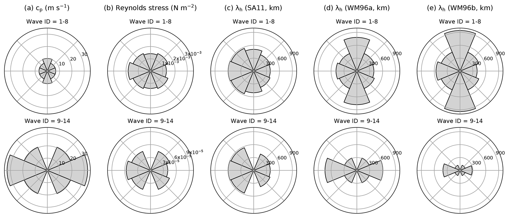
Figure 2Angular histograms of (a) phase speeds, (b) Reynolds stresses, and (c)–(e) horizonal wavelengths of nonorographic GWs (SA11, WM96a, and WM96b) as a function of propagation directions (φ) at an interval of 45∘. For wave IDs of 1–8 (9–14), cp=6.8, 6.8, 10.2, 6.8, 6.8, 6.8, 10.2, and 6.8 m s−1 (32.8, 20.4, 20.4, 32.8, 20.4, and 20.4 m s−1) counterclockwise from due east (φ=0∘).
4.3 Generation of GW ensembles
In ray simulations, a single GW packet, stochastically chosen from GW source ensembles, is launched at a horizontal grid point where GWs are supposed to be generated. This approach is computationally efficient, allowing for statistical significance tests for differences between ray simulations.
The OGW scheme (M87) launches a single OGW at a horizontal grid point, but NOGW schemes usually specify multiple GWs. Hence, GW ensembles are separately generated for OGWs and NOGWs. For OGWs, the vertical displacement hm is assumed to be given by sfσh, where the scale factor sf has a uniform probability distribution between 1 and 3 around its default value 2. For NOGWs, a single GW is selected with uniform chance from 14 discrete waves. GW ensembles are precomputed using a random-number generator for reproducibility.
Figure 3 demonstrates horizontal distributions of zonal OGW and NOGW pseudomomentum fluxes (Fp) at individual launch levels for a particular ensemble member and the ensemble averages of the zonal pseudomomentum fluxes at 00:00 UTC on 20 January 2009, 4 d before the 2009 SSW onset. The stochastic parameters for OGWs and NOGWs are the displacement scale factors (sf) and wave IDs (1–14), respectively. For each of GW source schemes, 20 ensemble members are generated.
For OGWs, sf varies randomly between 1 and 3 at grid points where σh is nonzero. In the midlatitude tropospheric eastward jet regions, westward OGW Fp is large and may reach about −1 N m−2 over major mountainous regions, namely the Alps, the Tibetan Plateau, the Rocky Mountains, and the Andes. Large eastward OGW Fp is found in the higher-latitude regions such as Greenland and Antarctica. Zonal Fp in each OGW ensemble member has locally substantial deviations from the ensemble mean (Fig. 3b) in the major mountain areas. Maximum value of the standard deviation from the ensemble mean is about 0.7 N m−2 and is found in the Tibetan areas.
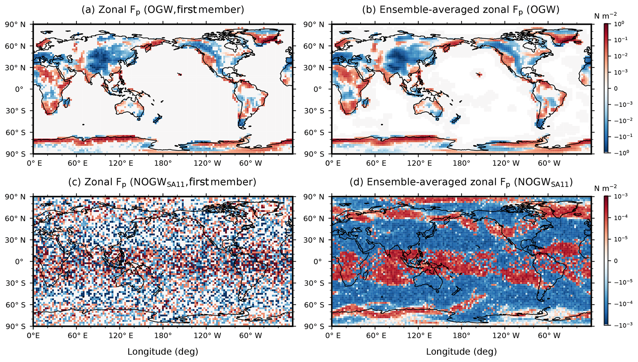
Figure 3Longitude–latitude distributions of zonal pseudomomentum fluxes (Fp) for OGW and NOGWSA11 at 00:00 UTC on 20 January 2009 on the horizontal grid as follows: (a) zonal OGW Fp above source layers for the first OGW ensemble member, (b) ensemble-averaged zonal OGW Fp, (c) zonal NOGW Fp at z=6.8 km for the first NOGW ensemble member, and (d) ensemble-averaged zonal NOGW Fp at z=6.8 km. OGW Fp is multiplied by an efficiency factor (0.125) as described in Richter et al. (2010).
For NOGWs, wave IDs of 1–14 are randomly spread around the globe. The magnitude of ensemble-averaged zonal NOGW Fp is O(10−3 N m−2). The horizontal distribution of zonal Fp in each NOGW ensemble member (Fig. 3c) looks noisy, but characteristic structure is more clearly revealed in its ensemble average (Fig. 3d). The sign of zonal NOGW Fp is generally opposite to that of the tropospheric zonal flows. The organized spatial structure of the zonal NOGW Fp only emerges in the ensemble because any single ensemble member is completely stochastic. Meanwhile, the OGW Fp is well organized in a single ensemble member because they are constrained by the OGW source parameterization that depends explicitly on orography.
GW ray simulations are carried out for the time period of 25 d from 00:00 UTC on 8 January 2009 to 00:00 UTC on 2 February 2009 for the 20 OGW and NOGW ensemble members.
For each GW ensemble member, two kinds of simulations are carried out, namely four-dimensional (4D; x–z and t) and two-dimensional (2D; z and t) experiments. In the 4D experiments, GW rays propagate horizontally and vertically in spatially varying background media, but in the 2D, rays are allowed to propagate only in the vertical direction. In both the 4D and 2D, GW rays propagate through time-varying flows, and therefore modulations of the observed frequencies of GWs occur. In the 4D cases for M87 and SA11, additional simulations where τdef=0 in the amplitude equation are carried out to see ray-tube effects. In all simulations, 3 h averaged gridded outputs are generated. GW rays are launched every 3 h, and 3 d old rays are eliminated. These launch intervals and ray lifetimes are chosen considering computational time, the timescale of the large-scale flow, and elapsed time for rays launched in the troposphere to reach the upper mesosphere and lower thermosphere (UMLT; see Figs. S1–S3).
5.1 Zonally averaged GW properties
Figure 4 shows latitude–height distributions of zonal mean zonal wind and ensemble averages of zonal mean zonal Fp of OGWs and three NOGWs in the 4D and 2D experiments at 00:00 UTC on 20 January 2009. The NH polar vortex is not reversed but is much weakened. Hatched areas indicate regions where differences between the 4D and 2D are not statistically significant. The signs of the zonal mean zonal pseudomomentum fluxes below z=80 km are similar overall in the 4D and 2D and seem to be related to the structure of the zonal wind, but they become different from each other above z=80 km in the NH polar regions.
Statistically significant differences between the 4D and 2D are found in five regions. (i) In the latitude–height region of 40–70∘ N and 40–50 km, westward Fp in the 4D is enhanced about 10 times when compared with the 2D results for OGW, NOGWSA11, and NOGWWM96a, and they are about 28 times increased when compared with the 2D results for NOGWWM96b. (ii) In the NH polar UMLT (70–80∘ N and 85–100 km), the magnitude of eastward Fp in the 4D is 1.5–5 times larger than that of westward Fp in the 2D for both OGWs and NOGWs. This result implies that the 4D results may better explain the mesospheric cooling around the SSW central dates, compared to the 2D, given that the cooling can be induced by eastward GW momentum forcing in the UMLT. (iii) In the upper troposphere and lower stratosphere (UTLS) above the tropospheric jets, westward Fp of NOGWs is 1.6–2.6 times larger in the 4D. (iv) In the SH mesosphere, eastward Fp of NOGWs in the midlatitudes is reduced by more than half in the 4D. (v) Eastward Fp of OGWs at z=30–80 km around 70∘ S is enhanced 5–6 times in the 4D. As a result, the magnitude of zonal Fp in the middle atmosphere and its structure in the UMLT can be substantially changed in the 4D where horizontal propagation and refraction are allowed, even though Fp is given identically at source levels in the 4D and 2D experiments.
Additional 4D OGW and NOGWSA11 experiments (Fig. S4) where no ray-tube effects are considered (τdef=0) give similar results to those with τdef≠ 0 shown in Fig. 4, except for the NH upper stratosphere and lower mesosphere (USLM). Statistically significant differences between nonzero and zero τdef are found in relatively narrow regions around the NH jet core (75∘ N and 40 km at 00:00 UTC on 20 January 2009; see Fig. S4). It is interesting that ray-tube effects become important in regions near the jet where the large-scale winds vary rapidly in space (see Sect. 5.2). In these regions, the magnitude of westward Fp when τdef≠0 is reduced by less than half compared to when τdef=0. These differences are localized compared to the differences between the 4D and 2D experiments, which may indicate that ray-tube effects are relatively limited. However, it should be noted that ray simulations in this study may underestimate ray-tube effects, given that horizontal spread of GW fields that emanate from local sources cannot be considered in the current ray simulations where a single GW ray is launched at a grid point.

Figure 4Latitude–height cross sections of (a) zonal mean zonal wind (ZU) and (b–i) zonal mean zonal pseudomomentum fluxes (Fp) for OGW and three NOGW schemes in the (top row) 4D and (bottom row) 2D experiments at 00:00 UTC on 20 January 2009. OGW Fp is multiplied by the efficiency factor (0.125). Contour interval of zonal mean zonal wind is 10 m s−1, and negative values are plotted in broken lines. Hatched areas on the pseudomomentum fluxes indicate regions where the paired and two-tailed t test for 20 ensemble members of the 4D and 2D experiments give p values larger than 0.05 (i.e., no statistical significance at the level of 0.05). Here, the p value means there is a probability that mean values in the 4D and 2D experiments would be similar to each other. The hatched areas are identical in the pair of 4D and 2D experiments for a particular GW scheme. A non-parameteric test, such as Wilcoxon's signed rank test, where no probabilistic distribution is assumed, also gives almost similar results to the t test. For these statistical tests, algorithms presented in Boslaugh (2013) are employed.
Figure 5 shows latitude–height distributions of zonal mean zonal wind and ensemble means of zonally averaged zonal wave numbers (k) for OGWs and NOGWs in the 4D and 2D experiments at 00:00 UTC on 20 January 2009. It is clear that the sign of zonal mean k is overall the same as that of the zonal Fp shown in Fig. 4, except for some regions in the NH USLM. This similarity in the signs of k and zonal Fp implies that the zonal mean zonal Fp (Fig. 4) is mostly due to upward-propagating GWs, since the sign of zonal Fp (=kFA) is determined by the sign of k alone in case that cgz> 0 and thus FA> 0. In the NH USLM, however, GWs in the 4D are found to propagate downward in some areas, and positive k at z=30–50 km is related to the GWs with negative cgz and westward Fp (see Sect. 5.2 for details).
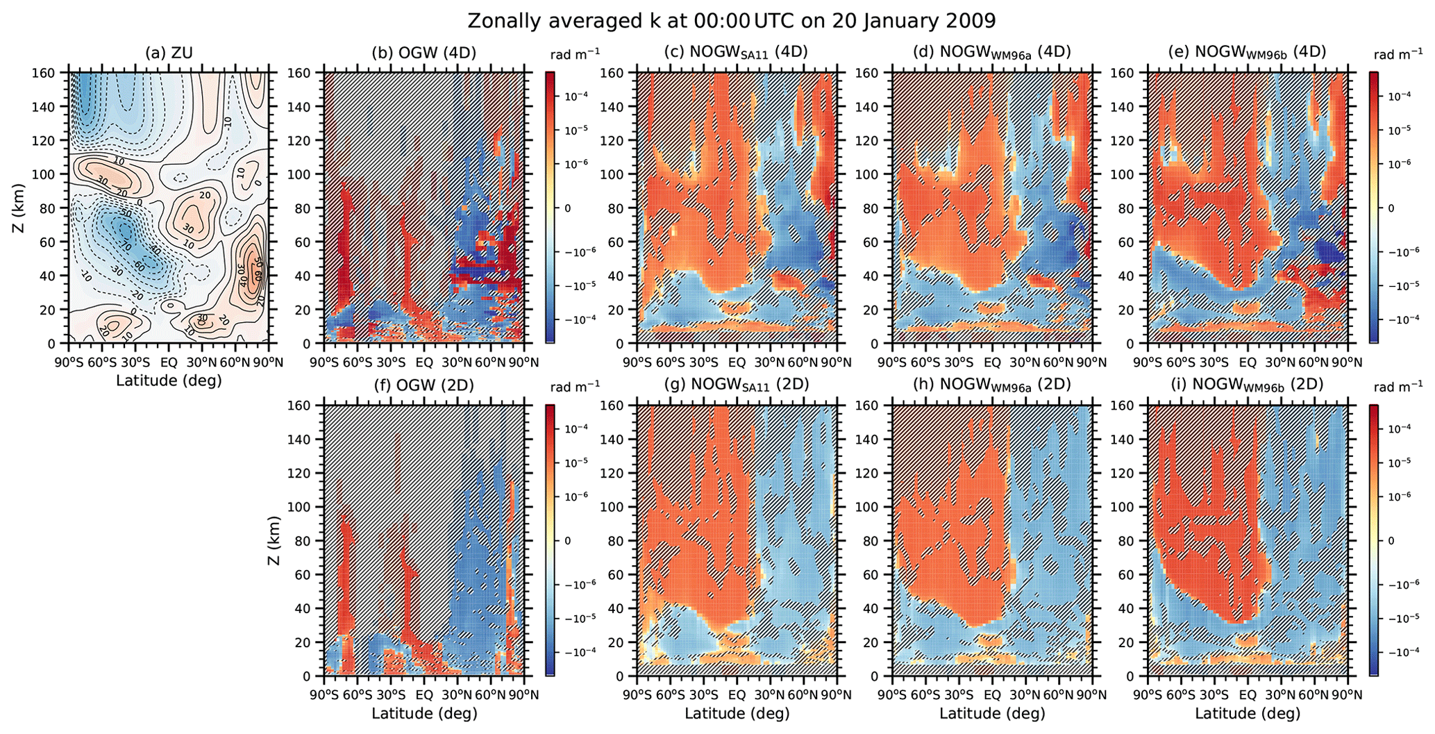
Figure 5Latitude–height cross sections of (a) zonal mean zonal wind (ZU) and (b–i) zonal mean zonal wave numbers (k) for OGW and three NOGW schemes in the 4D and 2D experiments at 00:00 UTC on 20 January 2009. Contour interval of zonal mean zonal wind is 10 m s−1 and negative values are plotted in broken lines. Hatched areas on the zonal wave numbers indicate regions where the paired and two-tailed t test for the 4D and 2D experiments gives p values larger than 0.05 (i.e., no statistical significance at the level of 0.05).
Statistically significant differences of zonal mean k between the 4D and 2D are also found in similar regions to those of zonal mean zonal Fp shown in Fig. 4. In the NH polar UMLT, the sign of k is reversed between the 4D and 2D, and the magnitude of positive k in the 4D is 1.2–6.3 times larger than that of negative k in the 2D for both OGWs and NOGWs. In the UTLS, negative k of NOGWs is 1.4–2.4 times larger in the 4D. In the SH mesosphere, positive k of NOGWs in the midlatitude regions is reduced by about half in the 4D, and positive k of OGWs around 70∘ S is enhanced about 1–3 times in the 4D. These changes in k in the 4D with respect to the 2D are roughly similar to those in the zonal Fp shown in Fig. 4. This result indicates that differences in the zonal Fp between the 4D and 2D experiments can be accounted for to a substantial degree by changes in the k between the 4D and 2D.
The time rate of change of k along rays is determined by the five forcing terms (Eqs. A13 and A17). Among the five terms, the two zonal shear forcing terms [ and ] and curvature term (lcgλtan ϕ∕a) are predominant in most cases. The other forcing terms in Mλ∕hλ (Eq. A17) that depend on the stability (N2) and vertical density variation (α2) are usually 2–3 orders of magnitude smaller (see Fig. S5).
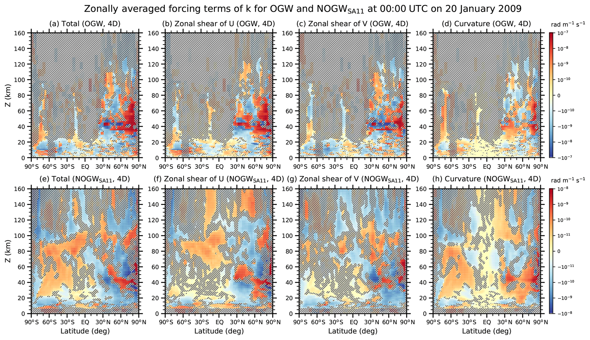
Figure 6Latitude–height cross sections of total and three major forcing terms – the zonal shear terms of the large-scale zonal and meridional winds (U and V) and the curvature term – of the zonal wave number for (top row) OGW and (bottom row) NOGWSA11 in the 4D experiment at 00:00 UTC on 20 January 2009. The zonal shear terms of U and V are and , respectively. The curvature term is given by lcgλtan ϕ∕a. Hatched areas indicate regions where the paired and two-tailed t test for the 4D and 2D experiments gives p values larger than 0.05 (i.e., no statistical significance at the level of 0.05).
Figure 6 shows latitude–height distributions of the total and three major forcing terms in the k equation for OGWs and NOGWSA11's in the 4D experiment at 00:00 UTC on 20 January 2009. Note that the forcing terms in the k equation in the 2D are all zero. For NOGWs, results for SA11 are presented since the other NOGW schemes give roughly similar results. It is clear that the magnitude of the curvature term is as large as the two zonal shear forcing terms in the midlatitudes as well as the polar regions, which supports the importance of the curvature term presented by Hasha et al. (2008). In the UTLS, the total forcing term for NOGWs is generally negative above the tropospheric jet cores (60–40∘ S and 20–50∘ N) where the negative k is predominant and enhanced in the 4D, and the negative total forcing is mainly due to the zonal shear term of zonal winds and curvature effects. For OGWs around 70∘ S, the enhancement of the positive k in the stratosphere is attributed to curvature effects. For NOGWs, curvature effects are predominant over the other two major forcing terms in the SH stratosphere where winds are steady, but they are a little smaller than the two zonal shear forcing terms in the NH where the polar vortex varies rapidly in space and time.
The structure of the three major forcing terms in the k equation (Fig. 6) is different from that of k (Fig. 5), except for the NH USLM. This difference may occur in relation to space and time propagation of GWs, since certain k's substantially changed in some regions may not be changed a lot as GWs propagate to the other regions. In fact, positive k of NOGWs with eastward Fp in the UTLS of the SH mid- to high-latitude regions is increased by positive zonal shear terms for the zonal wind and curvature terms (Fig. S5). The increase in positive k enhances eastward Fp in the SH UTLS. However, the eastward Fp of NOGWs is reduced in the SH middle atmosphere, even though total forcing in the k equation for NOGWs with eastward Fp is positive (Fig. S5). It is seen that the GWs with enhanced eastward Fp would be dissipated through the saturation as they propagate northward toward the SH midlatitude USLM. This dissipation results in reduction in eastward Fp and positive k in the SH mesosphere (Figs. 4–5). In contrast, distributions of k and major forcing terms (Fig. 6) are correlated with each other in the NH USLM, which indicates that the structure of k in the NH USLM can be locally generated by forcing terms around z=40 km.
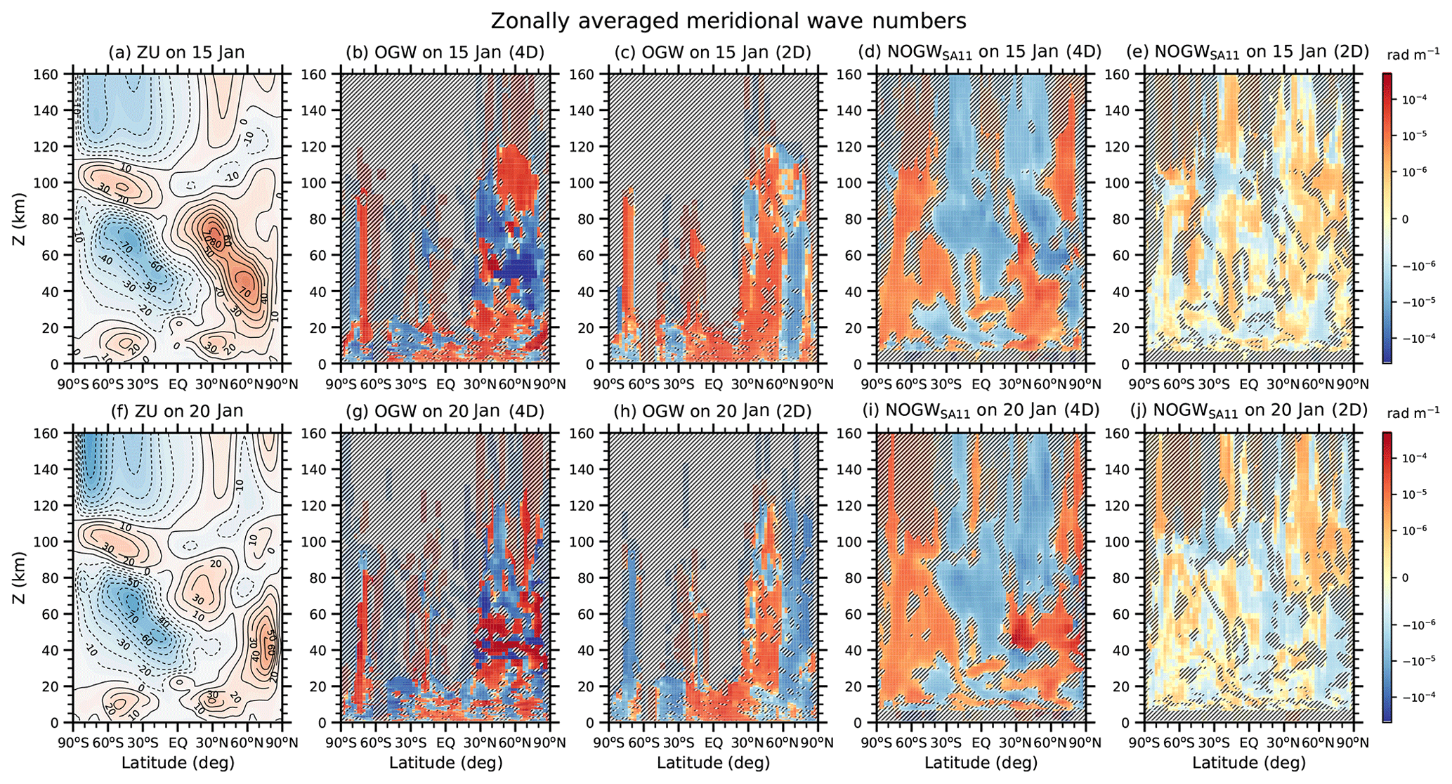
Figure 7Latitude–height cross sections of zonal mean zonal wind (ZU) and ensemble means of zonally averaged meridional wave numbers (l) for OGW and NOGWSA11 in the 4D and 2D experiments at 00:00 UTC on (top row) 15 and (bottom row) 20 January 2009. Contour interval for zonal mean zonal wind is 10 m s−1, and negative values are plotted in broken lines. Hatched areas on the meridional wave numbers indicate regions where the paired and two-tailed t test for the 4D and 2D experiments gives p values larger than 0.05 (i.e., no statistical significance at the level of 0.05).
Figure 7 shows latitude–height distributions of zonal mean zonal wind and ensemble means of zonally averaged meridional wave numbers (l) for OGWs and NOGWSA11's in the 4D and 2D experiments at 00:00 UTC on 15 and 20 January 2009. It is found that the structural difference of l between the 4D and 2D is substantial for both OGWs and NOGWs and is more significant than the difference in structure of k. This result may be related to larger meridional variations of the large-scale flow than its zonal variations, given that the time rates of changes of l and k are determined by meridional and zonal variations of the large-scale flow, respectively.
In the SH, large positive l of OGWs appears around 70∘ S in the 4D compared with the 2D on both of the two dates, and these are due to the positive meridional shear forcing term related to zonal wind [], where k>0, and (see Fig. S6). In the NH USLM, positive (negative) l of OGWs in the 4D appears roughly south (north) of the eastward jet axis on 15 January but significantly enhanced positive l is predominant on 20 January. The signs of l across the jet on 15 January mean northward (southward) propagation of OGWs relative to large-scale meridional winds. Therefore, OGWs in the 4D can in fact be converged along the jet axis in the NH USLM, as long as the meridional variations of meridional winds are not significant. On 20 January, as the jet is moved towards 80∘ N, it is seen in the 4D that positive l of OGWs and poleward propagation of OGWs become predominant south of the jet axis. In the 2D, the structure of l of OGWs in the NH does not seem to exhibit significant responses to spatiotemporal variations of the large-scale flow.
The structure of l for NOGWs is coherent with the large-scale flow structure in the 4D, but it seems more or less random in the 2D. In the SH, l of NOGWs in the 4D is positive overall in the high-latitude stratosphere above z=10 km and in the midlatitude middle atmosphere above z=30 km, and cgλ is negative overall due to the westward winds. This explains why the curvature term (lcgλtan ϕ∕a) in the k equation is positive for NOGWs in the SH (ϕ<0) middle atmosphere, as shown in Fig. 6h. The positive l of NOGWs in the SH is mainly due to the forcing term related to the meridional shear of zonal winds and curvature term () in the l equation (see Fig. S6). Positive k above z=40 km (Fig. 5) and changes in the sign of around the axis of the westward winds ( south of the axis and north of the axis) make the meridional shear forcing term in the l equation positive in the SH polar USLM and negative in the SH midlatitude USLM. In the NH USLM, as in OGWs, the structure of the l on 15 January may indicate latitudinal convergence of NOGW rays along the axis of the stratospheric jet. On 20 January, positive l is predominant in the NH USLM, and NOGWs south of 80∘ N propagate northward.

Figure 8 shows latitude–height distributions of zonal mean zonal wind and ensemble means of the zonally averaged number of GW packets for OGWs and NOGWSA11's in the 4D and 2D experiments at 00:00 UTC on 15 and 20 January 2009. The number of GW packets corresponds to the ray counter used for averaging in the gridding method. Comparison between the 4D and 2D indicates that there is convergence of GW packets in the 4D along the jet axis in the NH USLM and in the NH polar stratosphere on 15 January for both OGWs and NOGWs. In the latitude–height region of 40–70∘ N and 40–90 km on 15 January, the zonally averaged number of rays for OGWs (NOGWs) is about 0.9 (1.9) in the 4D, and it is 1.7 (1.3) times larger than in the 2D. In this region, GWs with westward Fp outnumbers GWs with eastward Fp, and therefore the ray convergence may increase the westward Fp. In the NH, mid- to high-latitude lower thermosphere (30–90∘ N and 120–140 km), the zonally averaged number of rays for OGWs (NOGWs) is about 2.5 (1.9) times larger in the 4D on 15 January. This difference is mainly due to OGWs and NOGWs with eastward Fp (not shown).
As the eastward jet in the stratosphere moves towards the North Pole on 20 January, the number of GW packets in the 4D increases in the NH polar mid- to upper stratosphere (50–80∘ N and 30–50 km). In this region, the zonally averaged number of rays for OGWs (NOGWs) is about 0.9 (2.3) in the 4D, and it is 1.7 (1.1) times larger than in the 2D. As on 15 January, GWs with westward Fp are predominant in the NH stratosphere, resulting in some enhancement of westward Fp. In the NH lower thermosphere (30–90∘ N and 120–140 km), the zonally averaged number of rays for both OGWs and NOGWs is about 1.8 times larger in the 4D. This increase is mostly attributed to OGWs and NOGWs with eastward Fp, as on 15 January.
GWs generally propagate more to the thermosphere in the 4D. Even though the eastward winds are still large in the NH middle atmosphere on 15 and 20 January, both OGWs and NOGWs with eastward Fp (i.e., k> 0 and , where cpλ is the ground-based zonal phase speed) can propagate better to the thermosphere in the 4D since they are less dissipated in the middle atmosphere. There seems to be a tendency in the 4D for GWs to elude critical-level filtering or nonlinear saturation better in the lower atmosphere. This tendency may be attributed to a larger degree of freedom in propagation associated with change in wave number directions due to refraction and curvature effects that can occur before either filtering or saturation is initiated as GWs approach critical levels. Similar results can also be found for NOGWs in the SH. More NOGW packets in the 4D are found in the SH middle atmosphere, and they are related to reduced restriction in the propagation of GWs with eastward Fp towards the middle atmosphere. Also, as GWs propagate better toward the upper atmosphere, GW packets (with eastward Fp) in the 4D look vertically more spread near z=90 km in the SH where the zonal mean zonal wind is reversed. This spread in the 4D compared to the 2D implies that GWs in the 4D may better avoid filtering without being trapped in a narrow vertical layer close to critical levels.
Convergence (or focusing) of GW packets may have some effects on distribution of the GW pseudomomentum fluxes. Song and Chun (2008) emphasized this effect as an important mechanism that accounts for differences between ray-based and columnar GWPs. Discussion regarding Fig. 8 indicates that convergence or divergence (spread of GW packets) effects in the 4D would be smaller than a factor of 2 in terms of the magnitude of Fp. These convergence and divergence effects are, however, likely relatively small compared to impacts due to change in horizontal wave numbers shown in Figs. 4–5, although the refraction effects would not entirely lead to local change in mean flows (see Sect. 5.2).
The spatial distribution of GW packets in the 4D is generally more contiguous in the latitudinal direction than that in the 2D in which latitudinal discontinuity is clear. This difference indicates more than improvement in the smoothness of the GW pseudomomentum fluxes in the 4D. Since McLandress and McFarlane (1993), various modeling studies have suggested that PW momentum forcing tends to be compensated by parameterized GW momentum forcing. Cohen et al. (2013) noted that the GW momentum forcing on small latitudinal scales can induce instability that generates PWs to be involved in the compensation. Given that the latitudinal discontinuity of the pseudomomentum fluxes in the 2D is unrealistic compared to the 4D, the discontinuity due to columnar GWPs can possibly generate spurious PWs in models. Therefore, it cannot be said that compensation between PW and GW forcing always occurs for the right reasons in models with columnar GWPs. For further understanding of the compensation, the 4D formulation beyond columnar GWPs can be required because change in the GW pseudomomentum due to the horizontal refraction can induce change in mixing of the mean potential vorticity (PV) around an aggregate of the refracted GWs. This GW-induced PV mixing can produce changes in PW-induced PV mixing in the surf zone related to PW breaking, resulting in compensation between PW and GW effects (Cohen et al., 2014).
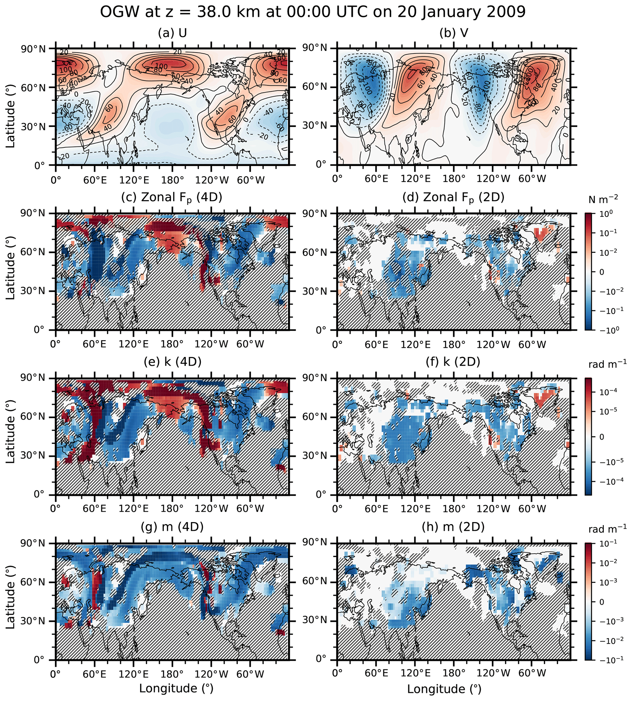
Figure 9Longitude–latitude cross sections of (a) zonal wind (U), (b) meridional wind (V), and ensemble means of (c–d) zonal pseudomomentum fluxes (Fp), (e–f) zonal wave numbers, and (g–h) vertical wave numbers for OGW at z=38 km in the 4D and 2D experiments at 00:00 UTC on 20 January 2009. OGW Fp is multiplied by the efficiency factor (0.125). Contour interval for zonal and meridional winds is 20 m s−1, and negative values are plotted in broken lines. Hatched areas indicate regions where the paired and two-tailed t test for the 4D and 2D experiments gives p values larger than 0.05 (i.e., no statistical significance at the level of 0.05).
5.2 Horizontal distributions of GW characteristics
Figure 9 shows longitude–latitude distributions of zonal and meridional winds and ensemble averages of zonal pseudomomentum fluxes (Fp) and zonal and vertical wave numbers (k and m) for OGWs at z=38 km in the 4D and 2D experiments at 00:00 UTC on 20 January 2009. Zonal and meridional winds demonstrate that PWs of zonal wave number 2 (ZWN2) are significantly enhanced in the NH stratosphere. The PWs are accompanied by large spatial gradients of horizontal winds in the NH mid- to high-latitude regions. As shown in the previous section, zonal Fp and k can be significantly changed in association with zonal gradients of horizontal winds.
The horizontal structure of zonal Fp is significantly different between the 4D and 2D. First of all, zonal Fp of OGWs in the 4D is widespread in the NH mid- to high-latitude regions, and it is significantly enhanced in some particular areas where large zonal gradients of horizontal winds appear. In the 4D, nonzero zonal Fp is newly found over western Europe, the north of northern Europe, the north of the Kamchatka Peninsula, the west of North America, and over Greenland. This regional difference in nonzero zonal Fp indicates the effects of horizontal propagation. In polar regions and west of North America, zonal Fp of OGWs is directed eastward in the 4D. This eastward Fp is related to positive k induced by refraction or curvature effects. In the 2D, eastward Fp of OGWs appears only over Greenland where Fp is eastward from launch levels.
The increase in the magnitudes of zonal Fp and k appears together in narrow areas between southward and northward winds (80∘ E and 80–140∘ W around 30–70∘ N), between westward and eastward winds (20–60∘ E and 30∘ N), and along the polar eastward jets. This enhancement is spatially correlated with the two zonal shear forcing and curvature terms in the k equation (not shown), and therefore it is thought of as being locally induced by the wind shear and curvature terms. In these narrow areas, the magnitudes of k and m become O(10−4–10−3 rad m−1) and O(10−2–10−1 rad m−1), respectively. That is, zonal and vertical wavelengths can be as small as O(1–10 km) and O(10–100 m), respectively. In some areas between southward and northward winds (60∘ E and 130∘ W), m is positive (i.e., cgz<0), positive k is large, and as a result, westward Fp is enhanced. This situation shows that large increases in Fp can occur locally as GWs propagate downward, experiencing substantial horizontal refraction.
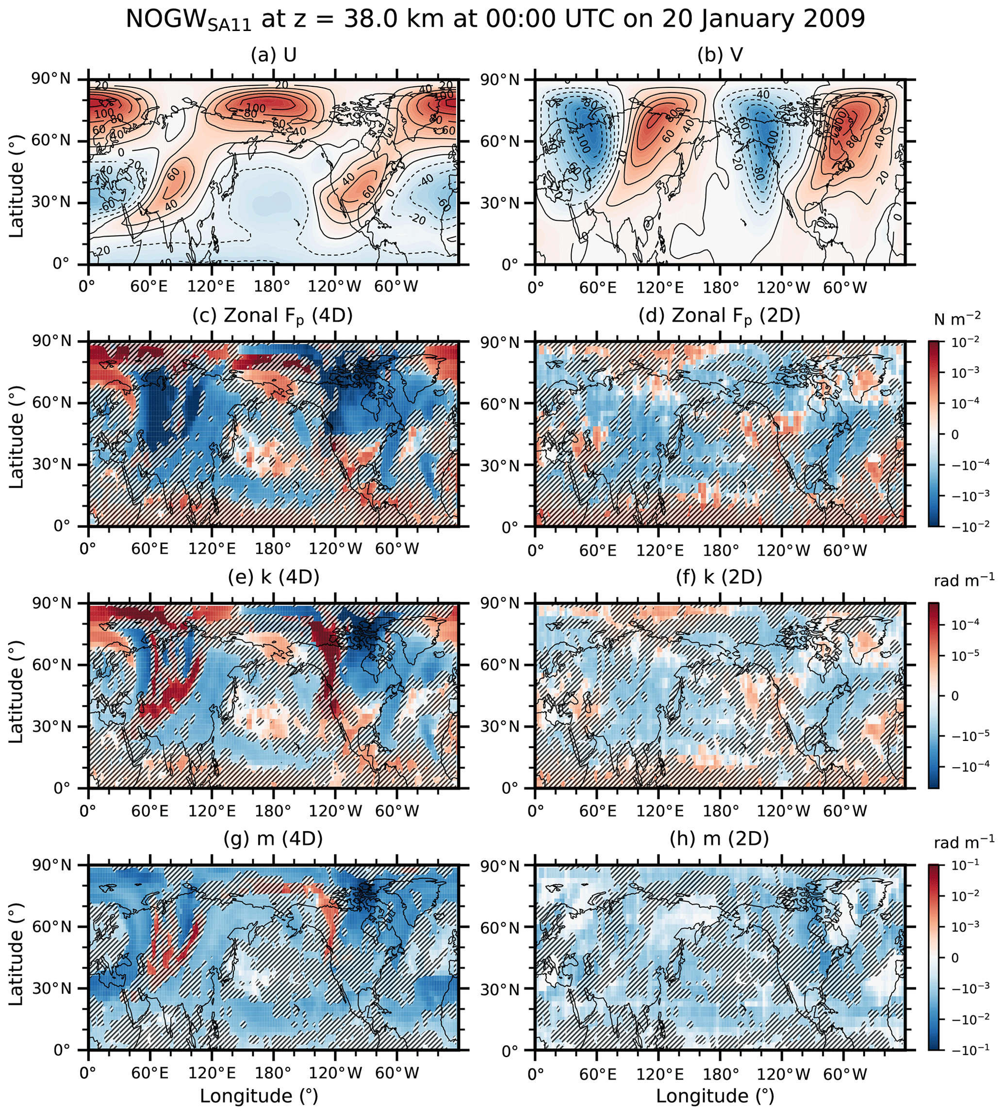
Figure 10Same as Fig. 9 except for NOGWSA11.
Horizontal distributions of zonal Fp, k, and m for NOGWSA11's at z=38 km at 00:00 UTC on 20 January 2009 (Fig. 10) can also be accounted for in similar ways as in the case of OGWs shown in Fig. 9. Statistically significant differences in zonal Fp between the 4D and 2D are mostly found in the NH mid- to high-latitude regions. Similar to OGWs, zonal Fp of NOGWs is significantly enhanced in regions where the zonal gradients of horizontal wind components and curvature effects are large (not shown). Enhancement of westward Fp near 60∘ E (north of Canada) is largely due to the zonal shear term of zonal (meridional) winds. Along narrow regions where large zonal gradients of meridional winds appear (Fig. 10b), positive k is substantially increased, m is positive (i.e., cgz<0), and as a result, zonal Fp is directed westward. In these regions, westward Fp becomes significantly large, and zonal and vertical wavelengths of NOGWs can also be O(1–10 km) and O(10–100 m), respectively, owing to horizontal refraction related to the zonally varying meridional wind.
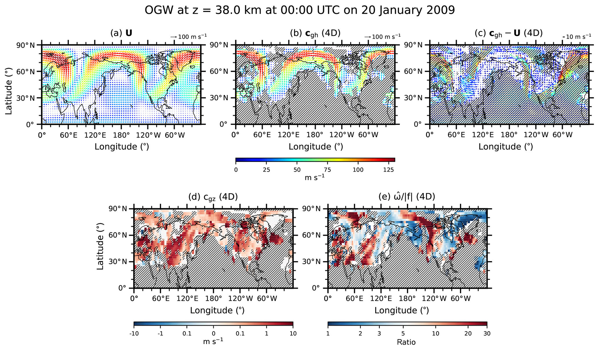
Figure 11Longitude–latitude cross sections of (a) horizontal wind (U), ensemble means of (b) the horizontal group velocity (cgh), (c) the horizontal intrinsic group velocity (cgh−U), (d) the vertical component of the group velocity (cgz), and (e) ratio of intrinsic frequency () to Coriolis parameter () for OGW at z=38 km in the 4D experiment at 00:00 UTC on 20 January 2009. Hatched areas indicate regions where the paired and two-tailed t test for the 4D and 2D experiments gives p values larger than 0.05 (i.e., no statistical significance at the level of 0.05). For hatching over horizontal vector fields (b–c), the mean value of p values for the zonal and meridional components is used.
Figure 11 shows longitude–latitude distributions of horizontal wind velocity (U) and ensemble averages of the horizontal group velocity (cgh), horizontal intrinsic group velocity (cgh−U), vertical component of the group velocity (cgz), and ratio of intrinsic frequency to Coriolis parameter () for OGWs at z=38 km in the 4D experiment at 00:00 UTC on 20 January 2009. Distributions of the horizontal group velocity and horizontal wind velocity look similar to each other, but in fact they exhibit clear differences as shown in the intrinsic group velocity.
Over the Tibetan Plateau and Rocky Mountains, the horizontal intrinsic group velocity is not close to zero. Therefore, in these regions, OGWs propagate relative to the horizontal winds. Meanwhile, in the meridionally elongated regions near 60∘ E, 130∘ W, and 100–140∘ E; in the zonally elongated regions around the longitude of 180∘ between 60 and 80∘ N; and in isolated regions near (60∘ N, 160∘ W), (50∘ N, 90∘ W), and (70∘ N, 60∘ W), the magnitude of the horizontal intrinsic group velocity is roughly close to zero (see white areas in Fig. 11c). Therefore, OGW packets roughly move at the large-scale horizontal wind velocity in these areas. That is, OGW packets behave like tracers advected by the horizontal winds. The stratospheric jets (Fig. 11a) meander around these regions, but the jet cores are somewhat displaced with respect to the regions except for the meridionally elongated regions near 60∘ E and 130∘ W. Vertical group velocity components (cgz) are at least 1 order of magnitude smaller than the magnitude of the horizontal intrinsic group velocity [O(1–10 m s−1)] in these elongated and isolated regions. In regions near (60∘ N, 160∘ W), (70∘ N, 60∘ W), and (60∘ N, 60∘ E) among the regions of the small horizontal intrinsic group velocity, cgz is particularly close to 0. Relatively large positive cgz of O(1–10 m s−1) are found near 120 and 40∘ W, 20–40∘ E, and 80–100∘ E. These regions are roughly found in the peripheries of the regions of the small horizontal intrinsic group velocity.
Equation (13) shows the magnitude of the 3D intrinsic group velocity as a function of wave numbers and intrinsic frequency under the Boussinesq approximation (m2≫α2) as follows:
where κ is the magnitude of the 3D wave number vector (). From Eq. (13), it is clear that the magnitude of the intrinsic group velocity approaches zero in case κ significantly increases.
It is already seen that the magnitude of zonal and vertical wave numbers (Fig. 9) are substantially increased in the narrow and elongated regions around 60∘ E and 130∘ W and along the axis of the polar eastward jets. In these regions, (cgλ, cgϕ) ≈ (U, V) as shown in Fig. 11. For small , intrinsic frequency need not be necessarily small (Eq. 13), although the ratio approaches the limiting value () as the magnitude of the wave number approaches infinity (Bühler, 2014). The ratios, in fact, have a broad range of values in the regions of the small . The ratios are quite small (1–2) over the west of Greenland and the west of Alaska, but they are quite large (10–20) along 130∘ W east of Alaska and the north of western Russia.
The significant enhancement of zonal Fp (=kcgzA) in the elongated areas along 60∘ E and along 80∘ N around the longitude of 180∘ implies an increase in zonal GW pseudomomentum (kA) since cgz's are not particularly increased. Increases in the zonal pseudomomentum in these regions where the intrinsic group velocity is quite small indicates that there is a possibility of occurrence of the wave capture (Bühler and McIntyre, 2005) in the elongated areas during the evolution of the SSW event. When is small in the highly strained large-scale flow, GW packets behave like tracers, and their shape is also substantially stretched, which leads to an increase in wave numbers and thus pseudomomentum. For GW packets in slowly varying mean flows, the change in the pseudomomentum should be balanced by a change in a quantity called impulse, defined by the mean flow vortex structure away from GW packets, unless there are external forces (Bühler, 2014). Hence, the enhanced pseudomomentum of GWs captured by distorted mean flows can cause a change in vortical motions far from GW packets. However, the surged pseudomomentum in the narrow areas may not lead to significant local change in mean flows even when the GWs are dissipated, as described by Bühler (2014).
As shown in Figs. 4–5, zonally averaged eastward Fp in the NH UMLT is enhanced in the 4D, and it is related to positive k. At z=92 km, differences in zonal Fp of NOGWs between the 4D and 2D appear over broad longitudes in the NH polar region north of 60∘ N (Fig. S7). In the 4D, eastward Fp in the NH polar region is correlated with positive k, and m's are negative (cgz>0). The positive k is not locally induced by zonal shear or curvature terms near z=92 km (not shown), and it seems to be gradually acquired as NOGWs propagate upward through the middle atmosphere.
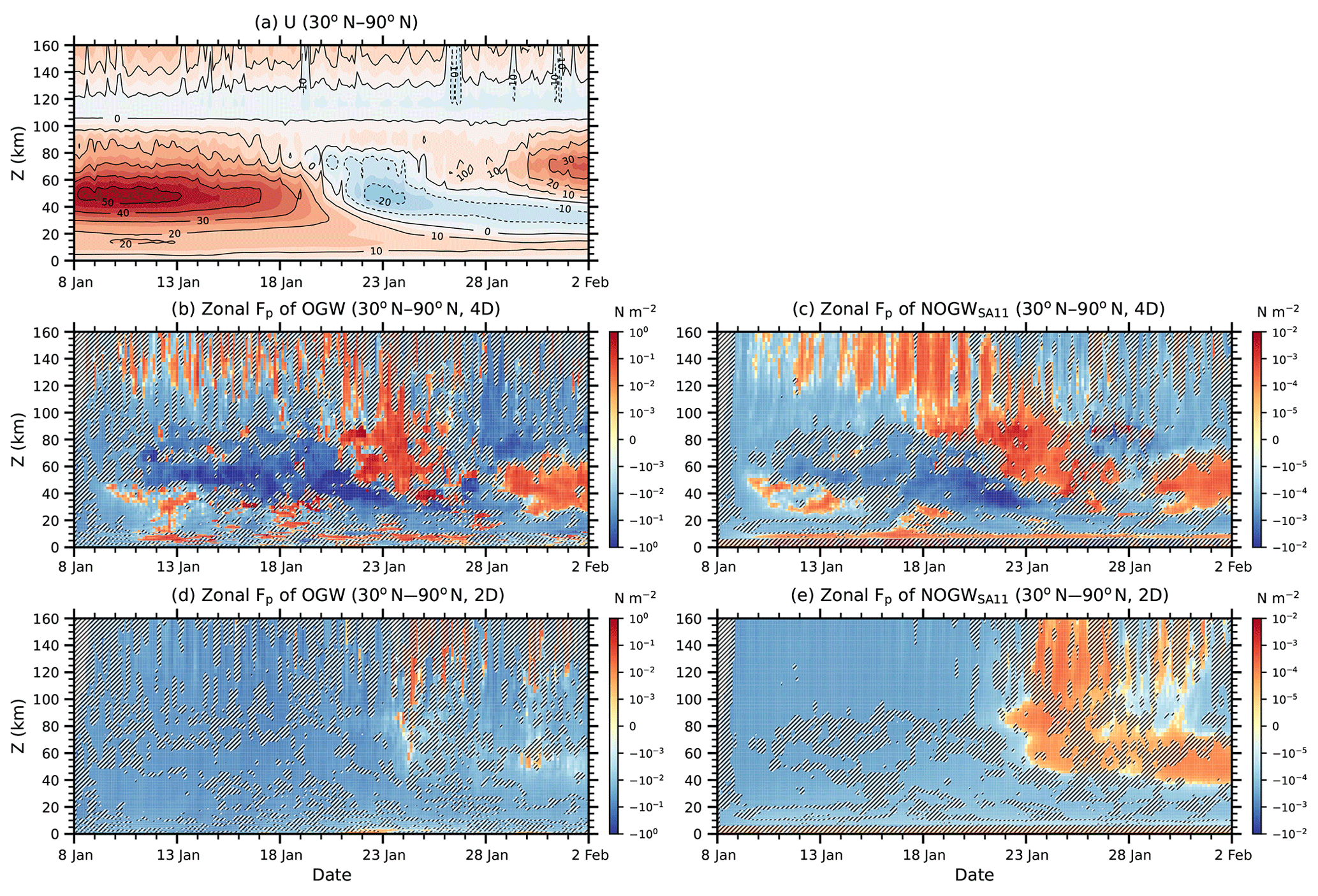
Figure 12Time–height cross sections of (a) zonal wind (U), and (b–e) ensemble means of zonal pseudomomentum fluxes (Fp) averaged over 30–90∘ N for OGW and NOGWSA11 in the (top row) 4D and (bottom row) 2D experiments. OGW Fp is multiplied by the efficiency factor (0.125). Contour interval for zonal winds is 10 m s−1, and negative values are plotted in broken lines. Hatched areas over the zonal Fp indicates regions where the paired and two-tailed t test for the 4D and 2D experiments give p values larger than 0.05 (i.e., no statistical significance at the level of 0.05).
5.3 Time variations of pseudomomentum fluxes
Figure 12 shows time–height cross sections of zonal mean zonal wind and ensemble averages of zonal Fp of OGWs and NOGWSA11's averaged between 30 and 90∘ N in the 4D and 2D experiments from 8 January to 2 February 2009. Time–height distributions of zonal Fp are also quite different between the 4D and 2D. First, westward Fp in the 4D is significantly enhanced in the upper stratosphere from 13 January, about 10 d before the onset date (24 January). Increase of westward Fp is larger in OGWs than in NOGWs. Second, there is larger eastward Fp of OGWs and NOGWs in the middle stratosphere (z=30–40 km) and lower thermosphere (z=120–160 km) in the 4D from the early stage of the SSW evolution. Third, eastward Fp is substantially enhanced in the upper mesosphere a few days earlier than the onset date in the 4D. Fourth, eastward Fp of OGWs is increased in the 4D in the USLM around z=40 km in the recovery phase after the onset.
Enhanced westward Fp in the upper stratosphere before onset is clearly related to the surge of pseudomomentum associated with GWs captured by vortical mean flows. The other enhancements in the magnitude of zonal Fp in the 4D, however, do not seem to be related to the wave capture, and they are likely due to GWs in the 4D that propagate upward better, avoiding filtering or saturation in the lower atmosphere. In the 2D, significant eastward Fp in the lower thermosphere is not found before the onset, which may indicate that vertical propagation is quite restrictive in the 2D. Eastward Fp of NOGWs in the USLM near the onset occurs in both the 4D and 2D, but eastward Fp of OGWs appears only in the 4D. The eastward Fp is increased around z=40 km below the recovered eastward jets a few days after the onset date in the 4D for both OGWs and NOGWs. For OGWs, this enhanced eastward Fp is induced by upward-propagating OGWs with eastward Fp from source layers, since westward winds prevail from the ground to z=40–50 km for several days after the onset. This enhanced eastward Fp, if it exists, may induce more rapid recovery of the stratospheric jets, accelerating the downward movement of the ESs.
Close inspection of Fig. 12 for the early stage of the SSW evolution indicates that the differences between the 4D and 2D begin from the middle stratosphere around 10–11 January 2009. Albers and Birner (2014) showed that this early period can be important in the development of the SSW, especially in terms of the interaction between PWs and zonally asymmetric GW forcing. In fact, results of the 4D experiments in this study demonstrate a possibility of strong interactions between GWs and distorted vortex (or PWs) in the early period, while such a possibility seems to be low in the 2D. In the 4D, it can also be said that a possibility of a positive feedback exists between GW pseudomomentum fluxes and vortex evolution in that the large-scale flow can finally evolve into a structure of ZWN2.

Figure 13Relative vorticity at 5 hPa and zonal pseudomomentum fluxes (Fp) for OGW at z=38 km at 00:00 UTC on (a, e) 11 (b, f), 15 (c, g) 17, and (d, h) 19 January in 2009 for the (top row) 4D and (bottom row) 2D experiments. OGW Fp is multiplied by the efficiency factor (0.125). Contour interval for relative vorticity is s−1, and negative values are plotted in broken lines. Hatched areas over the zonal Fp indicate regions where the paired and two-tailed t test for the 4D and 2D experiments give p values larger than 0.05 (i.e., no statistical significance at the level of 0.05). Latitudinal grids are plotted for every 10 from 20∘ N.
Figure 13 shows time evolutions of relative vorticity at 5 hPa and zonal pseudomomentum fluxes (Fp) for OGWs at z=38 km at 00:00 UTC from 11 to 19 January in 2009 for the 4D and 2D experiments. On 11 January, relative vorticity exhibits a slightly elliptical shape, and PW activity looks relatively weak. In fact, there is almost no PW activity in the NH stratosphere from 1 to 10 January, as shown in Albers and Birner (2014). Although PW activity is weak on 11 January, the zonal Fp of OGWs already exhibits the longitudinal structure of ZWN2. The ZWN2 structure is much more enhanced in the 4D in association with the eastward Fp of OGWs in wide areas over the northern Pacific and northern Atlantic oceans. The OGW Fp in the 2D is confined only over the mountainous regions, but such a restriction of the geographical structure of the OGW Fp does not exist in the 4D. A similar zonally asymmetric structure is found in the meridional Fp of OGWs at z=38 km (see Fig. 14), although there are some phase shifts in the longitudinal direction compared to the zonal Fp.

Figure 14Same as Fig. 13 except for meridional pseudomomentum fluxes (Fp).
It is clear from Figs. 13 and 14 that time evolution of the ZWN2 structure of the Fp in the 4D correlates spatially and temporally with the evolution of the vorticity. The eastward Fp over the Atlantic Ocean on 11 January moves eastward along the edge of the positive relative vorticity, and its structure is distorted on 15 January as the mean vortex is distorted. The eastward Fp over the northern Pacific Ocean gradually disappears, moving eastward on 15 January. On 17 January, the structure of the eastward Fp near the longitude of 0∘ (the prime meridian) is more distorted and becomes elongated in the meridional direction along the vortex edge between 0 and 30∘ E. In the narrow elongated vortex region, the southward Fp is substantially enhanced, while the northward Fp is increased over Asia and North America. On 19 January, the eastward Fp disappears, while the westward Fp is enhanced overall in and around the vortex. At the time, the northward Fp becomes predominant around the North Pole.
On 11 January, between 40 and 60∘ N outside of the near-circular vortex (i.e., in the regions of near-zero or weakly negative relative vorticity), the eastward Fp is found near 30∘ W and 150∘ E in the 4D, and the relatively weak westward Fp appears in the remaining longitudinal sectors (Fig. 13a). In order to understand the distribution of the OGW Fp and possible feedback between OGWs and vortex (or PWs) in the early period of the SSW evolution, we consider a simplified ray-tracing equation for a zonally symmetric vortex. Relative vorticity is presumed to be positive within the vortex and negative outside of the vortex. The time rate of change in the meridional wave number due to horizontal wind shear can be locally approximated in the midlatitude regions by the following:
where k and l are the zonal and meridional wave numbers, respectively, ζ is the relative vorticity, and U is the zonal wind.
For an initially given aggregate of OGWs with the eastward Fp (i.e., k>0 for upward propagation) and zero l near 30∘ W and 150∘ E between 40 and 60∘ N outside of the zonally symmetric vortex, dl∕dt becomes negative (away from the North Pole) because ζ< 0 outside the vortex, and therefore the pseudomomentum vectors Fp point in the southeastern direction. The generation of the southward Fp near 30∘ W and 150∘ E associated with is seen in Fig. 14. In case this Fp is dissipated, according to the conservation rule of the pseudomomentum and impulse (Bühler, 2014), the OGW aggregate with the southeastward Fp near 30∘ W can induce the impulse defined by the positive vorticity over northern Europe or western Russia and the negative vorticity over the Atlantic Ocean west of Africa. The aggregate of OGWs with the southeastward Fp near 150∘ W can generate the impulse defined by the positive vorticity over Alaska and the negative vorticity over the Pacific Ocean.
The OGWs with the southeastward Fp in fact disappear at z=48 km, and change in the OGWs with the northwestward Fp between z=38 and 48 km is not clear (see Figs. S8–S9). The vertical change in the southeastward OGW Fp can generate the positive vorticity over northern Europe or western Russia and over Alaska. This GW-induced vorticity structure can advect the preexisting positive vorticity eastward and stretch the vortex towards Russia and North America across the North Pole. This deformation of the vortex can result in enhancement of PWs with ZWN2. Indeed, the positive vortex is enhanced over Russia, the negative vortex develops west of Africa, and the positive vortex is elongated on 15 January along the meridian across 90∘ W and 90∘ E.
On 15 January, an aggregate of OGWs with the large southeastward Fp exists along the prime meridian at z=38 km (Figs. 13–14). These pseudomomentum fluxes almost disappear at z=48 km (Figs. S8–S9). Therefore, this change in the southeastward pseudomomentum between z=38 and 48 km yields the impulse defined by the positive vorticity west of the prime meridian and the negative vorticity east of the prime meridian. This vortex structure induced by GWs on 15 January is consistent with the vortex structure on 17 January. Contrast between the positive and negative vorticities near 30∘ N and 0–30∘ E becomes larger on 17 January, and the southeastward Fp is more enhanced along the vortex boundaries. This result suggests a possibility of positive feedback between GW-induced vortices and mean flow vortices (or between GW momentum forcing and PWs) in the stratosphere in the early period of the SSW evolution.
Effects of realistic propagation of parameterized GWs on GW pseudomomentum fluxes are investigated using a global ray-tracing model for the 2009 SSW event. Two kinds (4D – x–z and t; 2D – z and t) of ray simulations are carried out to understand propagation effects for 20 ensemble members of OGWs and NOGWs for the time period of 25 d from 8 January to 2 February 2009. In each ensemble member of OGWs and NOGWs, a single GW packet is launched at a horizontal grid point, and properties (wavelength, phase speed, propagation direction, and Reynolds stress) of GW packets are randomly chosen from a precomputed set of parameters made based on previous GWP studies for OGWs and NOGWs.
The global ray-tracing model used in this study is composed of two parts, namely ray-tracing and amplitude equations. Ray-tracing equations are formulated considering the curvature effects on the spherical Earth, and they compute the trajectory of GW packets and refraction due to spatiotemporal variations of the large-scale flow. The time evolution of the vertical flux of GW action flux is computed using the amplitude equation. In the amplitude equation, ray-tube effects associated with the geometry of neighboring rays are considered by evaluating group velocity components of GW packets at grid points. For dissipative processes, nonlinear saturation and molecular viscosity are computed along ray trajectories. These dissipations only act on the action flux without affecting GW propagation.
In realistic 4D propagation, horizontal refractions related to large-scale wind shear and curvature effects are essential compared to spatial gradients of thermodynamic large-scale properties such as stability and density. Latitude–height structure of the zonal pseudomomentum fluxes (Fp) is similar overall to that of the zonal wave numbers except for the NH UMLT region. This structural agreement indicates that most GWs propagate upward in the ray simulations in this study. The magnitude of zonal Fp, however, is locally quite different between the 4D and 2D experiments. In the 4D, westward Fp is enhanced in the UTLS in both hemispheres and in the NH upper stratosphere, and eastward Fp's are reduced in the SH USLM. In the NH UMLT, the sign of zonal Fp is reversed between the 4D and 2D. It is seen that eastward Fp in the NH UMLT for the 4D is due to GWs that can propagate upward, better avoiding critical-level filtering and saturation in the lower atmosphere. As GW packets are refracted, GW packets can be converged around the axis of the stratospheric jet. Locally increased numbers of GW packets can have some effects on the zonal Fp by a factor of 2 or less in terms of magnitude. Ray-tube effects are present in the NH upper stratosphere where planetary-scale wave activity is large, but they are not significant in the other regions. Latitudinal distribution of the number of GW packets exhibits discontinuity in the 2D, and this discontinuity can induce instability that generates PWs. Given that the discontinuity in the 2D is unrealistic compared to the 4D, the 4D formulation can help minimize spurious generation of PWs due to columnar GWPs.
In the NH upper stratosphere, westward Fp is significantly enhanced in the 4D experiment along narrow and elongated areas in the mid- to high-latitude regions where spatial variations of the large-scale winds are substantial in association with large planetary wave activity. The significant enhancement in zonal Fp is mainly due to the horizontal refraction related to the horizontal wind shear and curvature effects. In the elongated regions, the magnitude of the horizontal intrinsic group velocity is quite small, which means that GWs travel by roughly following the large-scale winds. This result indicates that the wave capture phenomena may occur along the meandering eastward jets during the evolution of the SSW. For GW packets in slowly varying mean flows, change in GW pseudomomentum due to refraction and curvature terms is balanced by change in the impulse defined by the structure of nearby mean flow vortices. The enhanced Fp of captured GWs may not directly affect local mean flows where GW packets are located, even if dissipative wave–mean interaction is involved.
Enhancement of GW Fp in the 4D experiment begins about 10 d before the SSW onset date, and it remains for several days even after the onset in the recovery phase. Significant increase in the westward Fp related to the wave capture starts 10 d before the onset date in the USLM, and enhancement of the eastward Fp in the middle stratosphere and the lower thermosphere also begins from the early stage of the SSW evolution. In the 2D experiment, vertical propagation is quite restrictive, and significant Fp is not found in the lower thermosphere before the SSW onset. In the mesosphere, eastward Fp is substantially enhanced a few days before the onset in the 4D for both OGWs and NOGWs, but in the 2D relatively weak eastward Fp is induced near the onset for NOGWs alone. In the recovery phase, eastward Fp is also enhanced around z=40 km in the 4D, which implies that recovery of the stratospheric jets would possibly be accelerated when realistic propagation is considered.
In the early stage of the 2009 SSW evolution, it is interesting that the spatial distribution of the OGW Fp exhibits a much clearer ZWN2 structure in the 4D than in the 2D. The clearer ZWN2 structure is associated with enhancement of the eastward OGW Fp in wide areas over the Atlantic and Pacific oceans. In the 4D experiment where restriction such as GW propagation in the vertical direction alone is removed, the OGW activity can be found over the oceans. This enhanced ZWM2 structure of the GW Fp in the 4D shows a possibility of strong interaction and positive feedback between GWs and the vortical mean flow. Dissipation of the enhanced eastward OGW Fp can advect or stretch the preexisting vortex, and the eastward OGW Fp can possibly be further enhanced owing to the modified vortex structure. Interactions between GWs and vortex in the stratosphere can be far more active in the 4D than in the 2D. Given that substantial sensitivity of the SSW to stratospheric conditions has been found in global models with conventional columnar GWPs (e.g., de la Camara et al., 2017), the increased degree of interaction may affect the sensitivity. However, at the moment it is hard to assess how the more active interactions between GWs and vortex (or PWs) in the 4D can modify the sensitivity of the SSW evolution to small perturbations in GW fields or vortex in the stratosphere. Sensitivity might increase in proportion to the enhanced activity of the interaction, or it might not as in the case for which total wave driving remains unchanged as the resolved wave forcing compensates for parameterized wave effects (e.g., Cohen et al., 2013).
Interpretation of results shown in this paper may depend on the gridding method designed to generate gridded model outputs. In this method, the spatial size of GW packets is assumed to be as large as horizontal and vertical grid spacings used in this study. This implicit assumption may lead to overestimation of the magnitude of the GW Fp enhanced by the horizontal refraction since severe horizontal refraction may stretch GW packets significantly (anisotropically). In this case of substantial deformation of GW packets, the packets may not occupy grid spacings entirely. Physically, the size and shape of GW packets are also important since they may affect how GWs interact with mean flows. As Bühler (2014) described, as GW packets occupy more and more spaces in the longitudinal direction, they can influence the large-scale flows where the packets are located more locally. GW packets confined to limited areas may affect the ambient flows in more nonlocal ways. In order to properly consider the size of GW packets in space and time, one may need information about how much of the GW fields are steadily generated from sources (e.g., a generation timescale Δtg is large (small) for steady (intermittent) sources) and how much of the GW fields occupy horizontal and vertical spaces from the sources (e.g., and ).
In the present study we have not discussed how GW momentum forcing can be estimated from the ray-simulation results. As described above, consideration of realistic propagation of localized GW packets in the slowly varying large-scale flows requires GWPs to compute influences of GWs in more nonlocal ways in space and time, which violates the basic assumptions of current modeling frameworks. In SSW cases considered in this study, large-scale flows can vary rapidly in space and time, and the nonlocal approach may particularly be more important since GWs can change vortex structure located around the GWs. However, at this point, it is not straightforward to present how to estimate the nonlocal influences of GWs in a clear way. In order to consider the nonlocality in models, one might either somehow extend columnar GWPs or explicitly implement ray-tracing formulations. One way or another, further theoretical developments of GW processes seem to be necessary as long as physically based methods with minimal ad hoc treatments are preferred.
A1 Derivation of ray-tracing equations
Local time change of ω is obtained by taking the time derivative of Eq. (3) and can be written using Eqs. (1)–(3) as follows:
where corresponds to the group velocity cg.
From the definition of d∕dt (), it is clear that Eq. (A1) is the same as Eq. (5). By definition, (where r=rer). This is proved by substituting r=rer into dr∕dt and by using , , , and (i.e., ). As a result, a trajectory of a wave packet is described as follows:
Local time change of k is obtained by taking the time derivative of Eq. (2) and is written using Eqs. (1)–(3) as follows:
where is expressed using the summation index as because the two k's contract with each other.
Since , , Eq. (A3) becomes the following:
Here, cgi(∇rei)⋅k should be 0 for invariance with respect to choice of coordinate system (Sect. 2.2). Consequently, Eq. (A4) is reduced to the equation for k in Eq. (4).
The constraint indicates that the following two relations should always be satisfied in the following sphere:
and
Note that these relations are derived from spatial variations of the basis vectors (i.e., ∇rei).
Substituting into Eq. (A4), where cgi ], gives component forms of Eq. (A4) as follows:
and
where , hλ=rcos ϕ, hϕ=r, and hr=1. Terms denoted by C represent the following curvature effects: , , , , , and .
From Eqs. (A7)–(A9), it can be shown that the magnitude of a 3D wave number vector is invariant with respect to the Earth's curvature by multiplying Eq. (A7) by k, Eq. (A8) by l, and Eq. (A9) by m and by adding all these results together.
In the model, Eqs. (4) and (5) are approximated for the shallow atmosphere, and for the dispersion relation Eq. (6), they can be written in a component form as follows:
and
where ; ; , hλ=acos ϕ, and hϕ=a; Uλ, Uϕ, Uz, and Ut (Vλ; and Vϕ, Vz, and Vt) denote the partial derivatives of U (V) with respect to λ, ϕ, z, and t, respectively. and .
In Eqs. (A13)–(A16), terms starting with M, with effects of background medium properties other than U and V, are given by the following:
and
where , , , and (, , , and ) denote the partial derivatives of N2 (α2) with respect to λ, ϕ, z, and t, respectively; ; ; and .
Under the shallow atmosphere approximation (Phillips, 1966) where curvature terms related to vertical movements are ignored, there is no relation corresponding to Eq. (A6), and Eq. (A5) is reduced to the following:
Using Eqs. (A13) and (A14), it can be proved that the magnitude of the horizontal wave number vector is invariant with respect to curvature effects as in Eqs. (A7)–(A9).
A2 Effects of viscosity and diffusivity on GWs
Viscous damping and thermal diffusion terms for GWs can be obtained by linearizing the viscosity term (derived from the symmetric stress tensor) in the Navier–Stokes equation and the diffusion term in thermodynamic energy equation (see Kundu, 1990; Vadas and Fritts, 2005) as follows:
and
where v′ [= (u′, v′, w′)] is the 3D perturbation wind vector; u′, v′, and w′ are the zonal, meridional, and vertical perturbation wind components, respectively; T′ is the temperature perturbation; is the background temperature; ν is the kinematic viscosity; and Pr is the Prandtl number.
In the viscosity terms in Eq. (A22), is ignored by assuming that GW vertical wavelengths are much smaller than 4πH (Vadas and Fritts, 2005), where H is the density scale height. Diffusivity term Eq. (A23) is reduced to (where , and θ′, and are the perturbation and background potential temperatures, respectively), by neglecting pressure perturbations and spatiotemporal variations of background variables compared to GW phase variations.
Viscous damping and thermal diffusion may affect propagation of GWs through modification of the dispersion relation (Vadas and Fritts, 2005) and amplitudes, but in this model the effects on amplitudes are only considered. In order to obtain a closed expression for τdis in Eq. (7), following Marks and Eckermann (1995), the approximated damping terms [ν∇2v′ and ] are modified, albeit somewhat arbitrarily, to a density-weighted form:
where χ′ is u′, v′, w′, or b′; K is either the kinematic viscosity (ν) or the thermal diffusivity (ν∕Pr).
After substituting plane wave solutions such as into Eq. (A24), derivation of equations for GW energy and action averaged over phases gives the right-hand side of Eq. (7) the following:
where , Ypr= , and .
Therefore, τdis becomes the following:
when Pr=1, Ypr=Y, and Eq. (A26) is reduced to Eq. (12).
A3 Details of numerical implementation
The LSODA solver employs sub-time stepping within each δt. The sub-time step is determined so that the maximum norm of relative errors can be less than 1. The relative error (er) of each solution (y) is defined by solver-estimated error (e) divided by a weight (w) (), where , and tr and ta are relative and absolute tolerances specified for each y, respectively. For λ, ϕ, and z (k, l, m, and ω), tr and ta are specified as 10−3 and 10−6 (10−6 and 10−9), respectively. Some sensitivity tests on thresholds are carried out, but threshold values smaller than those specified above do not give significantly different results. One example of the sensitivity tests can be found in the Supplement (Fig. S3).
In the gridding method, the horizontal projection of a 3D ray trajectory during δt is assumed to be represented by a great circle path, the shortest path between two points on sphere. For a given initial location (λi, ϕi, and zi), time integration of the ray-tracing equations gives a final location (λf, ϕf, and zf) after δt. Spherical arc lengths (d) from the final horizontal position to the centers (λc and ϕc) of eight horizontal grid cells adjacent to the initial horizontal position are computed using the following:
where . Among the eight cell-center locations (λc, ϕc), one cell that gives minimum d is chosen, and then an identical procedure is repeated for eight neighboring horizontal grid cells around the chosen cell until a grid cell that contains the final horizontal position is approached. Determination of contiguous 3D grid cells between (λi, ϕi, and zi) and (λf, ϕf, and zf) is completed considering how many vertical grid cells the ray moves through while it passes through the chosen horizontal grid cells.
Using this gridding method, three components of group velocity are stored at the vertices of chosen grid cells between initial and final positions. In addition, various ray properties such as k, l, m, ω, , FA, and Fp, including forcing terms of the ray-tracing equations, are stored at the same grid vertices to generate gridded model outputs.
In the model, rays are eliminated when some criteria are satisfied after time integration for δt as follows: (i) when rays move out of the model atmosphere through top and bottom boundaries, (ii) when rays are 3 d old, (iii) when the magnitude of the pseudomomentum flux () is less than 10−10, or (iv) when time integration results are numerically invalid. In the present model, rays are not eliminated owing to WKB criteria based on the finding (Sartelet, 2003) that ray theory can work remarkably well in spite of the local breakdown of scale separation between GWs and large-scale flow. For rays to be eliminated, the gridding procedure is not carried out, and thus those rays do not affect τdef and gridded outputs.
The HWM14 and DWM07 model codes (Fortran) are included in the supporting information of Drob et al. (2015). The NRLMSISE-00 model code (Fortran) is provided by the Community Coordinated Modeling Center at NASA GSFC (Hedin, 2001). The source codes of the ODEPACK (Fortran) can be downloaded from the Lawrence Livermore National Laboratory (Hindmarsh, 2006). The tricubic interpolation code (C++) is obtained from a GitHub repository (Bigaouette, 2015).
The ERA-Interim data are obtained using the Meteorological Archival and Retrieval System (MARS) of the European Centre for Medium-Range Weather Forecasts (ECMWF, 2009). The MERRA-2 data are obtained through Goddard Earth Sciences Data and Information Services Center (GES DISC, GMAO, 2015). The NOGAPS–ALPHA data are available at a public domain managed by US Naval Research Laboratory (NRL, 2009). The F10.7 solar flux and geomagnetic Ap indices are provided by the NOAA National Centers for Environmental Information (NCEI, 2018). Grid- and subgrid-scale topography data are obtained from the NCAR CESM input data repository (NCAR, 2019).
The supplement related to this article is available online at: https://doi.org/10.5194/acp-20-7617-2020-supplement.
ISS and CL planned this study. ISS developed the ray-tracing model, designed ray-tracing simulations, carried out model experiments, and analyzed model results. HYC provided advice on interactions between gravity waves and planetary waves. BGS provided information about previous studies on the 2009 SSW. All coauthors commented on the paper. ISS wrote the paper.
The authors declare that they have no conflict of interest.
The authors thank the three anonymous reviewers and the editor for their careful reading of the paper. Their comments substantially improved the original paper. This study was supported by the research funds (grant nos. PE19020 and PE20100) from the Korea Polar Research Institute and funded by the Korea Meteorological Administration/National Meteorological Satellite Center (KMA/NMSCs) project (grant no. NMSC-2016-3137). Also, this work was supported by the National Institute of Supercomputing and Network/Korea Institute of Science and Technology Information with supercomputing resources, including technical support (grant no. KSC-2016-C2-0034). Hye-Yeong Chun was supported by the National Research Foundation of Korea (NRF) grant funded by the Korea government (MSIT; grant no. 2017R1A2B2008025).
This research has been supported by the Korea Polar Research Institute (grant nos. PE19020 and PE20100), the National Meteorological Satellite Center of the Korea Meteorological Administration (grant no. NMSC-2016-3137), and the National Research Foundation of Korea (NRF) funded by the Korea government (MSIT) (grant no. 2017R1A2B2008025).
This paper was edited by Amanda Maycock and reviewed by three anonymous referees.
Albers, J. R. and Birner, T.: Vortex preconditioning due to planetary and gravity waves prior to sudden stratospheric warmings, J. Atmos. Sci., 71, 4028–4054, https://doi.org/10.1175/JAS-D-14-0026.1, 2014. a, b, c, d
Amemiya, A. and Sato, K.: A new gravity wave parameterization including three-dimensional propagation, J. Meteorol. Soc. Jpn., 94, 237–256, https://doi.org/10.2151/jmsj.2016-013, 2016. a
Becker, E. and Schmitz, G.: Energy deposition and turbulent dissipation owing to gravity waves in the mesosphere, J. Atmos. Sci., 59, 54–68, https://doi.org/10.1175/1520-0469(2002)059<0054:EDATDO>2.0.CO;2, 2002. a
Bigaouette, N.: Libtricubic, Github, available at: https://github.com/nbigaouette/libtricubic (last access: 12 November 2019), 2015. a
Boslaugh, S.: Statistics in a Nutshell, 2nd ed., O'Reilly Media, Sebastopol, CA, USA, 2013. a
Bretherton, F. P. and Garrett, C. J. R.: Wavetrains in inhomogeneous moving media, Proc. R. Soc. Lon. Ser.-A, 302, 529–554. https://doi.org/10.1098/rspa.1968.0034, 1968. a, b
Bühler, O.: Waves and mean flows, 2nd Edn., Cambridge University Press, New York, USA, 2014. a, b, c, d, e, f, g, h
Bühler, O. and McIntyre, M. E.: Remote recoil: A new wave-mean interaction effect, J. Fluid Mech., 492, 207–230, https://doi.org/10.1017/S0022112003005639, 2003. a
Bühler, O. and McIntyre, M. E.: Wave capture and wave-vortex duality, J. Fluid Mech., 534, 67–95, https://doi.org/10.1017/S0022112005004374, 2005. a, b
Chandran, A., Collins, R. L., Garcia, R. R., Marsh, D. R., Harvey, V. L., Yue, J., and de la Torre, L.: A climatology of elevated stratopause events in the whole atmosphere community climate model, J. Geophys. Res.-Atmos., 118, 1234–1246, https://doi.org/10.1002/jgrd.50123, 2013. a
Chun, H.-Y., Kim, Y.-H., Choi, H.-J., and Kim, J.-Y.: Influence of gravity waves in the tropical upwelling: WACCM simulations, J. Atmos. Sci., 68, 2599–2612, https://doi.org/10.1175/JAS-D-11-022.1, 2011. a
Cohen, N. Y., Gerber, E. P., and Bühler, O.: What drives the Brewer–Dobson circulation?, J. Atmos. Sci., 71, 3837–3855, https://doi.org/10.1175/JAS-D-14-0021.1, 2014. a
Cohen, N. Y., Gerber, E. P. and Bühler, O.: Compensation between resolved and unresolved wave driving in the stratosphere: Implications for downward control, J. Atmos. Sci., 70, 3780–3798, https://doi.org/10.1175/JAS-D-12-0346.1, 2013. a, b
Dee, D. P., Uppala, S. M., Simmons, A. J., Berrisford, P., Poli, P., Kobayashi, S., Andrae, U., Balmaseda, M. A., Balsamo, G., Bauer, P., Bechtold, P., Beljaars, A. C. M., van de Berg, L., Bidlot, J., Bormann, N., Delsol, C., Dragani, R., Fuentes, M., Geer, A. J., Haimberger, L., Healy, S. B., Hersbach, H., Hólm, E. V., Isaksen, L., Kållberg, P., Köhler, M., Matricardi, M., McNally, A. P., Monge-Sanz, B. M., Morcrette, J.-J., Park, B.-K., Peubey, C., de Rosnay, P., Tavolato, C., Thépaut, J.-N., and Vitart, F.: The ERA-Interim reanalysis: configuration and performance of the data assimilation system, Q. J. Roy. Meteor. Soc., 137, 553–597, https://doi.org/10.1002/qj.828, 2011. a
de la Cámara A, Albers, J. R, Birner, T., Garcia, R. R., Hitchcock, P., Kinnison, D. E., and Smith, A. K.: Sensitivity of sudden stratospheric warmings to previous stratospheric conditions, J. Atmos. Sci., 74, 2857–2877 https://doi.org/10.1175/JAS-D-17-0136.1, 2017. a
de Wit, R. J., Hibbins, R. E., Espy, P. J., Orsolini, Y. J., Limpasuvan, V., and Kinnison, D. E.: Observations of gravity wave forcing of the mesopause region during the January 2013 major sudden stratospheric warming, Geophys. Res. Lett., 41, 4745–4752, https://doi.org/10.1002/2014GL060501, 2014. a
Drob, D. P., Emmert, J. T., Meriwether, J. W., Makela, J. J., Doornbos, E., Conde, M., Hernandez, G., Noto, J., Zawdie, K. A., McDonald, S. E., Huba, J. D., and Klenzing, J. H.: An update to the Horizontal Wind Model (HWM): The quiet time thermosphere, Earth Space Sci., 2, 301–319, https://doi.org/10.1002/2014EA000089, 2015. a, b
Dunkerton, T. J.: Wave transience in a compressible atmosphere, Part I: Transient internal wave, mean-flow interaction, J. Atmos. Sci., 38, 281–297, https://doi.org/10.1175/1520-0469(1981)038<0298:WTIACA>2.0.CO;2, 1981. a
Dunkerton, T. J.: Stochastic parameterization of gravity wave stresses, J. Atmos. Sci., 39, 1711–1725, https://doi.org/10.1175/1520-0469(1982)039<1711:SPOGWS>2.0.CO;2, 1982. a
Dunkerton, T. J.: Inertia-gravity waves in the stratosphere, J. Atmos. Sci., 41, 3396–3404, https://doi.org/10.1175/1520-0469(1984)041<3396:IWITS>2.0.CO;2, 1984. a
Eckermann, S. D.: Explicitly stochastic parameterization of nonorographic gravity wave drag, J. Atmos. Sci., 68, 1749–1765, https://doi.org/10.1175/2011JAS3684.1, 2011. a
Eckermann, S. D., Hoppel, K. W., Coy, L., McCormack, J. P., Siskind, D. E., Nielsen, K., Kochenash, A., Stevens, M. H., Englert, C. R., Singer, W., and Hervig, M.: High-altitude data assimilation system experiments for the northern summer mesosphere season of 2007, J. Atmos. Sol.-Terr. Phys., 71, 531–551, https://doi.org/10.1016/j.jastp.2008.09.036, 2009. a
Eckermann, S. D., Ma, J., and Broutmann, D.: Effects of horizontal geometrical spreading on the parameterization of orographic gravity wave drag, Part I: Numerical transform solutions, J. Atmos. Sci., 72, 2330–2347, https://doi.org/10.1175/JAS-D-14-0147.1, 2015. a
Emmert, J. T., Drob, D. P., Shepherd, G. G., Hernandez, G., Jarvis, M. J., Meriwether, J. W., Niciejewski, R. J., Sipler, D. P., and Tepley, C. A.: DWM07 global empirical model of upper thermospheric storm-induced disturbance winds, J. Geophys. Res.-Space., 113, A11319, https://doi.org/10.1029/2008JA013541, 2008. a
European Centre for Medium-Range Weather Forecasts (ECMWF): ERA Interim, 6-hourly, instantaneous, pressure level, analysis, Reading, UK, ECMWF Meteorological Archival and Retrieval System (MARS), available at: https://apps.ecmwf.int/datasets/data/interim-full-daily/levtype=pl, (last access: 12 November 2019), 2009. a
Fritts, D. C. and Alexander, M. J.: Gravity wave dynamics and effects in the middle atmosphere, Rev. Geophys., 41, 1003, https://doi.org/10.1029/2001RG000106, 2003. a
Fritts, D. C. and Dunkerton, T. J.: A quasi-linear study of gravity-wave saturation and self-acceleration, J. Atmos. Sci., 41, 3272–3289, https://doi.org/10.1175/1520-0469(1984)041<3272:AQLSOG>2.0.CO;2, 1984. a
Fritts, D. C., Laughman, B., Lund, T. S., and Snively, J. B.: Self-acceleration and instability of gravity wave packets: 1. Effects of temporal localization, J. Geophys. Res.-Atmos., 120, 8783–8803, https://doi.org/10.1002/2015JD023363, 2015. a
Gelaro, R., McCarty, W., Suárez, M. J., Toddling, R., Molod, A., Takacs, L., Randles, C. A., Darmenov, A., Bosilovich, M. G., Reichle, R., Wargan, K., Coy, L., Cullather, R., Draper, C., Akella, S., Buchard, V., Conaty, A., da Silva, A. M., Gu, W., Kim, G.-K., Koster, R., Lucchesi, R., Merkova, D., Nielsen, J. E., Partyka, G., Pawson, S., Putman, W., Rienecker, M., Schubert, S. D., Sienkiewicz, M., and Zhao, B.: The Modern-Era Retrospective Analysis for Research and Applications, version 2 (MERRA-2), J. Clim., 30, 5419–5454, https://doi.org/10.1175/JCLI-D-16-0758.1, 2017. a
Global Modeling and Assimilation Office (GMAO): MERRA-2 inst6_3d_ana_Np: 3d, 6-Hourly, Instantaneous, Pressure-Level, Analysis, Analyzed Meteorological Fields V5.12.4, Greenbelt, MD, USA, Goddard Earth Sciences Data and Information Services Center (GES DISC), https://doi.org/10.5067/A7S6XP56VZWS (last access: 12 November 2019), 2015. a
Hasha, A., Bühler, O., and Scinocca, J.: Gravity wave refraction by three-dimensionally varying winds and global transport of angular momentum, J. Atmos. Sci., 65, 2892–2906, https://doi.org/10.1175/2007JAS2561.1, 2008. a, b, c
Hayes, W. D.: Kinematic wave theory, Proc. R. Soc. Lon. Ser.-A, 320, 209–226. https://doi.org/10.1098/rspa.1970.0206, 1970. a
Hedin, A. E.: MSISE model, available at: https://ccmc.gsfc.nasa.gov/models/modelinfo.php?model=MSISE, (last access:12 November 2019), 2001. a
Hindmarsh, A. C.: Serial Fortran solvers for ODE initial value problems, available at: https://computation.llnl.gov/casc/odepack (last access: 12 November 2019), 2006. a
Hindmarsh, A. C.: ODEPACK, A systematized collection of ODE solvers, in: IMACS Transaction on Scientific Computing, edited by: Stepleman, R. S., North-Holland, Amsterdam, Netherlands, 55–64, available at: https://computation.llnl.gov/casc/nsde/pubs/u88007.pdf (last access: 12 November 2019), 1983. a
Kalisch, S., Preusse, P., Ern, M., Eckermann, S. D., and Riese, M.: Differences in gravity wave drag between realistic oblique and assumed vertical propagation, J. Geophys. Res.-Atmos., 119, 10081–10099, https://doi.org/10.1002/2014JD021779, 2014. a
Kim, Y.-J., Eckermann, S. D., and Chun, H.-Y.: An overview of the past, present and future of gravity-wave drag parameterization for numerical climate and weather prediction models, Atmos. Ocean, 41, 65–98. https://doi.org/10.3137/ao.410105, 2003. a
Kruse, C. G. and Smith, R. B.: Nondissipative and dissipative momentum deposition by mountain wave events in sheared environments, J. Atmos. Sci., 75, 2721–2740, https://doi.org/10.1175/JAS-D-17-0350.1, 2018. a
Kundu, P.: Fluid dynamics, Elsevier, New York, NY, USA, 1990. a
Landau, L. D. and Lifshitz, E. M.: The classical theory of fields, 4th Edn., Elsevier, Burlington, MA, USA, 1975. a
Lekien, F. and Marsden, J.: Tricubic interpolation in three dimensions, Int. J. Numer. Meth. Eng., 63, 455–471, https://doi.org/10.1002/nme.1296, 2005. a
Limpasuvan, V., Alexander, M. J., Orsolini, Y. J., Wu, D. L., Xue, M., Richter, J. H., and Yamashita, C.: Mesoscale simulations of gravity waves during the 2008–2009 major stratospheric sudden warming, J. Geophys. Res.-Atmos., 116, D17104, https://doi.org/10.1029/2010JD015190, 2011. a
Limpasuvan, V., Richter, J. H. Orsolini, Y. J., Stordal, F., and Kvissel, O.-K.: The roles of planetary and gravity waves during a major stratospheric sudden warmings as characterized in WACCM, J. Atmos. Sol.-Terr. Phys., 78–79, 84–98, https://doi.org/10.1016/j.jastp.2011.03.004, 2012. a
Limpasuvan V., Orsolini, Y., Chandran, A., Garcia, R. R., and Smith, A. K.: On the composite response of the MLT to major sudden stratospheric warming events with elevated stratopause, J. Geophys. Res.-Atmos., 121, 4518–4537, https://doi.org/10.1002/2015JD024401, 2016. a
Lindzen, R. S.: Turbulence and stress owing to gravity wave and tidal breakdown, J. Geophys. Res., 86, 9707–9714, https://doi.org/10.1029/JC086iC10p09707, 1981. a
Marks, C. J. and Eckermann, S. D.: A three-dimensional nonhydrostatic ray-tracing model for gravity waves: Formulation and preliminary results for the middle atmosphere, J. Atmos. Sci., 52, 1959–1984, https://doi.org/10.1175/1520-0469(1995)052<1959:ATDNRT>2.0.CO;2, 1995. a, b, c, d
McFarlane, N. A.: The effect of orographically excited gravity wave drag on the general circulation of the lower stratosphere and troposphere, J. Atmos. Sci., 44, 1775–1800, https://doi.org/10.1175/1520-0469(1987)044<1775:TEOOEG>2.0.CO;2, 1987. a
McLandress, C. and McFarlane, N. A.: Interactions between orographic gravity wave drag and forced stationary planetary waves in the winter Northern Hemisphere middle atmosphere, J. Atmos. Sci. 50, 1966–1990, https://doi.org/10.1175/1520-0469(1993)050<1966:IBOGWD>2.0.CO;2, 1993. a
Medvedev, A. S. and Klaassen, G. P.: Thermal effects of saturating gravity waves in the atmosphere, J. Geophys. Res.-Atmos., 108, 4040, https://doi.org/10.1029/2002JD002504, 2003. a
Muraschko, J., Fruman, M. D., Achatz, U., Hickel, S., and Toledo, Y.: On the application of Wentzel-Kramer-Brillouin theory for the simulation of the weakly nonlinear dynamics of gravity waves, Q. J. Roy. Meteor. Soc., 141, 676–697, https://doi.org/10.1002/qj.2381, 2015. a, b
National Center for Atmospheric Research (NCAR): Grid- and subgrid-scale topography data, Boulder, CO, USA, available at: https://svn-ccsm-inputdata.cgd.ucar.edu/trunk/inputdata/atm/cam/topo (last access: 12 November 2019), 2019. a
National Center for Environmental Information (NCEI): Daily, solar flux and geomagnetic indices, Boulder, CO, USA, available at: ftp://ftp.ngdc.noaa.gov/STP/GEOMAGNETIC_DATA/INDICES/KP_AP (last access: 12 November 2019), 2018. a
Naval Research Laboratory (NRL): 6-hourly, instantaneous, pressure level, assimilation, Washington DC, USA, available at: https://map.nrl.navy.mil/map/pub/nrl/aim9c (last access: 12 November 2019), 2009. a
Orr, A., Bechtold, P., Scinocca, J., Ern, M., and Janiskova, M.: Improved middle atmosphere climate and forecasts in the ECMWF model through a nonorographic gravity wave drag parameterization, J. Clim., 23, 5905–5926, https://doi.org/10.1175/2010JCLI3490.1, 2010. a
Petzold, L.: Automatic selection of methods for solving stiff and nonstiff systems of ordinary differential equations, SIAM J. Sci. Stat. Comp., 4, 136–148, https://doi.org/10.1137/0904010, 1983. a
Phillips, N. A.: The equations of motion for a shallow rotating atmosphere and the “traditional approximation”, J. Atmos. Sci., 23, 626–628, https://doi.org/10.1175/1520-0469(1966)023<0626:TEOMFA>2.0.CO;2, 1966. a, b
Picone, J. M., Hedin, A. E., Drob, D. P., and Aikin, A. C.: NRLMSISE-00 empirical model of the atmosphere: Statistical comparisons and scientific issues, J. Geophys. Res.-Space., 107, A12, https://doi.org/10.1029/2002JA009430, 2002. a
Pitteway, M. L. V. and Hines, C. O.: The viscous damping of atmospheric gravity waves, Can. J. Phys., 41, 1935–1948, https://doi.org/10.1139/p63-194, 1963. a
Plougonven, R., de la Cámara, A., Hertzog, A., and Lott, F.: How does knowledge of atmospheric gravity waves guide their parameterizations?, Q. J. Roy. Meteor. Soc., https://doi.org/10.1002/qj.3732, 2020. a
Ribstein, B., Achatz, U., and Senf, F.: The interaction between gravity waves and solar tides: Results from 4-D ray tracing coupled to a linear tidal model, J. Geophys. Res.-Space., 120, 6795–6817, https://doi.org/10.1002/2015JA021349, 2015. a, b
Richter, J. H., Sassi, F., and Garcia, R. R.: Toward a physically based gravity wave source parameterization in a general circulation model, J. Atmos. Sci., 67, 136–156, https://doi.org/10.1175/2009JAS3112.1, 2010. a
Rosenlof, K. and Holton, J. R.: Estimates of the stratospheric residual circulation using the downward control principle, J. Geophys. Res.-Atmos., 98, 10465–10479, https://doi.org/10.1029/93JD00392, 1993. a
Sartelet, K. N.: Wave propagation inside an inertia wave. Part I: Role of time dependence and scale separation, J. Atmos. Sci., 60, 1433–1447, https://doi.org/10.1175/1520-0469(2003)060<1433:WPIAIW>2.0.CO;2, 2003. a
Sato, K., Watanabe, S., Kawatani, Y., Tomikawa, Y., Miyazaki, K., and Takahashi, M.: On the origins of mesospheric gravity waves, Geophys. Res. Lett., 36, L19801. https://doi.org/10.1029/2009GL039908, 2009. a
Senf, F. and Achatz, U.: On the impact of middle-atmosphere thermal tides on the propagation and dissipation of gravity waves, J. Geophys. Res.-Atmos., 116, D24110, https://doi.org/10.1029/2011JD015794, 2011. a, b, c
Smith, A. K.: Global dynamics of the MLT, Surv. Geophys., 33, 1177–1230, https://doi.org/10.1007/s10712-012-9196-9, 2012. a
Song, I.-S. and Chun, H.-Y.: A Lagrangian spectral parameterization of gravity wave drag induced by cumulus convection, J. Atmos. Sci., 65, 1204–1224, https://doi.org/10.1175/2007JAS2369.1, 2008. a, b
Song, B.-G. and Chun, H.-Y.: Residual mean circulation and temperature changes during the evolution of stratospheric sudden warming revealed in MERRA. Atmos. Chem. Phys. Disscuss., https://doi.org/10.5194/acp-2016-729, 2016. a
Song, I.-S., Lee, C., Kim, J.-H., Jee, G., Kim, Y.-H., Choi, H.-J., Chun, H.-Y., and Kim, Y. H.: Meteor radar observations of vertically propagating low-frequency inertia-gravity waves near the sourthern polar mesopause region, J. Geophys. Res.-Space., 122, 4777–4800, https://doi.org/10.1002/2016JA022978, 2017. a
Song I.-S., Chun, H.-Y., Jee, G., Kim, S.-Y., Kim, J., Kim, Y.-H., and Taylor, M. A.: Dynamic initialization for whole atmospheric global modeling, J. Adv. Model. Earth Syst., 10, 2096–2120, https://doi.org/10.1029/2017MS001213, 2018. a
Thurairajah, B., Bailey, S. M., Cullens, C. Y., Hervig, M. E., and Russell III, J. M.: Gravity wave activity during recent stratospheric sudden warming events from SOFIE temperature measurements, J. Geophys. Res.-Atmos., 119, 8091–8103, https://doi.org/10.1002/2014JD021763, 2014. a
Thurairajah, B., Siskind, D. E., Bailey, S. M., Carstens, J. N., Russell III, J. M., and Mlynczak, M. G.: Oblique propagation of monsoon gravity waves during the northern hemisphere 2007 summer, J. Geophys. Res.-Atmos., 122, 5063–5075, https://doi.org/10.1002/2016JD026008, 2017. a
Vadas, S. L. and Fritts, D. C.: Thermospheric responses to gravity waves: Influences of increasing viscosity and thermal diffusivity, J. Geophys. Res.-Atmos., 110, D15103, https://doi.org/10.1029/2004JD005574, 2005. a, b, c, d
Warner, C. D. and McIntyre, M. E.: On the propagation and dissipation of gravity wave spectra through a realistic middle atmosphere, J. Atmos. Sci., 53, 3213–3235, https://doi.org/10.1175/1520-0469(1996)053<3213:OTPADO>2.0.CO;2, 1996. a
Yamashita, C., Liu, H.-L., and Chu, X.: Gravity wave variations during the 2009 stratospheric sudden warming as revealed by ECMWF-T799 and observations, Geophys. Res. Lett., 37, L22806, https://doi.org/10.1029/2010GL045437, 2010. a
Yamashita, C., England, S. L., Immel, T. J., and Change, L. C.: Gravity wave variations during elevated stratopause events using SABER observations, J. Geophys. Res.-Atmos., 118, 5287–5303, https://doi.org/10.1002/jgrd.50474, 2013. a
- Abstract
- Introduction
- Ray-tracing model for IGWs on sphere
- Large-scale atmospheric flow
- GW ensembles
- Results
- Summary and discussion
- Appendix A: Detailed model description
- Code availability
- Data availability
- Author contributions
- Competing interests
- Acknowledgements
- Financial support
- Review statement
- References
- Supplement