the Creative Commons Attribution 4.0 License.
the Creative Commons Attribution 4.0 License.
 | 30 Jun 2020
The impact of ship emissions on air quality and human health in the Gothenburg area – Part 1: 2012 emissions
Lin Tang
Martin O. P. Ramacher
Volker Matthias
Matthias Karl
Lasse Johansson
Jukka-Pekka Jalkanen
Katarina Yaramenka
Armin Aulinger
Malin Gustafsson
Ship emissions in and around ports are of interest for urban air quality management in many harbour cities. We investigated the impact of regional and local ship emissions on urban air quality for 2012 conditions in the city of Gothenburg, Sweden, the largest cargo port in Scandinavia. In order to assess the effects of ship emissions, a coupled regional- and local-scale model system has been set up using ship emissions in the Baltic Sea and the North Sea as well as in and around the port of Gothenburg. Ship emissions were calculated with the Ship Traffic Emission Assessment Model (STEAM), taking into account individual vessel characteristics and vessel activity data. The calculated contributions from local and regional shipping to local air pollution in Gothenburg were found to be substantial, especially in areas around the city ports. The relative contribution from local shipping to annual mean NO2 concentrations was 14 % as the model domain average, while the relative contribution from regional shipping in the North Sea and the Baltic Sea was 26 %. In an area close to the city terminals, the contribution of NO2 from local shipping (33 %) was higher than that of road traffic (28 %), which indicates the importance of controlling local shipping emissions. Local shipping emissions of NOx led to a decrease in the summer mean O3 levels in the city by 0.5 ppb (∼2 %) on average. Regional shipping led to a slight increase in O3 concentrations; however, the overall effect of regional and the local shipping together was a small decrease in the summer mean O3 concentrations in the city. In addition, volatile organic compound (VOC) emissions from local shipping compensate up to 4 ppb of the decrease in summer O3 concentrations due to the NO titration effect. For particulate matter with a median aerodynamic diameter less than or equal to 2.5 µm (PM2.5), local ship emissions contributed only 3 % to the annual mean in the model domain, while regional shipping under 2012 conditions was a larger contributor, with an annual mean contribution of 11 % of the city domain average.
Based on the modelled local and regional shipping contributions, the health effects of PM2.5, NO2 and ozone were assessed using the ALPHA-RiskPoll (ARP) model. An effect of the shipping-associated PM2.5 exposure in the modelled area was a mean decrease in the life expectancy by 0.015 years per person. The relative contribution of local shipping to the impact of total PM2.5 was 2.2 %, which can be compared to the 5.3 % contribution from local road traffic. The relative contribution of the regional shipping was 10.3 %. The mortalities due to the exposure to NO2 associated with shipping were calculated to be 2.6 premature deaths yr−1. The relative contribution of local and regional shipping to the total exposure to NO2 in the reference simulation was 14 % and 21 %, respectively. The shipping-related ozone exposures were due to the NO titration effect leading to a negative number of premature deaths. Our study shows that overall health impacts of regional shipping can be more significant than those of local shipping, emphasizing that abatement policy options on city-scale air pollution require close cooperation across governance levels. Our findings indicate that the strengthened Sulphur Emission Control Areas (SECAs) fuel sulphur limit from 1 % to 0.1 % in 2015, leading to a strong decrease in the formation of secondary particulate matter on a regional scale was an important step in improving the air quality in the city.
- Article
(27687 KB) -
Supplement
(1727 KB) - BibTeX
- EndNote


The works published in this journal are distributed under the Creative
Commons Attribution 4.0 License. This licence does not affect the Crown
copyright work, which is re-usable under the Open Government Licence (OGL).
The Creative Commons Attribution 4.0 License and the OGL are interoperable
and do not conflict with, reduce or limit each other.
©
Crown copyright 2020
Shipping is a significant source of air pollutants both on the global and European level (Corbett et al., 1999; Eyring et al., 2005; Cofala et al., 2007). The most significant species emitted are sulphur oxides (SOx), nitrogen oxides (NOx) and particulate matter (PM) as well as to some extent carbon monoxide (CO) and volatile organic compounds (VOCs). Since nearly 70 % of ship emissions occur within 400 km of coastlines (Corbett et al., 1999), the largest contributions of shipping to air pollution are concentrated in coastal regions with intensive ship traffic and in harbours, where emissions from harbour operations add further to the air pollution generated by ships. The primary air pollutants from shipping contribute to the formation of secondary air pollutants, mainly ozone and secondary particulate matter. On average, shipping emissions contributed 9.4 % of concentrations of primary PM2.5 (particulate matter with a median aerodynamic diameter less than or equal to 2.5 µm) and 12.3 % of the concentrations of secondary inorganic particulate matter in Europe between 1997 and 2003 (Andersson et al., 2009).
Emissions from international shipping are controlled by the International Maritime Organization (IMO) and regulations included in the International Convention on the Prevention of Pollution from Ships (MARPOL 73∕78) and its annexes. The MARPOL Annex VI “Regulations for the Prevention of Air Pollution from Ships” sets limits for emissions of SOx and NOx. Sulphur is regulated through the maximum allowed sulphur content in the fuel used, while NOx is regulated through tier limits for maximum specific emissions of NOx from each engine on board. The limits depend on the nominal rotation speed of an engine, and different tiers apply for ships built or substantially re-built in different time periods (2000–2011: Tier 1; after 2011: Tier 2). For fuel sulphur content (FSC) a global limit of 0.5 % has applied since 1 January 2020; before that it was 3.5 %. However, the Baltic Sea, the North Sea and the English Channel are so-called Sulphur Emission Control Areas (SECAs), where more stringent limits apply: in July 2010 it was decreased from 1.5 % to 1.0 %, which is also the limit that applies in this study. In 2015 the fuel sulphur limit was decreased further to 0.10 %. In addition, since 2010 a sulphur content limit of 0.10 % for fuels used by ships at berth for a period longer than 2 h has applied for all EU ports. Sweden has also introduced economic incentives for the reduction of shipping emissions in the form of differentiated fairway and port fees with a discount for ships using emission control technologies, which has redounded to a relatively large share of ships with NOx abatement technology in the region. In 2020 the global cap for FSC has been decreased to 0.50 %. In 2021 a Nitrogen Emission Control Area (NECA) will enter into force in this area, with a mandatory Tier 3 standard (80 % reduction compared to Tier 1) for ships built in 2021 and later that operate the region.
In the Baltic Sea and the North Sea intensive ship traffic results in high emissions of air pollutants and contributes to high atmospheric concentrations particularly of NOx in and around several major ports (Jonson et al., 2015). The relative contribution of shipping in the North Sea and Baltic Sea to coastal NO2 concentrations is highest along the coasts of southern Sweden, the south-western coast of Finland and the coast of Estonia, accounting for 25 %–40 % of annual mean concentrations (Jonson et al., 2019). Jonson et al. (2019) found that Baltic Sea and North Sea shipping also contributed significantly to concentrations of particulate matter (highest contributions of 6 %–12 %, allocated to similar areas as NOx) and to the deposition of sulphur (highest contributions of 10 %–20 %) before the strengthening of the SECA fuel sulphur limit. They have also shown that the strengthened limit on the fuel sulphur content in 2015 from 1.0 % to 0.10 % brought a significant decrease in emissions as well as contributions of shipping to air pollution through SO2 and to S deposition (maximum contribution of about 2 %) and to a reduction of the contribution of shipping to the concentrations of PM. Aulinger et al. (2016) and Matthias et al. (2016) studied the impacts of current and future (2030) North Sea shipping on air pollution and found the contributions to be consistent with Jonson et al. (2019; highest NO2 contributions of 25 % and 15 % in summer and winter, respectively, ozone increased by 10 % along the Scandinavian coast). By 2030, the contribution of shipping to NO2 and O3 concentrations was estimated to increase by more than 20 % and 5 %, respectively, due to the expected enhanced traffic if no regulation for further emission reductions is implemented in the North Sea area (Matthias et al., 2016).
Several studies have assessed the impacts of shipping on human exposure to air pollutants as well as the associated health impacts. Andersson et al. (2009) evaluated impacts of different source regions and of emissions from international shipping on personal exposure to particulate matter across Europe with the help of the atmospheric chemistry transport model MATCH and assessed relative increase in death rates from this exposure. They found that before the introduction of a SECA in the region, shipping contributed 5 % of the population-weighted average concentration (PWC) of primary PM2.5 and 9 % of the PWC of secondary inorganic particles. For individual countries in Northern Europe the contribution to PM exposure varied between 3 % and 19 %. Jonson et al. (2015) assessed the health impacts of PM2.5 associated with emissions from ships in the Baltic Sea and the North Sea in the years 2009 and 2011, i.e. before and after the SECA FSC limit was strengthened from 1.5 % to 1.0 %, with the help of the European Monitoring and Evaluation Programme (EMEP) chemistry transport model. The relative contributions of shipping to population exposure to PM2.5 were found to be between 1.6 % and 12 % for 2009 and between 1.4 % and 10 % for 2011 for the riparian countries, decreasing by 0 %–40 % between these years in the different countries. Contributions from shipping to the total exposure to particles in these countries found by Jonson et al. (2015) for the year 2009 were 14 %–64 % lower than those found in Andersson et al. (2015), accounting for the fact that, apart from differences in the models and meteorological years used in the two studies, Andersson et al. assessed the impact of all European shipping prior to SECA regulation entering into force, while Jonson et al. assessed the impact of Baltic Sea and North Sea shipping after the introduction of the 1.5 % SECA fuel sulphur content limit. Barregård et al. (2019) assessed the impact of shipping in the Baltic Sea for emission years 2014 and 2016, i.e. before and after the strengthening of the SECA FSC limit from 1.0 % to 0.1 %, using the EMEP model and showed that exposure to PM2.5 associated with Baltic Sea shipping decreased by 34 % in the region due to this abatement measure. Using emissions representative for the year 2016 Barregård et al. (2019) found that shipping contributed 10 % of the population exposure of PM2.5 in the coastal regions but only less than 1 % in more remote inland areas.
The methodologies for the calculation of the health impacts of PM2.5 in the studies discussed above vary both in the exposure–response functions (ERFs) used and how the years of life lost are calculated from statistics of mortalities and life tables. The most common ERF used is the one recommended by the Health Risks of Air Pollution in Europe (HRAPIE) study (WHO, 2013a), increased risk of all-cause mortality per µg m−3 increase in PM2.5 concentration of 1.0062 (95 % confidence interval is 1.004–1.008), which is almost the same as the ERF from Pope et al. (2002). Several studies use a higher ERF presented in Jerrett et al. (2005) and in the European Study of Cohorts for Air Pollution Effects (ESCAPE; Beelen et al., 2014), both of very similar value, the latter being 1.014 (95 % confidence interval is 1.004–1.026) per µg m−3. Andersson et al. (2009) calculated the increase in death rates from exposure to particulate matter in Europe using the ERF from Pope et al. (2002) for the secondary inorganic aerosol and the ERF from Jerrett et al. (2005) for the primary PM2.5, reasoning that the ERF of Jerrett et al. based on intra-city gradients better represents the impact of primary PM2.5, while Pope et al. (2002) uses the inter-city differences, reflecting more the impact of secondary PM. Combining the increase in mortality from particulate matter in the EU27 and the relative contribution of shipping to the exposure to primary and secondary inorganic PM, Andersson et al. (2015) found the resulting impact of shipping on mortality to be 22 000 premature deaths per year. Jonson et al. (2015) used the Regional Air Pollution Information and Simulation (RAINS) methodology, which calculates years of life lost (YOLLs) over the expected lifetime of the population at risk, in this case the population above 30 years, accumulating YOLLs between the ages of 30 and ca. 80 years (Amann et al., 2004). The RAINS methodology uses the ERF recommended by the HRAPIE project (WHO, 2013a). As a result, Jonson et al. (2015) estimated 0.1–0.2 YOLLs per person in areas close to the major ship tracks resulting from ship emissions in the Baltic Sea and the North Sea for the year 2010. Barregård et al. (2019) estimated that 187–421 premature deaths per year, corresponding to 0.01–0.02 YOLLs per person, could be associated with contributions of Baltic Sea shipping emissions to concentrations of PM2.5 in the year 2014. The lower and higher estimates used the ERF from the HRAPIE project (WHO, 2013a) and Beelen et al. (2014), respectively. In our study the impacts of exposure to shipping-related air pollutants on the health of people living in the Gothenburg region have been assessed using the ALPHA-RiskPoll (ARP) methodology (Holland et al., 2013; Åström et al., 2018), which uses the ERFs from the HRAPIE project (WHO, 2013a).
The city of Gothenburg is located on the western coast of Sweden and has about 0.57 million inhabitants and an area of 450 km2. The dominant wind direction in Gothenburg is south-west with an average wind speed of 3.5 m s−1, indicating the major transport path from sea to the land, especially in summer. The geomorphology of the Gothenburg area is described as a fissure valley landscape dominated by a few large valleys in north–south and east–west directions. The major air pollution sources in Gothenburg are above all road traffic and industry, wood burning, shipping, agriculture, working machines and long-range transport (LRT) from the European continent and other parts of Sweden. The harbour and shipping activities are important emission sources and directly influence the urban air quality. The centre of the city is situated on the southern shore of the river Göta älv. The Port of Gothenburg receives between 6000 and 6500 calls per year, and an additional 600–700 ships pass to and from ports upstream and on the Göta älv. The port annually handles approximately 900 000 containers, 20 million tonnes of petroleum and half a million roll-on/roll-off (RoRo) units (Winnes et al., 2015). Passenger traffic in Gothenburg is also very busy, with 1.5 million passengers who ferry to and from Gothenburg to Denmark, Germany etc. on Stena Line ferries each year. This makes the port the largest cargo port in Scandinavia.
Comparing with other European cities, the air pollution levels in Gothenburg are low, and the air quality has become better and better since the '70s because of the effective emission control addressing industry and road traffic. The trends of SO2, NOx and NO2 continuously decreased from 1990 to 2015 except for in the areas close to major roads (Miljöförvaltningen, 2017). O3 exhibits an increasing trend, and there is also a slowly increasing trend for PM10 in Gothenburg (Olstrup et al., 2018). The annual means for NO2, PM10 and PM2.5 (particulate matter with an aerodynamic diameter of less than or equal to 10 and 2.5 µm, respectively) during the period 2000–2017 are 12.5 ppb, 16.3 µg m−3 and 7.9 µg m−3, respectively, at an urban background site in Gothenburg. The decreased levels of NOx and NO2 during the period 1990–2015 in Gothenburg were estimated to increase the life expectancy by up to 12 months and 6 months, respectively, and the slight increased trend of O3 and PM10 have relatively little impact on life expectancy (−2 months and −1 month, respectively; Olstrup et al., 2018). In terms of exposure to PM10 and PM2.5 from different source categories in Gothenburg, Segersson et al. (2017) calculated that the largest part was due to long-range transport, and the dominating local sources were road traffic and residential wood combustion, while the contribution from local shipping was small, with a contribution to the population-weighted annual mean PM2.5 of 0.04 µg m−3. The exposure of PM2.5 from shipping in other harbour cities in Sweden is lower than in Gothenburg, with 0.02 µg m−3 in Stockholm and 0.01 µg m−3 in Umeå (Segersson et al., 2017).
This study has been conducted within the BONUS SHEBA (Sustainable Shipping and Environment of the Baltic Sea Region) project, in which the impact of current and scenario emissions from ships on air quality has been investigated as part of a holistic assessment framework for impacts of shipping on marine and coastal environments. Shipping-related air pollution has been investigated on a range of spatial scales and with several chemistry transport models: coarse spatial resolution was used for simulations in the European domain, finer resolution was used for the Baltic Sea (Karl et al., 2019a, c) and city-scale simulations using high spatial resolution were used for several harbour cities (Ramacher et al., 2019). The present study (Part 1) evaluates the contributions of regional and local shipping to the concentrations of SO2, NO2, PM2.5, O3 and secondary PM as well as human exposure and the associated health impacts in Gothenburg for the year 2012. Health impact studies for shipping emissions in cities are rare mainly because the spatial resolution of the regional CTMs (chemical transport models) does not allow for city-scale resolution. This study provides the city-scale health impact assessment (HIA) and identifies and addresses potential health impacts associated with local and regional shipping. The studied year (2012) has been considered as a present-day “normal year” for the Baltic Sea region in terms of meteorological conditions in BONUS SHEBA. In terms of ship emission regulations, the study presents a situation with a 3.5 % FSC global limit and a 1.0 % FSC limit in the SECA area, whereas a 0.1 % FSC limit applies for ships berthing in the port of Gothenburg or operating within the Göta älv estuary. Several alternative shipping scenarios in the year 2040 are discussed further in Ramacher et al. (2020; Part 2).
2.1 Model set-up
For the city-scale chemistry transport model (CTM), the prognostic meteorology dispersion model TAPM (The Air Pollution Model; Hurley et al., 2005; Hurley, 2008a) was used. TAPM consists of a meteorological and an air pollution component. The meteorological component of TAPM is an incompressible, non-hydrostatic, primitive equation model with a terrain-following vertical sigma coordinate for 3-D simulations. The model solves the momentum equations for horizontal wind components, the incompressible continuity equation for vertical velocity and scalar equations for potential virtual temperature and specific humidity of water vapour, cloud water/ice, rain water and snow. The turbulence terms in these equations have been determined by solving equations for turbulence kinetic energy and eddy dissipation rate and then using these values to represent vertical fluxes by a gradient diffusion approach (Hurley, 2008b). Using predicted meteorology and turbulence from the meteorological component, TAPM applies a Eulerian grid module in its air pollution component, which consists of nested grid-based solutions of the Eulerian concentration mean equations representing advection, diffusion, chemical reactions and emissions. Dry and wet deposition processes for gases and PM are also included. It includes gas-phase photochemistry based on the generic reaction set (Azzi et al., 1992), gas- and aqueous-phase chemical reactions for SO2, formation of ozone from NOx and non-methane volatile organic compounds (NMVOCs; treated as VOC reactivity). The photochemistry mechanism also captures the important features of the secondary particle formation, i.e. formation of sulphate and nitrate following SO2 and NO2 oxidation as well as formation of secondary organic aerosol as a fixed part of the degraded smog reactivity representing VOC species in the reaction scheme of TAPM (Hurley, 2008b).
In this study, the meteorological component of TAPM was driven by the recently published European Centre for Medium-Range Weather Forecasts (ECMWF) reanalysis ERA5 synoptic meteorological reanalysis ensemble means with 30 vertical layers, horizontal resolution and 3-hour temporal resolution. For the year 2012, five nested domains have been simulated with the synoptic meteorological component with the innermost meteorological fields of a 30 km ×30 km domain with 500 m resolution (Fig. 3a). In addition, the observed wind fields at four meteorological sites were assimilated to nudge wind speed and wind direction calculations in the innermost domain. In TAPM, an Exner pressure function is integrated from mean sea level to the model top (10 Pa in this study) to determine the top boundary condition. The Exner pressure function is determined from the sum of the hydrostatic component and non-hydrostatic component (Hurley, 2008b). The number of vertical grid levels was 30 in this study. Twenty of these layers are below approximately 2 km; the lowest layer extends to ca. 10 m above ground.
The spatial resolution of the city-scale CTM was 250 m ×250 m with the local coordinate system SWEREF 99 12 00 (Landmäteriet, 2020), and the size of the CTM domain was about 25 km ×25 km, covering the city of Gothenburg and the harbour area along the shores of the Göta älv running through the city (Fig. 1a).
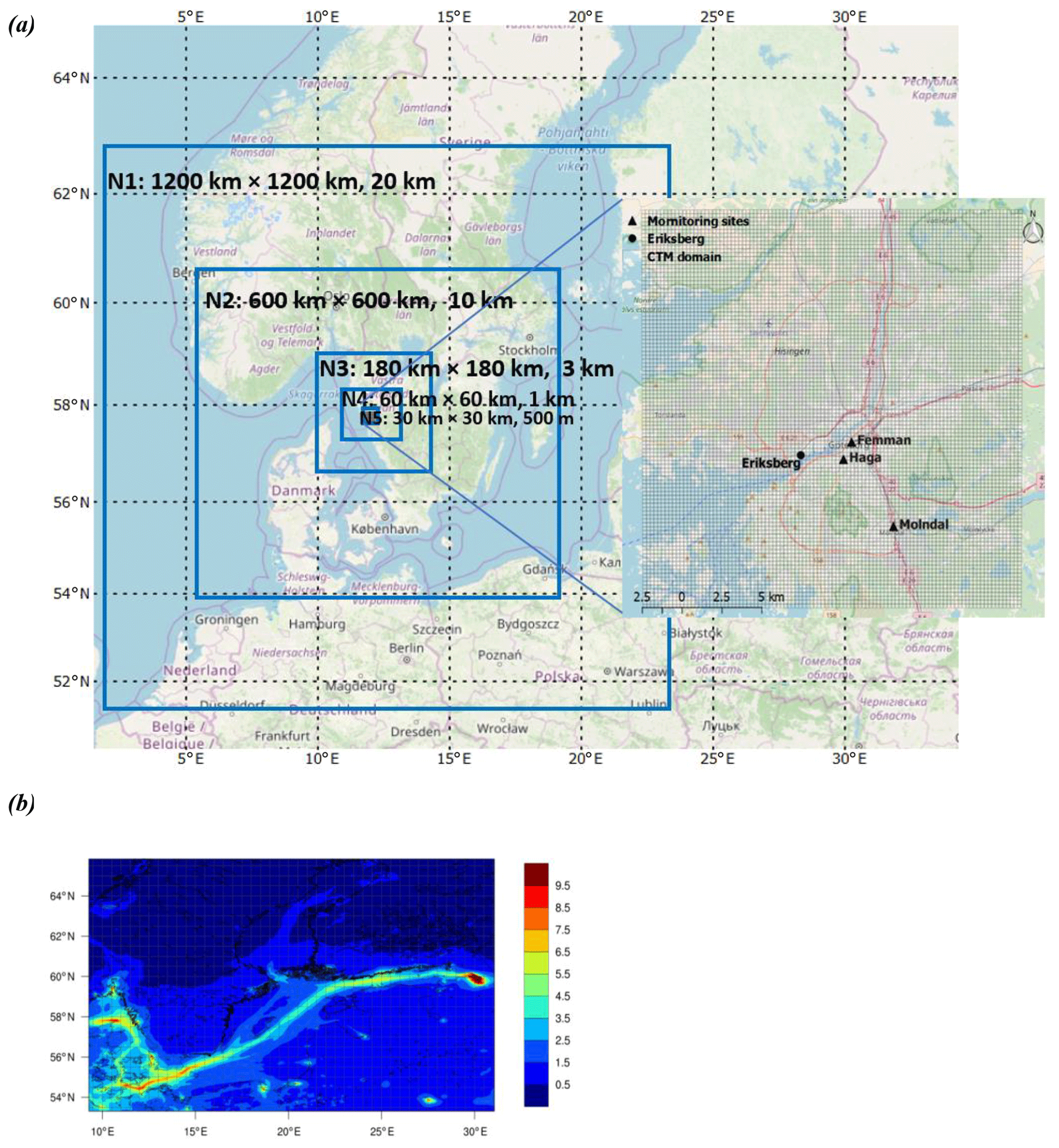
Figure 1(a) Five nested meteorological model domains with their sizes and spatial resolutions. The fifth domain with an air pollution grid (250 m×250 m) is pointed out in the figure, showing the location of the three air quality monitoring sites Femman, Haga and Mölndal as well as Eriksberg, a residential area close to the harbour. (b) The boundary conditions of air pollution in TAPM; example of summer mean (JJA) 2012 NO2 concentrations (ppbV) in the regional-scale CMAQ simulation (4 km×4 km). Base map credits: © OpenStreetMap contributors 2020. Distributed under a Creative Commons BY-SA License.
The chemical boundary conditions were taken from the Community Multiscale Air Quality Modeling System (CMAQ; Byun and Ching, 1999; Byun and Schere, 2006). CMAQ model simulations on a 4 km ×4 km grid (Karl et al., 2019c), which were used for the chemical boundary conditions (Fig. 1b), were driven by the high-resolution meteorological fields of the Consortium for Small-scale Modelling (COSMO) Climate Limited-area Modelling Community (CLM; Rockel et al., 2008) version 5.0 using the ERA-Interim reanalysis as forcing data. Chemical boundary conditions for the CMAQ model simulations were provided through hemispheric CTM simulations from a System for Integrated Modelling of Atmospheric Composition (SILAM) model (Sofiev et al., 2006) run on a grid resolution, which was provided by the Finnish Meteorological Institute (FMI). Land-based emissions for the regional-scale simulations were represented by hourly gridded emissions calculated with the SMOKE-EU (Sparse Matrix Operator Kerner Emissions, EU version) emission model (Bieser et al., 2011). The SMOKE-EU emission data are based on reported annual total emissions from the European Pollutant Emission Register (EPER), the official EMEP emission inventory (https://www.ceip.at/, last access: 11 June 2020) and the EDGAR HTAP (Emission Database for Global Atmospheric Research, project of the Hemispheric Transport of Air Pollution task force) v2 database (EPER, 2018; CEIP, 2018; Olivier et al., 1999). For shipping emissions, the model used an inventory calculated with the Ship Traffic Emission Assessment Model (STEAM) consistent with the inventory used by TAPM for the city-scale, calculated with 2 km ×2 km grid resolution (STEAM3, Johansson et al., 2017); more details are given in the next section. The STEAM version used for the CMAQ simulations did not, however, include VOC emissions. As chemical boundary conditions, vertical model layer 7 with a mid-layer height of approximately 385 m above ground was selected. CMAQ simulations with and without ship emissions in the Baltic Sea and the North Sea included were used in TAPM simulation runs. Since TAPM allows just 1-D boundary concentration fields with hourly time resolution, TAPM boundary concentrations were calculated using the horizontal wind components on each of the four lateral boundaries for weighting the upwind boundary concentrations around the domain of TAPM (Fridell et al., 2014). The city-scale model set-up is summarized in Table 1.
2.2 Emission inventory
2.2.1 Regional and local shipping emissions
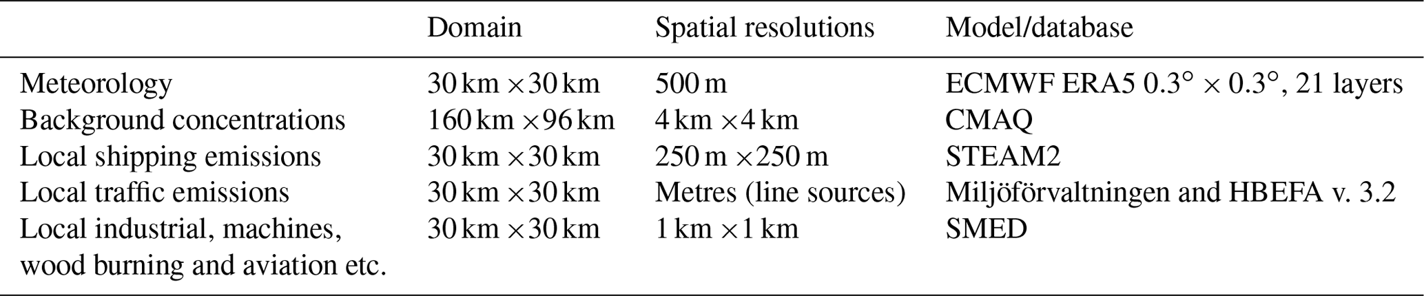
Shipping emissions were calculated with STEAM, taking into account individual vessel characteristics and vessel activity data (Jalkanen et al., 2009, 2012 Johansson et al., 2017) based on detailed information of technical parameters of individual vessels and position data of individual ships taken from reports from the Automatic Identification System (AIS) of the Helsinki Convention (HELCOM) member states. STEAM calculated fuel consumption and emissions as functions of vessel activity; the STEAM3 version of the model has been used (Johansson et al., 2017) with an additional module for the calculation of VOC emissions. The emission inventory includes combustion emissions from all engines and appliances on ships (boilers, auxiliary and main engines). The emission inventory for local shipping around Gothenburg consists of hourly emissions from ships on 250 m ×250 m grid resolution. STEAM provided shipping emissions for the year 2012 for the compounds NOx, SOx, CO, CO2, VOC and PM2.5. PM2.5 is further divided into elemental carbon (EC), organic carbon (OC), and mineral ash. Ship emissions were provided in two vertical layers with emissions below and above 36 m height in order to differentiate between emissions from large ships with high stacks and the smaller vessels with lower stack heights (Fig. 2). The stack release heights were attributed to the corresponding midpoints of model layers in TAPM: 15 m for the emissions below 36 m height and 36 m for emissions above 36 m.
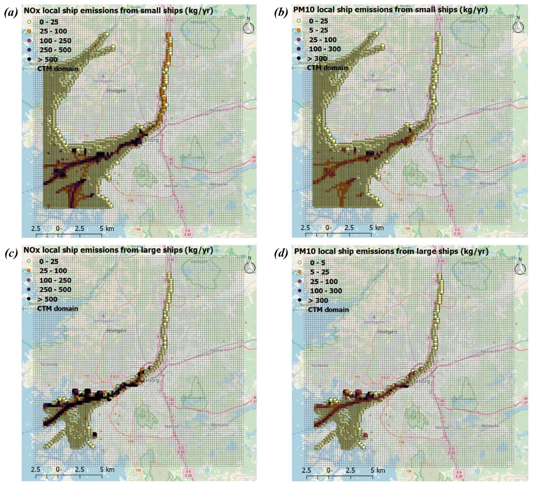
Figure 2Annual local shipping emissions of (a) NOx and (b) PM10 (equal to PM2.5) from small vessels with a stack height below 36 m (assumed 15 m) and (c) NOx and (d) PM10 from large vessels with high stack height above 36 m (assumed 36 m) in the Gothenburg area. Base map credits: © OpenStreetMap contributors 2020. Distributed under a Creative Commons BY-SA License.
2.2.2 Road traffic emissions
The road traffic emissions were calculated from traffic activity data and emission factors. The basic set of emission factors from road vehicles was extracted from the HBEFA v. 3.2 (Handbook Emission Factors for Road Transport; Rexeis et al., 2013). The HBEFA comprehends emission factors for different classes of road vehicles based on type of vehicle (e.g. motorcycles, light-duty vehicles, heavy-duty vehicles), technology or fuel (e.g. petrol, diesel, hybrid) and emission standard (pre-Euro, Euro 6). For each of those, a number of road categories and driving patterns that affect emissions are also specified within the vehicle sub-segments. These emission factors also include emissions of wear particles as well as evaporative VOC emissions. The emission factors for light-duty and heavy-duty vehicles and busses in Gothenburg were calculated using the Swedish national database on car fleet composition and national vehicle-type-specific activity data in 2012. Road traffic emissions were finally calculated using traffic activity data for Gothenburg (vehicle kilometres for light-duty vehicles plus motorcycles, heavy-duty vehicles and busses on road links with specified type, speed and congestion hours) from the database of the Environmental Administration, City of Gothenburg (Miljöförvaltningen), and corresponding emission factors calculated in the HBEFA database. These data were applied as line emission sources in the model. Resuspension of the road dust is not covered in the model.
2.2.3 Other emissions
Ten large point sources from industrial processes are present in the city-scale model domain; these are all fugitive emissions from fuel handling and refineries. For technical reasons these were considered as area sources in the model with release heights corresponding to the stack heights allocated to these sources. The emission factors from these industrial sources were obtained from Swedish Environmental Emissions Data (SMED, 2015) for 2012.
Emissions from the following sectors were geographically distributed on a 1 km ×1 km grid and assigned an emission height: “manufacture of solid fuels and other energy industries”, “combustion in industry for energy purposes”, “stationary combustion in agriculture/forestry/fisheries”, “energy and heat production (commercial/institutional)”, “residential plants (boilers), domestic heating, working and off-road machinery”, “use of paints and chemical products in households and enterprises”, “agriculture, waste and sewage” or “other transports” (the landing and take-off emissions from aviation, trains and military). They also stem from the SMED database and were obtained gridded on the 1 km ×1 km grid from the SMHI (Swedish Meteorological and Hydrological Institute). These emissions were applied as gridded sources in the model.
The local emissions of NOx, SO2, PM10 and VOCs from the above-mentioned sectors in the model domain are shown in Fig. 3. Local shipping was the dominant emission source of SO2, contributing 61 % of the total SO2 emissions (502 t yr−1) in the model domain. Further, local shipping contributed 41 % of NOx emissions in the model domain, which was comparable to the contribution from road traffic (47 %) to total NOx emissions of 5072 t yr−1. However, road traffic was the most major contributor of PM10 in the model domain (45 % of 357 t yr−1), while local shipping and industry contributed approximately 25% each. For VOCs (7457 t yr−1), about 92 % of emissions were released from the industrial sector and only 0.3 % from local shipping.
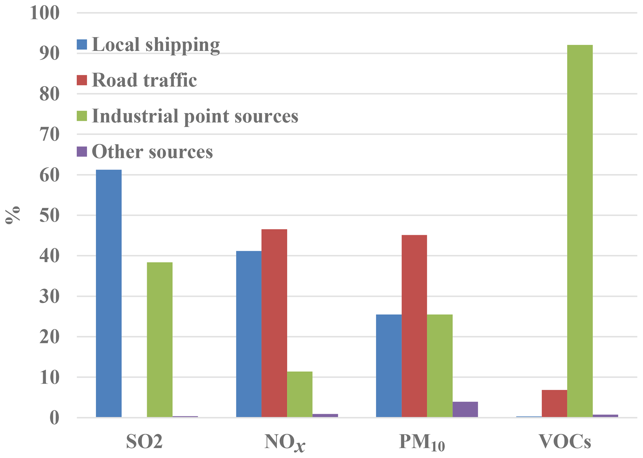
Figure 3Proportions of different source categories in the local emission inventory for the city-scale model domain in the year 2012. The total emissions are 502 t yr−1 for SO2, 5072 t yr−1 for NOx, 357 t yr−1 for PM10 and 7457 t yr−1 for VOCs.
2.3 Design of model simulations
Several model simulations were performed to investigate the influence of shipping within the city domain and influence of regional shipping outside the city on air pollution in 2012:
-
a simulation including complete emission inventory both in the city-scale simulation and in the CMAQ simulation supplying the chemical boundary conditions (“base scenario”)
-
a simulation excluding local shipping in the city domain of TAPM but including regional shipping chemical boundary conditions in the CMAQ simulation (“no local shipping scenario”)
-
a simulation excluding both local shipping in the city domain of TAPM and shipping in the chemical boundary conditions in the CMAQ simulation (“no local and regional shipping scenario”).
In addition, three sensitivity studies were performed within this study:
-
“No NMVOC from local shipping” had the same emission input as the “base scenario” but without NMVOC from local shipping emissions. The difference between “base” and “no NMVOC from local shipping” was used to investigate the impact of VOC emissions from local shipping, which is often neglected in the emission inventories due to its small proportion and as these have only recently been included in STEAM.
-
“Primary PM from local shipping” had the same emission input as the “base scenario”, but for local shipping only the primary PM emissions as calculated by STEAM were included. All emissions of the gaseous species were excluded, preventing the formation of the secondary PM from local shipping. The difference between “base scenario” and “primary PM from local shipping” reflects the formation of the secondary PM from SO2, NOx and VOC emitted by local shipping.
-
“No road traffic” had the same emissions as the “base scenario” but without road traffic emissions. It was used to compare the contributions of shipping emissions as well as the health impact of shipping with emissions from city traffic.
2.4 Model evaluation
Model evaluations were carried out for both meteorological and air pollution parameters. The simulated meteorological parameters (temperature, relative humidity, wind fields and precipitation) were evaluated with measurements at four stations: Femman (57.70∘ N, 11.97∘ E; 30 m a.s.l.), Göteborg A (57.72∘ N, 11.99∘ E; 3 m a.s.l.), Vinga A (57.63∘ N, 11.60∘ E; 18 m a.s.l.) and Landvetter (57.68∘ N, 12.29∘ E; 154 m a.s.l.). The urban background site Femman is located on a rooftop in the city centre, and the local meteorological variables as well as the air quality data are continuously measured by the Environmental Administration in Gothenburg (Miljöförvaltningen), while the other three meteorological stations are driven by the SMHI. For the air pollution evaluation, Femman, Haga and Mölndal were included. Haga is located in a one-sided street canyon in central Gothenburg with a park to the east of the station. Mölndal is located in southern part of Gothenburg on a rooftop about 30 m above ground and corresponds to a traffic station. NO2 is measured via a reference chemiluminescent method at Femman and Haga and the differential optical absorption spectrometry (DOAS) method at Mölndal. PM10 mass concentrations are measured by a TEOM (tapered element oscillating microbalance; Thermo Fisher Scientific, model 1400ab) instrument at all three stations. The ozone instrument at Femman was Teledyne (model T400) and at Mölndal a DOAS from OPSIS. Hourly averaged air quality data for NO2, PM10, PM2.5 and O3 at the three air quality stations were used to evaluate the model performance.
The FAIRMODE DELTA tool version 5.4 was used for the evaluation of the model results for the city of Gothenburg. The DELTA tool is an IDL (interface definition language)-based statistical evaluation software which allows for the performance diagnostics of the air quality and meteorological model (Thunis et al., 2012; Pernigotti et al., 2020). The tool focuses on the air pollutants regulated in the Air Quality Directive 2008 (AQD 2008) and calculates statistical performance indicators such as mean, exceedance, normalized mean bias (NMB), normalized mean standard deviation (NMSD) and high percentile (Hperc; see Sect. S1 in the Supplement). Moreover, a performance criterion can be calculated that combines the statistical performance indicators with fixed parameters to evaluate whether the model results have reached a sufficient level of quality for a given policy support application (Pernigotti et al., 2020). According to the DELTA tool, the capability of a model to reproduce measured concentrations is good when more than 90 % of the stations fulfil the performance criterion. We applied the DELTA tool to concentrations of NO2, PM2.5, PM10 and O3 measured at the available urban background sites and road traffic sites, compared them with concentrations calculated by our model system and calculated both statistical performance indicators and the model performance criterion.
2.5 Health impact assessment
The health impacts of exposure of the population in Gothenburg to shipping-related air pollutants were assessed with the ALPHA-RiskPoll (ARP) methodology (Holland et al., 2013), which provides for the calculation of a wide range of air-pollutant-specific health effects based on the population-weighted concentrations, national population statistics on age distribution of the population, mortality and morbidity data and effect-specific exposure–response relationships. The methodology has been developed and used for the quantification and assessment of the benefits of air pollution controls in Europe for the United Nations Economic Commission for Europe (UNECE) Convention on Long-Range Transboundary Air Pollution and is based on work for the Clean Air For Europe (CAFE) programme and on the EU project Modelling of Air Pollution and Climate Strategies (EC4MACS). Following WHO recommendations (WHO, 2013a) and the CAFE cost–benefit analysis methodology for the assessment of health impacts of air pollutants; the impacts have been considered following WHO recommendations and CAFE. Exposure to these three pollutants is considered most harmful by the World Health Organization (WHO, 2013b). In this study only the most serious impacts (i.e. loss of life) are presented, taking into account the impacts of long-term exposure to PM2.5 and short-term exposure to ozone and NO2, i.e. the impacts marked A* in the HRAPIE study (WHO, 2013a). The indicator SOMO35 is used for ozone, representing the yearly sum of the daily maximum of the 8-hour running average above a threshold of 35 ppb. The health impacts of some pollutants are correlated, and that is why the premature deaths attributed to each pollutant cannot simply be added up. In particular, it has been estimated that adding premature deaths attributed to PM2.5 to those attributed to NO2 could result in double-counting of around 30 % (WHO, 2013a). The health impacts calculated with the ARP model are presented as premature deaths and YOLLs per year using the ER function of the model, i.e. 1.0062 (95 % confidence interval is 1.004–1.008) per µg m−3 (WHO, 2013a).
The concentration fields of PM2.5, O3 and NO2 were calculated by the coupled high-resolution (250 m ×250 m) modelling system as described above. Annual means and SOMO35 were calculated from hourly concentrations for each grid. Population data at 1 km ×1 km resolution were obtained from Statistics Sweden (SCB) for 2015, with a population of 572 779 in the city of Gothenburg. As there were no significant changes in population density between 2012 and 2015, the population data for 2015 were used. Population-weighted average concentrations (PWCs) for the model domain were calculated by multiplying the modelled annual mean concentration of the pollutant on each grid cell by the population in the same grid cell as weight for the modelled concentration.
To calculate the health risks, the ERF and the baseline health statistics including the life expectancies, the death rates and morbidity data for estimating the impacts on mortality and morbidity are also needed. To estimate YOLLs, the age at which the premature deaths occurred should also be considered. In the ARP model, the ERFs used are those from the WHO (2013a): 6.2 % (95 % confidence interval is 4.0 %–8.3 %) relative risk increase per 10 µg m−3 of increased exposure for the PM2.5 exposure, 0.29 % (95 % confidence interval is 0.14 %–0.43 %) relative risk increase per 10 µg m−3 of increased exposure for the ozone exposure and 0.27 % (95 % confidence interval 0.16 %–0.38 %) relative risk increase per 10 µg m−3 of increased exposure for the NO2 exposure. The ARP uses linear ERFs, recognizing the limited range of pollutant exposures in Europe. The YOLLs are calculated per year, applying the relative risk within national life tables. This is done through relation between the years of life lost per 100 000 people per unit PM2.5 concentration and the life expectancy of the population developed by Miller et al. (2003) based on analysis of the life tables. The premature deaths are calculated using the ERF for all-cause mortality and the total national mortality rates. This methodology is justified for European countries with a health status and proportion of natural mortality of the population corresponding to the population studied in the epidemiological studies which brought forward these ERFs. For regions with high concentration levels of PM2.5 the HIA studies need to use different forms of ERFs, and for populations with a different health status and proportion of natural mortality compared to the US and Western Europe, cause-specific rather than all-cause mortalities need to be used. In this study the analysis was made separately for the population exposure related to the different pollutants from local and regional shipping.
3.1 Model evaluation
The model evaluation was conducted for both meteorology and air pollution in the innermost model domain. The comparison between hourly measured and modelled local meteorological parameters (temperature, relative humidity, total solar radiation, wind speed, wind direction and precipitation) shows a high correlation and low bias: averaged over all available stations, temperature and wind speed are slightly underestimated at −0.46 ∘C and −0.18 m s−1, respectively. A detailed analysis can be found in Table S1 in the Supplement. The application of ERA5 datasets in the model shows significant improvements from the default reanalysis datasets. Nevertheless, the predictions of the meteorological parameters such as wind field flow get better with wind field assimilation; for more detail see Ramacher (2018). For example, the differences between observed and simulated wind rose at Femman in January and July, indicating the model's good capability of reproducing local wind field except for the missing ∼30 % of low wind speeds (0–2.5 m s−1) from the north (Fig. 4), which may introduce some underestimations in high pollutant concentrations at the ground due to accumulation in the boundary layer. Nevertheless, the total frequency of northerly winds at Femman station is low in January (8 %–17 %) and very low in July (1 %–8 %).
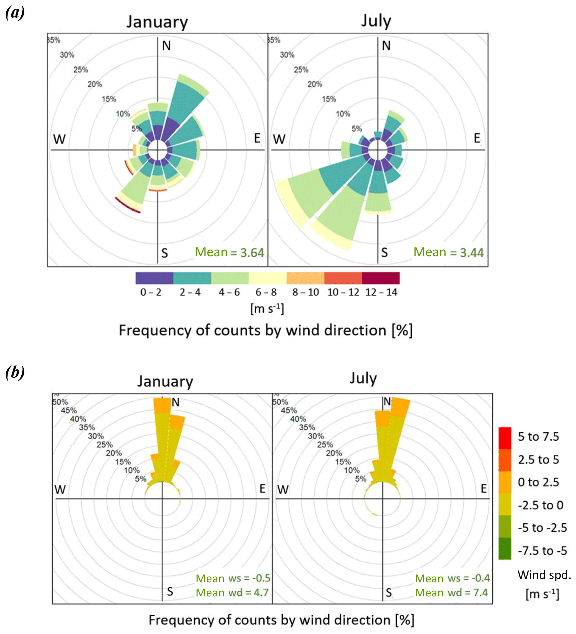
Figure 4Comparison between measured and modelled winds at Femman station: (a) the observed wind rose in January and July and (b) bias of the wind speed based on the difference between simulated wind speed and measured wind speed. For example, a positive bias from 0 to 2.5 m s−1 in wind direction N has a frequency of almost 30 %.
The evaluation of ambient pollutants was conducted through the major statistical parameters (Table S2). At the urban background site Femman, the estimation of NO2, PM10 and PM2.5 concentrations was satisfactory in summer, with a lower bias (−0.16 µg m−3); however the model tended to underestimate NO2, PM10 and PM2.5 concentrations in winter (−15.35 µg m−3). O3 evaluation was carried out at Femman and Möldal stations, and underestimation of the daily maximum of the 8 h means was also detected, which could be caused by the low resolution of local NO sources and hence more smoothed titration of ozone. The summary statistics according to the FAIRMODE model evaluation tool shows that less than 90 % of daily PM10 concentrations at the road site Haga fulfil the performance criteria for the statistic indicator Hperc (Fig. 5). The indicator Hperc indicates the model's capability of reproducing extreme events, represented by a selected high percentile for modelled and observed values. A detailed evaluation of simulated concentrations in the form of scatter plots of modelled versus measured daily concentrations can be found in Fig. S1 in the Supplement.

Figure 5Summary statistics of model performance for the annual mean values of (a) NO2 (hourly values), (b) PM10 (daily values), (c) PM2.5 (daily values) and (d) O3 (daily maximum of the 8 h means), including days of exceedances. Stations (blue dots) within the green bars: performance criteria satisfied; stations within the orange bars: performance criteria satisfied, error dominated by the corresponding indicator. Green light: > 90 % of the stations fulfil the performance criteria. Red light: < 90 % of the stations fulfil the performance criteria. The indicator Hperc indicates the model's capability of reproducing extreme events, represented by a selected high percentile for modelled and observed values.
The underestimation of NO2 and PM10 especially at road sites demonstrates the impact of too coarse spatial resolution (250 m ×250 m) not capturing high concentrations at the street level, possible missing or insufficient cover of local emissions like resuspension particulate matters from traffic sources, and incomplete chemical reactions in the model etc. As pointed out by Karl (2018), recent nested model approaches have not resolved the details in emission processing and near-field dispersion at the street and neighborhood level. However, shipping emissions are, when reaching the exposed population, more dispersed, and the 250 m×250 m grid resolution should be sufficient to assess their impact. Nevertheless, the other statistic indicators (mean, exceedances, normalized mean bias, normalized mean standard deviation, correlation coefficient, etc.) of model performance in Fig. 5 show a satisfactory performance of the used city-scale model for Gothenburg.
3.2 Impact of ship emissions on local air quality
3.2.1 SO2
The study was performed for 2012 conditions, when the sulfur content in marine fuels was limited to 1 % in the region and 0.1 % for ships at berth. With these fuel sulphur limits, local shipping is still the dominant local emission source of SO2 (60 %) and influences the area around main shipping routes and city ports (Fig. 6). The calculated annual mean concentration of SO2 from all sources in the model domain is 0.4 ppb, and local shipping contributes 0.05 ppb (13 %) to the model domain average and between 0.3 ppb and up to 0.6 ppb in a wide area around the main shipping routes and ports. The impacts were higher in summer than in winter (Fig. S2) as a result of higher shipping emission in summer as well as of differences in the meteorological situation. The highest SO2 contributions (maximum of 0.7 ppb to the annual mean and 0.8 ppb in summer) were found around the major ports (Älvsborgshamnen, Skandiahamnen, Skarvikshamnen, Ryahamnen, Lindholmshamnen and Frihamnen) along the northern bank of the Göta älv (Fig. 6d). In addition, two busy ferry terminals located on the southern bank of the Göta älv can contribute to the high SO2 concentrations on the opposite side of the river due to the dominant south-westerly winds. The regional ship emissions outside the model domain contribute an additional 0.06 ppb (15 %) to the model domain average. In contrast to local shipping, this contribution is distributed rather evenly over the model domain.
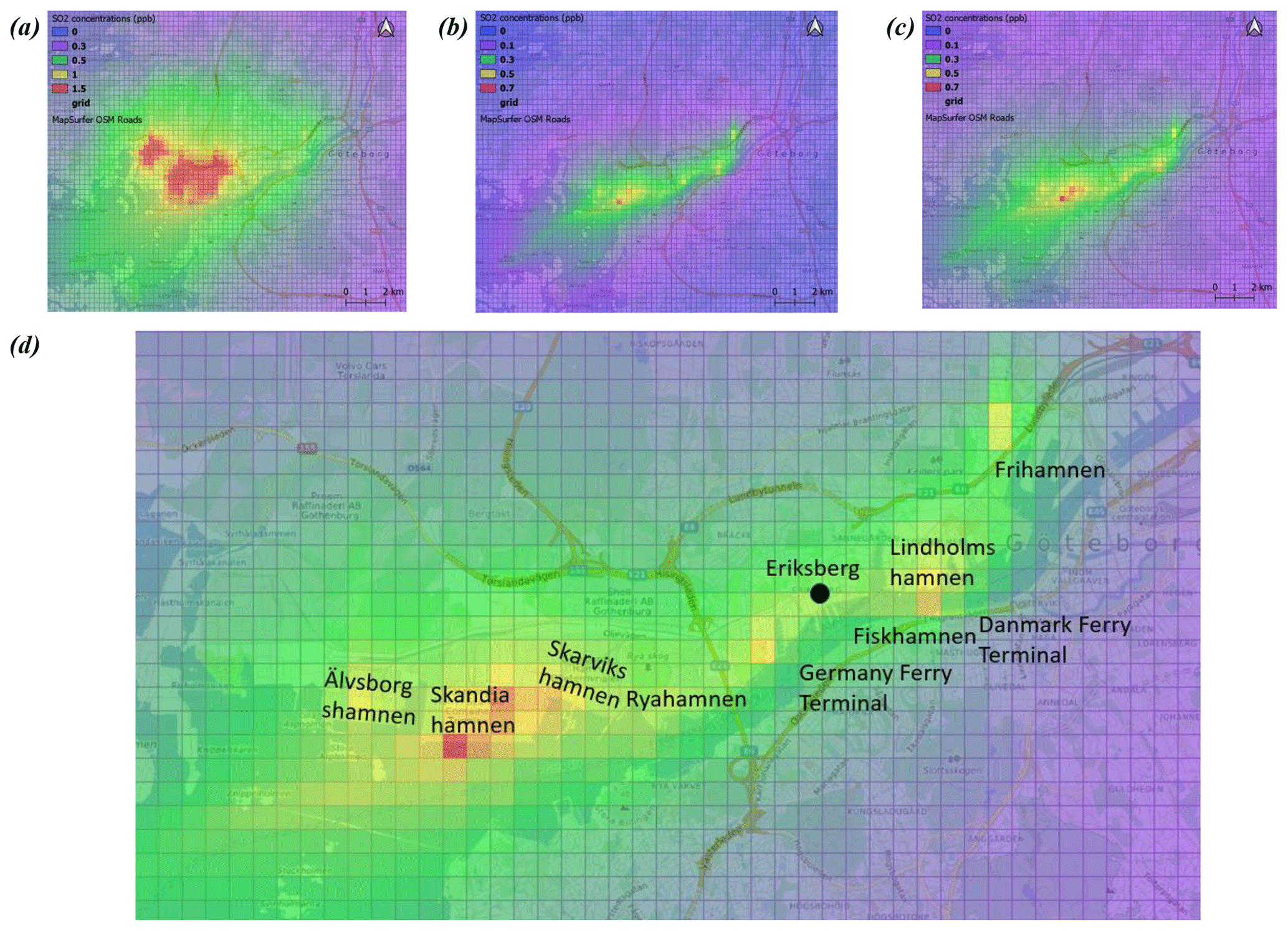
Figure 6Simulated atmospheric concentrations of SO2 (in ppb) for the year 2012: (a) annual mean concentrations in the base case simulation, (b) annual mean contribution of local shipping, (c) annual mean contribution of local and regional shipping and (d) same as (c) but with main ports along the Göta älv as well as Eriksberg. Base map credits: © OpenStreetMap contributors 2020. Distributed under a Creative Commons BY-SA License.
The modelled SO2 concentrations in Gothenburg are relatively low, and Fig. 6 shows the highest concentrations around the city ports as well as around industrial areas north of the Göta älv. The dominated south-westerly winds transport emissions from the shipping routes and port areas further inland to the north. Today, Eriksberg, located on the north waterfront of Göta älv, is a modern residential and commercial centre built at the site of a former dockyard area. We have selected this place to study the relative impact of shipping in more detail. The shipping-related monthly contributions to SO2 concentrations at Eriksberg were 47 % on average and over 60 % between June and August. Figure S3 shows the modelled monthly mean relative contributions at Eriksberg.
3.2.2 NO2
NOx is mainly emitted as nitrogen oxide (NO); in STEAM the NO2∕NOx ratio is 5 %. In the atmosphere NO is quickly converted to NO2 in reaction with ozone, so further from the source the atmospheric NOx is dominated by NO2, approaching a photostationary state driven by the NO+O3 reaction and NO2 photolysis. Maps of modelled annual mean atmospheric concentrations of NO2 over the Gothenburg area are shown in Fig. 7. The annual mean concentration of NO2 in the base simulation is 3.7 ppb as the model domain average (Fig. 7a), and the model domain mean contribution from local shipping to the annual mean concentrations is 0.5 ppb (14%) and up to 3.3 ppb in areas with a high contribution (Fig. 7b). The relative contribution of local shipping to the NO2 concentrations in the model domain in Gothenburg is comparable with 11 % in Riga (Latvia), 16 % in Gdańsk–Gdynia (Poland) and 22 % in Rostock (Germany) in 2012 (Ramacher et al., 2019). The calculated model domain mean contribution to NO2 concentrations from regional shipping is 1.0 ppb (26 %) and up to 1.2 ppb in the most heavily impacted areas (Fig. 7c), which is larger than local shipping contributions. The total shipping-related relative contribution in Gothenburg to the NO2 annual mean in the model domain is 40 %. In summer the contribution reaches 49 % (17 % from local shipping + 32 % from regional shipping) to the average summer NO2 concentration in the model domain, and influenced areas expand further inland. This is the result of 20 % higher summer emissions compared to winter, a different photochemical state and different local meteorological conditions (Fig. S4).
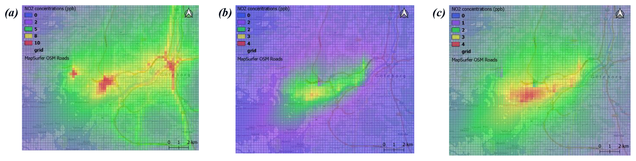
Figure 7Simulated atmospheric concentrations of NO2 (in ppb) for the year 2012: (a) annual mean concentrations in the base case simulation, (b) annual mean contribution of local shipping and (c) annual mean contribution of local and regional shipping. Base map credits: © OpenStreetMap contributors 2020. Distributed under a Creative Commons BY-SA License.
Nearly 90 % of NOx emissions in Gothenburg are from road traffic (47 %) and local shipping (41 %). The impact of local shipping is concentrated in areas inside the harbour along the Göta älv and decreases with growing distance to the port areas. Figure 8 presents the impacts of local and regional shipping as well as of road traffic and all other anthropogenic sources (including NO2 coming from the model domain boundary) on monthly levels at Eriksberg. The modelled annual mean NO2 concentration from all sources is 7.5 ppb at Eriksberg, of which 2.5 ppb (33 %) originates from local shipping, 1.0 ppb (13 %) from regional shipping and 2.1 ppb (28 %) from road traffic. The maximum relative contributions from local shipping and regional shipping to the monthly mean concentrations reach 43 % in July and 16 % in June. Together, the monthly average contributions from local and regional shipping are larger than or comparable to the contributions from road traffic in all months. Even though road traffic is a major contributor to the NO2 concentrations in an urban environment, local ship emissions are of major concern, especially in areas close to the city ports.

Figure 8Modelled monthly mean contribution of the local shipping, regional shipping, local road traffic and other anthropogenic emissions (including the contribution from the boundary conditions) to the NO2 concentrations at Eriksberg in the year 2012.
3.2.3 O3
O3 is formed in photocatalytic cycles involving NOx, ozone and hydrocarbons through the photolysis of NO2 in sunlight. The same cycle also involves the titration of ozone by the reaction with NO forming the NO2. Maps of modelled atmospheric concentrations of ozone over the Gothenburg area in 2012 are shown in Fig. 9, with a focus on summer months (JJA). The regional background concentration of ozone at the regional background station Råö, close to the Gothenburg area, was 37 ppb in the summer of 2012. Modelled summer ozone levels in the model domain are in the 15–30 ppb range (domain average is 28.6 ppb; Fig. 9a). Since NOx is mainly emitted as NO, the emissions from local shipping cause local reduction of ozone concentrations by 0.5 ppb (∼2 %) in the main shipping routes and port areas due to the titration of O3 by NO (Fig. 9b). The maximum O3 depletion along the north riverbank of the Göta älv is 4 ppb (∼14 %) with both NOx and non-methane volatile organic compound (NMVOC) emissions from local shipping (Fig. 9b), while regional shipping emissions increase the ozone concentrations by 1 ppb over the land. This ozone increase can be compared to the 4–6 ppb increase caused by shipping emissions over the remote ocean as a result of large-scale summer ozone production found by Huszar et al. (2010, Fig. 9c).
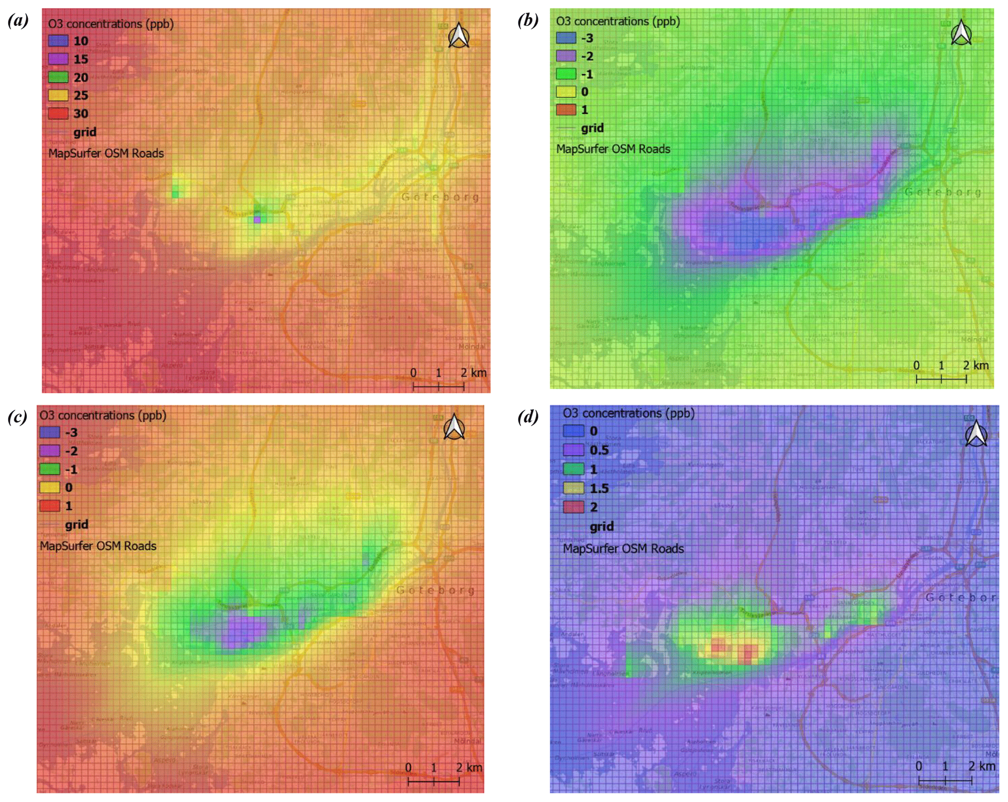
Figure 9Modelled summer mean (JJA) ozone concentrations (ppb) in the year 2012 and contributions of local and regional shipping: (a) modelled O3 concentrations in the Base model simulation, (b) modelled contribution of emissions from local shipping, (c) modelled contribution of emissions from local and regional shipping and (d) modelled contributions of NMVOC emissions from local shipping. Base map credits: © OpenStreetMap contributors 2020. Distributed under a Creative Commons BY-SA License.
In the local STEAM inventory, the NMVOCs from shipping were introduced. These NMVOCs serve as precursors of O3 and enhance photochemical ozone production. TAPM uses the concept of VOC reactivity instead of individual NMVOCs, producing a pool of peroxy radicals which take part in the ozone production photocatalytic cycle. A sensitivity run was performed to study the impact of VOC emissions from local shipping on ozone concentrations in the city by excluding the local shipping VOC emissions from the simulation. Figure 9d shows the impact of the VOC emissions: the O3 concentrations increase by up to 2 ppb (∼7 %) along the main shipping routes and the port areas, which means that the titration effects of NOx emissions from local shipping on the ozone concentrations were maximally 6 ppb when VOC emissions were excluded, compared to 4 ppb in the Base simulation. Sensitivity of ozone formation to VOC emissions also clearly indicates that the city centre is most often in a VOC-limited regime. Further details of the impact of shipping emissions on ozone formation are illustrated in Fig. S5, showing summer ozone formation from regional and local shipping as well as from local shipping VOC emissions at Eriksberg. At this location local shipping emissions almost always lead to ozone depletion. In contrast, VOC emissions from local shipping cause the increase in ozone concentrations, confirming that the location is in a VOC-limited photochemical regime. Regional shipping tends to increase local ozone concentrations on most days (78 d between June and August). Inspecting the details of the diurnal variation of ozone contributions (Fig. S5b–d), one can see that during the rare occasions without ozone depletion by local shipping, there is a small amount of ozone formation from local shipping emissions and no ozone formation from local shipping VOC emissions, indicating the presence of a NOx-limited regime (Fig. S5b), whereas during most of the studied days local shipping emissions have an ozone depletion effect during daytime, while the ozone formation effect of local shipping VOC emissions peaks in the morning and sometimes also in the afternoon (Fig. S5c). Regional shipping increases the ozone concentrations in all three depicted cases, showing maxima in the afternoon.
3.2.4 Particulate matter
Particulate matter includes primary, directly emitted particles and secondary particulate matter formed upon further processing of emissions in the atmosphere. At the urban background site Femman, close to the city harbour, the measured annual mean PM2.5 concentration was 7.9 µg m−3 in 2012. The calculated annual mean PM2.5 in the base simulation is 4 µg m−3 as the model domain average (Fig. 10a). Local shipping emissions contributed 0.1 µg m−3 (3 %) of the annual mean as the model domain average (Fig. 10b), which had the same relative contribution as 3 % in Gdańsk–Gdynia and higher than 1 % in Rostock and Riga in 2012 (Ramacher et al., 2019). Under 2012 conditions, regional shipping was a larger contributor to the local PM2.5 than local shipping, with an annual mean average contribution of 0.4 µg m−3 (11 %; Fig. 10c). The total shipping-related relative contribution to the annual averaged PM2.5 concentrations in the model domain was 14 % and in the summer reached 27 % (4 % from local shipping +23 % from regional shipping) of the summer averaged PM2.5 concentrations in the model domain (Fig. S6). At the near-harbour residential area Eriksberg the modelled annual mean PM2.5 concentration from all sources is 4.5 µg m−3. The calculated annual mean contributions from local shipping and regional shipping are 0.2 µg m−3 (∼4 %) and 0.4 µg m−3 (∼9 %), respectively. The maximum monthly relative contribution from local and regional shipping was about 29 % in July, of which 21% was from regional shipping (Fig. 11). Road traffic, the largest local source of PM10, contributed up to 5% of monthly PM2.5 mean concentrations. The large contribution of PM2.5 from regional shipping is in agreement with the character of source apportionment in Gothenburg. An early study shows that the main source types of PM2.5 in Gothenburg were long-range transport (LRT; about 50 %) followed by ship emissions (20 %) and local combustion (19 %) between 2008 and 2009 (Molnár et al., 2017).
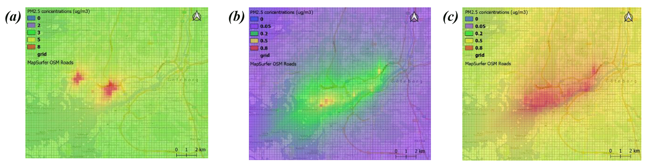
Figure 10Modelled annual mean PM2.5 concentrations (µg m−3) and contributions of shipping in the year 2012: (a) modelled annual mean concentrations in the base model simulation, (b) modelled annual mean contribution of local shipping and (c) modelled annual mean contributions of local and regional shipping. Base map credits: © OpenStreetMap contributors 2020. Distributed under a Creative Commons BY-SA License.
The secondary aerosol formation in TAPM is heavily parameterized; however, it captures the important features of the secondary particle formation, i.e. formation of sulphate and nitrate following SO2 and NO2 oxidation as well as formation of SOA as a fixed part of the degraded smog reactivity representing VOC species in the reaction scheme of TAPM (Hurley, 2008b). On an urban scale, formation of secondary PM is usually suppressed as the radical pool is depleted by the primary emissions, and many urban models do not consider the secondary PM at all. Therefore, a sensitivity run was performed to investigate the role of the formation of secondary PM from local shipping on the city scale, where only emissions of the primary PM were introduced, without emissions of the gas-phase pollutants from local shipping. Modelled secondary PM concentrations from shipping were calculated as the difference between the base run and this sensitivity run. Figure S7 shows contributions of max. 2 % of the PM related to local shipping in Gothenburg in the winter months and negligible contributions in summer. The secondary PM, mainly formed far from the sources, tends to disperse and accumulate in the eastern part of Gothenburg due to the prevailing wind directions.
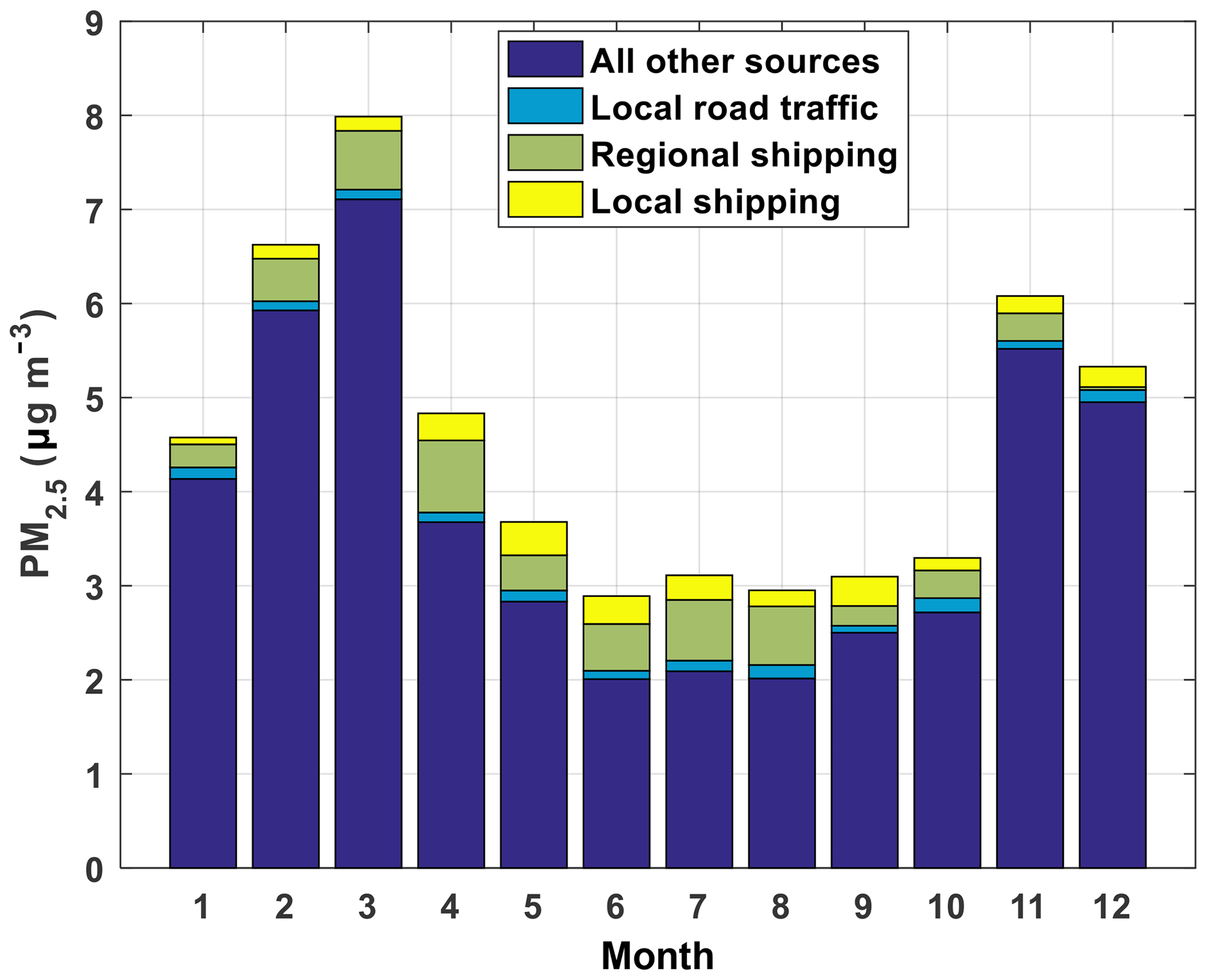
Figure 11Modelled monthly mean contributions from local shipping, regional shipping and other sources (including contribution from the boundary condition) to PM2.5 concentrations at Eriksberg for the year 2012.
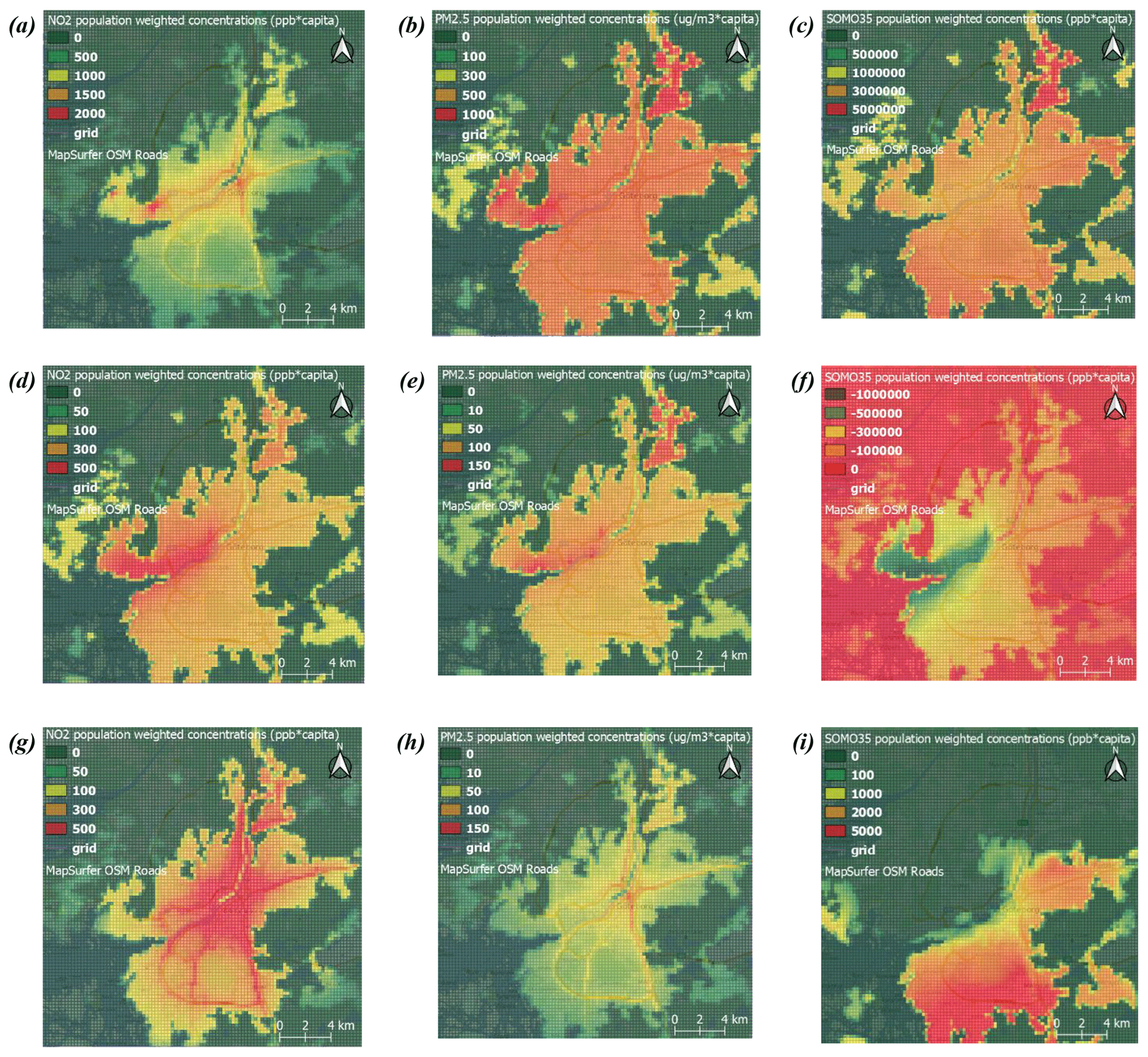
Figure 12The population-weighted annual mean concentrations for NO2 (ppb × capita), PM2.5 (µg m−3 × capita) and SOMO35 (ppb × h × capita): (a) NO2 in the base simulation, (b) PM2.5 in the base simulation, (c) SOMO35 in the base simulation, (d) NO2 from local and regional shipping, (e) PM2.5 from local and regional shipping, (f) SOMO35 from local and regional shipping, (g) NO2 from road traffic, (h) PM2.5 from road traffic and (i) SOMO35 from road traffic. Base map credits: © OpenStreetMap contributors 2020. Distributed under a Creative Commons BY-SA License.
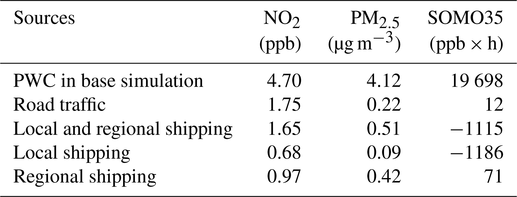
The contribution of emission sources to population exposure depends on the relationship between population density and air pollution levels. The areas with relatively high exposure to PM2.5 due to local and regional shipping are city ports and areas around and especially north of the Göta älv. Figure 12 presents the population-weighted annual mean concentrations of NO2, PM2.5 and SOMO35 at each model grid for the base simulation and for contributions of local plus regional shipping as well as for contributions of road traffic. The spatial patterns of PM2.5 exposure from shipping are dominated by gradients in the concentration fields around the city ports to the north of Göta älv. PM2.5 exposure from shipping is higher than exposure from road traffic in a larger city area since regional-shipping-related PM2.5 exposure is evenly distributed over the city (Fig. S8). The sum of the PWC of PM2.5 from local plus regional shipping is 0.51 µg m−3 in the model domain, of which regional shipping contributes 82 % compared to 0.22 µg m−3 associated with road traffic (Table 2). The total exposure to PM2.5 is dominated by particles transported to the city with the background air. The sum of the PWC of NO2 from regional and local shipping was 1.65 ppb, which is similar to that from road traffic (1.75 ppb), with gradients in the concentration fields north of the Göta älv. Because of the effect of local O3 titration by NO emitted by shipping, the exposure to SOMO35 from shipping was negative along the Göta älv. However, SOMO35 exposure due to regional shipping was positive, with a population-weighted SOMO35 of 70.9 ppb × h in the model domain, and showed a relatively high level in areas with high population density.
Table 2Population-weighted annual mean concentrations of NO2, PM2.5 and SOMO35 associated with all sources, road traffic and local and regional shipping in the city of Gothenburg for the year 2012.
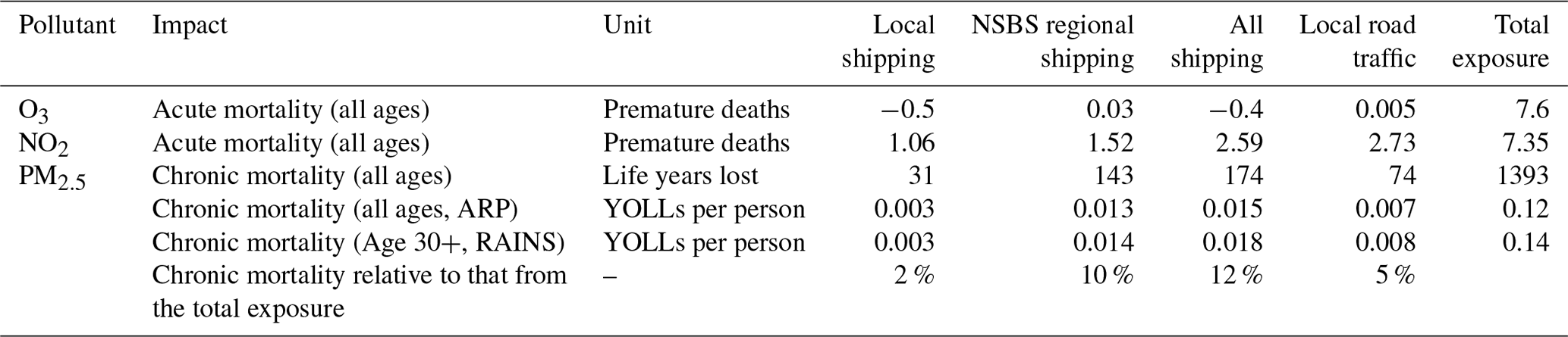
The PWCs for these pollutants were then used in the health impact calculations, and the results are presented as years of life lost per year and loss of life expectancy (years of life lost per person) for PM2.5 and as premature deaths for ozone and NO2. The estimated loss of life expectancy (YOLLs per person) due to PM2.5 from local shipping was 0.003, while from the regional shipping it was 0.014. For comparison, the impact of exposure to PM2.5 from road traffic was calculated to be 0.007 YOLLs per person and the impact of exposure to all PM2.5 in the base simulation to be 0.14 YOLLs per person (Table 3). In all, shipping contributed 12 % of the calculated health impacts from the total exposure to PM2.5 in the city and the impact was more than 2 times larger than that of local road traffic, regional shipping being a larger risk for human health than local shipping (> 80 %) in Gothenburg. The exposure to ozone related to shipping emissions reduced acute mortality by 0.4 premature deaths per year due to the NO titration effect. This effect included 0.03 additional deaths attributed to ozone formed from regional shipping emissions (Table 3). Exposure to NO2 related to shipping emissions caused 2.6 additional premature deaths yr−1, and the impact of local shipping was similar to the regional impact. This impact corresponded to 35 % of the impact of the NO2 exposure in the base simulation and was similar to the impact of road traffic.
Table 3Health impacts calculated for O3, NO2 and PM2.5 contributions of local and regional shipping and local road traffic to air pollution in the city of Gothenburg as well as of the total exposure to these pollutants in the city. The health impacts calculated with the ARP model and with the RAINS methodology are presented.
Addressing uncertainties in human health risk assessment is a critical issue when evaluating the effects of contaminants on public health due to the complex associations between environmental exposures and health. Uncertainties are introduced with the calculated pollutant concentrations, the grid resolution when assessing the population exposure, the general shape of the concentration–response function and transferability problems of the function from region to region. Hammingh et al. (2012) presented an estimate of the uncertainty in the calculations of YOLLs, which may stem from the methodology used in the YOLL calculations and from the spatial resolution. To compare the results of Jonson et al. (2015) with the results of this study, the YOLLs per person from PM2.5 exposure calculated in the ARP were multiplied by the life expectancy of the population above the age of 30, i.e. 50 years, and divided by the population in the model domain. The health impacts of PM2.5 were also calculated using the RAINS methodology directly for the calculated PM2.5 exposures. The results of both methods are presented and are very similar.
The largest uncertainties are associated with the exposure–response functions (ERFs) as such. In this study impacts for the mean values of ERFs are presented; the 95 % confidence interval for these functions is given in Sect. 2. The ERFs used here are those recommended by the WHO (2013a). For PM2.5, ERFs with higher values for spatial analyses of air pollution and mortality were found by the ESCAPE project for European cohorts (Beelen et al., 2014) as well as for mortalities in Los Angeles (Jerrett et al., 2005; 17 % per 10 µg m−3, 95 % confidence interval is 5 %–30 %). These ERFs are of very similar value, and those of Beelen et al. (2014) were used as alternative functions for estimates of broader uncertainty limits by Barregård et al. (2019). In the ARP a linear form of ERF is applied, which is justified by a rather narrow interval of PM exposure levels in Europe. In terms of the impact of the total exposure to PM2.5 on natural mortality, the linear and log-linear form of the functions give similar results within the concentration range of 10–30 µg m−3, the linear model giving slightly lower relative risks in this range and higher relative risks below and above (Ostro et. al., 2004). The PM2.5 levels found in our study fall below 10 µg m−3. For regions with high PM2.5 levels different ERF models need to be applied, and for global HIA studies or studies in other regions of the world than Western Europe and North America, ERFs for cause-specific mortalities rather than natural mortalities are usually used. There are two further important issues regarding the uncertainties associated with the ERFs. First, air pollution represents a complex mixture, and individual gases and particles are often correlated. The impacts on mortality calculated for the different pollutants therefore cannot be simply added up. Second, the ERFs assume that all particulate matter has the same impact. There is increasing evidence of different ERFs for some compounds, primarily elemental and organic carbon (WHO, 2013b).
The most robust relationship between air pollution and effects on human health is for particulate matter (WHO, 2013b). In Swedish cities, including Gothenburg, the main contribution to concentrations of PM2.5 comes from the background air (Segersson et al., 2017; Gustafsson et al., 2018). Accurate modelling of the total concentration of particulate matter is, however, very difficult as the processes affecting it are extremely complex and many of them not well quantified. These include natural and anthropogenic emissions, formation of secondary particulate matter in complex photochemical processes and dry and wet deposition processes that need to be described for the whole range of relevant geographical scales and timescales. Many regional- and global-scale models tend to underestimate the simulated PM2.5 concentrations, especially in summer, when formation of secondary PM is stronger due to the high photochemical activity, and the impact of primary PM is lower due to the more intensive mixing and smaller anthropogenic emissions of primary PM in summer (Karl et al., 2019a). Furthermore, the modelled PM concentrations used as the boundary conditions in this study showed average underestimates of PM2.5 by 60 % and 17 % in the summer and annually, respectively (Karl et al., 2019a). Two studies addressing impacts of shipping on air pollution in Gothenburg (Segersson et al., 2017; Repka et al., 2019) assessed the total concentration levels and contribution of shipping to them; however, none of them are calculated for the year 2012 assessed in this study. Segersson et al. (2017) show annual mean background PM2.5 concentrations for the year 2011 of about 5 µg m−3 for Gothenburg, reaching concentrations of >8 µg m−3 in polluted parts of the city. An annual mean concentration map presented in Repka et al. (2019) for the year 2016 shows similar concentration levels with background concentrations of about 6 µg m−3 and maximum concentrations of > 8 µg m−3. Both studies used PM10 monitoring data at the urban background station Femman to inversely derive the boundary conditions for PM2.5. Jonson et al. (2015, 2019) studied the impacts of Baltic Sea and North Sea shipping with the EMEP model for the years 2010 and 2016 and found in both cases annual mean concentration levels on the western coast of Sweden to be about 4–5 µg m−3. This concentration should correspond to the background levels of the city-scale simulations and the year 2016. Jonson et al. (2019) also compared the modelled concentrations with background measurements from the station Råö, situated 20 km south of the city, and found a model underestimation of 0.7 ppb for the annual mean. The concentration levels of PM2.5 found in this study were lower than in Segersson et al. (2017) and Repka et al. (2019), but they agree reasonably well with Jonson et al. (2015, 2019). Segersson et al. (2017) addressed the health effects of PM2.5, PM10 and black carbon in three Swedish cities, among them Gothenburg, using the Gaussian model SIMAIR. The population-weighted exposure to PM2.5 for Gothenburg was calculated to be 6.5 µg m−3, which was associated with ca. 150–290 premature deaths from exposure to PM2.5. The lower premature death number in Segersson et al. (2017) comes from calculations using the same ERF as in this study, while the higher number uses the ERF presented by Jerrett et al. (2005) for PM2.5 from the city sources. The values can be compared to the population-weighted exposure to PM2.5 of 4.1 µg m−3, associated with ca. 140 premature deaths found in this study. Jonson et al. (2015) calculated the impact of shipping emissions in the Baltic Sea and the North Sea using the EMEP model, and a map presenting the geographical distribution of life expectancy loss shows approximately 0.2 YOLLs per person around the west coast of Sweden. This agrees reasonably well with our estimate of 0.18 YOLLs per person in Gothenburg.
It is important to bear in mind the uncertainties in total concentrations of PM and other air pollutants when assessing the relative contribution of shipping to the overall impact of air pollution. Assessments of impacts of selected anthropogenic sources are, however, associated with smaller uncertainties compared to the impact of the total concentrations as some large uncertainties, e.g. those regarding the natural and agriculture sources, cancel out. The study of Segersson et al. (2017) found the contribution of shipping to the population-weighted annual PM2.5 concentration to be 0.04 µg m−3 and the contribution of road traffic exhaust emissions to be 0.27 µg m−3, which can be compared to 0.09 µg m−3 from shipping and 0.22 µg m−3 from road traffic found in this study. However, it is important to bear in mind that the studies assessed two different years.
The impact of local and regional ship emissions in the city of Gothenburg was investigated by a multi-model system for the year 2012. The model evaluation against monitoring data demonstrated fairly good agreement in meteorological parameters and acceptable estimation of hourly air pollutant concentrations.
The city-scale model simulations with and without local and regional shipping in the emission inventory revealed that the impacts from shipping on air quality in Gothenburg were substantial. The calculated contribution from local shipping to annual mean NO2 concentration was 0.5 ppb, representing 14 % of the calculated annual mean NO2 concentration. Including the contribution from regional shipping in the North Sea and the Baltic Sea, the total shipping contribution reached 1.5 ppb, representing 41 % of calculated NO2 concentrations. The contribution from regional and local shipping was higher than that from road traffic around the area of the city ports. In an analysis of exposure from different sources using population-weighted concentrations, the contribution of regional and local shipping was similar to that of road traffic in the city.
The model results of ozone concentrations have shown that titration by NO dominated the overall impact of local shipping on ozone concentration levels in Gothenburg. The maximum impact from local NOx and NMVOC emissions on summer seasonal mean ozone concentration was calculated to be −4 ppb (∼14 %). The negative effect of solely NOx emissions from local shipping on the ozone concentrations was up to −6 ppb (∼21 %) and was net negative even in the summer, when photochemical activity and potential for ozone formation are high. The emissions of NMVOC from local shipping as such increased ozone formation in the city, with the highest contribution being 2 ppb (∼7 %) as a seasonal summer mean. In terms of urban air quality control, reduction in anthropogenic NMVOC could result in a significantly greater decrease in O3 relative to the same reduction in NOx (Karl et al., 2019b).
The simulated emissions from local and regional shipping contributed an average of 0.5 µg m−3 throughout the model domain and a maximum of 1.1 µg m−3 to the annual mean concentration of PM2.5. Regional shipping is a larger contributor than local shipping to local PM2.5 concentrations, corresponding to 11 % of the local PM2.5 concentrations on average. Furthermore, its contribution to the PWC was higher, contributing 0.4 µg m−3 (10 % of the total PWC for PM2.5). Contribution from local shipping was 0.1 µg m−3 (2 % of the total).
The calculated health impacts have shown the most serious effects from shipping in Gothenburg to be associated with exposure to PM2.5. Local and regional shipping together reduce life expectancy by 0.015 years per person, of which more than 80 % is associated with regional shipping in the North Sea and the Baltic Sea. The shipping impact is more than twice as high as the modelled impact of PM2.5 associated with local road traffic. Impacts from exposure to NO2 and ozone were calculated in terms of premature deaths per year, and 2.6 additional cases yr−1 were calculated for exposure to NO2, with regional and local shipping contributing 59 % and 41 %, respectively. The impacts from exposure to ozone were of opposite magnitude. The decrease in ozone due to NO titration reduced the calculated mortalities by 0.4 cases yr−1. The impact of the exposure to PM2.5 from shipping calculated as premature deaths was 18 cases yr−1. The implementation of the more stringent SECA regulations for FSC in the year 2015 is not likely to have changed the impacts of NO2 and ozone. According to the study of Jonson et al. (2019), a reduction in the impact of the regional shipping contribution to PM2.5 of approximately 35 % could be expected around Gothenburg, while a much smaller change can be expected in emission from local shipping since hotelling and inland shipping already use a fuel with 0.1 % FSC in the model. This would mean similar reductions in the impacts related to PM2.5 in the city of Gothenburg. The global cap of 0.5 % for FSC, which entered into force on 1 January 2020, will not have any significant impact on further reduction in shipping-related air pollution in Gothenburg compared to the situation after 2015. The global study of Sofiev at al. (2018) shows that around the western coast of Sweden a decrease in PM2.5 due to the global cap would be below 1 %. The more serious health effects induced by regional shipping indicate that close cooperation across governance levels is required to effectively reduce air pollution in the city.
The impacts of local shipping emissions on air quality and human health are further discussed in Part 2 of this paper (Ramacher et al., 2020), which presents a study of several future shipping scenarios for the year 2040 that adopt changes in shipping emissions due to changes in ship traffic volumes and legislation on emissions of air pollutants at sea and on energy effectivization. These scenarios also introduce shoreside electricity in shipping.
The model output data are available upon request from the corresponding authors.
TAPM is a commercial software available from CSIRO, Australia (https://www.csiro.au/, Hurley, 2008a). STEAM is the intellectual property of the Finnish Meteorological Institute and is not publicly available. The ARP tool is intellectual property of Mike Holland and Joe Sparado (mike.holland@emrc.co.uk) and is not publicly available.
The supplement related to this article is available online at: https://doi.org/10.5194/acp-20-7509-2020-supplement.
LT, MOPR, JM and VM designed the model simulations. LJ and JPJ calculated ship emissions with STEAM and contributed text about the shipping emissions. LT prepared ship emission files for the model simulations. LT, MG and JM prepared emission data from other sources. MK and AA prepared data from the regional-scale simulation used for the boundary conditions, and MK contributed text about these simulations. LT and MOPR prepared the model set-up and other input data, performed the model simulations and evaluated the model results. LT calculated exposures, and JM and KY calculated the health impacts. LT and JM wrote the majority of the text, with assistance from MOPR and VM.
Jana Moldanová is associated editor of the special issue Shipping and Environment.
This article is part of the special issue “Shipping and the Environment – From Regional to Global Perspectives (ACP/OS inter-journal SI)”. It is not associated with a conference.
Hulda Winnes and Stefan Åström, IVL, are acknowledged for valuable comments on the manuscript. Two anonymous reviewers are gratefully acknowledged for valuable suggestions and comments.
This work resulted from the BONUS SHEBA project (grant no. 2014-41), which has received funding from BONUS (Art 185), funded jointly by the EU, the Academy of Finland, the German Federal Ministry of Education and Research (under grant no. 03F0720A) and the Swedish Environmental Protection Agency, as well as from the project platform CSHIPP, which has received funding from subsidy contract C006 of Interreg Baltic Sea Region.
This paper was edited by Huan Liu and reviewed by two anonymous referees.
Amann, M., Cofala, J., Heyes, C., Klimont, Z., Mechler, R., Posch, M., and Schöpp, W.: Documentation of the model approach prepared for the RAINS peer review 2004, Interim Report IR-04-075, 2004.
Andersson, C., Bergström, R., and Johansson, C.: Population exposure and mortality due to regional background PM in Europe – Long-term simulations of source region and shipping contributions, Atmos. Environ., 43, 3614–3620, 2009.
Åström, S., Yaramenka, K., Winnes, H., Fridell, E., and Holland, M.: The costs and benefits of a nitrogen emission control area in the Baltic and North Seas, Transport. Res. D, 59, 223–236, 2018.
Aulinger, A., Matthias, V., Zeretzke, M., Bieser, J., Quante, M., and Backes, A.: The impact of shipping emissions on air pollution in the greater North Sea region – Part 1: Current emissions and concentrations, Atmos. Chem. Phys., 16, 739–758, https://doi.org/10.5194/acp-16-739-2016, 2016.
Azzi, M., Johnson, G. M., and Cope, M.: An introduction to the generic reaction set photochemical smog mechanism, Proceedings of the 11th International Clean Air and Environment Conference, Brisbane, 1992, Clean Air Society of Australia & New Zealand, 1992.
Barregård, L., Molnár, P., Jonson, J.-E., and Stockfelt, L.: Impact on population health of Baltic shipping Emissions, Int. J. Environ. Res. Pu., 16, 1954, https://doi.org/10.3390/ijerph16111954, 2019.
Beelen, R., Raaschou-Nielsen, O., Stafoggia, M., Andersen, Z.J., Weinmayr, G., Hoffmann, B., Wolf, K., Samoli, E., Fischer, P., Nieuwenhuijsen, M., Vineis, P., Xun, W.W., Katsouyanni, K., Dimakopoulou, K., Oudin, A., Forsberg, B., Modig, L., Havulinna, A.S., Lanki, T., Turunen, A., Oftedal, B., Nystad, W., Nafstad, P., De Faire, U., Pedersen, N.L., Östenson, C.G., Fratiglioni, L., Penell, J., Korek, M., Pershagen, G., Eriksen, K.T., Overvad, K., Ellermann, T., Eeftens, M., Peeters, P.H., Meliefste, K.,Wang, M., Bueno-De-Mesquita, B., Sugiri, D., Krämer, U., Heinrich, J., De Hoogh, K., Key, T., Peters, A., Hampel, R., Concin, H., Nagel, G., Ineichen, A., Scha?ner, E., Probst-Hensch, N., Künzli, N., Schindler, C., Schikowski, T., Adam, M., Phuleria, H., Vilier, A., Clavel-Chapelon, F., Declercq, C., Grioni, S., Krogh, V., Tsai, M.Y., Ricceri, F., Sacerdote, C., Galassi, C., Migliore, E., Ranzi, A., Cesaroni, G., Badaloni, C., Forastiere, F., Tamayo, I., Amiano, P., Dorronsoro, M., Katsoulis, M., Trichopoulou, A., Brunekreef, B., and Hoek, G.: Effects of long-term exposure to air pollution on natural-cause mortality: an analysis of 22 European cohorts within the multicentre ESCAPE project, Lancet, 383, 785–795, https://doi.org/10.1016/S0140-6736(13)62158-3, 2014.
Bieser, J., Aulinger, A., Matthias, V., Quante, M., and Builtjes, P.: SMOKE for Europe – adaptation, modification and evaluation of a comprehensive emission model for Europe, Geosci. Model Dev., 4, 47–68, https://doi.org/10.5194/gmd-4-47-2011, 2011.
Byun, D. and Ching, J.: Science Algorithms of the EPA Models-3 Community Multiscale Air Quality Modeling System, Epa/600/r-99/030, US Environmental Protection Agency, Office of Research and Development, Washington DC, 1999.
Byun, D. and Schere, K.: Review of the Governing Equations, Computational Algorithms, and Other Components of the Models-3 Community Multiscale Air Quality (CMAQ) Modeling System, Appl. Mech. Rev., 59, 51–77, 2006.
CEIP: WebDab – EMEP database, available at: http://www.ceip.at/emission-data-webdab/emissions-used-in-emep-models/, last access: 7 October 2018.
Cofala, J., Amann, M., Heyes, C., Wagner, F., Klimont, Z., Posch, M., Schöpp, W., Tarasson, L., Jonson, J. E., Whall, C., and Stavrakaki, A.: Analysis of policy measures to reduce ship emissions in the context of the revision of the National Emissions Ceilings Directive, IIASA report, No. 06-107, 2007.
Corbett, J. J., Fischbeck, P. S., and Pandis, S. N.: Global nitrogen and sulfur inventories for oceangoing ships, J. Geophys. Res., 104, 3457–3470, 1999.
EPER: European Pollutant Emission Register, available at: https://www.eea.europa.eu/data-and-maps/data/ member-states-reporting-art-7-under-the-european-pollutant-release-and-transfer-register-e-prtr-regulation-16, last access: 7 February 2018.
Eyring, V., Köhler, H.W., van Aardenne, J., and Lauer, A.: Emissions from international shipping: 1. The last 50 years, J. Geophys. Res., 110 D17305, https://doi.org/10.1029/2004JD005620, 2005.
Fridell, E., Haeger-Eugensson, M., Moldanova, J., Forsberg, B., and Sjöberg, K.: A modeling study of the impact on air quality and health due to the emissions from E85 and petrol fueled cars in Sweden, Atmos. Environ., 82, 1–8, 2014.
Gustafsson, M., Lindén, J., Tang, L., Forsberg, B., Orru, H., Åström, S., and Sjöberg, K.: Quantificaiton of population exposure to NO2, PM2.5 and PM10 and estimated health impacts, IVL report, No. C317, 2018.
Hammingh, P., Holland, M. R., Geilenkirchen, G. P., Jonson, J. E., and Maas, R. J. M.: Assessment of the Environmental Impacts and Health Benefits of a Nitrogen Emission Control Area in the North Sea. Policy studies PBL Netherlands Environmental Assessment Agency (PBL), The Hague, p. 113, 2012.
Holland, M. R., Pye, S., and Jones, G.: EC4MACS Modelling Methodology-The ALPHA Benefit Assessment Model, European Consortium for Modelling of Air Pollution and Climate Strategies – EC4MACS, 2013.
Hurley, P.: TAPM v. 4. User Manual, CSIRO, ISBN 978-1-921424-73-1, 2008a.
Hurley, P.: TAPM v. 4. Part 1: Technical Description, CSIRO, ISBN 978-1-921424-71-7, 2008b.
Hurley, P., Physick, W., and Luhar, A.: TAPM – a practical approach to prognostic meteorological and air pollution modelling, Environ. Modell. Softw., 20, 737–752, https://doi.org/10.1016/j.envsoft.2004.04.006, 2005.
Huszar, P., Cariolle, D., Paoli, R., Halenka, T., Belda, M., Schlager, H., Miksovsky, J., and Pisoft, P.: Modeling the regional impact of ship emissions on NOx and ozone levels over the Eastern Atlantic and Western Europe using ship plume parameterization, Atmos. Chem. Phys., 10, 6645–6660, https://doi.org/10.5194/acp-10-6645-2010, 2010.
Jalkanen, J.-P., Brink, A., Kalli, J., Pettersson, H., Kukkonen, J., and Stipa, T.: A modelling system for the exhaust emissions of marine traffic and its application in the Baltic Sea area, Atmos. Chem. Phys., 9, 9209–9223, https://doi.org/10.5194/acp-9-9209-2009, 2009.
Jalkanen, J.-P., Johansson, L., Kukkonen, J., Brink, A., Kalli, J., and Stipa, T.: Extension of an assessment model of ship traffic exhaust emissions for particulate matter and carbon monoxide, Atmos. Chem. Phys., 12, 2641–2659, https://doi.org/10.5194/acp-12-2641-2012, 2012.
Jerrett, M., Burnett, R. T., Ma, R. J., Pope, C. A., Krewski, D., Newbold, K. B., Thurston, G., Shi, Y., Finkelstein, N., Calle, E. E., and Thun, M. J.: Spatial analysis of air pollution and mortality in Los Angeles, Epidemiology, 16, 727–736, 2005.
Johansson, L., Jalkanen, J.-P., and Kukkonen, J.: Global assessment of shipping emissions in 2015 on a high spatial and temporal resolution, Atmos. Environ., 167, 403–415, https://doi.org/10.1016/j.atmosenv.2017.08.042, 2017.
Jonson, J. E., Jalkanen, J. P., Johansson, L., Gauss, M., and Denier van der Gon, H. A. C.: Model calculations of the effects of present and future emissions of air pollutants from shipping in the Baltic Sea and the North Sea, Atmos. Chem. Phys., 15, 783–798, https://doi.org/10.5194/acp-15-783-2015, 2015.
Jonson, J. E., Gauss, M., Jalkanen, J.-P., and Johansson, L.: Effects of strengthening the Baltic Sea ECA regulations, Atmos. Chem. Phys., 19, 13469–13487, https://doi.org/10.5194/acp-19-13469-2019, 2019.
Karl, M.: Development of the city-scale chemistry transport model CityChem-EPISODE and its application to the city of Hamburg, Geosci. Model Dev. Discuss., https://doi.org/10.5194/gmd-2018-8, 2018.
Karl, M., Jonson, J. E., Uppstu, A., Aulinger, A., Prank, M., Sofiev, M., Jalkanen, J.-P., Johansson, L., Quante, M., and Matthias, V.: Effects of ship emissions on air quality in the Baltic Sea region simulated with three different chemistry transport models, Atmos. Chem. Phys., 19, 7019–7053, https://doi.org/10.5194/acp-19-7019-2019, 2019a.
Karl, M., Walker, S.-E., Solberg, S., and Ramacher, M. O. P.: The Eulerian urban dispersion model EPISODE – Part 2: Extensions to the source dispersion and photochemistry for EPISODE–CityChem v1.2 and its application to the city of Hamburg, Geosci. Model Dev., 12, 3357–3399, https://doi.org/10.5194/gmd-12-3357-2019, 2019b.
Karl, M., Bieser, J., Geyer, B., Matthias, V., Jalkanen, J.-P., Johansson, L., and Fridell, E.: Impact of a nitrogen emission control area (NECA) on the future air quality and nitrogen deposition to seawater in the Baltic Sea region, Atmos. Chem. Phys., 19, 1721–1752, https://doi.org/10.5194/acp-19-1721-2019, 2019c.
Landmäteriet: Kartor och geografisk information, available at: https://www.lantmateriet.se/sv/Kartor-och-geografisk-information/gps-geodesi-och-swepos/referenssystem/tvadimensionella-system/sweref-99-projektioner/, last access: 11 June 2020.
Matthias, V., Aulinger, A., Backes, A., Bieser, J., Geyer, B., Quante, M., and Zeretzke, M.: The impact of shipping emissions on air pollution in the greater North Sea region – Part 2: Scenarios for 2030, Atmos. Chem. Phys., 16, 759–776, https://doi.org/10.5194/acp-16-759-2016, 2016.
Miljöförvaltningen: Luftkvaliteten i Göteborgsområdet Årsrapport 2016 R2017:06, ISBN 1401-2448, 2017.
Miller, B. G. and Hurley, J. F.: Life table methods for quantitative impact assessments in chronic mortality, J. Epidemiol. Commun. H., 57, 200–206, 2003.
Molnár, P., Tang, L., Sjöberg, K., and Wichmann, J.: Long-range transport clusters and positive matrix factorization source apportionment for investigating transboundary PM2.5 in Gothenburg, Sweden, Environ. Sci.-Proc. Imp., 19, 1270–1277, https://doi.org/10.1039/C7EM00122C, 2017.
Olivier, J. G. J., Bouwman, A. F., Berdowski, J. J. M., Veldt, C., Bloos, J. P. J., Visschedijk, A. J. H., Van der Maas, C. W. M., and Zandveld, P. Y. J.: Sectoral emission inventories of greenhouse gases for 1990 on a per country basis as well as on , Environ. Sci. Policy, 2, 241–264, 1999.
Olstrup, H., Forsberg, B., Orru, H., Spanne, M., Nguyen, H., Molnár, P., and Johansson, C.: Trends in air pollutants and health impacts in three Swedish cities over the past three decades, Atmos. Chem. Phys., 18, 15705–15723, https://doi.org/10.5194/acp-18-15705-2018, 2018.
Ostro, B.: Outdoor air pollution: Assessing the environmental burden of disease at national and local levels. WHO Environmental Burden of Disease Series, No. 5, Geneva, WHO, 2004.
Pernigotti, D., Gerboles, M., and Thunis, P.: Modeling quality objectives in the framework of the FAIRMODE project: working document, FAIRMODE webpage, available at: https://fairmode.jrc.ec.europa.eu/, last access: 12 June 2020.
Pope, C. A., Burnett, R. T., Thun, M. J., Calle, E. E., Krewski, D., Ito, K., and Thurston, G. D.: Lung cancer, cardiopulmonary mortality, and long-term exposure to fine particulate air pollution, J. Am. Med. Assoc., 287, 1137–1141, 2002.
Ramacher, M. O. P.: Performance and evaluation of local scale wind flow fields for urban air pollution modeling with the coupled prognostic model TAPM driven by ERA5 climate reanalysis data, Geophys. Res. Abstr., 20, EGU2018-8112, https://meetingorganizer.copernicus.org/EGU2018/EGU2018-8112.pdf (last access: 26 June 2020), 2018.
Ramacher, M. O. P., Karl, M., Bieser, J., Jalkanen, J.-P., and Johansson, L.: Urban population exposure to NOx emissions from local shipping in three Baltic Sea harbour cities – a generic approach, Atmos. Chem. Phys., 19, 9153–9179, https://doi.org/10.5194/acp-19-9153-2019, 2019.
Ramacher, M. O. P., Tang, L., Moldanová, J., Matthias, V., Karl, M., Fridell, E., and Johansson, L.: The impact of ship emissions on air quality and human health in the Gothenburg area – Part II: Scenarios for 2040, Atmos. Chem. Phys. Discuss., https://doi.org/10.5194/acp-2020-319, in review, 2020.
Repka, S., Mellqvist, J., Borkowski, T., Jalkanen, J.-P., Jonson, J. E., Barregard, L., Olaniyi, E., Prause, G. K., Gauss, M., Walden, J., Svensson, E., Genikhovich, E., Rumyantzev, D., Boyesen, J., Wenske, C., de Carvalho, T. P., Lähteenmäki-Uutela, A., Johansson, L., Conde, V., Erkkilä-Välimäki, A., Yliskylä-Peuralahti, J., Saarnio, K., Bakhtov, A., Tochanskaya, S., Bosch, M., Haukioja, T., Törrönen, J., Karppinen, A., Beecken, J., Alhosalo, M., Myskow, J., Kowalak, P., Bäck, E., Nguyen, H., Molnar, P., Stockfelt, L., Atari, S., and Bakkar, Y.: EnviSuM, Clean Shipping: Exploring the impact of emission regulation, Final report, available at: https://blogit.utu.fi/envisum/ (last access: 12 June 2020), 2019.
Rexeis, M., Hausberger, S., Kühlwein, J., and Luz, R.: Update of Emission Factors for EURO 5 and EURO 6 vehicles for the HBEFA Version 3.2, Report No. I-31/2013/ Rex EM-I 2011/20/679 from 06.12.2013, Graz University of Technology, Switzerland, available at: https://www.hbefa.net/d/documents/HBEFA32_EF_Euro_5_6_TUG.pdf (last access: 11 June 2020), 2013.
Rockel, B., Will, A., and Hense, A.: The Regional Climate Model COSMO-CLM (CCLM), Metz, 17, 347–348, https://doi.org/10.1127/0941-2948/2008/0309, 2008.
Segersson, D., Eneroth, K., Gidhagen, L., Johansson, C., Omstedt, G., Nylén, A. E., and Fosberg, B.: Health impact of PM10, PM2.5 and black carbon exposure due to different source sectors in Stockholm, Gothenburg and Umea, Sweden, Int. J. Environ. Res. Pu., 14, 742, https://doi.org/10.3390/ijerph14070742, 2017.
SMED: Description of Methods and Quality of Spatially Distributed Emissions to Air, Contract no. 309, 1235, 2015.
Sofiev, M., Siljamo, P., Valkama, I., Ilvonen, M., and Kukkonen, J.: A dispersion mod-elling system SILAM and its evaluation against ETEX data, Atmos. Environ., 40, 674–685, 2006.
Sofiev, M., Winebrake, J. J., Johansson, L., Carr, E. W., Prank, M., Soares, J., Vira, J., Kouznetsov, R., Jalkanen J.-P., and Corbett, J. J.: Cleaner fuels for ships provide public health benefits with climate tradeoff, Nat. Commun., 9, p. 406, https://doi.org/10.1038/s41467-017-02774-9, 2018.
Thunis, P., Pederzoli, A., and Pernigotti, D.: Performance criteria to evaluate air quality modeling applications, Atmos. Environ., 79, 476–482, 2012.
Winnes, H., Styhre, L., and Fridell, E.: Reducing GHG emissions from ships in port areas, Res. Trans. Bus. Manage., 17, 73–82, 2015.
WHO: Health risks of air pollution in Europe – HRAPIE project: Recommendations for concentration–response functions for cost–benefit analysis of particulate matter, ozone and nitrogen dioxide, available at: http://www.euro.who.int/ (last access: 21 October 2019), 2013a.
WHO: Review of evidence on health aspects of air pollution – REVIHAAP project: final technical report, available at: https://www.euro.who.int/__data/assets/pdf_file/0004/193108/REVIHAAP-Final-technical-report-final-version.pdf (last access: 12 June 2020), 2013b.
- Abstract
- Copyright statement
- Introduction
- Methodology
- Results and discussion
- Calculation of exposure and health effects from ship emissions
- Assessment of uncertainties and comparison with other studies
- Conclusions
- Data availability
- Code and data availability
- Author contributions
- Competing interests
- Special issue statement
- Acknowledgements
- Financial support
- Review statement
- References
- Supplement