the Creative Commons Attribution 4.0 License.
the Creative Commons Attribution 4.0 License.
 | 25 Jun 2020
Microphysics and dynamics of snowfall associated with a warm conveyor belt over Korea
Josué Gehring
Annika Oertel
Étienne Vignon
Nicolas Jullien
Nikola Besic
On 28 February 2018, 57 mm of precipitation associated with a warm conveyor belt (WCB) fell within 21 h over South Korea. To investigate how the large-scale circulation influenced the microphysics of this intense precipitation event, we used radar measurements, snowflake photographs and radiosounding data from the International Collaborative Experiments for Pyeongchang 2018 Olympic and Paralympic Winter Games (ICE-POP 2018). The WCB was identified with trajectories computed with analysis wind fields from the Integrated Forecast System global atmospheric model. The WCB was collocated with a zone of enhanced wind speed of up to 45 m s−1 at 6500 m a.s.l., as measured by a radiosonde and a Doppler radar. Supercooled liquid water (SLW) with concentrations exceeding 0.2 g kg−1 was produced during the rapid ascent within the WCB. During the most intense precipitation period, vertical profiles of polarimetric radar variables show a peak and subsequent decrease in differential reflectivity as aggregation starts. Below the peak in differential reflectivity, the specific differential phase shift continues to increase, indicating early riming of oblate crystals and secondary ice generation. We hypothesise that the SLW produced in the WCB led to intense riming. Moreover, embedded updraughts in the WCB and turbulence at its lower boundary enhanced aggregation by increasing the probability of collisions between particles. This suggests that both aggregation and riming occurred prominently in this WCB. This case study shows how the large-scale atmospheric flow of a WCB provides ideal conditions for rapid precipitation growth involving SLW production, riming and aggregation. Future microphysical studies should also investigate the synoptic conditions to understand how observed processes in clouds are related to large-scale circulation.
- Article
(11649 KB) - Full-text XML
- BibTeX
- EndNote


Precipitation is the result of a chain of meteorological processes ranging from synoptic to microscales. In particular for stratiform precipitation, large-scale flow drives the transport of moisture and lifting of air masses, while microphysics ultimately determines the growth and fall of hydrometeors, influencing precipitation intensity and accumulation. Therefore understanding the link between large-scale flow and microphysics is paramount to better forecasting precipitation. Extratropical cyclones are the main synoptic-scale features associated with precipitation at mid-latitudes and produce more than 80 % of the total precipitation in the Northern Hemisphere storm tracks (Hawcroft et al., 2012). Quasi-Lagrangian analyses of mid-latitude baroclinic storms have shown the existence of three distinctive airstreams (Carlson, 1980): the dry intrusion, the cold conveyor belt (Harrold, 1973; Browning, 1990; Schultz, 2001) and the warm conveyor belt (WCB; Green et al., 1966; Harrold, 1973; Browning et al., 1973; Dacre et al., 2019; Wernli and Knippertz, 2020). The latter can be defined as a coherent warm and moist airstream rising from the boundary layer to the upper troposphere in about 2 d (Eckhardt et al., 2004; Madonna et al., 2014). Climatological studies of WCBs have used a simple criterion on the ascent rate of trajectories (e.g. 600 hPa in 48 h; Madonna et al., 2014).
WCBs typically rise from below 900 to about 300 hPa, and temperature along this flow typically decreases from above 0 to below −40 ∘C. Therefore, clouds along WCBs feature the whole spectrum from warm clouds to mixed-phase to pure-ice clouds (e.g. Joos and Wernli, 2012; Madonna et al., 2014). WCBs are the primary precipitation-producing feature in extratropical cyclones (Browning, 1990; Eckhardt et al., 2004) and are responsible for more than 70 % of precipitation extremes in the major storm tracks (Pfahl et al., 2014). However, precipitation and cloud processes also impact the dynamics of extratropical cyclones. Trajectory analyses have shown that WCBs experience a strong cross-isentropic ascent due to latent heat release (Madonna et al., 2014), which leads to an increase in potential vorticity (PV) below the maximum diabatic heating level and a decrease above it (Wernli and Davies, 1997). This represents a direct link between microphysics and dynamics. Joos and Wernli (2012) studied the impact of different microphysical processes on the diabatic PV production in WCBs. They suggested that condensation of cloud liquid and depositional growth of snow and ice are the most significant diabatic heating processes in WCBs. Joos and Forbes (2016) showed the direct impact of specific microphysical processes on PV modification in WCBs and the subsequent downstream flow evolution.
Colle et al. (2014) studied the distribution of snow crystal habits within mid-latitude baroclinic storms over Long Island, New York. They observed moderately rimed crystals in the middle of the comma head, while heavy riming was present close to the cyclone centre. They also showed a positive correlation between vertical wind speeds, turbulence and degree of riming by means of Doppler data from a micro rain radar. Overall, this study highlights the spatial structure of microphysics occurring in winter storms and suggests a link between the dynamics of the cyclone and observed snow crystal habits.
Dual-polarisation Doppler (polarimetric) radars are useful to study precipitation microphysics as they provide information on the hydrometeors' shape, density and phase. For instance, differential reflectivity ZDR, defined as the logarithmic ratio between the reflectivity factor at horizontal and vertical polarisations (ZH−ZV in decibels), is a measure of the reflectivity-weighted axis ratio of the targets (Kumjian, 2013; Bringi and Chandrasekar, 2001). Oblate particles (e.g. raindrops and dendrites) have positive ZDR values, while prolate ones (e.g. vertically oriented ice in an electric field) exhibit negative ZDR values. ZDR also depends on the crystal's dielectric constant but not on the number concentration. Therefore, large aggregates tend to have small ZDR values (<0.5 dB; Kumjian, 2013) primarily because they have a much lower density than solid ice but also because they tend to be more spherical than pristine crystals. On the other hand, aggregates are much larger than crystals and tend to have higher ZH values. Consequently, decreasing ZDR together with increasing ZH towards the ground is a consistent signature of the aggregation process (Schneebeli et al., 2013; Kumjian et al., 2014; Grazioli et al., 2015). Furthermore, the specific differential phase shift (Kdp; in degrees per kilometre), which is the range derivative of the total differential phase shift on propagation (i.e. phase difference between the horizontal and vertical polarisation waves propagating forward), is related to the axis ratio, the density, the number concentration and the size of the targets. Being a lower-order moment than ZH, it is more influenced by the number concentration such that a high number concentration of small oblate crystals can lead to an increase in Kdp, while ZDR will barely be affected. Owing to this wealth of information, polarimetric variables have been extensively used for snowfall microphysical studies (Bader et al., 1987; Andrić et al., 2013; Schneebeli et al., 2013; Moisseev et al., 2015; Grazioli et al., 2015). The pioneering work of Bader et al. (1987) showed that high ZDR values are associated with large dendritic crystals. More recently, Moisseev et al. (2015) found that enhanced values of specific differential phase (Kdp) are related to the onset of aggregation, producing early aggregates that can be oblate. Grazioli et al. (2015) suggested that similar peaks in Kdp can result from secondary ice generation (leading to a high number concentration of small anisotropic crystals) or the riming of oblate ice crystals, which increases their density. These studies thoroughly analysed dual-polarisation signatures of snowfall microphysics. However, they did not consider the interactions between large-scale flow and microphysics. Keppas et al. (2018) studied the microphysical properties of a warm front with radar and in situ measurements in clouds. They found that a WCB formed a widespread mixed-phase cloud by producing a significant amount of liquid water, which favoured riming and secondary ice generation. However, they did not formally identify WCB trajectories nor did they confirm that the liquid water was produced within the WCB. There is hence a need to better understand how the strong, coherent ascending motion within WCBs influences precipitation microphysics. To this end, a synergy between remote-sensing and in situ measurements as well as trajectory analyses is needed.
In this study, we use data from the International Collaborative Experiments for Pyeongchang 2018 Olympic and Paralympic Winter Games (ICE-POP 2018) campaign to study an extreme snowfall event associated with a WCB over South Korea on 28 February 2018. The location of Pyeongchang on a peninsula at mid-latitudes offers an interesting setting to study the interplay between synoptic circulation, orographic effects and microphysics. First, the surrounding Yellow Sea and East Sea provide nearby sources of moisture for precipitation, which is particularly relevant for wintertime WCBs (Pfahl et al., 2014). Secondly, WCBs play a crucial role for precipitation over the Korean Peninsula: between 80 % and 90 % of extreme precipitation is associated with WCBs in South Korea according to a climatological study by Pfahl et al. (2014). The ICE-POP 2018 data set includes, among other data, multiple-frequency radar measurements and high-resolution snowflake photographs. We also make use of the Integrated Forecast System (IFS; ECMWF, 2017) model from the European Centre for Medium-Range Weather Forecasts to identify WCB trajectories associated with this event.
To understand the role of the WCB during this intense precipitation event in Korea, we address the following questions:
-
What was the synoptic situation leading to this intense snowfall event?
-
Which microphysical processes were involved?
-
How did the specific flow conditions in the WCB influence the observed microphysics?
The paper is structured as follows. We first introduce the measurement campaign and data sets in Sect. 2. The synoptic situation is presented in Sect. 3. Section 4 shows the evolution of the event over Pyeongchang. An analysis of the microphysics observed by radar and snowflake images during succeeding periods of interest is presented in Sect. 5. We then summarise the key findings of this study with a conceptual model in Sect. 6 before concluding in Sect. 7.
ICE-POP 2018 was a measurement campaign organised by the Korea Meteorological Administration and supported by the World Meteorological Organisation. Figure 1 shows the location of Pyeongchang and the measurement sites. One of the main goals of ICE-POP 2018 was to improve our understanding of orographic precipitation in the Taebaek mountains (the mountain range along the east coast of the Korean Peninsula in Fig. 1). For this purpose, remote-sensing and in situ measurements of clouds and precipitation were conducted in the Pyeongchang and Gangneung provinces between November 2017 and May 2018. In this study, we focus on the data collected by an X-band Doppler dual-polarisation radar (hereafter MXPol), a W-band Doppler cloud profiler (hereafter WProf) and a multi-angle snowflake camera (hereafter MASC), details of which are provided in the following subsections. In addition, we use measurements from a Pluvio2 weighing rain gauge located at the Mayhills site (MHS; Fig. 1). Finally, we show radiosondes (3-hourly resolution) and temperature measurements from Daegwallyeong (DGW), located 2 km away from MHS.
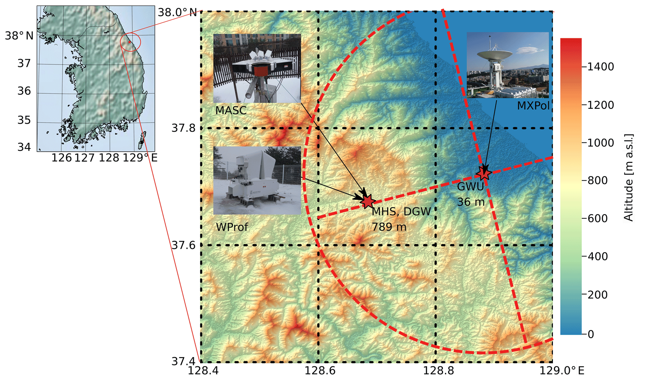
Figure 1Location of the main measurement sites of ICE-POP 2018 used in this study. A digital elevation model shows the topography of the region and its location within South Korea. The dotted red lines and circle show the extent of the main RHIs (27.2 km) and the PPI (28.4 km radius), respectively.
2.1 X-band Doppler dual-polarisation radar
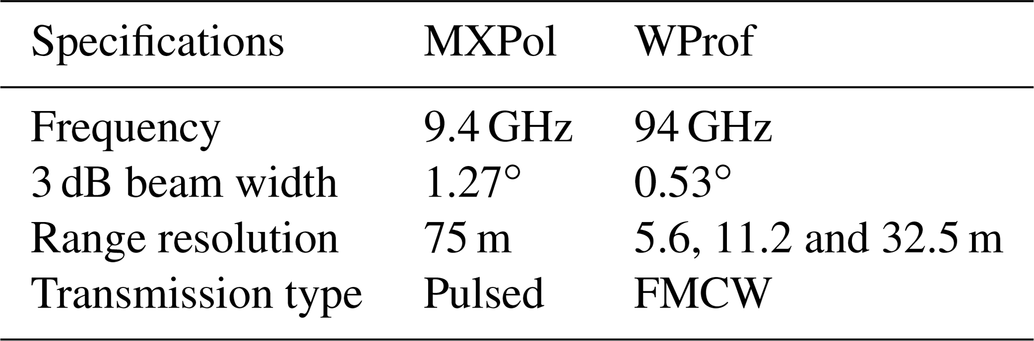
MXPol was installed on top of a building at Gangneung–Wonju National University (GWU) at the coast of the East Sea (Fig. 1). MXPol operates at 9.41 GHz with a typical angular resolution of 1∘, range resolution of 75 m, non-ambiguous range of 28 km and a Nyquist velocity of 39 m s−1 in dual-pulse pair (DPP) mode or 11 m s−1 in fast Fourier transform (FFT) mode (see Schneebeli et al., 2013, for more details). The scan cycle was composed of three hemispherical range height indicators (RHIs) at 225.8∘ (in FFT), 233∘ (in DPP) and 325.7∘ (in DPP) azimuth. The first two are towards MHS, while the third is perpendicular to this direction following the coast (dashed red lines in Fig. 1). The RHIs were performed with a range resolution of 75 m and an extent of 27.2 km. The cycle was completed by one plan position indicator (PPI) in DPP mode at 6∘ elevation (dashed red circle in Fig. 1) and one PPI in FFT mode at 90∘ elevation (for ZDR monitoring). The PPI at 6∘ elevation had a range resolution of 75 m and an extent of 28.4 km. The scan cycle had a 5 min duration and was repeated indefinitely. The main variables retrieved from MXPol measurements are the reflectivity factor at horizontal polarisation ZH (dBZ), ZDR (dB), Kdp (), the mean Doppler velocity (m s−1) and the Doppler spectral width SW (m s−1). During the FFT scans the full Doppler spectrum at 0.17 m s−1 resolution was retrieved. A semi-supervised hydrometeor classification (Besic et al., 2016) was applied to the polarimetric variables. A recently developed demixing module of this method (Besic et al., 2018) was also used to estimate the proportions of hydrometeor classes within one radar volume, which allows us to study mixtures of hydrometeors.
2.2 W-band Doppler cloud profiler
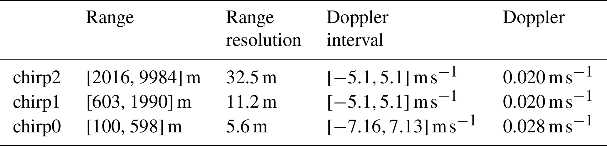
WProf was deployed at MHS, 19 km inland from GWU at 789 m a.s.l. WProf is a frequency-modulated continuous-wave (FMCW) radar operating at 94 GHz used to sample the vertical column above the radar using typically three vertical chirps (Table 1). It consists of one transmitting and one receiving antenna. A comparison of MXPol and WProf specifications can be found in Table 2. WProf has an integrated passive radiometer at 89 GHz, which provides the brightness temperature of the vertical column above the radar (see Küchler et al., 2017, for more details).
2.3 Multi-angle snowflake camera
The MASC was deployed in a double-fence wind shield at MHS. It is composed of three coplanar cameras separated by an angle of 36∘. As hydrometeors fall in the triggering area, high-resolution stereographic pictures are taken, and their fall speed is measured. A complete description of the MASC can be found in Garrett et al. (2012). The MASC images were used as input parameters to a solid-hydrometeor classification algorithm. Each individual particle is classified into six solid-hydrometeor types, namely small particles (SPs), columnar crystal (CC), planar crystal (PC), a combination of column and plate crystal (CPC), aggregate (AG), and graupel (GR). In addition, the maximum dimension (diameter of the circumscribed circle) of particles is measured to characterise the size of the snowflakes. A detailed explanation of the algorithm is provided in Praz et al. (2017). One challenge during the measurement of snowflakes in free fall is the contamination from blowing snow. Schaer et al. (2020) developed a method to automatically identify blowing snow particles in MASC images. Despite the presence of a double-fence wind shield during ICE-POP 2018, 31 % of the particles were identified as blowing snow and removed for this study. We make use of particle size distributions estimated from the maximum diameter of particles following the work of Jullien et al. (2019).
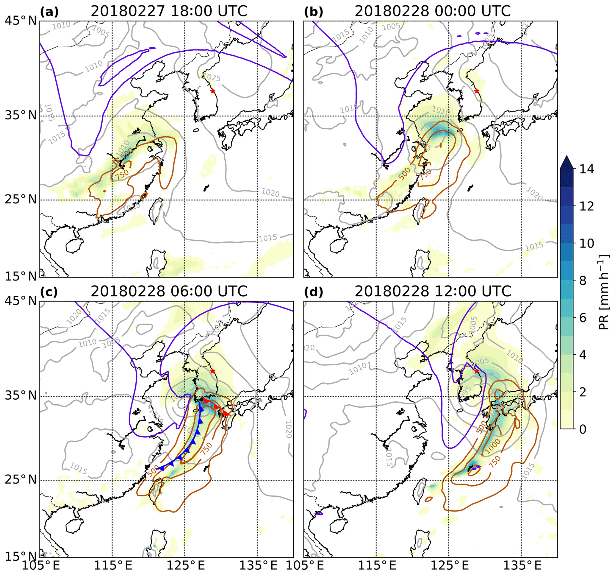
Figure 2Sea level pressure (grey contours, labels in hectopascals), dynamical tropopause on the 315 K isentrope (purple lines), IVT (brown contours, labels in kilograms per metre per second; only values greater than 500 are shown) and precipitation rate (PR) in millimetres per hour (colour-filled) at (a) 18:00 UTC on 27 February 2018 and (b) 00:00 UTC, (c) 06:00 UTC and (d) 12:00 UTC on 28 February 2018 from ERA5 data. The warm and cold fronts at 06:00 UTC were manually drawn based on an analysis of equivalent potential temperature at 850 hPa. The red star shows the location of GWU.
2.4 Warm conveyor belt trajectory computation
We define the large-scale WCB ascent over the Korean Peninsula from a Lagrangian perspective as a coherent ensemble of trajectories with an ascent rate of at least 600 hPa in 48 h (Wernli and Davies, 1997; Madonna et al., 2014). The 48 h trajectories were computed with the Lagrangian analysis tool LAGRANTO (Wernli and Davies, 1997; Sprenger and Wernli, 2015) based on the 1-hourly 3D wind field of the hydrostatic model IFS (model version Cy43r3, operational from July 2017 to June 2018; ECMWF, 2017). The details of the microphysics scheme can be found in Forbes et al. (2011). The IFS is run with a spatial resolution of O1280 (approximately 9 km) and 137 vertical hybrid pressure–sigma levels (ECMWF, 2017). The IFS data set combines operational analyses at 00:00, 06:00, 12:00 and 18:00 UTC with hourly short-term forecasts in between. The data set was interpolated to a latitude–longitude grid with 0.5∘ spatial resolution for trajectory computation. To analyse the air parcel ascent in the vicinity of the measurement site, we combine 24 h backward and 24 h forward trajectories starting every hour between 00:00 UTC on 27 February and 00:00 UTC on 1 March 2018 every 50 hPa from 1000 to 200 hPa in the proximity of Pyeongchang. WCB trajectories are subsequently selected as trajectories exceeding an ascent rate of 600 hPa in 48 h. In addition to this Lagrangian representation (i.e. following the trajectories), we projected the WCB trajectories in an Eulerian reference frame above Pyeongchang. This gives for each time step and for all vertical levels the position of trajectories above Pyeongchang which ascended with ascent rates of at least 600 hPa in 48 h within the period between 00:00 UTC on 27 February and 00:00 UTC on 1 March 2018. This highlights the heights at which WCB air parcels (i.e. with strong ascent at any given time) occur.
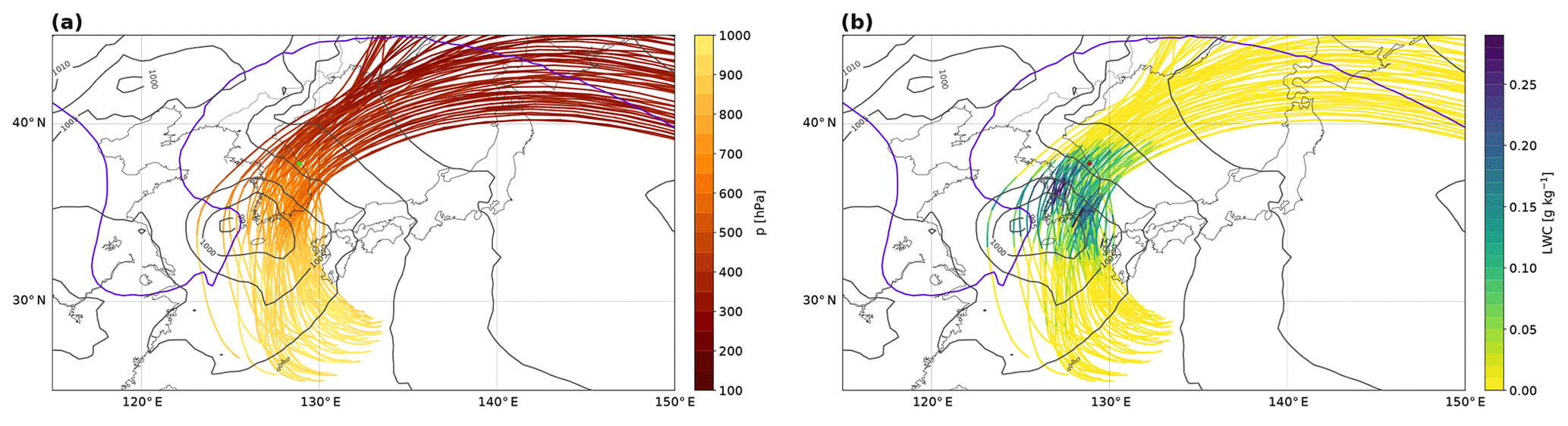
Figure 3WCB trajectories with an ascent rate of at least 600 hPa in 48 h that are located near the measurement site at 06:00 UTC on 28 February 2018. Colours indicate (a) the pressure level and (b) the LWC along the WCB air parcels. Also shown are sea level pressure (grey contours, every 5 hPa) and the dynamical tropopause at 315 K (purple). Only the WCB trajectories close to the site (green asterisk in panel a and red in panel b) are shown.
The 28 February 2018 precipitation event is the most intense of the whole ICE-POP 2018 campaign. It contributed 77 % of the winter 2018 (December–February) precipitation accumulation. At 18:00 UTC on 27 February 2018 (Fig. 2a) a PV streamer (equatorwards excursion of stratospheric air) was located over eastern China and moved eastward towards South Korea. At 00:00 UTC on 28 February 2018 (Fig. 2b) a surface cyclone formed in the Yellow Sea east of the upper-level PV streamer. Around 06:00 UTC, the surface cyclone intensified as the PV streamer was approaching (Fig. 2c) and became fully developed with a cold front passing to the south of the Korean Peninsula and a warm front passing over Pyeongchang. The interaction between the upper-level PV streamer and the surface cyclone led to a rapid deepening of the cyclone by 25 hPa between 18:00 UTC on 27 February and 12:00 UTC on 28 February. The integrated vapour transport (IVT; Rutz et al., 2014) contours show the strong moisture flux ahead of the cold front, with the most intense precipitation close to the cyclone centre, where the IVT gradient is the largest. At 12:00 UTC the cyclone moved further east, and the PV streamer was located over Korea, inducing an increasingly easterly flow (Fig. 2d). While the Yellow Sea is a known region of cyclogenesis, the cyclone frequency over Korea in winter is less than 2 % (Wernli and Schwierz, 2006), indicating that such a synoptic situation in winter over Korea is relatively rare. This intense precipitation event is associated with a WCB that ascended from the boundary layer to the upper troposphere and rose over the Korean Peninsula on 28 February, when the low-pressure system was fully developed. Figure 3 shows an ensemble of trajectories that are part of the large-scale WCB airstream and that ascended near Pyeongchang at 06:00 UTC on 28 February 2018. The inflow part of the WCB (i.e. upstream of the strong ascent in Fig. 3a) is characterised by IVT values greater than 1000 , showing that the WCB transported large amounts of water vapour originating from the Yellow Sea. The trajectories rapidly ascended over South Korea, and liquid-water content (LWC) increased along the selected WCB trajectories to above 0.2 g kg−1 in the region of strong ascent (Fig. 3b). The WCB ascent in the vicinity of the measurement site was relatively fast, with ascent rates of approximately 500 hPa in 12 h (Fig. 4). During the relatively strong ascent from the boundary layer to the upper troposphere an extended, mostly stratiform cloud band formed, which was also responsible for the surface precipitation (Fig. 5a, e). The WCB transported and formed up to 0.20 g kg−1 of liquid water during its strong ascent in the mid-troposphere (Figs. 3b and 4). The 0 ∘C isotherm was higher than 900 hPa during the event. LWC increases along the ascent of the WCB trajectories above 900 hPa (Fig. 4). The increase in LWC in supercooled conditions is likely a result of (i) condensation of the water droplets advected from below to above freezing and (ii) nucleation of new droplets at sub-freezing temperatures. To maintain mixed-phase conditions, the depletion of liquid water by the Wegener–Bergeron–Findeisen process has to be compensated by production of liquid water by dynamical processes (e.g. condensation or nucleation in ascending air masses or advection of water droplets). Following this criterion, Heymsfield (1977) showed that for an ascending motion to maintain liquid water, the velocity of ascent has to be greater than a critical vertical velocity. We found that in this event a vertical velocity greater than 0.1 m s−1 would form supercooled droplets in the presence of both ice and snow particles (see Appendix A for details of the computation). The ascent rate of the WCB can be estimated from Fig. 4 to be 0.2 m s−1. We conclude that the simulated supercooled liquid water (SLW) is a consequence of the strong large-scale ascent in the WCB.
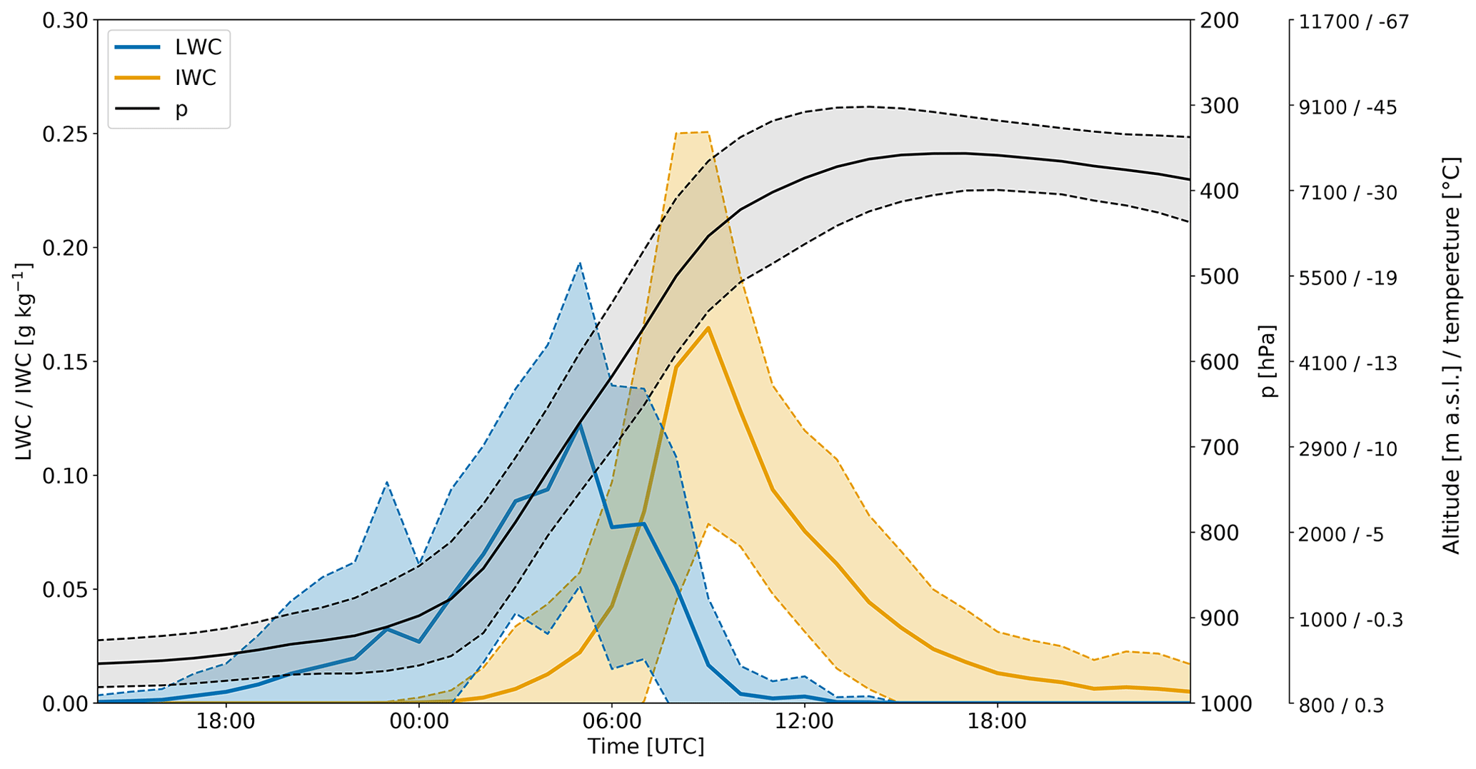
Figure 4Temporal evolution of LWC (blue line; in grams per kilometre) and ice water content (IWC; yellow line, in grams per kilometre) from IFS analyses along the WCB trajectories (black line and grey shading represent the pressure level of the selected trajectories in hectopascals) shown in Fig. 3. Shown are the mean (solid lines) and the standard deviation (dashed lines and shading). The altitudes and temperatures of the pressure levels (second y axis on the right) are taken from the radiosounding at 06:00 UTC.

Figure 5Time series on 28 February 2018 of (a) reflectivity and (b) mean Doppler velocity from WProf (defined positive upwards). (c) Hydrometeor classification (Besic et al., 2018) based on MXPol RHIs towards MHS. Only data with an elevation angle between 5∘ and 45∘ are considered. The isolines represent the proportion of each hydrometeor class normalised by the average number of pixels per time step. The contour interval is 2 %. The yellow contours represent crystals, the blue ones aggregates and the red ones rimed particles. The results are shown only above 2000 m since the lower altitudes are contaminated by ground echoes. The black contour in panels (a), (b) and (c) shows the boundary of the WCB based on the projection of the trajectories in an Eulerian reference frame (see Sect. 2.4). (d) Brightness temperature (Tb) from the radiometer; (e) precipitation rate (PR; Pluvio2 weighing rain gauge) at MHS (yellow) and GWU (black) and temperature at MHS (blue).
In the previous section, we identified SLW associated with large-scale WCB ascents in IFS analyses. In the following, we use remote and in situ observations to corroborate the presence of SLW and to discuss its relevance for the microphyisical processes taking place.
Before the onset of precipitation, a temperature inversion at 1500 m (Fig. 6a at 00:00 UTC) favours the formation of a low-level cloud (Fig. 5a). This temperature inversion is located just above a layer of potential instability with equivalent potential temperature (θe) gradients of about −10 K km−1 between 1250 and 1450 m. Other layers of potential instability are present below 3000 m (with θe-gradients up to −5 K km−1) for all three radiosoundings at 00:00, 06:00 and 09:00 UTC. Above 3000 m, the air is saturated or close to saturation with respect to ice (Fig. 6b at 00:00 UTC). At 06:00 and 09:00 UTC, the air is saturated with respect to ice over almost the entire troposphere. Between 6000 and 9000 m, the relative humidity with respect to ice (RHi) is well above saturation at 00:00, 06:00 and 09:00 UTC. This altitude range corresponds to the outflow of WCB air masses (Fig. 4), which often features cirrus clouds (Madonna et al., 2014). These cirrus in the WCB outflow are likely composed of both ice crystals formed by freezing of liquid droplets in the WCB ascent and ice crystals formed via nucleation directly from the vapour phase in upper tropospheric air masses pushed upwards by the WCB (Wernli et al., 2016). This suggests that the high supersaturation with respect to ice above 6000 m is directly related to the WCB. In this view, the WCB provides favourable conditions for rapid crystal growth, leading to precipitation onset. The profile of wind speed clearly shows a strong jet of 45 m s−1 at 6500 m a.s.l. at 06:00 UTC (Fig. 6c), which coincides with the WCB air masses. The height of this jet and the lower limit of WCB air masses decrease with time, and we observe the jet just below 5000 m at 09:00 UTC.
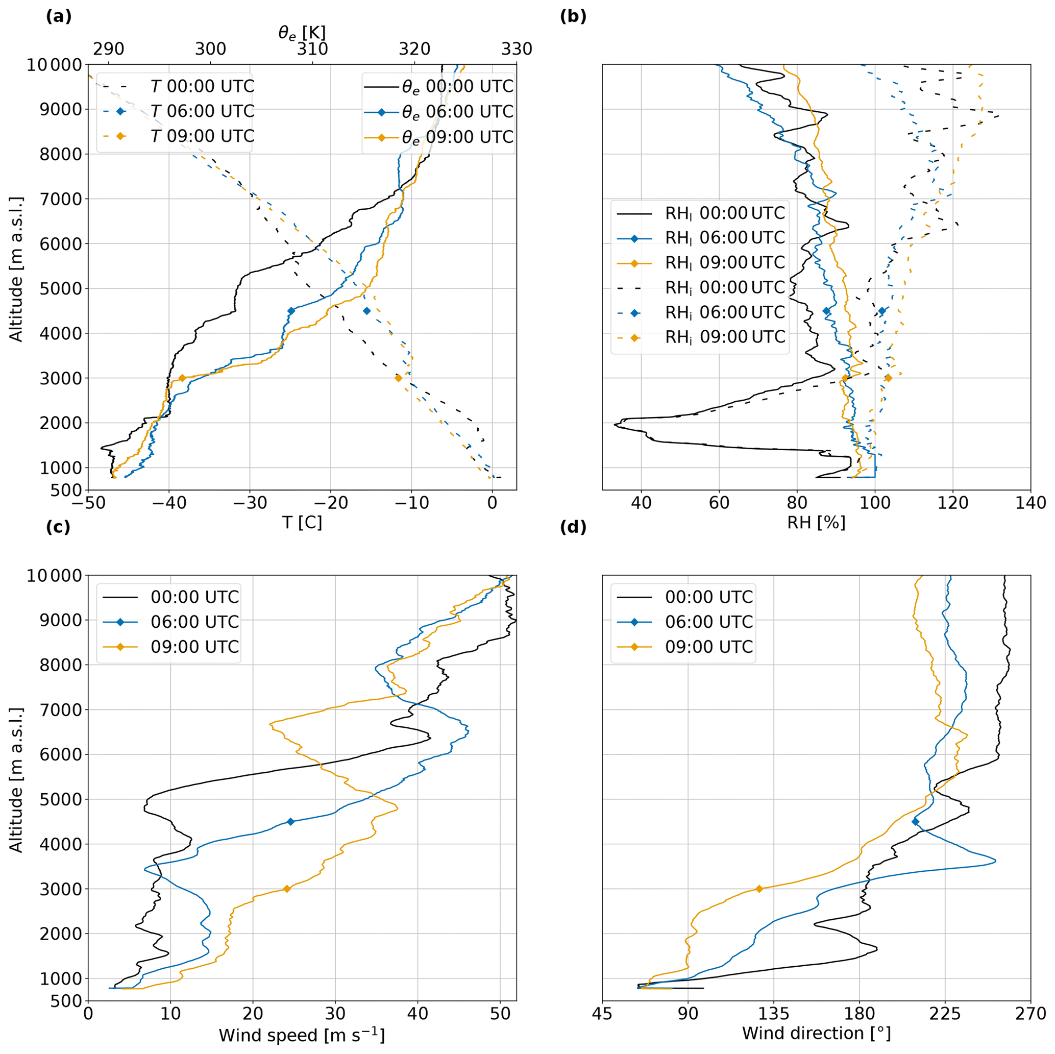
Figure 6Radiosoundings at the DGW station showing (a) temperature (dashed lines) and equivalent potential temperature (solid lines); (b) relative humidity with respect to liquid (RHl; solid lines) and ice (RHi; dashed lines); (c) wind speed; and (d) wind direction at 00:00 UTC (black), 06:00 UTC (blue) and 09:00 UTC (yellow) on 28 February 2018. The diamond symbols for the radiosoundings at 06:00 and 09:00 UTC show the altitude of the lower limit of the WCB (black contour in Fig. 5a, b, c).
In the layer from 4000 to 6000 m a.s.l. at 06:00 UTC an increase in wind speed with height and a rapid change in the wind direction from southerly to south-westerly result in strong vertical wind shear. The vertical wind shear reaches values of 15 in speed and 0.27 ∘ m−1 in direction. Keppas et al. (2018) identified similar values of vertical wind shear, which triggered Kelvin–Helmholtz instabilities. In Sect. 5.3, we illustrate the influence of this vertical wind shear within the WCB ascent region on the observed microphysics.
Figure 5a shows the reflectivity measured by WProf. The nimbostratus cloud approaches between 00:00 and 03:00 UTC. The cloud base is at 3100 m (Fig. 6b), but virgae appear down to 2000 m, where ice crystals sublimate in unsaturated air. Below the temperature inversion at 1400 m the air is close to saturation (Fig. 6a, b at 00:00 UTC), and a low-level cloud can be identified as a layer with reflectivity values below −5 dBZ. At 03:00 UTC surface precipitation starts and lasts until 16:00 UTC (Fig. 5e). A 3D gridding of the WCB trajectory positions (Fig. 5,a, b, black contour) reveals that WCB air parcels continuously ascend above the location of WProf during the entire passage of the nimbostratus cloud. At 19:00 UTC a post-frontal precipitating system sets in and lasts until 00:00 UTC on 1 March. It is not associated with the WCB and is not investigated.
Within the WCB ascent regions, enhanced updraughts are present, in particular around 3000 m a.s.l. between 07:00 and 10:00 UTC (Fig. 5b). These overturning cells at the lower boundary of the WCB (represented by the black contour) are likely Kelvin–Helmholtz instabilities generated by the strong vertical wind shear observed in the radiosoundings (Fig. 6). Except for a moist neutral layer around 4000 m at 06:00 UTC, the profiles at 06:00 and 09:00 have stable lapse rates, which together with a strong wind shear provide favourable conditions for Kelvin–Helmholtz instabilities. A region of enhanced positive Doppler velocity can be observed from 07:30 to 08:00 UTC between 4000 and 6000 m, where the mean Doppler velocity amounts to approximately 2 m s−1, indicating the presence of embedded updraughts in the WCB. Recently, case studies by Keppas et al. (2018), Oertel et al. (2019) and Oertel et al. (2020) identified embedded convection within the large-scale WCB. Oertel et al. (2019) and Oertel et al. (2020) showed that embedded convection leads to a local increase in precipitation intensity, while Oertel et al. (2020) found that it also promotes the formation of graupel particles in the model simulations. Finally, Hogan et al. (2002) observed that embedded convection was collocated with maxima of SLW concentration. In this paper we refer to these upward air motions as embedded updraughts since there is no evidence of convective instability in the radiosoundings (Fig. 6a). While the cause of the updraughts we observe might be different than those mentioned in Hogan et al. (2002), Keppas et al. (2018) and Oertel et al. (2019), the consequence for the precipitation growth processes is consistent with what we observe in this study.
Ahead of the precipitating system the cloud contains mainly crystals (Fig. 5c). Intense precipitation begins around 04:30 UTC, and aggregates dominate during the whole precipitation period. Rimed particles are also present, especially between 06:00 and 08:00 UTC, when the proportion and vertical extent of rimed particles are the largest.
The brightness temperature measured by the radiometer (Fig. 5d) is the primary variable used to estimate the liquid-water path (e.g. Küchler et al., 2017). In this study, we use the brightness temperature as an indicator of the temporal evolution of the total liquid water in the atmospheric column. The maxima of brightness temperature observed when precipitation starts just before 04:00 UTC and the peak at 06:00 UTC corresponding to the local maximum of precipitation rate (Fig. 5e) are probably due to the partial melting of hydrometeors since the temperature at MHS is above 0 ∘C. The multiple peaks after 07:00 UTC (temperature drops below freezing), which co-occur with updraughts, suggest that the updraughts favour the production of SLW in addition to the SLW produced by the large-scale ascent in the WCB. There was unfortunately no CALIPSO (satellite on-board lidar) overpass to ascertain the presence of SLW during the event. There is a local maximum in the precipitation rate just after 06:00 UTC at both MHS and GWU (Fig. 5e), while the absolute maximum is about 12 mm h−1 at 09:40 UTC at MHS and 13 mm h−1 at 14:25 UTC at GWU. Except for the maximum at 14:25 UTC at GWU and the fact that precipitation occurred from 20:00 to 23:59 UTC at MHS but not at GWU, the temporal evolution of precipitation at both locations is very similar. Note that the surface warm front never reached Pyeongchang (only the precipitation associated with it) but moved further to the east. Hence, in contrast to the temperature in the mid-troposphere, which increased by approximately 5 to 10 ∘C (Fig. 6a) during the event, the surface temperature did not increase.
In the previous section we analysed the evolution of the dynamics and microphysics of the nimbostratus and precipitation associated with the warm front. In this section, we analyse succeeding periods that reveal the link between the temporal evolution of the WCB and the microphysics over Pyeongchang. Based on the homogeneity of the dominant microphysical processes, three different periods were selected: we first investigate the period dominated by depositional growth of crystals (Sect. 5.1) and subsequently analyse the effect of embedded updraughts on aggregation and riming (Sect. 5.2). Finally, we consider the impact of vertical wind shear and turbulence on aggregation (Sect. 5.3).
5.1 Vapour deposition: 03:00 to 04:00 UTC
The period from 03:00 to 04:00 UTC is dominated by crystals above 2000 m (Fig. 5c). At this time Pyeongchang is located ahead of the warm front. The vertical profiles of polarimetric variables (Fig. 7) show an increase in ZH of 2 dBZ from 6000 to 2000 m, while ZDR is almost constant from 6000 to 3000 m and then subsequently decreases slightly. This likely indicates the onset of aggregation at 3000 m, below which temperatures are greater than −10 ∘C and hence represent favourable conditions for aggregation (Hobbs et al., 1974). Kdp values are almost zero, suggesting that the number concentration of oblate crystals is low. In summary, this period is characterised by the presence of crystals in limited concentration, which grew by vapour deposition and likely aggregated below 3000 m.

Figure 7Vertical profiles of quantiles of ZH, ZDR, Kdp and SW from MXPol from 03:00 to 04:00 UTC on 28 February 2018. The red line shows the median, while the solid blue lines show the 25th and 75th percentiles and the dotted blue lines the 5th and 95th percentiles. The statistics are based on 11 RHIs towards the MHS site. The data within a horizontal distance of 7 to 20 km from MXPol are selected.
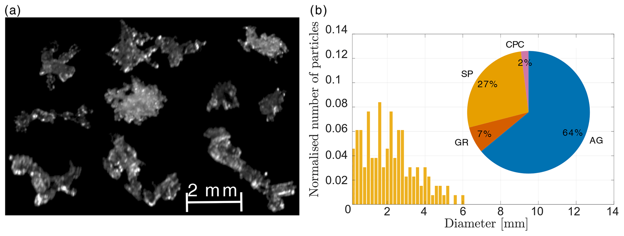
Figure 8(a) Selection of in-focus MASC images. (b) Normalised size distribution and classification of 55 particles observed from 03:00 to 04:00 UTC. SP represents small particles, CC columnar crystals, PC planar crystals, AG aggregates, GR graupel, and CPC a combination of planar and columnar crystals. The size distribution is normalised by the number of particles. The pictures of panel (a) were selected to be representative of the classification. The average temperature was 1.5 ∘C (Fig. 5e).
The selection of snowflake images (Fig. 8b; collected at an average temperature of 1.5 ∘C) mainly shows small aggregates and crystals of about 2 mm in their maximum dimension. They are partly melted (liquid water is less reflective than ice and creates the dark areas on the snowflake pictures), and riming is indicated by the brighter areas. The size distribution shows that most particles are below 5 mm in size, with a median of 2.2 mm. The classification shows that 64 % of the observed hydrometeors are aggregates, while above 2000 m, the MXPol hydrometeor classification shows predominantly ice crystals (Fig. 5c). This supports our previous conclusion that below 3000 m, when the temperature increases and aggregation is more efficient, a large fraction of crystals aggregate. A total of 7 % of particles were identified as graupel (Fig. 8b), which we could confirm by a visual analysis. Again the riming could have taken place below 2000 m, which explains why no rimed particles are present from 03:00 to 04:00 UTC in the MXPol hydrometeor classification of Fig. 5c. Figure 9a shows the distribution of the riming index (0= no riming; 1= graupel; Praz et al., 2017). The mode around 1 corresponds to the graupel particles, while half of the particles had a riming index smaller than 0.4. This shows that except for the few graupel particles, the other hydrometeor classes did not feature significant riming in comparison with other periods of the event.
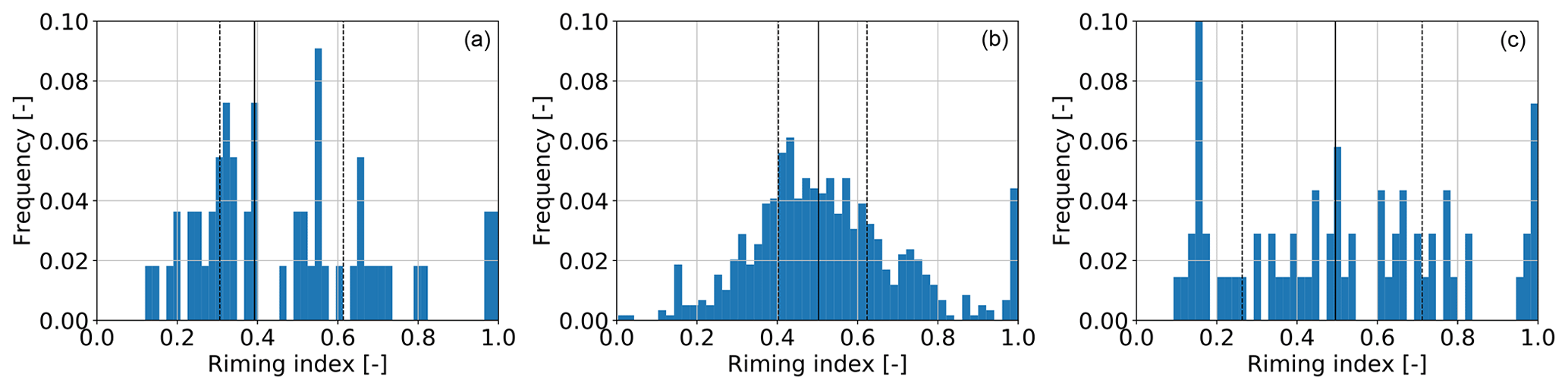
Figure 9Distribution of the riming index for all particles between (a) 03:00 and 04:00 UTC, (b) 06:00 and 08:00 UTC, and (c) 09:00 and 11:00 UTC. The dashed lines show the lower and upper quartiles; the solid line shows the median of the distribution.
5.2 Embedded updraughts, riming and aggregation: 06:00 to 08:00 UTC
The period from 06:00 to 08:00 UTC is characterised by embedded updraughts (Fig. 5b), a layer with strong vertical wind shear at 3800 m (Fig. 6c, d) and significant riming, as seen by MXPol (Fig. 5c). From 6000 to 4800 m the crystals grow by vapour deposition, leading to an increase in both ZH and ZDR (Fig. 10) as particles grow mainly along their longest dimension, which results in larger and more oblate crystals (Schneebeli et al., 2013; Andrić et al., 2013; Grazioli et al., 2015). The median of Kdp increases to only 0.4 , suggesting that the number concentration of oblate particles is small. The temperature in this layer varies from −23 ∘C to −16 ∘C, and the air is slightly above saturation with respect to ice (Fig. 6a, b). This represents favourable conditions for depositional growth of sectored plates (Lohmann et al., 2016; Fig. 8.15), while aggregation is unlikely to dominate within this temperature range according to Hobbs et al. (1974). However, we cannot rule out the formation of early aggregates, which at this stage would be oblate and hence contribute to the increase in ZDR (Moisseev et al., 2015).
At 4800 m we observe a peak and subsequent decrease in ZDR, which marks the end of growth dominated by vapour deposition. We hypothesise that aggregation starts at this altitude. First, snowflakes tend to be less oblate and less dense after aggregation, which explains the decrease in ZDR. Second, aggregation increases the size of snowflakes, and hence ZH continues to increase.
The observed increase in Kdp below the peak in ZDR is a commonly observed but not fully understood feature. Andrić et al. (2013) proposed that secondary ice generation of small oblate crystals could explain the observed enhanced Kdp values. Concentration of secondary ice particles can be much larger than the number of snowflakes they originate from, which would affect Kdp more strongly than ZDR since the former is more sensitive to concentration. Moisseev et al. (2015) suggested that it is the result of the onset of aggregation, producing early aggregates that are relatively oblate. Our hypothesis is that first, the generation of secondary ice by droplet shattering (Mason and Maybank, 1960) and by ice–ice collisions (Vardiman, 1978; Takahashi et al., 1995; Yano and Phillips, 2011) contribute to the increase in Kdp below 5000 m a.s.l. Droplet shattering shows a maximum occurrence at −17 ∘C (Leisner et al., 2014), which corresponds to the altitude where LWC is converted into IWC (Fig. 4 around 5000 m a.s.l.). Secondary ice generation by ice–ice collision is most effective at −15 ∘C (Takahashi, 1993) and may also take place at around 5000 m a.s.l. Second, riming of already-oblate crystals will tend to increase Kdp because in the early stage of riming the cavities in the crystals are filled, increasing the density (and thus the dielectric response) of the hydrometeors without changing their aspect ratio. Third, rime splintering by the Hallett–Mossop process (Hallett and Mossop, 1974) below 2500 m a.s.l. (temperature above −8 ∘C) can contribute to maintain high Kdp values. Finally, Korolev et al. (2020) recently suggested that secondary ice produced by shattering of freezing droplets transported above the melting layer could be lifted to higher levels. This may enhance the concentration of secondary ice in regions of strong updraughts. Note that the higher Kdp values compared to the period 03:00–04:00 UTC are primarily due to the increase in precipitation intensity, but the fact that Kdp increases below the onset of aggregation cannot be explained by precipitation intensity only since aggregation decreases the number concentration and the oblateness of the particles. Riming will initially increase Kdp by first filling cavities and hence increasing the density of particles but will later lead to a decrease in Kdp as the rime mass will smooth the particles' shape. There has to be a mechanism which produces a high number concentration of oblate particles to explain an increase in Kdp in a layer dominated by aggregation and riming, and secondary ice production is a good candidate.
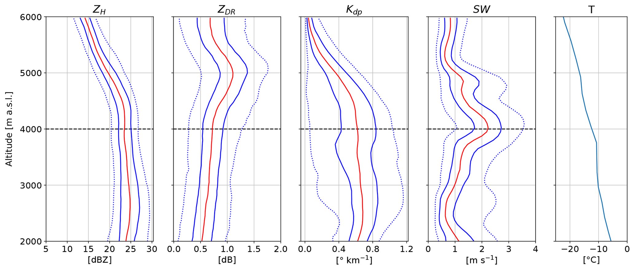
At 3800 m a strong vertical wind shear in the lower part of the WCB (black contour in Fig. 5a, b, c at 06:00 UTC) can be observed in both the radiosoundings (Fig. 6c, d) and the spectral-width profiles (Fig. 10). The jet at 6500 m at 06:00 UTC (Fig. 6c) can be seen as an enhancement of Doppler velocity between 4000 and 6000 m a.s.l., with a maximum of 45 m s−1 at 5000 m in the RHI of Fig. 11. This is in good agreement with the wind speed measured by the radiosonde at 06:00 UTC since the RHI is almost aligned with the wind direction. The vertical wind shear at 3800 m is visible as the Doppler velocity decreases in the lower part of the WCB and reaches a value of 0 m s−1 at 3000 m (combined effect of a decrease in wind speed and change in wind direction from parallel to perpendicular to the radar beam). This vertical wind shear may generate Kelvin–Helmholtz instabilities, which can trigger embedded convection (Hogan et al., 2002). Moreover orography might also play a role in lifting the easterly low-level flow, which directly impinges the Taebaek mountains from the East Sea. These sources of lifting together with the moist neutral layers below 3000 m (Fig. 6a) can lead to the observed strong updraughts (Fig. 5b), which promote aggregation by increasing the probability of collision between particles. The effect of turbulent cells on aggregation has been discussed thoroughly in Houze and Medina (2005), Medina et al. (2005), and Medina and Houze (2015). Houze and Medina (2005) suggested that overturning cells promote both aggregation and riming. First, they can sustain the production of SLW necessary for riming. Second, the turbulence increases the probability of collision between particles. Finally, aggregates are larger targets for the collection of SLW droplets, which again enhances growth by riming. While the cause of the turbulence is different here, the processes described are consistent with our measurements.
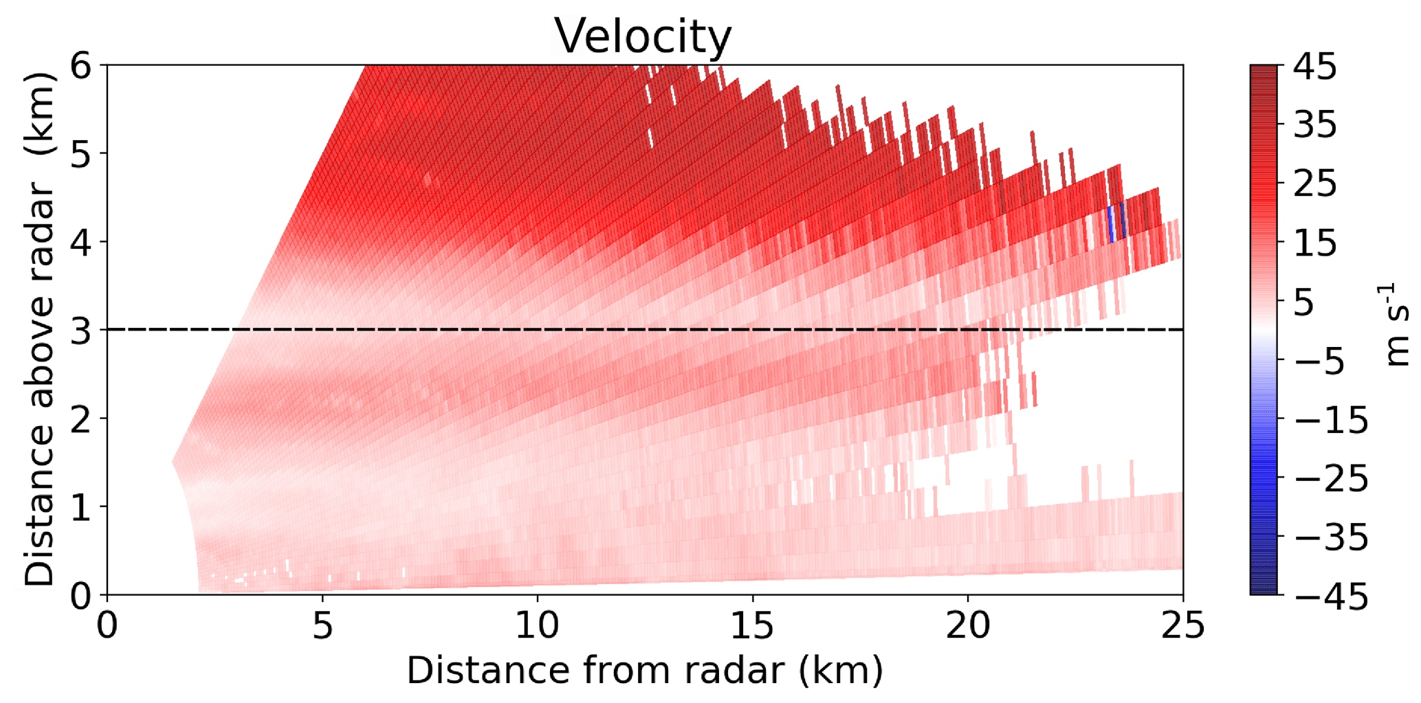
Figure 11RHI of Doppler velocity at 11∘ azimuth at 06:25 UTC from MXPol radar. The dashed black line shows the lower limit of the WCB (black contour in Fig. 5a, b, c). The Python ARM Radar Toolkit (Py-ART; Helmus and Collis, 2016) was used to plot the radar data.
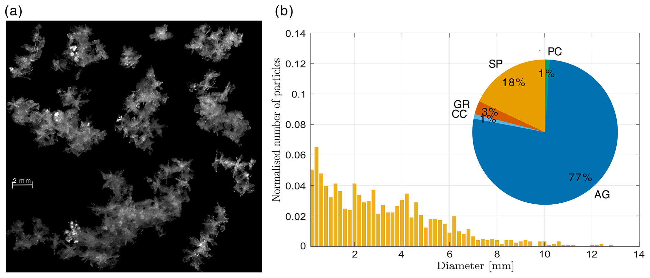
The MASC images (Fig. 12a) show mainly rimed aggregates of about 10 mm in their maximum dimension and two graupel particles. The average temperature of collection was 0.1 ∘C, and hence the particles should not be as melted as during the period 03:00–04:00 UTC. The classification shows a majority of aggregates (77 %). The hydrometeor classification from Besic et al. (2018) classifies rimed aggregates and graupel as rimed particles, whereas the MASC-based classification from Praz et al. (2017) classifies only fully rimed particles as graupel, and the aggregate class also contains rimed aggregates. Therefore a direct comparison of the class aggregates between the two classification methods is difficult. The size distribution is much broader than from 03:00 to 04:00 UTC, with particles reaching 13 mm in their maximum dimension. The median amounts to 2.8 mm as there is still a significant proportion of small particles. The total number of particles is 589, while it was 55 in the previous period, showing that this period features more intense precipitation, which also makes the empirical size distribution more robust. The 75th percentile is 4.7 mm compared to 3.0 mm for the period 03:00 to 04:00 UTC, showing that the particles from 06:00 to 08:00 UTC are significantly larger. These large rimed aggregates can be attributed to the strong updraughts, which enhance the growth by aggregation and riming. Note that while the previous period (Sect. 5.1) featured riming below 2000 m, the precipitation rate was much smaller than from 06:00 to 08:00 UTC (Fig. 5e), and hence this riming did not contribute significantly to the total precipitation accumulation. The important message here is that the flow conditions in the WCB promoted rapid precipitation growth by aggregation and riming above 2000 m and are thus responsible for the large precipitation accumulation between 06:00 and 08:00 UTC. Moreover, most of the particles have higher quartiles of riming index (Fig. 9b) than between 03:00 and 04:00 UTC despite the lower proportion of graupel, which is due to the enhanced aggregation favouring rimed aggregates at the expense of pure graupel. We conclude that this period features the most riming both in absolute mass and in relative terms over all hydrometeor classes.
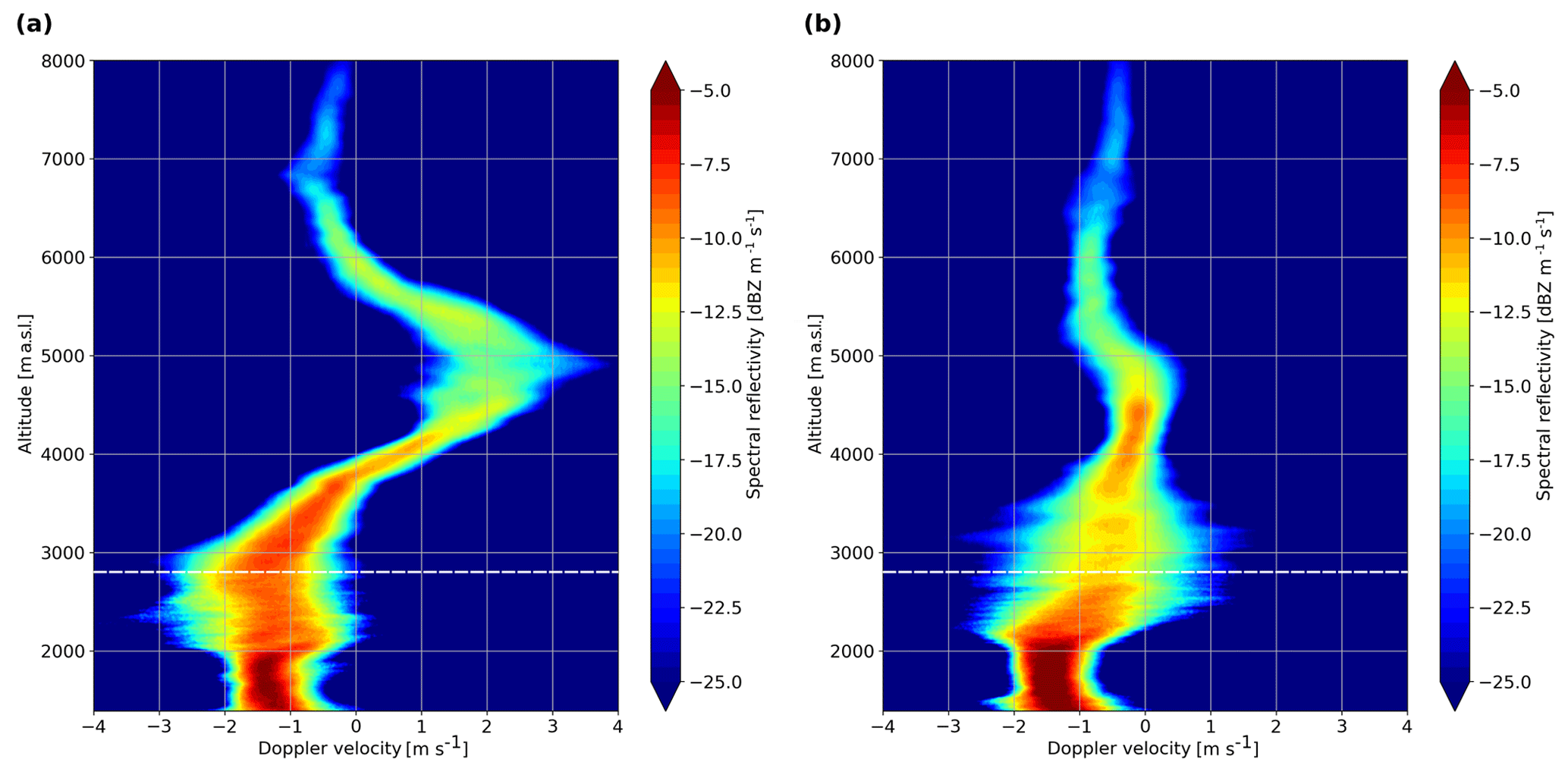
Figure 13Range spectrogram from WProf averaged (a) from 07:42 to 07:47 UTC and (b) from 07:57 to 08:02 UTC. Positive velocity values represent upward motions. The dashed white line shows the lower limit of the WCB (black contour in Fig. 5a, b, c).
Figure 13 shows a range spectrogram from WProf averaged from 07:42 to 07:47 UTC and from 07:57 to 08:02 UTC. The updraught present in Fig. 5b can be seen as a strong shift in the mode of the spectrum from about −0.5 m s−1 at 6000 m to above 2 m s−1 at 5000 m (Fig. 13a). This updraught goes along with strong turbulence, which is visible as an increase in spectral width between 4000 and 6000 m. By 07:57 UTC (Fig. 13b), the increase in spectral reflectivity together with a decrease in Doppler velocity from 4800 to 4000 m suggests that large aggregates likely formed in the turbulent layer and further aggregate during their fall. This is consistent with the onset of aggregation below 5000 m observed in Fig. 10. The enhanced aggregation in the updraughts present from around 07:30 to 08:00 UTC leads to an increase in precipitation rate from 07:55 UTC to the maximum at 09:40 UTC (Fig. 5e). Particles that started falling between 4000 and 5000 m will take 85–105 min to fall to the ground, with an average effective fall speed (absolute fall speed plus updraught) of 0.8 m s−1. This is consistent with the increase in precipitation intensity from 07:55 to 09:40 UTC, and the maximum could correspond to aggregates that formed in the updraught between 07:35 and 07:55 UTC. This hypothesis assumes a certain horizontal homogeneity, supported by the increase in precipitation in both rain gauge measurements at MHS and GWU that are separated by 19 km (Fig. 5e). It would imply that the embedded updraughts are responsible for the period of strongest precipitation, which also features intense riming (Fig. 5c), consistent with the suggestion in Oertel et al. (2019, 2020).
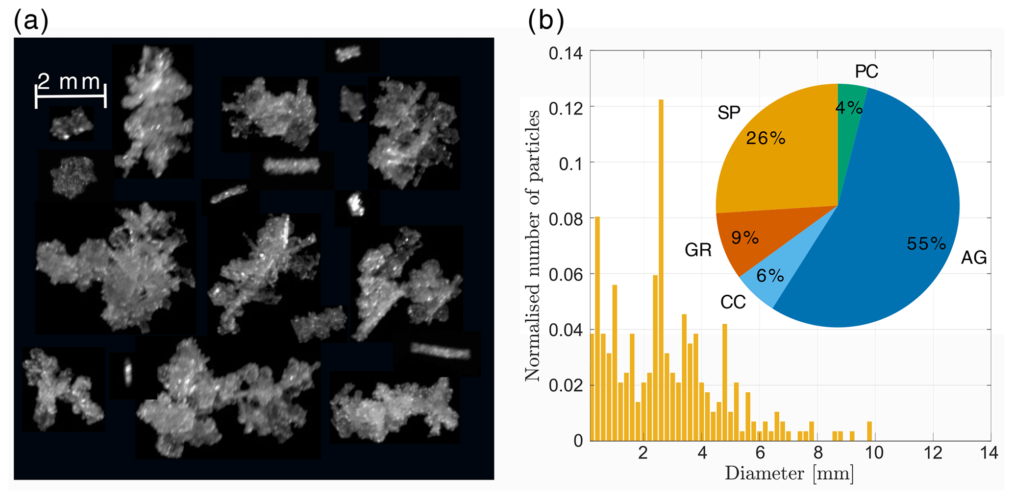
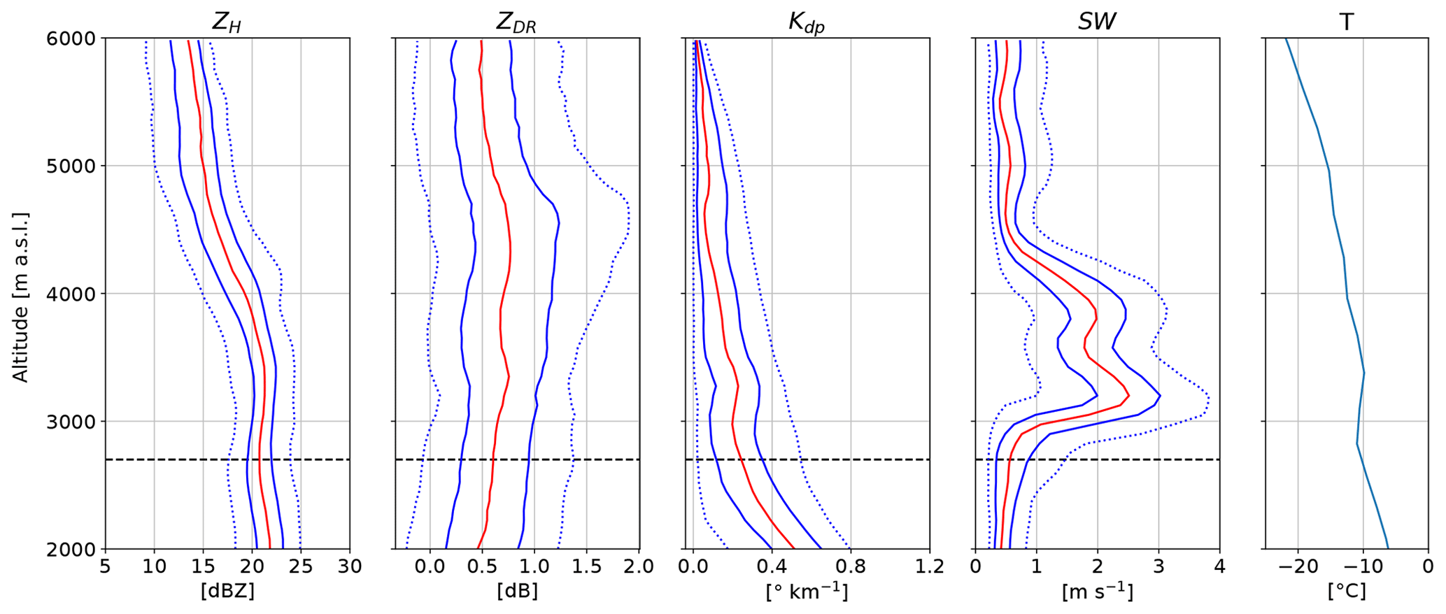
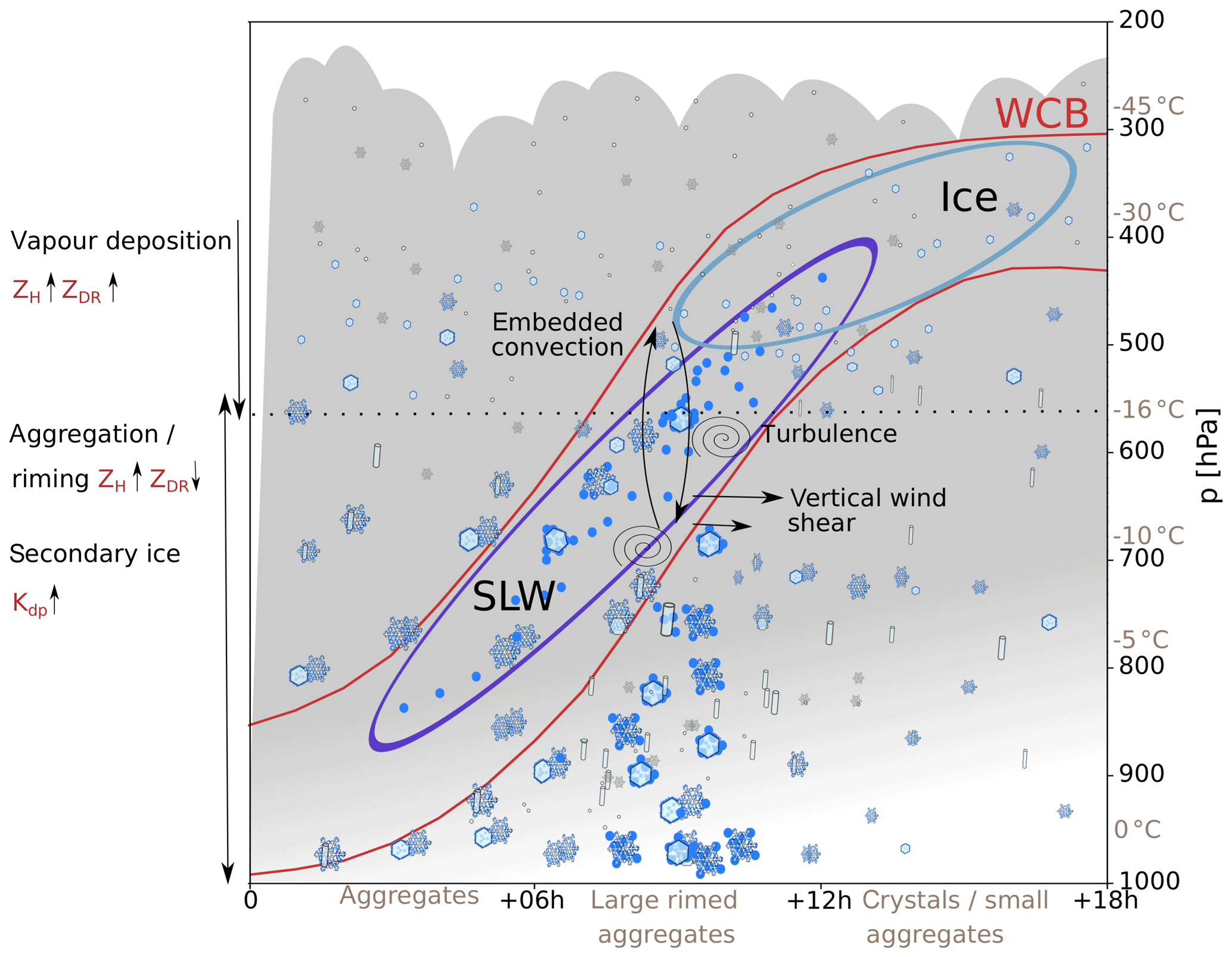
Figure 16Conceptual model in a Lagrangian reference frame (i.e. along the WCB) summarising the key findings. The temperature indications come from the radiosounding at 06:00 UTC (Fig. 6a). The time is indicated as hours from the start of the ascent. The ascent is representative of a strong wintertime WCB.
5.3 Shear-induced turbulence: 09:00 to 11:00 UTC
The period from 09:00 to 11:00 UTC features turbulence and intense precipitation rates (Fig. 5b, e). Due to a malfunction of the MASC, only pictures between 10:08 and 10:50 UTC were collected, leading to only 69 particles during this period (Fig. 14). There are substantially more crystals (10 %) than during the other periods. Figure 14a shows a few small aggregates, columnar and planar crystals, and one graupel particle. The median of the size distribution is 2.7 mm, and the 75th and 95th percentiles are 3.9 mm and 6.6 mm, respectively, indicating that the particles are smaller than in the previous period. Figure 15 shows a less pronounced increase in ZDR compared to the period between 06:00 and 08:00 UTC (Fig. 10), suggesting that the depositional growth rate is smaller than during the previous period. The median of ZDR increases to 0.7 dB around 4200 m, where crystals and aggregates probably dominate. The median of ZH reaches a maximum of 22 dBZ at 2000 m compared to 25 dBZ at 06:00–08:00 UTC (Fig. 10). This is consistent with the size distribution (06:00–08:00 UTC in Fig. 12) that shows more large particles than Fig. 14. Below 4200 m, larger aggregates start to form as temperatures exceed −15 ∘C and ZDR decreases slightly. It is collocated with the increase in spectral width (Fig. 15), reflecting the vertical wind shear below the maximum wind speed (Fig. 6c) at 09:00 UTC. The shear layer was between 4000 and 5000 m in the period from 06:00 to 08:00 UTC, while it is now between 3000 and 4000 m. This vertical wind shear is collocated with the turbulent cells observed in Fig. 5b from 08:00 to 10:00 UTC around 4000 m, which suggests that they originate from Kelvin–Helmholtz instabilities. This is supported by values of the gradient Richardson number (not shown here) of 0.2 where the turbulent cells are present. The decrease in the height of the wind shear is consistent with the decrease in the height of maximum wind speed between 06:00 and 09:00 UTC (Fig. 6c) and explains why the altitude of aggregation enhancement by turbulence decreases with time. This was also observed by Keppas et al. (2018), who attributed this altitude decrease in the maximum wind speed to the passage of the warm front. On the other hand, the altitude of the onset of aggregation could increase with time as the warm front passes because the altitude of the −15 ∘C isotherm (relative maximum aggregation in Hobbs et al., 1974) is higher at 09:00 UTC than at 06:00 UTC. Our interpretation is that the enhancement of aggregation by turbulence dominates the polarimetric signatures in our case: first, because crystals were likely growing as sectored plates and not as dendrites, the latter being more effective to aggregate at −15 ∘C, and second, because the intense aggregation taking place in the shear layer leads to larger aggregates than the early aggregation at −15 ∘C, which makes the former more visible in the polarimetric profiles. The distribution of the riming index (Fig. 9c) is broader than for the other periods due to the higher proportions of crystal-like particles and the presence of graupel and rimed aggregates.
The findings of this case study can be summarised in a conceptual model (Fig. 16). As the WCB rises from the boundary layer, the air saturates, and the liquid-water droplets eventually become supercooled. If the ascent rate is strong enough (which is the case for most WCBs; see Sect. 3), SLW can be produced and persist to the mid-troposphere. Crystals grow by vapour deposition at upper levels of the WCB ascent (see RHi >110 % in Fig. 6b), leading to an increase in ZH and ZDR. During their fall, they experience riming by accretion of supercooled droplets. Moreover, the vertical wind shear (large SW) at the lower boundary of the WCB creates turbulence, which enhances aggregation by increasing the probability of collision between hydrometeors. Furthermore, embedded updraughts in the WCB (as seen by positive vertical Doppler velocities) can additionally lift precipitating particles and increase their time for growth by aggregation. Finally, aggregates are larger targets for collection of SLW, which enhances riming. This leads to large rimed aggregates and local peaks in precipitation intensity. In the layer of growth by aggregation and riming, ZH increases, while ZDR decreases. Additionally, generation of secondary ice by droplet shattering and ice–ice collision leads to an increase in Kdp. In the outflow region of the WCB, crystals, which formed either by nucleation from the vapour phase or freezing of the remaining supercooled droplets, fall and may aggregate without significant riming. While this conceptual model is built upon a single case study, we postulate that the key processes, which are production of SLW and turbulence-enhancing riming and aggregation, can take place in most wintertime mid-latitude cyclones featuring a strong WCB.
This study investigates the snowfall microphysics associated with a WCB during an extreme wintertime precipitation event in South Korea. We combined Doppler dual-polarisation radar measurements, snowflake photographs and radiosonde data with IFS data and trajectories to characterise the detailed precipitation growth mechanisms associated with the large-scale WCB ascent.
The main findings can be summarised as follows:
-
We identified a WCB in IFS analyses as rapidly ascending air masses (approximately 600 hPa in 12 h) in the vicinity of Pyeongchang. A strong jet and enhanced vertical wind shear within the WCB ascent region are clearly visible in radiosonde data and Doppler velocity measurements from MXPol.
-
The IFS analyses show that SLW (up to 0.2 g kg−1) is produced during the rapid ascent in the WCB by condensation of water vapour. In agreement with IFS analyses, multiple peaks in the brightness temperature of the radiometer during the passage of the warm front corroborate the presence of SLW. The timing and presence of SLW are additionally confirmed by the presence of rimed particles observed by the MASC and a hydrometeor classification based on MXPol data.
-
The vertical wind shear promotes aggregation and riming by producing SLW, updraughts and turbulence, which enhance the probability of collision between particles.
-
Three periods could be identified in which the governing microphysical processes are directly influenced by the specific flow conditions in the WCB. In the first period, Pyeongchang is located below the WCB outflow (Fig. 5a). No strong updraughts were present, the precipitation intensity was low and we observed mainly small aggregates and crystals. In the second and third periods, Pyeongchang is located below the WCB ascent. A layer with strong vertical wind shear, whose height decreases with time, generates turbulent cells and updraughts. The precipitation intensity peaks between 7 and 10 mm h−1, and large rimed aggregates are observed.
This study enables the investigation of the impact of a large-scale feature, such as a WCB, on microphysics thanks to the complementarity of atmospheric models, remote-sensing and in situ measurements. It suggests a strong coupling between processes at synoptic and microscales that has to be assessed when evaluating the representation of clouds and precipitation in atmospheric models. While this case study presents a detailed analysis of field measurements, additional investigations with in situ measurements in clouds – characterising the presence of SLW for instance – are needed to further constrain and evaluate the coupling between large-scale dynamical processes and microphysics in models.
Table A1Values of the different variables used in the computation of . Data from IFS analysis and radiosoundings at 09:00 UTC are used. The pressure p used is 610 hPa; temperature T is −13 ∘C.
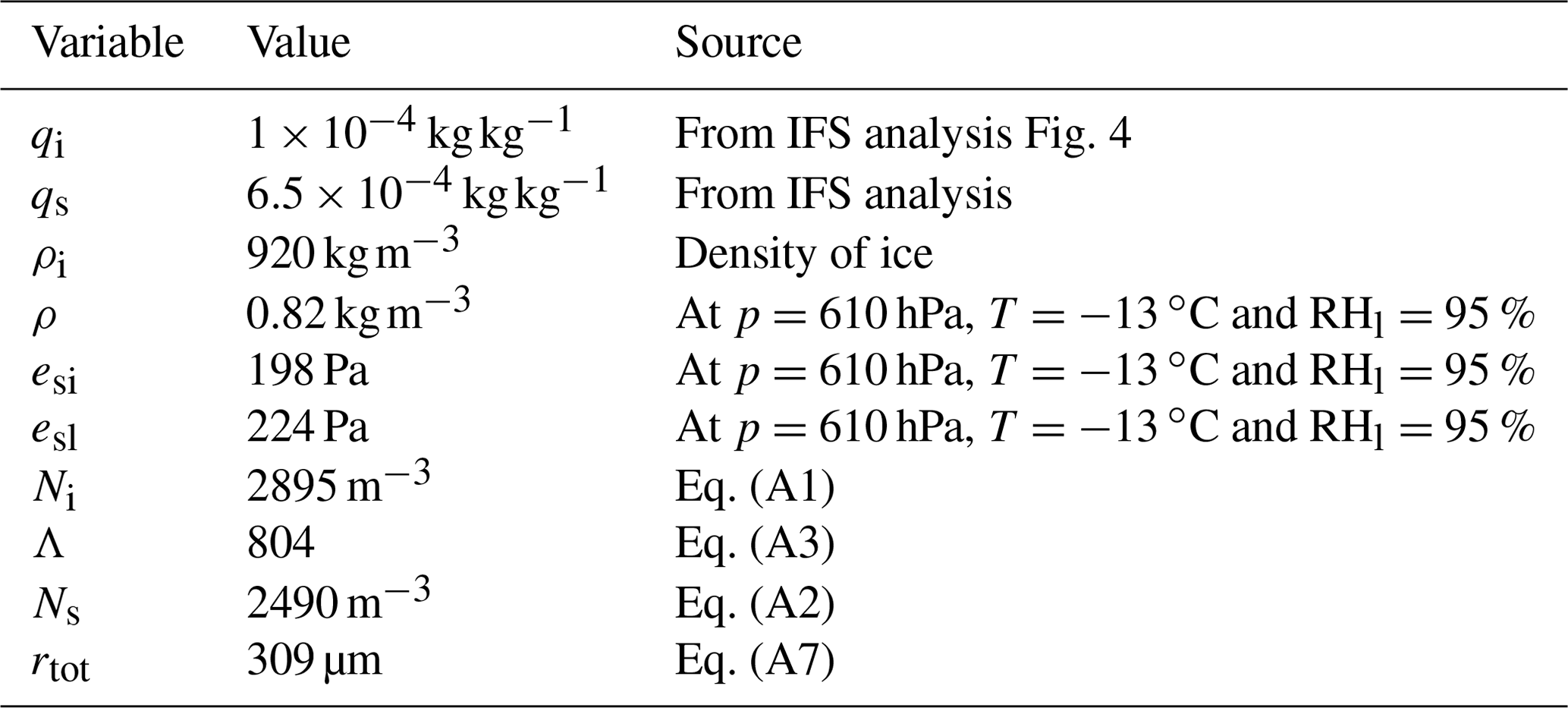
In this appendix we show details on the estimation of the critical vertical velocity needed to form and maintain liquid water in the presence of both ice crystals and snow. Korolev and Mazin (2003) showed that can be expressed as a function of pressure, temperature, number concentration and mean size of ice crystals. We use Fig. 10 in Korolev and Mazin (2003), which gives the relation between and the product of the number concentration of ice particles Ni and the characteristic size of ice particles ri for temperatures between −35 and −5∘C. Since in our case we have both ice and snow particles, we compute Ni and the number concentration of snow particles Ns separately such that the total number concentration is . We also compute the characteristic size of the mixture of ice and snow particles rtot. The expression for Ni is given by Eq. (7.40) of ECMWF (2016):
where esl (esi) is the saturation vapour pressure with respect to liquid (ice). The expression for Ns is given by Eqs. (7.15) to (7.19) in ECMWF (2016). In our case it is simply expressed by
where (Eq. 7.16 and Table 7.1 of ECMWF, 2016), and Λ is given by Eq. 7.18 of ECMWF (2016):
where as=0.069, bs=2 and nbs=0 are given in Tables 7.1 and 7.2 of ECMWF (2016). The expression for ri can be found by stating that the characteristic volume of an ice particle Vi is
where ρ is the air density, ρi the density of ice particles and qi the mixing ratio of ice. Assuming spherical particles, we can express ri with
Since snow particles are spherical in IFS and considered to have the same density as ice, we have ρi=ρs. We define rtot as
Using the values described in Table A1, we find Ntotrtot = 1.7 µm cm−3, which we can use in Fig. 10 of Korolev and Mazin (2003) to read at about −13 ∘C and find 0.1 m s−1.
The trajectories were computed with the Lagrangian analysis tool LAGRANTO (Sprenger and Wernli, 2015). We used functions from the Python libraries Py-ART (Helmus and Collis, 2016) and MetPy (https://doi.org/10.5065/D6WW7G29; May et al., 2008). Other codes and data are available upon request from the corresponding author.
JG and AB designed the experiment. JG operated the instruments and processed and analysed the observational data. AO computed and analysed the WCB trajectories. NJ computed the MASC size distributions. NB computed the radar-based hydrometeor classification. JG, AO, EV and AB interpreted the data. JG, with contributions from all authors, prepared the manuscript.
The authors declare that they have no conflict of interest.
This article is part of the special issue “Winter weather research in complex terrain during ICE-POP 2018 (International Collaborative Experiments for PyeongChang 2018 Olympic and Paralympic winter games) (ACP/AMT/GMD inter-journal SI)”. It is not associated with a conference.
The authors are greatly appreciative to the participants of the World Weather Research Programme Research and Development and Forecast Demonstration Project International Collaborative Experiments for Pyeongchang 2018 Olympic and Paralympic Winter Games (ICE-POP 2018), hosted by the Korea Meteorological Administration. In particular, we are thankful to the High Impact Weather Research Center of the Korea Meteorological Administration for providing us with radiosonde data and giving us access to their facilities at Gangneung–Wonju National University. We would also like to thank Christophe Praz and Jacques Grandjean for their help during the deployment of the instruments. Special thanks go to KwangDeuk Ahn from the Korea Meteorological Administration for his support during the campaign and to Kwonil Kim for his help with some instruments. We are grateful to Andrew Heymsfield and the anonymous reviewer, whose comments helped improve this paper. Finally, we would like to thank Hanna Joos and Heini Wernli from ETH for their constructive comments on the manuscript.
Josué Gehring and Annika Oertel received financial support from the Swiss National Science Foundation (grant nos. 175700/1 and 165941, respectively). Étienne Vignon received financial support from the EPFL-LOSUMEA project. Nikola Besic received financial support from MeteoSwiss through the “Applied research and innovation in radar meteorology” collaboration with EPFL-LTE.
This paper was edited by Timothy Garrett and reviewed by Andrew Heymsfield and one anonymous referee.
Andrić, J., Kumjian, M. R., Zrnić, D. S., Straka, J. M., and Melnikov, V. M.: Polarimetric signatures above the melting layer in winter storms: An observational and modeling study, J. Appl. Meteorol. Clim., 52, 682–700, https://doi.org/10.1175/JAMC-D-12-028.1, 2013. a, b, c
Bader, M. J., Clough, S. A., and Cox, G. P.: Aircraft and dual polarization radar observations of hydrometeors in light stratiform precipitation, Q. J. Roy. Meteor. Soc., 113, 491–515, https://doi.org/10.1002/qj.49711347605, 1987. a, b
Besic, N., Figueras i Ventura, J., Grazioli, J., Gabella, M., Germann, U., and Berne, A.: Hydrometeor classification through statistical clustering of polarimetric radar measurements: a semi-supervised approach, Atmos. Meas. Tech., 9, 4425–4445, https://doi.org/10.5194/amt-9-4425-2016, 2016. a
Besic, N., Gehring, J., Praz, C., Figueras i Ventura, J., Grazioli, J., Gabella, M., Germann, U., and Berne, A.: Unraveling hydrometeor mixtures in polarimetric radar measurements, Atmos. Meas. Tech., 11, 4847–4866, https://doi.org/10.5194/amt-11-4847-2018, 2018. a, b, c
Bringi, V. N. and Chandrasekar, V.: Polarimetric Doppler Weather Radar: Principles and Applications, Cambridge University Press, https://doi.org/10.1017/CBO9780511541094, 2001. a
Browning, K. A.: Organisation of clouds and precipitation in extratropical cyclones, Amer. Meteorol. Soc., Boston, MA, 1990. a, b
Browning, K. A., Hardman, M. E., Harrold, T. W., and Pardoe, C. W.: The structure of rainbands within a mid‐latitude depression, Q. J. Roy. Meteor. Soc., 99, 215–231, https://doi.org/10.1002/qj.49709942002, 1973. a
Carlson, T. N.: Airflow through midlatitude cyclones and the comma cloud pattern, Mon. Weather Rev., 108, 1498–1509, https://doi.org/10.1175/1520-0493(1980)108<1498:ATMCAT>2.0.CO;2, 1980. a
Colle, B. a., Stark, D., and Yuter, S. E.: Surface Microphysical Observations within East Coast Winter Storms on Long Island, New York, Mon. Weather Rev., 142, 3126–3146, https://doi.org/10.1175/MWR-D-14-00035.1, 2014. a
Dacre, H. F., Martínez-Alvarado, O., and Mbengue, C. O.: Linking Atmospheric Rivers and Warm Conveyor Belt Airflows, J. Hydrometeorol., 20, 1183–1196, https://doi.org/10.1175/jhm-d-18-0175.1, 2019. a
Eckhardt, S., Stohl, A., Wernli, H., James, P., Forster, C., and Spichtinger, N.: A 15-year climatology of warm conveyor belts, J. Climate, 17, 218–237, https://doi.org/10.1175/1520-0442(2004)017<0218:AYCOWC>2.0.CO;2, 2004. a, b
ECMWF: IFS Documentation – Cy41r2, Part IV: Physical Processes, available at: https://www.ecmwf.int/sites/default/files/elibrary/2016/16648-part-iv-physical-processes.pdf (last access: 16 April 2020), 2016. a, b, c, d, e
ECMWF: IFS Documentation – Cy43r3: Operational implementation 11 July 2017, Dynamics and numerical procedures, 2017. a, b, c
Forbes, R., Tompkins, A., and Untch, A.: A new prognostic bulk microphysics scheme for the IFS, p. 22, https://doi.org/10.21957/bf6vjvxk, available at: https://www.ecmwf.int/node/9441 (last access: 19 June 2020), 2011. a
Garrett, T. J., Fallgatter, C., Shkurko, K., and Howlett, D.: Fall speed measurement and high-resolution multi-angle photography of hydrometeors in free fall, Atmos. Meas. Tech., 5, 2625–2633, https://doi.org/10.5194/amt-5-2625-2012, 2012. a
Grazioli, J., Lloyd, G., Panziera, L., Hoyle, C. R., Connolly, P. J., Henneberger, J., and Berne, A.: Polarimetric radar and in situ observations of riming and snowfall microphysics during CLACE 2014, Atmos. Chem. Phys., 15, 13787–13802, https://doi.org/10.5194/acp-15-13787-2015, 2015. a, b, c, d
Green, J. S., Ludlam, F. H., and McIlveen, J. F.: Isentropic relative flow analysis and the parcel theory, Q. J. Roy. Meteor. Soc., 92, 210–219, https://doi.org/10.1002/qj.49709239204, 1966. a
Hallett, J. and Mossop, S. C.: Production of secondary ice particles during the riming process, Nature, 249, 26–28, https://doi.org/10.1038/249026a0, 1974. a
Harrold, T.: Mechanisms influencing the distribution of precipitation within baroclinic disturbances, Q. J. Roy. Meteor. Soc., 99, 232–251, 1973. a, b
Hawcroft, M. K., Shaffrey, L. C., Hodges, K. I., and Dacre, H. F.: How much Northern Hemisphere precipitation is associated with extratropical cyclones?, Geophys. Res. Lett., 39, 1–7, https://doi.org/10.1029/2012GL053866, 2012. a
Helmus, J. J. and Collis, S. M.: The Python ARM Radar Toolkit (Py-ART), a Library for Working with Weather Radar Data in the Python Programming Language, Journal of Open Research Software, 4, p. e25,https://doi.org/10.5334/jors.119, 2016. a, b
Heymsfield, A. J.: Precipitation Development in Stratiform Ice Clouds: A Microphysical and Dynamical Study, J. Atmos. Sci., 34, 367–381, https://doi.org/10.1175/1520-0469(1977)034<0367:pdisic>2.0.co;2, 1977. a
Hobbs, P. V., Chang, S., and Locatelli, J. D.: The dimensions and aggregation of ice crystals in natural clouds, J. Geophys. Res., 79, 2199–2206, https://doi.org/10.1029/JC079i015p02199, 1974. a, b, c
Hogan, R. J., Field, P. R., Illingworth, A. J., Cotton, R. J., and Choularton, T. W.: Properties of embedded convection in warm-frontal mixed-phase cloud from aircraft and polarimetric radar, Q. J. Roy. Meteor. Soc., 128, 451–476, https://doi.org/10.1256/003590002321042054, 2002. a, b, c
Houze, R. a. and Medina, S.: Turbulence as a Mechanism for Orographic Precipitation Enhancement, J. Atmos. Sci., 62, 3599–3623, https://doi.org/10.1175/JAS3555.1, 2005. a, b
Joos, H. and Forbes, R. M.: Impact of different IFS microphysics on a warm conveyor belt and the downstream flow evolution, Q. J. Roy. Meteor. Soc., 142, 2727–2739, https://doi.org/10.1002/qj.2863, 2016. a
Joos, H. and Wernli, H.: Influence of microphysical processes on the potential vorticity development in a warm conveyor belt: A case-study with the limited-area model COSMO, Q. J. Roy. Meteor. Soc., 138, 407–418, https://doi.org/10.1002/qj.934, 2012. a, b
Jullien, N., Vignon, É., Reverdin, A., Praz, C., and Berne, A.: Snowfall particle size distributions at Dumont d'Urville station from MASC measurements, in: 27th IUGG Assembly, p. 1, Montréal, 2019. a
Keppas, S. C., Crosier, J., Choularton, T. W., and Bower, K. N.: Microphysical properties and radar polarimetric features within a warm front, Mon. Weather Rev., 146, 2003–2022, https://doi.org/10.1175/MWR-D-18-0056.1, 2018. a, b, c, d, e
Korolev, A., Heckman, I., Wolde, M., Ackerman, A. S., Fridlind, A. M., Ladino, L. A., Lawson, R. P., Milbrandt, J., and Williams, E.: A new look at the environmental conditions favorable to secondary ice production, Atmos. Chem. Phys., 20, 1391–1429, https://doi.org/10.5194/acp-20-1391-2020, 2020. a
Korolev, A. V. and Mazin, I. P.: Supersaturation of water vapor in clouds, J. Atmos. Sci., 60, 2957–2974, https://doi.org/10.1175/1520-0469(2003)060<2957:SOWVIC>2.0.CO;2, 2003. a, b, c
Küchler, N., Kneifel, S., Löhnert, U., Kollias, P., Czekala, H., and Rose, T.: A W-Band Radar–Radiometer System for Accurate and Continuous Monitoring of Clouds and Precipitation, J. Atmos. Ocean. Tech., 34, 2375–2392, https://doi.org/10.1175/JTECH-D-17-0019.1, 2017. a, b
Kumjian, M.: Principles and applications of dual-polarization weather radar. Part III: Artifacts, J. Operat. Meteorol., 1, 265–274, https://doi.org/10.15191/nwajom.2013.0121, 2013. a, b
Kumjian, M. R., Rutledge, S. A., Rasmussen, R. M., Kennedy, P. C., and Dixon, M.: High-resolution polarimetric radar observations of snow-generating cells, J. Appl. Meteorol. Clim., 53, 1636–1658, https://doi.org/10.1175/JAMC-D-13-0312.1, 2014. a
Leisner, T., Pander, T., Handmann, P., and Kiselev, A.: Secondary ice processes upon heterogeneous freezing of cloud droplets, in: 14th Conf. on Cloud Physics and Atmospheric Radiation, Amer. Meteor. Soc., Boston, MA, 2014. a
Lohmann, U., Luond, F., and Mahrt, F.: An Introduction to Clouds, Cambridge Univ. Press, 2016. a
Madonna, E., Wernli, H., Joos, H., and Martius, O.: Warm conveyor belts in the ERA-Interim Dataset (1979–2010). Part I: Climatology and potential vorticity evolution, J. Climate, 27, 3–26, https://doi.org/10.1175/JCLI-D-12-00720.1, 2014. a, b, c, d, e, f
Mason, B. J. and Maybank, J.: The fragmentation and electrification of freezing water drops, Q. J. Roy. Meteor. Soc., 86, 176–185, https://doi.org/10.1175/1520-0469(1975)032<0974:TFAEOF>2.0.CO;2, 1960. a
May, R. M., Arms, S. C., Marsh, P., Bruning, E., and Leeman, J. R.: MetPy: A Python package for meteorological data, https://doi.org/10.5065/D6WW7G29, 2008. a
Medina, S. and Houze, R. A.: Small-Scale Precipitation Elements in Midlatitude Cyclones Crossing the California Sierra Nevada, Mon. Weather Rev., 143, 2842–2870, https://doi.org/10.1175/MWR-D-14-00124.1, 2015. a
Medina, S., Smull, B. F., Houze, R. A., and Steiner, M.: Cross-Barrier Flow during Orographic Precipitation Events: Results from MAP and IMPROVE, J. Atmos. Sci., 62, 3580–3598, https://doi.org/10.1175/jas3554.1, 2005. a
Moisseev, D. N., Lautaportti, S., Tyynela, J., and Lim, S.: Dual-polarization radar signatures in snowstorms: Role of snowflake aggregation, J. Geophys. Res.-Atmos., 120, 12644–12655, https://doi.org/10.1002/2015JD023884, 2015. a, b, c, d
Oertel, A., Boettcher, M., Joos, H., Sprenger, M., Konow, H., Hagen, M., and Wernli, H.: Convective activity in an extratropical cyclone and its warm conveyor belt – a case-study combining observations and a convection-permitting model simulation, Q. J. Roy. Meteor. Soc., 145, 1406–1426, https://doi.org/10.1002/qj.3500, 2019. a, b, c, d
Oertel, A., Boettcher, M., Joos, H., Sprenger, M., and Wernli, H.: Potential vorticity structure of embedded convection in a warm conveyor belt and its relevance for large-scale dynamics, Weather Clim. Dynam., 1, 127–153, https://doi.org/10.5194/wcd-1-127-2020, 2020. a, b, c, d
Pfahl, S., Madonna, E., Boettcher, M., Joos, H., and Wernli, H.: Warm conveyor belts in the ERA-Interim data set (1979–2010). Part II: Moisture origin and relevance for precipitation, J. Climate, 27, 27–40, https://doi.org/10.1175/JCLI-D-13-00223.1, 2014. a, b, c
Praz, C., Roulet, Y.-A., and Berne, A.: Solid hydrometeor classification and riming degree estimation from pictures collected with a Multi-Angle Snowflake Camera, Atmos. Meas. Tech., 10, 1335–1357, https://doi.org/10.5194/amt-10-1335-2017, 2017. a, b, c
Rutz, J. J., James Steenburgh, W., and Martin Ralph, F.: Climatological characteristics of atmospheric rivers and their inland penetration over the western united states, Mon. Weather Rev., 142, 905–921, https://doi.org/10.1175/MWR-D-13-00168.1, 2014. a
Schaer, M., Praz, C., and Berne, A.: Identification of blowing snow particles in images from a Multi-Angle Snowflake Camera, The Cryosphere, 14, 367–384, https://doi.org/10.5194/tc-14-367-2020, 2020. a
Schneebeli, M., Dawes, N., Lehning, M., and Berne, A.: High-resolution vertical profiles of X-band polarimetric radar observables during snowfall in the Swiss Alps, J. Appl. Meteorol. Clim., 52, 378–394, https://doi.org/10.1175/JAMC-D-12-015.1, 2013. a, b, c, d
Schultz, D. M.: Reexamining the cold conveyor belt, Mon. Weather Rev., 129, 2205–2225, https://doi.org/10.1175/1520-0493(2001)129<2205:RTCCB>2.0.CO;2, 2001. a
Sprenger, M. and Wernli, H.: The LAGRANTO Lagrangian analysis tool – version 2.0, Geosci. Model Dev., 8, 2569–2586, https://doi.org/10.5194/gmd-8-2569-2015, 2015. a, b
Takahashi, T.: High ice crystal production in winter cumuli over the Japan Sea, Geophys. Res. Lett., 20, 451–454, https://doi.org/10.1029/93GL00613, 1993. a
Takahashi, T., Yoshihiro Nagao, and Kushiyama, Y.: Possible High Ice Particle Production during Graupel–Graupel Collisions, Am. Meteorol. Soc., 52, 4523–4527, 1995. a
Vardiman, L.: The Generation of Secondary Ice Particles in Clouds by Crystal–Crystal Collision, J. Atmos. Sci., 35, 2168–2180, https://doi.org/10.1175/1520-0469(1978)035<2168:tgosip>2.0.co;2, 1978. a
Wernli, H. and Davies, H. C.: A Lagrangian-based analysis of extratropical cyclones. I: The method and some applications, Q. J. Roy. Meteor. Soc., 123, 467–489, https://doi.org/10.1256/smsqj.53810, 1997. a, b, c
Wernli, H. and Knippertz, P.: WCBs and TMEs and Their Relationship to ARs, in: Atmospheric Rivers, edited by: Ralph, F., Dettinger, M., Rutz, J., and Waliser, D., chap. 3.2, pp. XX, 366, Springer International Publishing, https://doi.org/10.1007/978-3-030-28906-5, 2020. a
Wernli, H. and Schwierz, C.: Surface Cyclones in the ERA-40 Dataset (1958–2001). Part I: Novel Identification Method and Global Climatology, J. Atmos. Sci., 63, 2486–2507, https://doi.org/10.1175/JAS3766.1, 2006. a
Wernli, H., Boettcher, M., Joos, H., Miltenberger, A. K., and Spichtinger, P.: A trajectory-based classification of ERA-Interim ice clouds in the region of the North Atlantic storm track, Geophys. Res. Lett., 43, 6657–6664, https://doi.org/10.1002/2016GL068922, 2016. a
Yano, J.-I. and Phillips, V. T. J.: Ice–Ice Collisions: An Ice Multiplication Process in Atmospheric Clouds, J. Atmos. Sci., 68, 322–333, https://doi.org/10.1175/2010JAS3607.1, 2011. a
- Abstract
- Introduction
- Measurement campaign and data set
- Synoptic overview and WCB
- The evolution of clouds and precipitation over Pyeongchang
- Microphysical analysis of periods of interest
- A conceptual model
- Conclusions
- Appendix A: Estimation of the critical vertical velocity
- Code and data availability
- Author contributions
- Competing interests
- Special issue statement
- Acknowledgements
- Financial support
- Review statement
- References