the Creative Commons Attribution 4.0 License.
the Creative Commons Attribution 4.0 License.
 | 22 Jan 2020
Sources and atmospheric dynamics of organic aerosol in New Delhi, India: insights from receptor modeling
Sahil Bhandari
Shahzad Gani
Kanan Patel
Dongyu S. Wang
Prashant Soni
Zainab Arub
Gazala Habib
Lea Hildebrandt Ruiz
Delhi, India, is the second most populated city in the world and routinely experiences some of the highest particulate matter concentrations of any megacity on the planet, posing acute challenges to public health (World Health Organization, 2018). However, the current understanding of the sources and dynamics of PM pollution in Delhi is limited. Measurements at the Delhi Aerosol Supersite (DAS) provide long-term chemical characterization of ambient submicron aerosol in Delhi, with near-continuous online measurements of aerosol composition. Here we report on source apportionment based on positive matrix factorization (PMF), conducted on 15 months of highly time-resolved speciated submicron non-refractory PM1 (NR-PM1) between January 2017 and March 2018. We report on seasonal variability across four seasons of 2017 and interannual variability using data from the two winters and springs of 2017 and 2018. We show that a modified tracer-based organic component analysis provides an opportunity for a real-time source apportionment approach for organics in Delhi. Phase equilibrium modeling of aerosols using the extended aerosol inorganics model (E-AIM) predicts equilibrium gas-phase concentrations and allows evaluation of the importance of the ventilation coefficient (VC) and temperature in controlling primary and secondary organic aerosol. We also find that primary aerosol dominates severe air pollution episodes, and secondary aerosol dominates seasonal averages.
- Article
(2689 KB) -
Supplement
(3727 KB) - BibTeX
- EndNote


Exposure to fine particulate matter (PM) poses significant health risks, especially in densely populated areas (Pope and Dockery, 2006; Apte et al., 2015). The Indian National Capital Region (Delhi NCR, India) is a rapidly growing urban agglomeration and encompasses the second most populated city in the world, with extremely high winter PM concentrations and frequent severe air pollution. According to a recent estimate, Delhi is the world's most polluted megacity, on track to also become the world's most populated megacity by 2028 (World Health Organization, 2018; United Nations, 2018). However, the current understanding of the sources and dynamics of PM pollution in Delhi is limited (Pant et al., 2016b).
Delhi has a long history of studies focused on the quantity and composition of suspended particulate matter (Mitra and Sharma, 2002). Several studies have found extremely high PM10 concentrations (particulate matter smaller than 10 µm in diameter; PM10∼250–800 µg m−3) and detected tracer compounds for vehicular emissions, biomass burning, and plastic burning. Large domestic use of fossil fuels and biofuels was found to correlate with especially high mass and number concentrations of PM observed in the evening and at night. These studies captured various aspects of air quality patterns including diurnal variation, the weekday–weekend effect, seasonal variation, interannual variation, and correlations of total particle number and mass concentrations with gas phase species such as SO2 and NO2 (Sharma et al., 2003; Mönkkönen et al., 2004, 2005a, b). Other studies have discussed the speciation of mass in smaller particles (Chowdhury et al., 2007; Srivastava et al., 2008; Tiwari et al., 2009). Recent studies such as Pant et al. (2015) have emphasized PM2.5 and consistently report high winter concentrations of particulate chloride and nitrate and high sulfate concentrations across both winter and summer seasons. They attribute chloride to sources such as coal combustion and biomass and waste burning using molecular markers. For example, hopanes such as S and R homohopane isomers are tracers for coal combustion, polycyclic aromatic hydrocarbons (PAHs) such as phenanthrene and benzo[a]anthracene are tracers for coal and biomass burning, and sugar anhydrosaccharides such as levoglucosan and mannosan are tracers for wood or biomass combustion (Pant et al., 2015). They also attribute higher winter concentrations to condensation of semivolatile ammonium nitrate and ammonium chloride during low-temperature conditions, weaker wind speeds, and the shallow atmospheric boundary layer in the winter season (Pant et al., 2015, 2016a). In recent years, detailed source-specific profiles of combustion and non-combustion sources in the southeastern Asian region have been developed as a part of studies such as the Nepal Ambient Monitoring and Source Testing Experiment (NAMaSTE) campaign; for example, to discern between garbage burning and dung burning, tracers such as 1,3,5-trimethylbenzene and coprostanol have been identified (IIT Bombay, 2008; Stockwell et al., 2016; Goetz et al., 2018; Jayarathne et al., 2018).
A recent review of receptor modeling studies with a focus on Delhi shows that most PM-based source apportionment studies have attributed Delhi's pollution to vehicular traffic, fossil fuel combustion, and road dust (Pant and Harrison, 2012). However, the differences in particle size cutoff in different studies and techniques used made it difficult to compare results (Pant and Harrison, 2012). Most receptor modeling studies have principally relied on a small number of daily or multi-day filter-based samples collected over temporally restricted sampling periods, thereby limiting the possible application of factor analysis techniques such as positive matrix factorization (PMF) to quantify source contributions for entire seasons at the site. Further, despite Delhi being a continental site, multiple studies attribute significant portions of finer fractions of PM to a sea-salt origin (Sharma et al., 2014; Sharma and Mandal, 2017). Recent studies have also developed bottom-up emissions inventories for the National Capital Territory (NCT) region encompassing the city of Delhi (Guttikunda and Calori, 2013) and conducted multi-season multiple-site PM2.5 source apportionment using bottom-up approaches (IIT Kanpur, 2016; ARAI and TERI, 2018). In these bottom-up studies, as well as similar studies across South Asia, emissions sources such as transport, industry, dust, household solid fuel use, and biomass and waste burning are shown to contribute substantially to PM2.5 (Conibear et al., 2018; GBD MAPS Working Group, 2018; Guo et al., 2018; Apte and Pant, 2019). Although these studies accounted for primary organic carbon and secondary inorganic species such as sulfate and nitrate, they often provide limited information regarding secondary organics. Comparatively fewer studies have reported on PM1 composition. One such study attributes winter (December) and spring (March) chloride peaks to be of non-sea-salt origin (Jaiprakash et al., 2017). They also focus on PM1 composition and source apportionment in Delhi and use HYSPLIT to point to potential chloride sources northwest of the Indian Institute of Technology (IIT) Delhi, such as the industries of salt and metal processing and thermal power plants. As for organics, previous studies are mostly limited to the quantification of organic carbon, elemental carbon, polycyclic aromatic hydrocarbons, and water-soluble organic compounds (Singh et al., 2011; Pant et al., 2015; Sharma and Mandal, 2017).
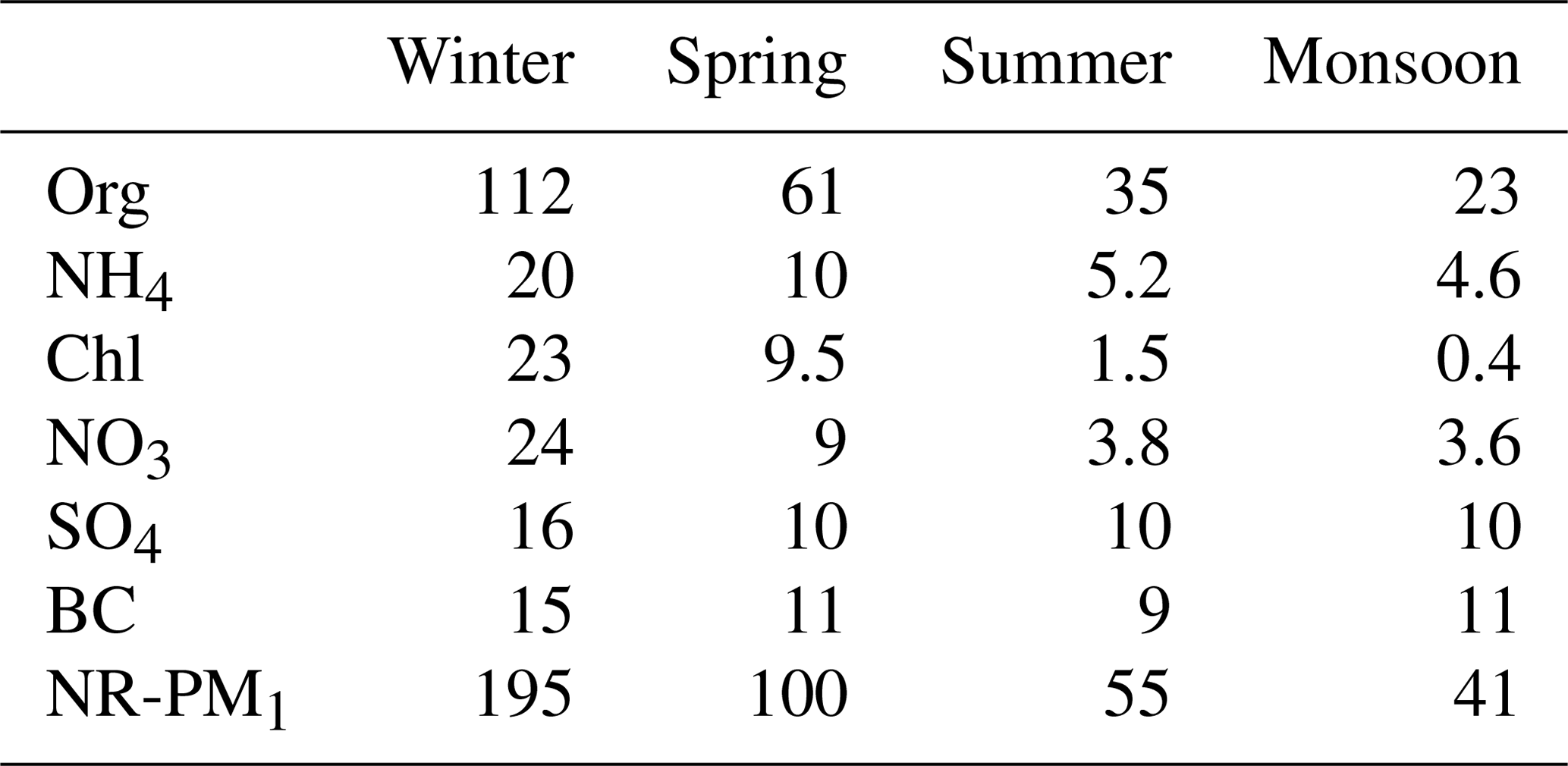
The Delhi Aerosol Supersite (DAS) campaign provides long-term chemical characterization of ambient submicron aerosol in Delhi, with near-continuous online measurements of aerosol composition. Here we report on source apportionment conducted on 15 months of highly time-resolved speciated non-refractory submicron aerosols (NR-PM1), including organics (Org), chloride (Chl), ammonium (NH4), sulfate (SO4), and nitrate (NO3). We use mass spectrometer data from an Aerosol Chemical Speciation Monitor (ACSM) in the PMF receptor model at a time resolution of 5–6 min. This work improves upon the low time resolution of source apportionment utilizing time-integrated filter-based measurements previously employed in Delhi. Over the campaign, organics accounted for 53 % of the submicron mass, followed by inorganics (36%, of which sulfate, nitrate, ammonium, and chloride contributed 13 %, 8 %, 9 %, and 6 %, respectively) and black carbon (BC; 10 %; Gani et al., 2019, Fig. 3). Table 1 provides a summary of key DAS bulk measurements.
Table 1Seasonal summary of PM1 species – the arithmetic mean (AM) for hourly mass concentrations (µg m−3). Adapted from Gani et al. (2019).
In this paper, we focus on organic aerosol and report seasonal variability for four seasons and interannual variability using data from the two winters and springs of 2017 and 2018.
As a part of the DAS campaign, an ACSM (Aerodyne Research, Billerica, MA) was operated at ∼0.1 L min−1 at ∼1 min time resolution in a temperature-controlled laboratory on the top floor of a four-story building at IIT Delhi. Additionally, BC, ultraviolet-absorbing particulate matter (UVPM), and their difference ΔC were measured using a seven-wavelength aethalometer operated at the 1 L min−1 flow rate and 1 min time resolution (Magee Scientific Model AE33, Berkeley, CA) (Drinovec et al., 2015). These instruments were on separate sampling lines, both of which had a PM2.5 cyclone followed by a water trap and a Nafion membrane diffusion dryer (Magee Scientific sample stream dryer, Berkeley, CA). For the ACSM, the scan speed was set at 200 ms amu−1 (amu – atomic mass unit) and pause setting at 125 for a sampling time of 64 s. The ACSM measured mass from the mass-to-charge ratio (m∕z) m∕z 10 to m∕z 140. However, all analysis was restricted to 120 due to smaller mass and large uncertainties associated with data collected at the higher m∕z values (Ng et al., 2011b). All essential calibrations such as flow rate calibration, ionizer tuning, quadrupole resolution adjustment, adjustment of multiplier voltage, m∕z calibration, calibrations for measuring the response factor of nitrate, and relative ionization efficiencies of ammonium and sulfate were performed as recommended. Based on identified issues in the usual jump-mode ionization efficiency calibrations, additional single-scan-mode calibrations for estimating ionization efficiencies were also conducted. For data processing, air beam corrections and the default relative ion transmission corrections were applied. Full details on the sampling site, instrument setup, operating procedures, and calibrations are described in a separate publication (Gani et al., 2019).
2.1 Study design
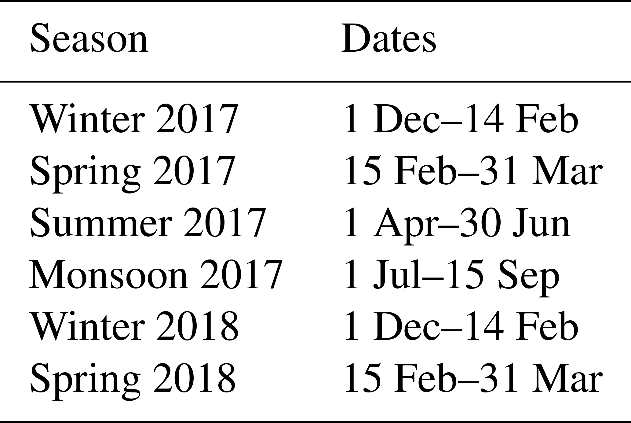
We collected the data used in this paper from January 2017 to March 2018. We conducted separate PMF analysis for each season, with our data categorized into six seasons over these 15 months, as defined by the Indian National Science Academy (2018) (Table 2). We used the dataset obtained by averaging every five consecutive measurements for the seasonal PMF runs. Autumn (mid-September to November) is not included in our core analysis due to the unavailability of ACSM data for that period.
PMF2 has been identified as an appropriate receptor modeling technique that can be deployed for quantifying source contributions for air quality management (Belis et al., 2015). Since the ACSM measures mass spectra at every time point, we obtained two-dimensional matrices of time points (rows) and mass spectral contributions (columns). We deployed the PMF2 program to resolve factors from the 2-D matrices (Paatero and Tapper, 1994). The Igor PMF evaluation tool (PET) was used to conduct PMF2 analysis on this dataset and interpret its results (Ulbrich et al., 2009). Further details on the statistical basis of this method are available elsewhere (Ulbrich et al., 2009; Zhang et al., 2011, and references therein). Briefly, PMF is a bilinear unmixing model that performs deconvolution of mass spectra (MS) into the summation of products of positively constrained mass spectral profiles and their corresponding time series under the assumption that the mass spectral profiles remain constant in time. The iterative PMF technique does not make any assumptions for source or time profiles. In the process, the model minimizes the weighted least-squares error (sum of squares of model error normalized to measurement error), or the summation of squares of scaled residuals of the fit at each data point.
We used two alternative approaches for conducting PMF. In one approach, only organic spectral data at a specific set of m∕z values between m∕z 12 and m∕z 120 were selected. This approach is the most commonly used approach, and the reasons for the selection of the specific set of m∕z values have been described previously (Zhang et al., 2005). In this approach, the concentrations of inorganic species measured by the ACSM were used only as external tracers for interpreting organic PMF factors. However, this technique provides limited information on the relationship between organic and inorganic species (Sun et al., 2012). We pursued a second approach in which we conducted PMF analysis for organic plus inorganic MS. The inorganic m∕z values selected represent the underived m∕z values for each species such that spectral contributions at other m∕z values can be explained completely by data at these m∕z values (Sun et al., 2012; Jimenez group, 2018). Thus, we conducted 12 PMF runs in total (six seasons: organic only and organic–inorganic combined). We refer to the organic MS-based PMF analysis results as “organic-only PMF” and combined organic–inorganic MS-based PMF analysis results as “combined organic–inorganic PMF” results in the paper.
Within the PET, we removed spikes (Zhang et al., 2005) from the dataset, down-weighted mass contribution data at selected weak (signal-to-noise ratio – SNR; SNR < 2) m∕z values by a factor of 2, and removed mass contribution data at bad m∕z values with SNR < 0.2. Further, we used the default fragmentation table, and as a result, higher weight was given to mass spectral contribution at m∕z 44, with which data at m∕z values 16–18 are proportionally related. Accordingly, we down-weighted contributions at these m∕z values by a factor of 2. We readjusted the results from PMF analysis to account for underestimation of factor mass based on the selected m∕z values only. To account for particle losses, we applied transmission and collection efficiencies after conducting PMF analysis (Gani et al., 2019).
2.2 Factor selection
We conducted PMF runs for one to six factors and explored the solution space using the tools FPEAK and SEED. We selected an initial number of p factors based on uncentered correlation coefficients with the factors at the selection p−1. Other criteria employed to select the number of factors include improvement in the solution's ability to explain residual structure with the addition of a factor and ensuring that the 25–75th percentiles of scaled residuals for all m∕z values are between ±3. Changing the SEED value initializes the PMF algorithm with different pseudorandom starts. Changing the FPEAK value allows exploring rotations of solutions of a given number of factors. Primarily, we gauged the effect of the changing FPEAK and SEED using changes in the fraction of variance explained by different factors, correlations of factors' MS with a reference MS, and correlations of factors' time series with the time series of external tracers. Differences between plausible factor solutions in the FPEAK–SEED 2-D space are also representative of the uncertainty of the final selected solution for each scenario in Table 2 (Ulbrich et al., 2009). We observed unreasonable MS, weak time series correlations, or rotational ambiguity on changing FPEAK and/or SEED from the default selection of FPEAK = 0 and SEED = 0. We, therefore, used these default parameter values in our core analysis. Details on factor selection for each PMF run can be found in the Supplement (Sect. S1). We use as reference mass spectra the average mass spectral profiles developed by Ng et al. (2011a) and cooking organic aerosol (COA) and coal combustion organic aerosol (CCOA) profiles in the AMS spectral databases (Ulbrich et al., 2017, 2018), and the one with the highest correlation with the mass spectrum of the PMF-generated factor (generally, Pearson R≥0.9) is used for naming the obtained factor (Ng et al., 2011a). This comparison enables the separation of factors based on their sources, since MS of different factors are characterized by different spectral signature peaks (Zhang et al., 2011). For example, hydrocarbon-like organic aerosol (HOA) is a proxy for fresh traffic and combustion emissions and shows prominent peaks at m∕z values 55 and 57 and a higher fractional organic signal at m∕z 43 than m∕z 44. In this study, carbon monoxide (CO) was not measured. When available, we used CO measured about 11 km (∼7 miles) from our site at a fixed monitoring location, R.K. Puram, maintained by the Central Pollution Control Board (CPCB), government of India, as an external traffic and combustion tracer. Further, we also utilized the co-located aethalometer measurements of BC (880 nm) as a traffic tracer. For biomass burning, we used two tracers: (i) ΔC, defined as the difference between UVPM (370 nm) and BC detected by the aethalometer (Wang et al., 2011; Olson et al., 2015; Tian et al., 2019), and (ii) the biomass-burning component of black carbon, BCBB, estimated using the model of Sandradewi et al. (2008).
In this paper, we focus on the components of organic aerosol obtained using organic-only PMF and combined organic–inorganic PMF. We report average seasonal concentrations of organic-only PMF factors in Table 3 and the organic component of the organic–inorganic combined PMF factors in Table 4. Our results show that the mass spectral profiles of organic-only PMF factors are consistent with reference profiles. In five of the six seasonal organic-only PMF runs, we obtained only two factors – a mixed hydrocarbon-like organic aerosol (HOA) and biomass-burning organic aerosol (BBOA) factor, hereafter referred to as primary organic aerosol (POA), and an oxygenated organic aerosol (OOA) factor. PMF separated HOA and BBOA factors only in spring 2018, and POA MS for this season were calculated by adding these two factors, weighted by their respective time series contributions. Combined organic–inorganic PMF runs further separated the OOA factor but not the POA factor. Advanced factor analysis including the multilinear engine (ME-2) algorithm will be explored in a forthcoming publication to separate the POA factor. Source apportionment conducted in this work was limited to separating primary and secondary OA in all seasons (and, further, primary into BBOA and HOA in spring 2018). Further separation of the factors may be possible with high-resolution data combined with application of factor constraints (Aiken et al., 2009; Elser et al., 2016; Al-Naiema et al., 2018) and source-specific measurements such as metals and metal ions for combustion or biomass-burning emissions (Jaiprakash et al., 2017) or α-methylglyceric acid for biogenic secondary OA (Srivastava et al., 2019).
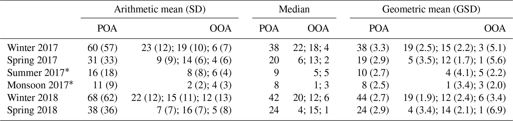
Table 3Organic-only PMF factor concentrations (µg m−3) split into POA and OOA.

* For spring 2018, we were able to separate POA further into HOA and BBOA factors.
Table 4Organic component of the organic–inorganic combined PMF factor concentrations (µg m−3) split into POA and OOA. We were able to separate OOA into AN-OOA, AS-OOA, and AC-OOA.
* For summer and monsoon, OOA was separated only into AN-OOA and AS-OOA, as there was no AC-OOA factor.
Figure 1a presents the mean of the seasonal organic-only PMF POA MS averaged over the entire campaign and the reference profile for HOA. The behavior of this POA factor is in line with the reference HOA factor (see also Figs. S1a–f and S2a–g in the Supplement; R>0.9), as suggested by the dominance of hydrocarbon signatures in the spectrum in the series and (Ng et al., 2010). At the same time, the fractional contributions of the POA factor at m∕z values 29, 60, 73, and 115 are higher compared to the reference HOA factor. These m∕z values have higher contributions from biomass-burning emissions than traffic-related and other combustion emissions (He et al., 2010; Crippa et al., 2014; Bertrand et al., 2017) – comparison with the reference BBOA profile in Fig. S3 points to the influence of biomass burning on the primary organic aerosol factor. As expected, POA tracers, CO and BC, correlate more strongly with the POA factor than with the OOA factor (Fig. S4a–f).
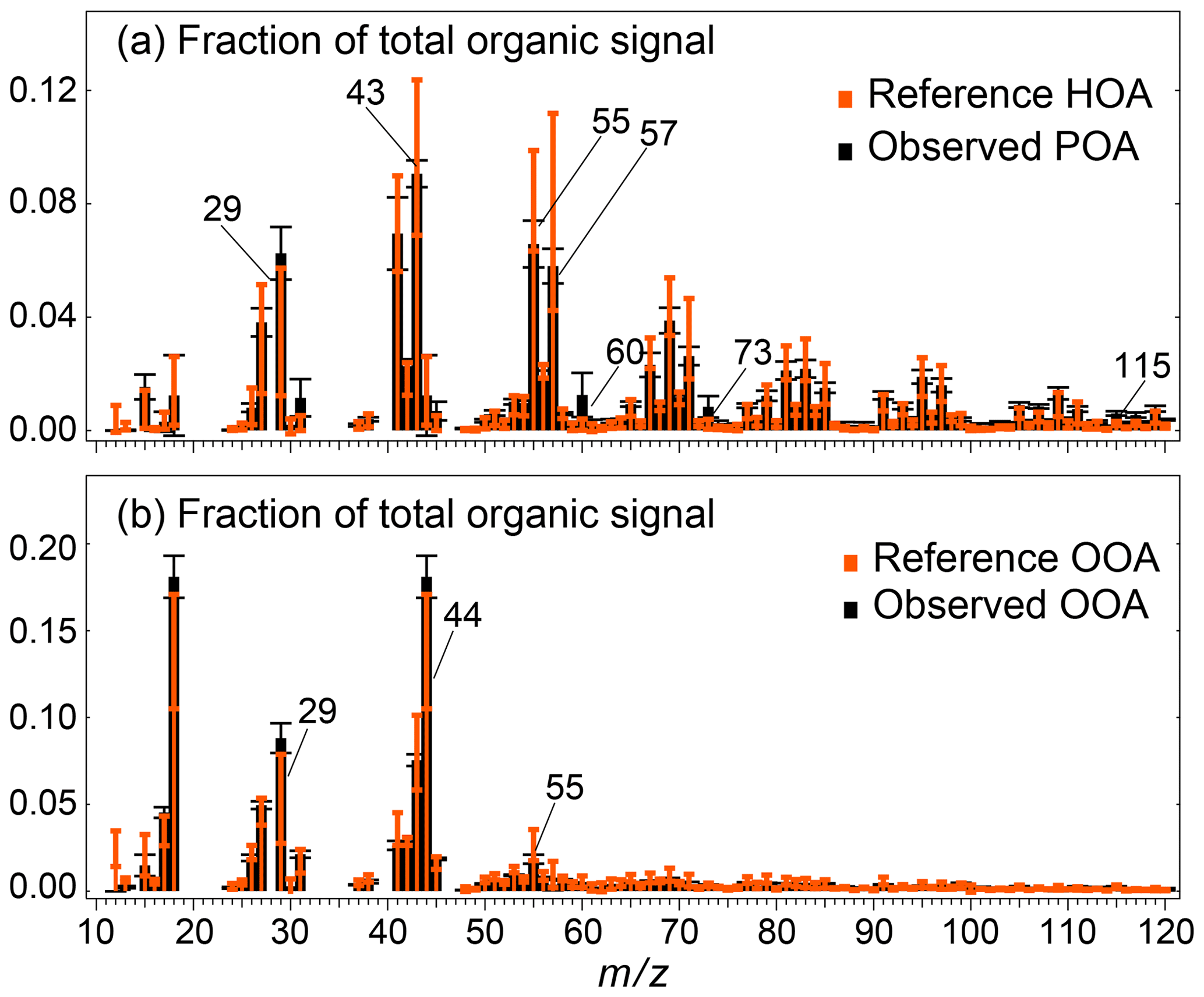
Figure 1(a) The average mass spectrum of organic-only PMF primary organic aerosol (POA) factor shows influence of both hydrocarbon-like organic aerosols (HOA) and biomass-burning organic aerosols (BBOA). (b) The average mass spectrum of organic-only PMF oxygenated organic aerosol (OOA) factor is similar to the reference OOA factor. The whiskers in the graphs represent ±1 SD from the mean spectra.
Figure 1b presents the mean of the seasonal organic-only PMF OOA MS averaged over the entire campaign and the reference profile for OOA. OOA is principally associated with secondary organic aerosol (SOA; Zhang et al., 2011). Mass spectra of the OOA factors in organic-only PMF correlate strongly with the reference OOA factor (R>0.95; Figs. S1a–f and S5a–f). Time series of the OOA factors correlate stronger with secondary inorganic species, such as nitrate and sulfate, compared to their correlations with the POA factor time series (Fig. S4a–f). Figure 2 shows the time series of the organic-only POA and OOA factors for the measurement period. The interplay of sources, meteorology, and photochemistry results in a sharp variation in PMF factor concentrations across seasons. While POA and OOA concentrations are similar in the colder months, OOA is the more abundant component in the warmer months.

Figure 2The 12 h averaged concentration time series (TS) of organic-only PMF oxygenated organic aerosol (OOA) factor and primary organic aerosol (POA) factor (µg m−3). Factor concentrations show strong seasonal variations.
The combined organic–inorganic PMF analysis yielded three or four factors. One factor is predominantly composed of primary organics (accounting for 80 %–95 % of the total factor mass) – we refer to the organic fraction of that factor as POA. An additional two or three factors emerge as a combination of inorganics and oxygenated organics – namely, ammonium sulfate (AS) mixed with OOA (ASOOA), ammonium nitrate (AN) mixed with OOA (ANOOA), and ammonium chloride (AC) mixed with OOA (ACOOA). The time series correlations of the organic–inorganic combined PMF factors with external tracers are shown in Fig. S6a–f. We refer to the organic mass in these mixed factors as AS-OOA, AN-OOA, and AC-OOA, respectively. This organic mass accounts for 19 %–59 % (average 41 %), 21 %–56 % (average 45 %), and 17 %–23 % (average 20 %) of the total mass of these mixed factors, respectively. The mass spectrum of the POA from organic–inorganic combined PMF analysis correlates most strongly with the reference HOA and/or BBOA (R>0.9). AS-OOA and AN-OOA correlate most strongly with the reference low-volatility oxygenated organic aerosol (LVOOA) profile (R>0.95; Fig. S7a–f). It is therefore not surprising, as shown in Fig. S8a–c, that the behavior of POA and OOA in combined organic–inorganic PMF is very similar to that of organic-only POA and OOA, respectively (POA: slope ∼ 1.08, intercept ∼ 1.6, R2∼0.96; OOA: slope ∼ 0.88, intercept ∼ −0.4, R2 ∼ 0.88). Based on the slope of the time series correlations, the combined organic–inorganic PMF estimates ∼8 % more POA and about 12 % less OOA than organic-only PMF, with higher disagreement in warmer months. These differences may be due to a relatively higher m∕z 44 fraction in the POA from combined organic–inorganic PMF analysis than the POA from organic-only PMF analysis (Figs. S9–S14a). Overall, the MS and time series obtained by combining AS-OOA, AN-OOA, and AC-OOA are very similar to the organic-only PMF OOA MS and time series. The mass spectra and time series of the POA and OOA components obtained using combined organic–inorganic PMF factors and organic-only factors are consistently strongly correlated in each season, as shown in Figs. S9–S14a–c.
In Sect. 3.1, we discuss the mass spectral profiles and diurnal time series patterns of POA across seasons. In Sect. 3.2, we discuss the mass spectral profiles and diurnal time series patterns of oxygenated organic aerosol from the seasonal organic-only PMF analysis as well as the combined organic–inorganic PMF analysis. In Sect. 3.3, we contrast the importance of primary versus secondary organic aerosol. We also compare the full PMF results with the tracer-based organic component results. In Sect. 3.4, we investigate interannual variability between the winters and springs of 2017 and 2018 and shed light on the association of PMF factor concentrations with the ventilation-related variables – wind speed, the planetary boundary layer height (PBLH), and the ventilation coefficient (VC = PBLH × wind speed).
3.1 Primary organic aerosol (POA)
The analysis in this section focuses on PMF factors from the organic-only PMF analysis; as suggested by the mass spectral and time series correlations, the behavior of POA in combined organic–inorganic PMF is very similar to the organic-only POA in each season (Figs. S9–S14a–c) and is therefore not discussed here. The factors representing primary organic aerosol have consistently high correlations with hydrocarbon-like organic aerosol and show a varying influence of biomass-burning organic aerosol (Fig. S1a–f). To assess the seasonal variability in this biomass-burning influence on the mass spectra, Fig. S2a–g compares the mass spectra of the POA factors with reference HOA and BBOA profiles. The mixed POA profiles observed in Delhi have fragments at m∕z values 60 and 73, tracers of biomass burning several times the HOA reference profile average and within 15 % of the reference BBOA profile average in winter 2017 and 2018 (Fig. S2a and e). Even in the other three seasons with a mixed POA factor, m∕z 60 and 73 have contributions higher than the reference HOA profile average by more than a standard deviation (Fig. S2b–d). This behavior points to the mixing of biomass burning in the POA factor. In spring 2018, the separated HOA and BBOA are in line with their respective reference profiles (Fig. S2f and g). The mixing of HOA and BBOA factors in PMF has been observed in previous studies as well (Aiken et al., 2009; Elser et al., 2016; Al-Naiema et al., 2018). The deployment of other factorization techniques including the ME-2 algorithm for constraining the presence of POA sources such as cooking and biomass burning is the subject of ongoing work and a forthcoming publication.
The organic-only PMF-based POA diurnal time series patterns exhibit high diurnal, interseasonal, and interannual variability between the winters and springs of 2017 and 2018 and are influenced by episodic pollution events (Table 3; Fig. 3). Peaks in the POA diurnal pattern occur early in the morning and late at night, corresponding to periods of higher traffic. Winter peak POA diurnal concentrations are ∼2 times the diurnal peak in spring, ∼3–5 times the diurnal peak in summer, and ∼6–7 times the diurnal peak in the monsoon season. Additionally, winter peak POA diurnal concentrations are ∼8–10 times winter diurnal minima, and this peak-to-minimum ratio dampens in warmer months – decreasing to ∼5–6 times in summer. We observed larger nighttime (18:00–22:00 LT – local time) and smaller daytime (06:00–09:00 LT) POA peaks. As the sun sets, radiative cooling of the ground surface flips the ambient temperature profile in the surface layer, with ambient temperature increasing with altitude. This inversion layer is thermally stable and traps pollutants at night. As the sun rises, radiative heating warms up the ground surface and the ambient temperature profile returns to a decreasing trend with altitude, which is thermally unstable. Thus, the nighttime and daytime periods encounter similar thermal transition phases, albeit in opposite directions (Figs. 3 and S15; Seinfeld and Pandis, 2016). However, the nighttime period is accompanied by minimal photochemical conversion of POA to SOA in the evening, confirmed by the lower OOA, AN-OOA, and AS-OOA concentrations in the evening (Sect. 3.2). These dynamics could explain the larger nighttime and the smaller daytime POA peaks. Despite a decreasing PBLH and ventilation coefficient at night (21:00–03:00 LT; Fig. S15), POA concentrations are decreasing at night (Fig. 3), likely a consequence of decreasing emissions at night and into the early morning of the next day.
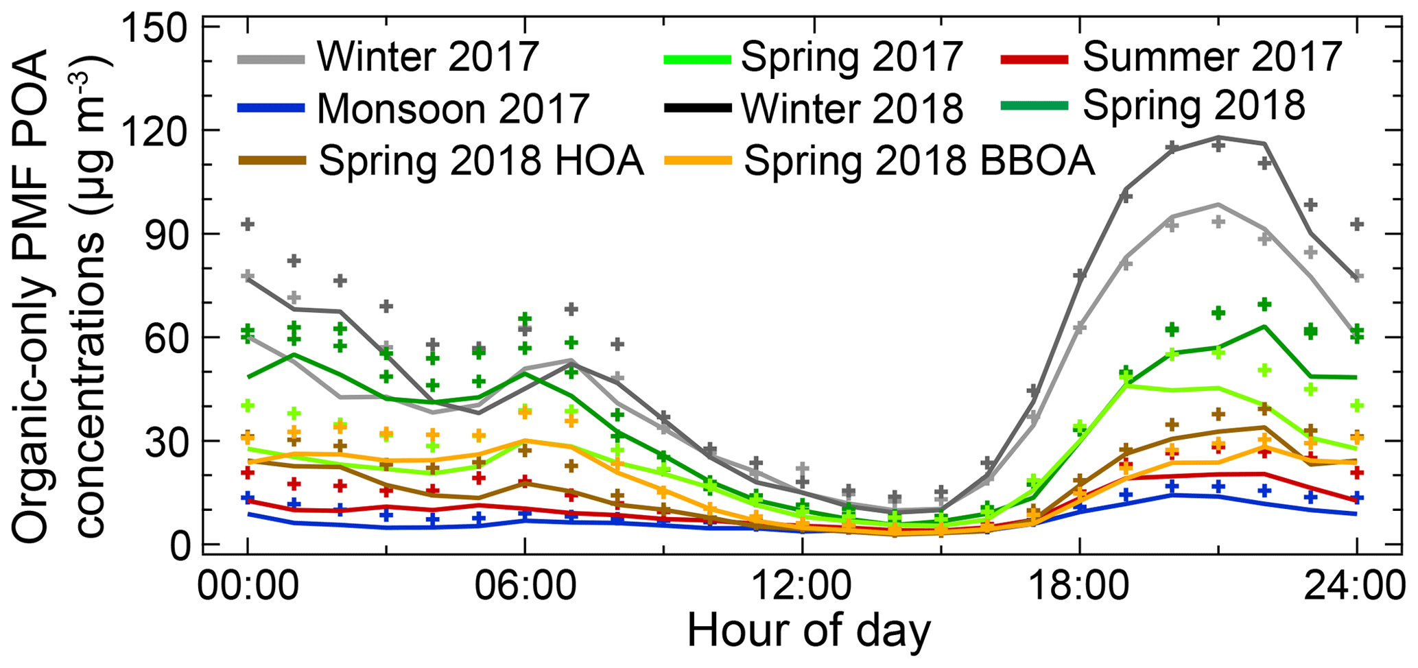
Figure 3Seasonally representative diurnal mean (+) and median concentrations (lines) of POA from organic-only PMF analysis. This figure shows that POA exhibits extreme diurnal variations and displays two peaks, corresponding to the early morning and late evening traffic hours.
Additionally, the lower temperatures in the mornings and evenings of winter and spring seasons (Figs. 3 and S15) also appear to play a role in generating POA peaks at these times. For example, the mean POA concentrations for the coolest 20 % of the dataset (mean temperature of 12.5 ∘C) were ∼53 µg m−3, approximately 3 times as high as the POA concentration for all other hours (mean temperature of 28 ∘C; mean POA of ∼19 µg m−3; Fig. S16c). Finally, the differences in POA diurnal minima across seasons are much smaller than the differences in diurnal peaks – the POA diurnal minimum decreases from ∼10–12 µg m−3 in winter to ∼4 µg m−3 in the monsoon season, and all seasons seem to approach similar baseline concentrations in the afternoon. According to our analysis using the volatility basis set (VBS) (Donahue et al., 2006), differences in observed concentrations in summer and winter can be explained by thermodynamics (equilibrium partitioning) and meteorology (PBLH and VC) alone, suggesting that sources of POA in Delhi may be similar in all seasons. The detailed methodology and results of the VBS analysis are presented in the Supplement (Fig. S17; Sect. S2 – VBS Application).
With regard to interannual variability, we observe notable consistency between daytime POA profiles in winter and spring 2017 and 2018 (09:00–17:00 LT). However, at night and in the early morning, POA concentrations increased in both seasons in 2018 by as much as ∼30 µg m−3. It is well known that the median is robust against extremes and the arithmetic mean (AM) is not. Thus, the relative difference between seasonally averaged mean and median is a qualitative measure of the influence of pollution episodes. Additionally, the magnitude of the standard deviation (SD) relative to the arithmetic mean and the magnitude of the geometric standard deviation (GSD) relative to the geometric mean (GM) are also evidence of episodic behavior. Indeed, based on these metrics of gauging the influence of episodes, POA is influenced by episodic events in the early morning hours in all seasons (Table 3; Fig. 3). These episodes increase mean POA concentrations over the corresponding median by as much as 20 µg m−3, with the largest episodic events occurring in winters. In relative terms, the largest difference is in summer, when mean POA exceeds the median by as much as 55 %. Similarly, though the seasonal AM and GM for POA are generally smaller than the AM and GM for OOA, their corresponding GSD and SD are larger. This difference is particularly stark in colder months, with the POA SD being almost twice the OOA SD, despite a similar AM. While ubiquitous temporally varying sources such as traffic and cooking are important contributors to the overall POA diurnal patterns, they have stable patterns within seasons, associated with working hours and meal consumption. The occurrence of pollution episodes in POA could be a consequence of temperature-related biomass and trash burning (colder periods of day and/or year), agricultural burning (related to the rabi – winter planting and summer harvesting – and kharif – monsoon planting and autumn harvesting – crop harvesting), fireworks, and bonfires (festivals, e.g., Lohri). POA is the largest contributor to PM during these episodes at our site; e.g., for extreme conditions where NR-PM1 exceeded 200 µg m−3, POA accounted for, on an average, 34 % of the NR-PM1 mass (Fig. S18).
It is also important to point out the differences in the HOA and BBOA factors identified in spring 2018 (Figs. 3 and S2f and g). Both HOA and BBOA exhibit episodes in the early morning hours of the day, with higher BBOA concentrations than HOA, and the BBOA contribution to total organic mass as high as 38 %. In the evening and at night, however, HOA is the larger of the two, contributing as much as 42 % to total organic mass. Both components display strong diurnal behavior.
3.2 Oxygenated organic aerosol (OOA)
3.2.1 Organic-only PMF mass spectra and diurnal patterns
Here, we discuss the mass spectral profiles of oxygenated organic aerosol from the seasonal organic-only PMF analysis as well as the combined organic–inorganic PMF analysis. As shown in Fig. 1b, the observed OOA MS profile averaged across seasons is in line with the reference OOA profile. In every season, mass spectra of the OOA factors in organic-only PMF correlate strongly with the reference OOA factor (R>0.95; Fig. S1a–f). The mass spectral profiles for the OOA factor in all seasons are provided in Fig. S5a–f. A large fractional contribution at m∕z 44 is a signature of the OOA factor. The fragment dominates contributions at m∕z 44 compared to other fragments and is produced by the thermal decarboxylation and ionization-induced fragmentation of carboxylic acids (Takegawa et al., 2007). The large fractional contribution at m∕z 44 is beyond 1 SD from the mean of the reference spectrum for most seasons (Fig. S5a–f). This higher contribution at m∕z 44 could be a result of rapid photochemical processing of fresh emissions and/or regional transport of aerosol to the receptor site. The vicinity of the site to local sources suggests that rapid photochemical processing may be more important in causing the high m∕z 44.
The organic-only PMF-based OOA diurnal time series patterns exhibit high interseasonal, limited diurnal, and minimal interannual variability between the winters and springs of 2017 and 2018 and are not influenced by episodic pollution events (Table 3; Fig. 4). Mean and median OOA concentrations, similar in magnitude at most times of the day in every season, increase during the morning, dip midday, and then increase again at night. At nighttime, OOA concentrations remain stable for several hours into the next day and then increase in the early morning. OOA concentrations increase in the morning hours (∼ 05:00–09:00 LT) despite increasing atmospheric mixing, pointing to photochemical formation related to primary emissions from traffic and other sources. The midday dip is likely associated with increasing atmospheric mixing and perhaps a reduction in daytime primary emissions. In contrast, nocturnal OOA concentrations are considerably less variable up to about 04:00–05:00 LT, perhaps representing a lower production rate in the absence of photochemistry. Overall, the timing of local primary emissions, meteorology, and boundary layer dynamics are likely responsible for differing behavior at different times of the day.
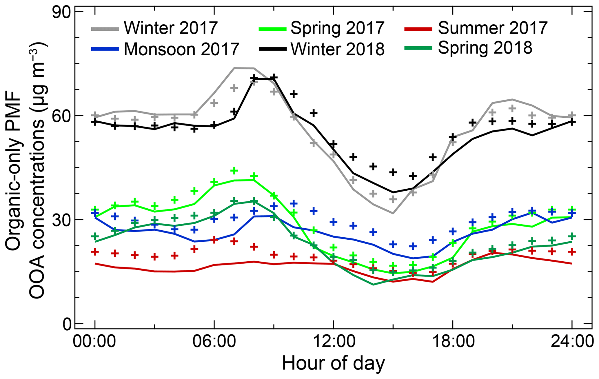
Figure 4Seasonally representative diurnal mean (+) and median concentrations (lines) of OOA from organic-only PMF analysis. This figure shows the higher concentrations of OOA in winters compared to other months and the relatively stronger diurnal variations in winters and springs compared to other seasons.
The diurnal variations in the OOA concentrations are stronger in winter (peak concentration ∼1.9–2.3 times the midday concentration) than in the summer and monsoon season (peak concentration ∼1.6–1.7 times midday concentration). Also, there is a strong seasonality of the factor, with diurnal peak OOA concentrations in winter being nearly 1.7 times those in spring and ∼2.9–3.6 times those during the summer. Nevertheless, diurnal variations in OOA are weaker than their POA counterparts across seasons. Apart from a weaker diurnal variation, the daytime peaks in OOA are larger than nighttime peaks, and diurnal minima in OOA concentrations vary substantially across seasons. As Fig. 4 shows, absolute OOA concentrations have large differences between winters and other seasons. In winters, the mean and median OOA concentrations never dip below 30 µg m−3, whereas in other seasons they do not increase above 30 µg m−3 except for early morning and at night in the spring and monsoon season. As for interannual variability, winter and spring 2018 exhibit variations similar to the respective seasons in 2017.
Except for a brief period in the summer morning, we observe small differences between median and mean OOA concentrations at different hours of the day across seasons (Fig. 4). Similar conclusions can be drawn from the magnitude of SD compared to AM and GSD compared to GM (Table 3); while seasonal AM and GM for OOA are generally larger than AM and GM for POA, their corresponding SD and GSD are smaller. Concentrations of OOA do not increase substantially during pollution episodes, thereby showing different behavior than POA (Sect. 3.1).
3.2.2 Combined organic–inorganic PMF mass spectra and diurnal variation
Incorporating mass spectral data for inorganics in PMF allows further separation of OOA into AS-OOA, AN-OOA, and AC-OOA – a result likely arising from similar volatility of the organic and inorganic components. In this section, we show that chloride, nitrate, and sulfate measured at the site are largely inorganic – as indicated by combined organic–inorganic PMF analysis which groups these species into factors with ammonium. In previous work, OOA associated with ammonium nitrate usually has a mass spectrum showing higher fractional contribution at m∕z 43 (mostly C2H3O+) than m∕z 44 (), where m∕z 43 is believed to be associated with non-acid oxygenates (Ng et al., 2010). Additionally, these organic aerosols generally have time series reflecting semi-volatile behavior and are labeled semi-volatile oxygenated organic aerosol (SVOOA; Zhang et al., 2011). In this study, while AN-OOA exhibits semi-volatile behavior (Fig. 5a), the distribution of AN-OOA profiles and reference SVOOA are different (R<0.8; all seasons; Fig. S7a–f). Instead, the relative mass spectral contributions are in line with the reference OOA and the LVOOA profiles (R>0.95; Figs. S7a–f and S19–S20a–f). The strong mass spectral correlation of AN-OOA with reference LVOOA hints at rapid photochemical aging of aerosols in Delhi so that freshly formed oxidized aerosols have a high oxidation state. The mass spectrum of AS-OOA also compares well to the reference OOA and LVOOA profiles (R>0.95, all seasons; Figs. S7a–f, S21–22a–f). AN-OOA has higher mean mass spectral contribution at m∕z 43 compared to AS-OOA; however, the mass spectral contribution at m∕z 44 is higher in AS-OOA. Additionally, at most high m∕z values between 70 and 120, AN-OOA displays higher contributions than AS-OOA, which is likely a result of less processing (Fig. S23a and b; Ng et al., 2010). AS-OOA profiles have a higher contribution at other prominent lower m∕z values, such as 17, 24, 41, and 55, as well.
The combined organic–inorganic PMF-based AN-OOA and AS-OOA show different time series patterns which change both diurnally and seasonally, pointing to the semi-volatile behavior of AN-OOA and suggesting the potential influence of aqueous-phase chemistry in the formation of AS-OOA at high relative humidity (RH; Fig. 5a and b). Based on the peak-to-minimum ratio in diurnal variations, AN-OOA shows stronger variations than OOA and AS-OOA (Fig. 5a and b). Like OOA from organic-only PMF analysis, the smaller nighttime increase in AN-OOA compared to the daytime peak is likely due to the minimal photochemical formation at night. Also like OOA, concentrations of AN-OOA are higher in winter than in other seasons, with concentrations never dipping below 12.5 µg m−3 in winters. Among other seasons, AN-OOA concentrations exceed this value only in spring mornings. Within 2017, the diurnal patterns and the absolute AN-OOA concentrations change dramatically. In winters, summers, and monsoons, diurnal peak AN-OOA concentrations are ∼2–5 times the diurnal minima; in springs, this ratio increases to ∼6–8 times. In terms of absolute variations in meteorological variables such as temperature, RH, wind speed, and VC, spring shows the most variability (Fig. S15). These variations might be causing the large peak-to-minimum ratio and the sudden drop in AN-OOA concentrations from winter to spring. The two winters and springs show very similar AN-OOA concentration variations. The mean–median difference, GSD versus GM, and SD versus AM point to episodic behavior in all seasons except winters, possibly due to the semi-volatile behavior of AN-OOA leading to its evaporation at higher temperatures each day (Table 4).
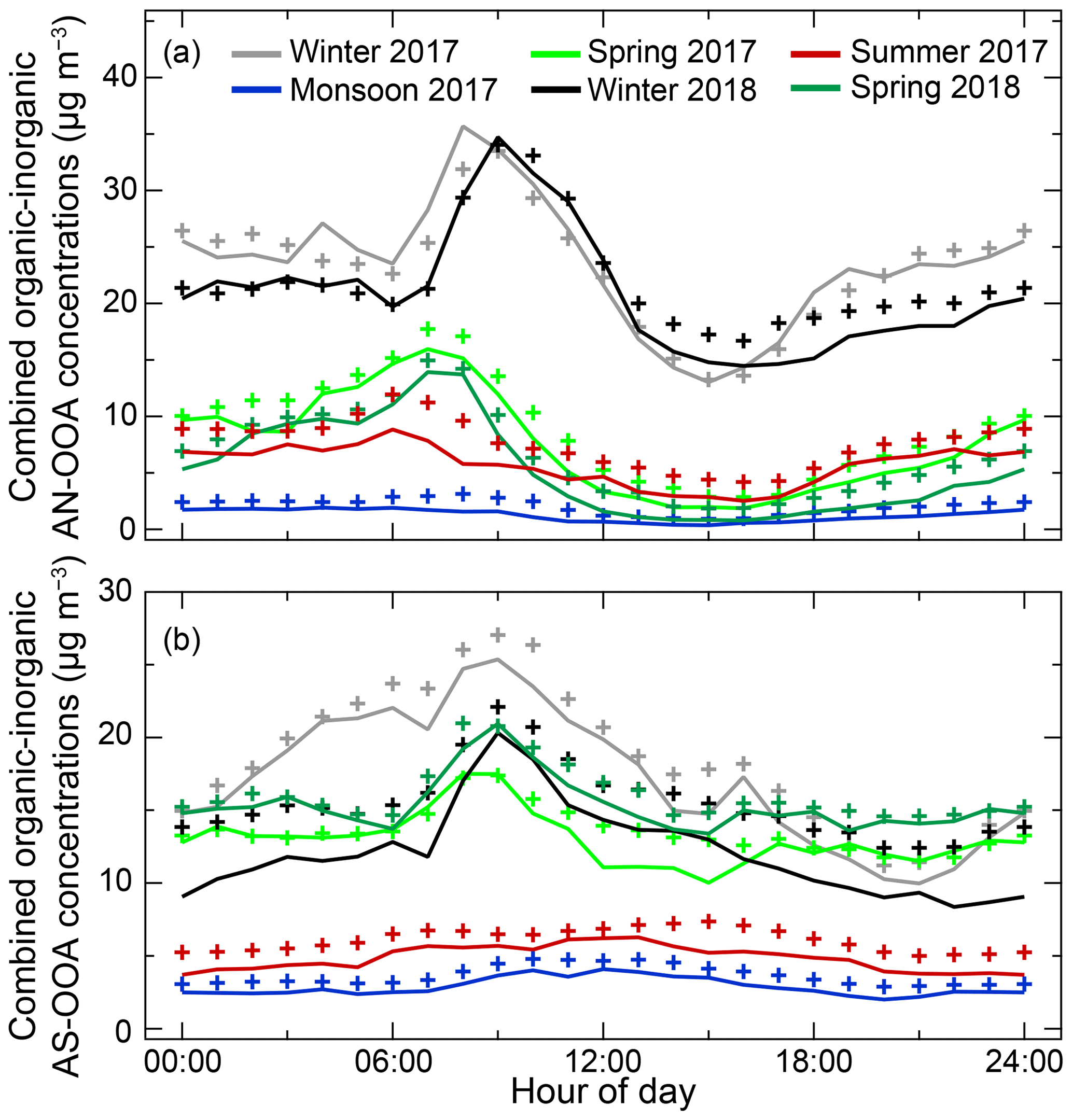
Figure 5Seasonally representative diurnal mean (+) and median (lines) concentrations of (a) AN-OOA and (b) AS-OOA from organic–inorganic combined PMF analysis. Compared to AN-OOA, AS-OOA concentrations remain relatively stable throughout the day, particularly in warmer months.
On the other hand, AS-OOA exhibits more flat profiles, especially in the warmer months, with no prominent troughs and a single morning crest only in the colder seasons (winters and springs; Fig. 5b). Concentrations in winters and springs peak diurnally between 09:00 and 10:00 LT, at ∼2.0–2.5 times the diurnal minima in both winters and ∼1.5–1.8 times in springs. Warmer seasons have similar peak-to-minima ratios of ∼1.5–1.7 times in summer and ∼1.7–2.0 times in monsoon but exhibit more flat profiles in terms of absolute AS-OOA concentrations, with a mean and median always less than 8 µg m−3. Additionally, high RH conditions generally occur during winter, spring, and the monsoon season (Fig. S15). Very humid conditions are associated with especially high AS-OOA concentrations. For example, for the highest decile of RH (RH ∼ 90 %–100 %), the mean AS-OOA concentration (∼6.4 µg −3) exceeds the mean of the corresponding AS-OOA concentrations for conditions where RH < 90 % (∼4.6 µg m−3) by ∼50 % (Fig. S24d). Similar behavior has been observed for the ammonium sulfate aerosols previously measured in Delhi and elsewhere, particularly in the presence of high organic concentrations, and has been attributed to aqueous-phase chemistry (Hu et al., 2011; Wang et al., 2016; Jaiprakash et al., 2017; Sarangi et al., 2018; Wang et al., 2018). Nevertheless, such a correlation does not imply causation; meteorological variables are confounded with each other and with other temporal cycles. The flat and lower AS-OOA concentrations during the rest of the day are likely an indicator of the contribution of regional sources to AS-OOA. AS-OOA diurnal profiles capture important processes such as nighttime secondary formation that are perhaps related to biomass-burning emissions (winter 2017), morning peaks hinting at the possibility of rapid secondary formation from traffic and biomass-burning emissions (winters and springs of 2017 and 2018), and prominent nighttime episodes (winter 2018). The interannual behavior of AS-OOA shows a decrease in the winter median throughout the day in 2018 compared to 2017 (lower by as much as 9 µg m−3) and an increase in spring 2018 median AS-OOA concentrations compared to the median in spring 2017 (higher by as much as ∼4 µg m−3). The mean–median difference also suggests some midday episodes in spring 2017; these episodes are not observed in spring 2018. Overall, AS-OOA is less volatile than AN-OOA and shows weaker episodic behavior based on AM versus GM, SD versus AM, and GSD versus GM (Table 4).
Broadly speaking, springs have a larger AS-OOA-to-AN-OOA ratio relative to the winters and summer. This behavior is likely associated with the transitional meteorology of the spring period, where relatively low temperatures and weak atmospheric mixing coincide with higher photochemistry and relative humidity. Also, GM and median AN-OOA levels in Delhi are higher than AS-OOA only in winters, pointing to the strong influence of temperature on PM formation (the evaporation of semi-volatile compounds in warmer periods) and the importance of less photochemistry in winters. To summarize, despite overall consistency across seasons for OOA, its components AN-OOA and AS-OOA show very different behavior which changes both diurnally and seasonally.
Akin to the associations with ammonium nitrate and ammonium sulfate, some organic components also associate with ammonium chloride (Fig. S7a–f). These organics (AC-OOA) account for 17 %–23 % of the mass of this factor. The median fraction of organics associated with this factor does not exceed 4 %. The mass spectra of these organics resemble oxidized biomass-burning aerosol (higher fraction of organics at m∕z values 60 and 73 than reference SVOOA profile; Figs. S7a–f and S25a–h). These organics may be associated with the AC factor due to their semi-volatile behavior. Indeed, chloride has been used as a tracer for semi-volatile OOA (Zhang et al., 2011). Additionally, chloride has been used as a tracer for biomass burning, specifically agricultural burning, and more recently has also been detected in plastic burning (Li et al., 2014a, b; Kumar et al., 2015; Fourtziou et al., 2017). However, as Fig. S6a–b and e–f show, for the four seasons (winters 2017 and 2018, springs 2017 and 2018), when significant chloride mass is detected in the particulate phase, the time series of the biomass-burning tracers; the aethalometer-derived biomass-burning component of black carbon, BCBB; and the difference between UVPM and BC, ΔC; do not correlate with this AC factor. Also, the highest 10 % of concentrations of this AC factor (>87 µg m−3) are associated with a strong N–NW wind component – this directionality behavior is strongest among all PMF components (Fig. S26a–e). Other OOA components also show similar directionality with weaker strength in the N–NW direction (Fig. S26b and d). In contrast to the OOA components, extreme POA concentrations are associated with a relatively broad range of wind directions (Fig. S26c). This observation suggests that long-range transport from the prevailing N–NW wind direction may be more important for OOA-associated components than for POA. Since Delhi is in an especially ammonia-rich environment (Warner et al., 2017; Van Damme et al., 2018), these observations also suggest that ammonium chloride forms from the interaction of upwind chloride sources and fertilizer emissions. One logical source of chloride emissions would be the industrial use of hydrochloric acid (Jaiprakash et al., 2017).
Considering that the combined organic–inorganic PMF results cluster nitrate, chloride, and sulfate with ammonium, our findings suggest that nitrates, chlorides, and sulfates measured by the ACSM in New Delhi are dominated by inorganics, particularly at higher concentrations. This finding is consistent with results from analysis based on tracer ratios. The ON method, developed by Farmer et al. (2010), estimates the organic nitrate (ON) contribution in the NO3 detected by online mass spectrometers such as the AMS based on the ratio of NO3 fragments at m∕z 30 to m∕z 46. The higher the value relative to the pure ammonium nitrate calibration, the greater the importance of organonitrates. The ratio of m∕z 30 to m∕z 46 increases from winter to the monsoon season and does not exceed the calibration ratio (3.6) in winters, pointing to a negligible fraction of organonitrates in winters. Similarly, Wang and Hildebrandt Ruiz (2017) use the correlation of chloride mass at m∕z 36 to organic mass for evaluating the presence of organochlorides. We observe that chloride m∕z 36 is very weakly correlated to organics, pointing to the dominance of inorganic chlorides. Finally, Hu et al. (2017) suggest use of the SO+ to ratio to estimate the presence of organosulfur species. The range of seasonally representative diurnal median across seasons is 2.4–4.1, agreeing very well with the median values obtained with pure ammonium sulfate calibrations (3.0). This result points to the dominance of inorganic sulfate over organosulfates across seasons. Although the diurnal patterns are stable across seasons, there is a slight upward shift in the median ratio from winter 2017 to spring 2018, pointing to a possible change in the importance of organosulfates.
To summarize, our findings indicate that AN-OOA shows stronger diurnal variability than AS-OOA, and the ratio of AS-OOA to AN-OOA is high in spring, likely due to transitional meteorology. Compared to other factors, AS-OOA concentrations show a strong association with high RH, possibly a consequence of aqueous-phase chemistry. While chloride has been used as a tracer for biomass burning, we do not see any correlation with the aethalometer-derived biomass-burning tracers and suspect chloride to be of an industrial origin. Finally, based on PMF results and tracer ratios and correlations for organic nitrates, chlorides, and sulfates, these species are principally inorganic.
3.3 Primary versus secondary organics
In this section, we summarize the contributions of organics as either primary or secondary using the PMF results. We show that (i) primary emissions are more important in high PM pollution periods, (ii) secondary organic aerosols dominate average concentrations year-round, and (iii) a modified tracer-based organic component evaluation could provide real-time source apportionment of POA and SOA for Delhi (Figs. 6a and b and S27–28).

Figure 6(a) Diurnal mean and median composition of POA from organic-only PMF analysis. Spring 2018 has a relatively higher POA fraction due to the unmixing of a separate BBOA profile. (b) Diurnal mean (+) and median (lines) fraction of OOA from organic-only PMF analysis in different seasons. Fractional contributions vary between 32 % and 80 % except spring 2018. This is likely due to the separation of BBOA mixed into the oxidized organics in spring 2018.
For fractional POA contributions, the nighttime peak between 18:00 and 22:00 LT is larger than the daytime peak between 05:00 and 08:00 LT, likely due to more photochemistry during the day (Fig. 6a). The diurnal minima in the variations occur between 12:00 and 15:00 LT in all seasons, likely due to a combination of reduced sources, increased ventilation, and higher temperatures (Fig. 6a). For winter 2017, although the fraction of POA is generally less than 50%, it nears or exceeds the halfway mark during the early morning traffic hours (06:00–08:00 LT) and for most hours in the evening and at night (17:00–01:00 LT), with similar behavior persisting across seasons. These time windows also correspond to periods with the highest POA and highest total concentrations, pointing to the importance of local, primary emissions in the high-pollution periods, within a day, within each season, and across seasons (Fig. S18). Relative to colder seasons of winter and spring, warmer months exhibit similar midday POA fractions but diverging lower nighttime fractions. The spring 2018 POA fraction varies between 34 % and 75 %, higher than the winters of 2017 and 2018, spring 2017 (20 %–68 %), and summer 2017 and the monsoon season of 2017 (23 %–53 %). Fractional contributions of OOA to total NR-PM1 exhibit a very similar timing of crests and troughs across seasons (Fig. 6b). However, OOA fractions for different seasons converge in the middle of the day and diverge in the early morning and at night, with nighttime fractions in colder months generally lower than the warmer months. This result likely reflects the generally greater influence of primary emissions at night and during colder months. The diurnal OOA fractions peak between 14:00 and 16:00 LT at ∼66 %–80 %. The profiles rapidly descend to diurnal minima between 25 % and 51 % between 19:00 and 20:00 LT, likely due to lowered photochemistry and enhanced primary source strength. As for interannual variability between the winters of 2017 and 2018, winter 2018 has lower OOA fractions, particularly at night, by as much as 14 %. Further, springs of 2017 and 2018 show large differences in the early morning and at night, with OOA in 2018 always contributing less (up to 26 % less around midnight). This difference could, in part, be due to the separation of a BBOA factor in spring 2018 that allows deconvolution of the biomass-burning component. Despite the changes, the diurnal patterns remain consistent interannually.
We have also compared organic-only PMF results with a modified tracer-based organic component evaluation (Ng et al., 2011a). The previously deployed tracer approach utilizes linear scaling of mass at specific m∕z values to estimate the total mass of each of the three factors – HOA, BBOA, and OOA. Since organic-only PMF mostly yields two factors – proxies for primary and secondary aerosols, we compare primary organic aerosols (POA = HOA + BBOA in our analysis) and secondary organic aerosols (OOA) only. However, for our measurements, this results in the total mass estimated using the tracer-based approach substantially different from the actual organic mass (POA: slope ∼ 0.29, intercept ∼ 5.4, R2∼0.76; OOA: slope ∼ 0.41, intercept ∼ 17.3, R2∼0.30; Fig. S27). When we enforce a mass closure on the factors, the tracer-based factors are strongly linearly correlated with results from the organic-only PMF with slopes close to 1 (POA: slope ∼ 0.91, intercept ∼ −3.7, R2∼0.96; OOA: slope ∼ 1.09, intercept ∼ 3.9, R2∼0.94; Fig. S28). Given that the tracer-based approach can be conducted almost instantly, this approach has the potential to be an effective real-time source apportionment approach to separate primary from secondary organic aerosol in Delhi.
3.4 Factors influencing organic aerosol concentrations and composition
3.4.1 Effect of meteorological variables on interannual variability
In this section, we test the association of the interannual increase in concentrations in the winters and springs of 2018 compared to 2017 with meteorological variables. Apart from source effects, the changes can be a consequence of changing wind direction, wind speed, temperature, RH, and boundary layer height. Here, we compare the seasonally averaged diurnal patterns of these variables (Fig. S29a–d). RH averaged over 2017 winter is up to 10 % higher compared to winter 2018 (Fig. S29a). However, RH is not strongly correlated with changes in pollutant concentrations (Fig. S24). At the same time, the temperature between the two winters is within 2 ∘C of each other (Fig. S29b). In spring, RH is within 6 % and temperature is within 4 ∘C at all hours. Diurnal patterns of wind direction are similar in 2017 and 2018, except in the middle of the day, when there is a significant shift of about 28∘ from N–NW to N–NE in winter (Fig. S29c). Between springs, there is a slight shift of about 14∘ towards N–NE late in the evening and night between 20:00 and 24:00 LT. Ventilation coefficients are consistent across the 2 years, except at night – nighttime median VCs are lower by as much as 80 % in winter and spring 2018 (Fig. S29d). Thus, a lower VC for hours of the day when HOA and BBOA are most important could be a key reason behind their higher concentrations. The increase could also be due to an enhancement of sources. In winters, it could also be attributed to the extra period sampled – winter 2018 samples between 21 December and 14 January, a period missed in winter 2017.
3.4.2 Effect of ventilation-related variables on factor concentrations
The association of ventilation-related variables with combined organic–inorganic PMF factors shows that (i) wind speed is not strongly correlated with pollution loading and (ii) boundary layer dynamics seem to regulate all components but to different extents (Fig. S30–32a–e). For all PMF factors, concentrations associated with the lower eight deciles of wind speed (up to ∼3.5 ms−1; ∼80 % of the dataset) show either minimal or no decrease (Fig. S30a–e), while total NR-PM1 shows a subtle decreasing trend with higher wind speed. This observation is important and points to the limited importance of winds in providing “ventilation”. At higher speeds, winds seem to decrease concentrations of the primary components – POA and AC – stronger than the oxidized components. The factors respond contrastingly to the other component important for ventilation, the planetary boundary layer height (PBLH; Fig. S31a–e). Going from the lowest to the highest deciles in PBLH, concentrations of all PMF factors decrease, with especially sharp drops in the first few deciles of PBLH (<100 m), where inversion conditions exert a strong control on concentrations of all species. The anticorrelations with wind speed and PBLH have been observed previously, albeit for PM2.5 and BC concentrations (Guttikunda and Gurjar, 2012; Tiwari et al., 2013). The temperature and ventilation coefficient are correlated (R∼0.6), which implies that the association with boundary layer height is likely convoluted with an association with temperature. Finally, concentrations of PMF factors decrease with an increasing ventilation coefficient, with somewhat larger drops in the concentrations of primary components in comparison to secondary components (Fig. S32a–e).
This study provides long-term source apportionment results for a receptor site in New Delhi, the most polluted megacity in the world. For the first time, highly time-resolved data are available for understanding diurnal patterns and seasonal and interannual changes between the winters and springs of 2017 and 2018 of submicron primary and secondary aerosols. Organic-only PMF analysis yields two to three factors – POA (HOA + BBOA) and OOA in every season and HOA and BBOA separating as factors only in spring 2018. Among factors occurring in every season, POA exhibits the strongest diurnal patterns, with the nighttime peak being much larger than the daytime peak. The combined organic–inorganic PMF analysis allows separation of oxygenated organic aerosols into components based on association with ammonium nitrate and ammonium sulfate. The two components display different diurnal patterns, with AN-OOA showing relatively stronger diurnal patterns and AS-OOA displaying more flat profiles with a sharp rise and descent in the middle of the day, likely associated with photochemical formation. AS-OOA shows a sharp increase in concentrations, especially at high RH, in line with formation influenced by aqueous-phase chemistry. AN-OOA mass spectral profiles are very similar to reference LVOOA profiles, despite the vicinity to local sources, pointing to the rapid processing of aerosols in Delhi. Chloride, nitrate, and sulfate are mostly inorganic. Analysis using the volatility basis set suggests that differences in temperature and, therefore, equilibrium partitioning, can explain differences in observed winter and summer concentrations. While the temperature and ventilation coefficient play a crucial role in determining the organic presence in gas or aerosol phase, the N–NW direction is associated with a significant fraction of >90th percentile events for all OOA-associated-components. In contrast to other variables that control atmospheric ventilation (e.g., PBLH), variation in wind speeds had at most a minimal effect on factor concentrations. Observations indicate that regional OA and ammonium chloride contribute substantially to air pollution in Delhi. Further, primary aerosols such as POA and AC increase, whereas secondary aerosols such as AN-OOA and AS-OOA stabilize, in the high-pollution periods. Thus, primary species are more important contributors to the high pollution episodes in Delhi, and secondary organics dominate year-round fractional contributions to total organics.
The current Indian legislative and legal framework tasks the responsibility of managing air pollution in Delhi to the Environmental Pollution (Prevention & Control) Authority. The Graded Action Response Plan (GRAP) currently in place accounts for a multitude of local and regional sources contributing to air pollution in Delhi (Ministry of Environment, Forest & Climate Change, Government of India, 2018). Because many bottom-up source apportionment efforts for Delhi are based on local-scale (<50–100 km) inventories of primary emissions, they may neglect the important contributions of regionally transported primary and secondary aerosol from upwind regions. Here, we demonstrate the importance of secondary aerosol formed via atmospheric processing. Nevertheless, our results are in broad agreement with these inventories: (1) colder seasons are accompanied by higher concentrations and more diverse sources, including higher biomass-burning emissions, (2) a significant aerosol mass fraction in Delhi is attributable to non-local sources, and (3) industries are a significant source of fine particulate matter (Guttikunda and Calori, 2013; IIT Kanpur, 2016; ARAI and TERI, 2018). However, the lack of consistent emission inventories limits the feasibility of action plans like GRAP, given that their implementation restricts economic activity (CEEW, 2019). The results presented here capture the complexity of aerosols in Delhi by speciating them into different chemical categories and identifying associations of those components with each other and meteorological variables and evaluating their behavior at different times of the day and the year. Because the data presented are highly time-resolved, they can provide critical insight into the diverse sources that contribute to pollution loadings, and similar techniques could be used to measure the efficacy of air pollution regulatory actions. Results from this work address several pressing requirements for air quality management in Delhi, including a real-time source apportionment approach for organics, evidence for extremely high chloride concentrations associated with industrial sources, and evidence for primary components dominating high pollution episodes and secondary components dominating seasonal averages. Future work could utilize these speciated measurements to delve into the identification of potential source locations using back-trajectory analysis.
| AC | Ammonium chloride |
| ACOOA | Oxygenated organic aerosol mixed with ammonium chloride |
| AC-OOA | Oxygenated organic aerosol associated with ammonium chloride |
| ACSM | Aerosol Chemical Speciation Monitor |
| AMS | Aerosol mass spectrometer |
| AN | Ammonium nitrate |
| ANOOA | Oxygenated organic aerosol mixed with ammonium nitrate |
| AN-OOA | Oxygenated organic aerosol associated with ammonium nitrate |
| AS | Ammonium sulfate |
| ASOOA | Oxygenated organic aerosol mixed with ammonium sulfate |
| AS-OOA | Oxygenated organic aerosol associated with ammonium sulfate |
| BBOA | Biomass-burning organic aerosol |
| BC | Black carbon |
| CO | Carbon monoxide |
| CPCB | Central Pollution Control Board |
| DAS | Delhi Aerosol Supersite |
| E-AIM | Extended aerosol inorganics model |
| GRAP | Graded Action Response Plan |
| HOA | Hydrocarbon-like organic aerosol |
| HYSPLIT | NOAA Hybrid Single Particle Lagrangian Integrated Trajectory Model |
| IIT Delhi | Indian Institute of Technology Delhi |
| LT | Local time |
| LVOOA | Low-volatility oxygenated organic aerosol |
| MS | Mass spectra |
| NCR | National Capital Region |
| N–NW | North–northwest |
| N–NE | North–northeast |
| NR-PM1 | Non-refractory submicron particulate matter |
| ON | Organic nitrate |
| ON | Method to estimate organonitrate fraction using fragment ratio of NO3 30 to 46 |
| OOA | Oxygenated organic aerosol |
| PBLH | Planetary boundary layer height |
| PET | PMF evaluation tool |
| PAHs | Polycyclic aromatic hydrocarbons |
| PM1 | Submicron particulate matter |
| PM10 | Particulate matter smaller than 10 µm in diameter |
| PMF | Positive matrix factorization |
| POA | Mixed HOA and BBOA |
| RH | Relative humidity |
| SOA | Secondary organic aerosol |
| UVPM | Ultraviolet-absorbing particulate matter |
| VBS | Volatility basis set |
| VC | Ventilation coefficient |
Data published in this paper's figures and tables are available via the Texas Data Repository (https://doi.org/10.18738/T8/U1BK3K, Hildebrandt Ruiz, 2020). Underlying research data are also available by request to Lea Hildebrandt Ruiz: lhr@che.utexas.edu.
The supplement related to this article is available online at: https://doi.org/10.5194/acp-20-735-2020-supplement.
LHR, JSA, GH, SB, and SG designed the study. SG, SB, PS, and ZA carried out the data collection. SB, KP, DSW, and SG carried out the data processing and analysis. SB, SG, KP, JSA, and LHR assisted with the interpretation of results. All co-authors contributed to writing and reviewing the paper.
The authors declare that they have no conflict of interest.
We are thankful to the Indian Institute of Technology (IIT) Delhi for institutional support. We are grateful to all student and staff members of the Aerosol Research Characterization Laboratory (especially Nisar Ali Baig and Mohammad Yawar) and the Environmental Engineering Laboratory (especially Sanjay Gupta) at IIT Delhi for their constant support. We are thankful to Philip Croteau (Aerodyne Research) for always providing timely technical support for the ACSM.
This material is based on work supported by the Welch Foundation under grant no. F-1925 and the National Science Foundation under grant no. 1653625. Joshua S. Apte was supported by the ClimateWorks Foundation.
This paper was edited by Stefania Gilardoni and reviewed by two anonymous referees.
Aiken, A. C., Salcedo, D., Cubison, M. J., Huffman, J. A., DeCarlo, P. F., Ulbrich, I. M., Docherty, K. S., Sueper, D., Kimmel, J. R., Worsnop, D. R., Trimborn, A., Northway, M., Stone, E. A., Schauer, J. J., Volkamer, R. M., Fortner, E., de Foy, B., Wang, J., Laskin, A., Shutthanandan, V., Zheng, J., Zhang, R., Gaffney, J., Marley, N. A., Paredes-Miranda, G., Arnott, W. P., Molina, L. T., Sosa, G., and Jimenez, J. L.: Mexico City aerosol analysis during MILAGRO using high resolution aerosol mass spectrometry at the urban supersite (T0) – Part 1: Fine particle composition and organic source apportionment, Atmospheric Chemistry and Physics, 9, 6633–6653, https://doi.org/10.5194/acp-9-6633-2009, 2009. a, b
Al-Naiema, I. M., Hettiyadura, A. P. S., Wallace, H. W., Sanchez, N. P., Madler, C. J., Cevik, B. K., Bui, A. A. T., Kettler, J., Griffin, R. J., and Stone, E. A.: Source apportionment of fine particulate matter in Houston, Texas: insights to secondary organic aerosols, Atmos. Chem. Phys., 18, 15601–15622, https://doi.org/10.5194/acp-18-15601-2018, 2018. a, b
Apte, J. S. and Pant, P.: Toward cleaner air for a billion Indians, P. Natl. Acad. Sci. USA, 116, 10614–10616, https://doi.org/10.1073/pnas.1905458116, 2019. a
Apte, J. S., Marshall, J. D., Cohen, A. J., and Brauer, M.: Addressing global mortality from ambient PM2.5, Environ. Sci. Technol., 49, 8057–8066, https://doi.org/10.1021/acs.est.5b01236, 2015. a
ARAI and TERI: Source apportionment of PM2.5 and PM10 of Delhi NCR for identification of major sources, available at: https://www.teriin.org/sites/default/files/2018-08/AQM-SA_0.pdf (last access: 5 November 2019), 2018. a, b
Belis, C., Karagulian, F., Amato, F., Almeida, M., Artaxo, P., Beddows, D., Bernardoni, V., Bove, M., Carbone, S., Cesari, D., and Contini, D.: A new methodology to assess the performance and uncertainty of source apportionment models II: The results of two European intercomparison exercises, Atmos. Environ., 123, 240–250, https://doi.org/10.1016/j.atmosenv.2015.10.068, 2015. a
Bertrand, A., Stefenelli, G., Bruns, E. A., Pieber, S. M., Temime-Roussel, B., Slowik, J. G., Prévôt, A. S., Wortham, H., Haddad, I. E., and Marchand, N.: Primary emissions and secondary aerosol production potential from woodstoves for residential heating: Influence of the stove technology and combustion efficiency, Atmos. Environ., 169, 65–79, https://doi.org/10.1016/j.atmosenv.2017.09.005, 2017. a
CEEW: What is Polluting Delhi's Air? Understanding Uncertainties in Emissions Inventory, available at: https://www.ceew.in/publications/what-polluting-delhi%E2%80%99s-air, last access: 5 November 2019. a
Chowdhury, Z., Zheng, M., Schauer, J. J., Sheesley, R. J., Salmon, L. G., Cass, G. R., and Russell, A. G.: Speciation of ambient fine organic carbon particles and source apportionment of PM2.5 in Indian cities, J. Geophys. Res.-Atmos., 112,D15303, https://doi.org/10.1029/2007JD008386, 2007. a
Conibear, L., Butt, E., Knote, C., Arnold, S. R., and Spracklen, D. V.: Residential energy use emissions dominate health impacts from exposure to ambient particulate matter in India, Nat. Commun., 9, 617, https://doi.org/10.1038/s41467-018-02986-7, 2018. a
Crippa, M., Canonaco, F., Lanz, V. A., Äijälä, M., Allan, J. D., Carbone, S., Capes, G., Ceburnis, D., Dall'Osto, M., Day, D. A., DeCarlo, P. F., Ehn, M., Eriksson, A., Freney, E., Hildebrandt Ruiz, L., Hillamo, R., Jimenez, J. L., Junninen, H., Kiendler-Scharr, A., Kortelainen, A.-M., Kulmala, M., Laaksonen, A., Mensah, A. A., Mohr, C., Nemitz, E., O'Dowd, C., Ovadnevaite, J., Pandis, S. N., Petäjä, T., Poulain, L., Saarikoski, S., Sellegri, K., Swietlicki, E., Tiitta, P., Worsnop, D. R., Baltensperger, U., and Prévôt, A. S. H.: Organic aerosol components derived from 25 AMS data sets across Europe using a consistent ME-2 based source apportionment approach, Atmos. Chem. Phys., 14, 6159–6176, https://doi.org/10.5194/acp-14-6159-2014, 2014. a
Donahue, N. M., Robinson, A. L., Stanier, C. O., and Pandis, S. N.: Coupled partitioning, dilution, and chemical aging of semivolatile organics, Environ. Sci. Technol., 40, 2635–2643, https://doi.org/10.1021/es052297c, 2006. a
Drinovec, L., Močnik, G., Zotter, P., Prévôt, A. S. H., Ruckstuhl, C., Coz, E., Rupakheti, M., Sciare, J., Müller, T., Wiedensohler, A., and Hansen, A. D. A.: The “dual-spot” aethalometer: An improved measurement of aerosol black carbon with real-time loading compensation, Atmos. Meas. Tech., 8, 1965–1979, https://doi.org/10.5194/amt-8-1965-2015, 2015. a
Elser, M., Huang, R.-J., Wolf, R., Slowik, J. G., Wang, Q., Canonaco, F., Li, G., Bozzetti, C., Daellenbach, K. R., Huang, Y., Zhang, R., Li, Z., Cao, J., Baltensperger, U., El-Haddad, I., and Prévôt, A. S. H.: New insights into PM2.5 chemical composition and sources in two major cities in China during extreme haze events using aerosol mass spectrometry, Atmos. Chem. Phys., 16, 3207–3225, https://doi.org/10.5194/acp-16-3207-2016, 2016. a, b
Farmer, D. K., Matsunaga, A., Docherty, K. S., Surratt, J. D., Seinfeld, J. H., Ziemann, P. J., and Jimenez, J. L.: Response of an aerosol mass spectrometer to organonitrates and organosulfates and implications for atmospheric chemistry, P. Natl. Acad. Sci. USA, 107, 6670–6675, https://doi.org/10.1073/pnas.0912340107, 2010. a
Fourtziou, L., Liakakou, E., Stavroulas, I., Theodosi, C., Zarmpas, P., Psiloglou, B., Sciare, J., Maggos, T., Bairachtari, K., Bougiatioti, A., Gerasopoulos, E., Sarda-Estève, R., Bonnaire, N., and Mihalopoulos, N.: Multi-tracer approach to characterize domestic wood burning in Athens (Greece) during wintertime, Atmos. Environ., 148, 89–101, https://doi.org/10.1016/j.atmosenv.2016.10.011, 2017. a
Gani, S., Bhandari, S., Seraj, S., Wang, D. S., Patel, K., Soni, P., Arub, Z., Habib, G., Hildebrandt Ruiz, L., and Apte, J.: Submicron aerosol composition in the world's most polluted megacity: The Delhi Aerosol Supersite study, Atmos.Chem. Phys., 19, 6843–6859, https://doi.org/10.5194/acp-19-6843-2019, 2019. a, b, c, d
GBD MAPS Working Group: Burden of Disease Attributable to Major Air Pollution Sources in India: Special Report 21, available at: https://www.healtheffects.org/publication/gbd-air-pollution-india (last access: 5 November 2019), 2018. a
Goetz, J. D., Giordano, M. R., Stockwell, C. E., Christian, T. J., Maharjan, R., Adhikari, S., Bhave, P. V., Praveen, P. S., Panday, A. K., Jayarathne, T., Stone, E. A., Yokelson, R. J., and DeCarlo, P. F.: Speciated online PM1 from South Asian combustion sources – Part 1: Fuel-based emission factors and size distributions, Atmos. Chem. Phys., 18, 14653–14679, https://doi.org/10.5194/acp-18-14653-2018, 2018. a
Guo, H., Kota, S. H., Chen, K., Sahu, S. K., Hu, J., Ying, Q., Wang, Y., and Zhang, H.: Source contributions and potential reductions to health effects of particulate matter in India, Atmos. Chem. Phys., 18, 15219–15229, https://doi.org/10.5194/acp-18-15219-2018, 2018. a
Guttikunda, S. K. and Calori, G.: A GIS based emissions inventory at 1 km × 1 km spatial resolution for air pollution analysis in Delhi, India, Atmos. Environ., 67, 101–111, https://doi.org/10.1016/j.atmosenv.2012.10.040, 2013. a, b
Guttikunda, S. K. and Gurjar, B. R.: Role of meteorology in seasonality of air pollution in megacity Delhi, India, Environ. Monit. Assess., 184, 3199–3211, https://doi.org/10.1007/s10661-011-2182-8, 2012. a
He, L.-Y., Lin, Y., Huang, X.-F., Guo, S., Xue, L., Su, Q., Hu, M., Luan, S.-J., and Zhang, Y.-H.: Characterization of high-resolution aerosol mass spectra of primary organic aerosol emissions from Chinese cooking and biomass burning, Atmos. Chem. Phys., 10, 11535–11543, https://doi.org/10.5194/acp-10-11535-2010, 2010. a
Hildebrandt Ruiz, L.: Data published in “Sources and atmospheric dynamics of organic aerosol in New Delhi, India: Insights from receptor modeling”, Texas Data Repository, https://doi.org/10.18738/T8/U1BK3K, 2020. a
Hu, D., Chen, J., Ye, X., Li, L., and Yang, X.: Hygroscopicity and evaporation of ammonium chloride and ammonium nitrate: Relative humidity and size effects on the growth factor, Atmos. Environ., 45, 2349–2355, https://doi.org/10.1016/j.atmosenv.2011.02.024, 2011. a
Hu, W., Campuzano-Jost, P., Day, D. A., Croteau, P., Canagaratna, M. R., Jayne, J. T., Worsnop, D. R., and Jimenez, J. L.: Evaluation of the new capture vaporizer for aerosol mass spectrometers (AMS) through field studies of inorganic species, Aerosol Sci. Tech., 51, 735–754, https://doi.org/10.1080/02786826.2017.1296104, 2017. a
IIT Bombay: Development of air pollution source profiles-Stationary sources, available at: https://www.cpcb.nic.in/displaypdf.php?id=U291cmNlLUVta (last access: 5 November 2019), 2008. a
IIT Kanpur: Comprehensive study on air pollution and greenhouse gases (GHGs) in Delhi, available at: http://cerca.iitd.ac.in/files/reports/IITK study 2016.pdf (last access: 5 November 2019), 2016. a, b
Indian National Science Academy: Seasons of Delhi, available at: https://www.insaindia.res.in/climate.php (last access: 25 April 2019), 2018. a
Jaiprakash, Singhai, A., Habib, G., Raman, R. S., and Gupta, T.: Chemical characterization of PM1 aerosol in Delhi and source apportionment using positive matrix factorization, Environ. Sci. Poll. Res., 24, 445–462, https://doi.org/10.1007/s11356-016-7708-8, 2017. a, b, c, d
Jayarathne, T., Stockwell, C. E., Bhave, P. V., Praveen, P. S., Rathnayake, C. M., Islam, M. R., Panday, A. K., Adhikari, S., Maharjan, R., Goetz, J. D., DeCarlo, P. F., Saikawa, E., Yokelson, R. J., and Stone, E. A.: Nepal Ambient Monitoring and Source Testing Experiment (NAMaSTE): emissions of particulate matter from wood- and dung-fueled cooking fires, garbage and crop residue burning, brick kilns, and other sources, Atmos. Chem. Phys., 18, 2259–2286, https://doi.org/10.5194/acp-18-2259-2018, 2018. a
Jimenez group: PMF-AMS Analysis Guide – Jimenez Group Wiki, available at: http://cires1.colorado.edu/jimenez-group/wiki/index.php/PMF-AMS_Analysis_Guide (last access: 25 April 2019), 2018. a
Kumar, S., Aggarwal, S. G., Gupta, P. K., and Kawamura, K.: Investigation of the tracers for plastic-enriched waste burning aerosols, Atmos. Environ., 108, 49–58, https://doi.org/10.1016/j.atmosenv.2015.02.066, 2015. a
Li, J., Song, Y., Mao, Y., Mao, Z., Wu, Y., Li, M., Huang, X., He, Q., and Hu, M.: Chemical characteristics and source apportionment of PM2.5 during the harvest season in eastern China's agricultural regions, Atmos. Environ., 92, 442–448, https://doi.org/10.1016/j.atmosenv.2014.04.058, 2014a. a
Li, J., Wang, G., Aggarwal, S. G., Huang, Y., Ren, Y., Zhou, B., Singh, K., Gupta, P. K., Cao, J., and Zhang, R.: Comparison of abundances, compositions and sources of elements, inorganic ions and organic compounds in atmospheric aerosols from Xi'an and New Delhi, two megacities in China and India, Sci. Total Environ., 476–477, 485–495, https://doi.org/10.1016/j.scitotenv.2014.01.011, 2014b. a
Ministry of Environment, Forest & Climate Change, Government of India: Graded response action plan for Delhi & NCR, available at: http://cpcb.nic.in/uploads/final_graded_table.pdf (last access: 25 April 2019), 2018. a
Mitra, A. and Sharma, C.: Indian aerosols: Present status, Chemosphere, 49, 1175–1190, https://doi.org/10.1016/S0045-6535(02)00247-3, 2002. a
Mönkkönen, P., Uma, R., Srinivasan, D., Koponen, I., Lehtinen, K., Hämeri, K., Suresh, R., Sharma, V., and Kulmala, M.: Relationship and variations of aerosol number and PM10 mass concentrations in a highly polluted urban environment – New Delhi, India, Atmos. Environ., 38, 425–433, https://doi.org/10.1016/j.atmosenv.2003.09.071, 2004. a
Mönkkönen, P., Koponen, I. K., Lehtinen, K. E. J., Hämeri, K., Uma, R., and Kulmala, M.: Measurements in a highly polluted Asian mega city: Observations of aerosol number size distribution, modal parameters and nucleation events, Atmos. Chem. Phys., 5, 57–66, https://doi.org/10.5194/acp-5-57-2005, 2005a. a
Mönkkönen, P., Pai, P., Maynard, A., Lehtinen, K., Hämeri, K., Rechkemmer, P., Ramachandran, G., Prasad, B., and Kulmala, M.: Fine particle number and mass concentration measurements in urban Indian households, Sci. Total Environ., 347, 131–147, https://doi.org/10.1016/j.scitotenv.2004.12.023, 2005b. a
Ng, N. L., Canagaratna, M. R., Zhang, Q., Jimenez, J. L., Tian, J., Ulbrich, I. M., Kroll, J. H., Docherty, K. S., Chhabra, P. S., Bahreini, R., Murphy, S. M., Seinfeld, J. H., Hildebrandt, L., Donahue, N. M., DeCarlo, P. F., Lanz, V. A., Prévôt, A. S. H., Dinar, E., Rudich, Y., and Worsnop, D. R.: Organic aerosol components observed in Northern Hemispheric datasets from aerosol mass spectrometry, Atmos. Chem. Phys., 10, 4625–4641, https://doi.org/10.5194/acp-10-4625-2010, 2010. a, b, c
Ng, N. L., Canagaratna, M. R., Jimenez, J. L., Zhang, Q., Ulbrich, I. M., and Worsnop, D. R.: Real-time methods for estimating organic component mass concentrations from aerosol mass spectrometer data, Environ. Sci. Technol., 45, 910–916, https://doi.org/10.1021/es102951k, 2011a. a, b, c
Ng, N. L., Herndon, S. C., Trimborn, A., Canagaratna, M. R., Croteau, P. L., Onasch, T. B., Sueper, D., Worsnop, D. R., Zhang, Q., Sun, Y. L., and Jayne, J. T.: An Aerosol Chemical Speciation Monitor (ACSM) for routine monitoring of the composition and mass concentrations of ambient aerosol, Aerosol Sci. Tech., 45, 780–794, https://doi.org/10.1080/02786826.2011.560211, 2011b. a
Olson, M. R., Garcia, M. V., Robinson, M. A., Rooy, P. V., Dietenberger, M. A., Bergin, M., and Schauer, J. J.: Investigation of black and brown carbon multiple-wavelength-dependent light absorption from biomass and fossil fuel combustion source emissions, J. Geophys. Res.-Atmos., 120, 6682–6697, https://doi.org/10.1002/2014JD022970, 2015. a
Paatero, P. and Tapper, U.: Positive matrix factorization: A non-negative factor model with optimal utilization of error estimates of data values, Environmetrics, 5, 111–126, https://doi.org/10.1002/env.3170050203, 1994. a
Pant, P. and Harrison, R. M.: Critical review of receptor modelling for particulate matter: A case study of India, Atmos. Environ., 49, 1–12, https://doi.org/10.1016/j.atmosenv.2011.11.060, 2012. a, b
Pant, P., Shukla, A., Kohl, S. D., Chow, J. C., Watson, J. G., and Harrison, R. M.: Characterization of ambient PM2.5 at a pollution hotspot in New Delhi, India and inference of sources, Atmos. Environ., 109, 178–189, https://doi.org/10.1016/j.atmosenv.2015.02.074, 2015. a, b, c, d
Pant, P., Baker, S. J., Goel, R., Guttikunda, S., Goel, A., Shukla, A., and Harrison, R. M.: Analysis of size-segregated winter season aerosol data from New Delhi, India, Atmos. Poll. Res., 7, 100–109, https://doi.org/10.1016/j.apr.2015.08.001, 2016a. a
Pant, P., Guttikunda, S. K., and Peltier, R. E.: Exposure to particulate matter in India: A synthesis of findings and future directions, Environ. Res., 147, 480–496, https://doi.org/10.1016/j.envres.2016.03.011, 2016b. a
Pope, C. A. and Dockery, D. W.: Health effects of fine particulate air pollution: Lines that connect, J. Air Waste Manage. Assoc., 56, 709–742, https://doi.org/10.1080/10473289.2006.10464485, 2006. a
Sandradewi, J., Prévôt, A. S. H., Szidat, S., Perron, N., Alfarra, M. R., Lanz, V. A., Weingartner, E., and Baltensperger, U.: Using aerosol light absorption measurements for the quantitative determination of wood burning and traffic emission contributions to particulate matter, Environ. Sci. Technol., 42, 3316–3323, https://doi.org/10.1021/es702253m, 2008. a
Sarangi, B., Aggarwal, S. G., Kunwar, B., Kumar, S., Kaur, R., Sinha, D., Tiwari, S., and Kawamura, K.: Nighttime particle growth observed during spring in New Delhi: Evidences for the aqueous phase oxidation of SO2, Atmos. Environ., 188, 82–96, https://doi.org/10.1016/j.atmosenv.2018.06.018, 2018. a
Seinfeld, J. H. and Pandis, S. N.: Atmospheric Chemistry and Physics: From Air Pollution to Climate Change, 3rd Edn., Wiley, Hoboken, New Jersey, 2016. a
Sharma, D. N., Sawant, A. A., Uma, R., and Cocker, D. R.: Preliminary chemical characterization of particle-phase organic compounds in New Delhi, India, Atmos. Environ., 37, 4317–4323, https://doi.org/10.1016/S1352-2310(03)00563-6, 2003. a
Sharma, S. and Mandal, T.: Chemical composition of fine mode particulate matter (PM2.5) in an urban area of Delhi, India and its source apportionment, Urban Clim., 21, 106–122, https://doi.org/10.1016/j.uclim.2017.05.009, 2017. a, b
Sharma, S., Mandal, T., Saxena, M., Rashmi, Rohtash, Sharma, A., and Gautam, R.: Source apportionment of PM10 by using positive matrix factorization at an urban site of Delhi, India, Urban Clim., 10, 656–670, https://doi.org/10.1016/j.uclim.2013.11.002, 2014. a
Singh, D., Gadi, R., and Mandal, T. K.: Characterization of particulate-bound polycyclic aromatic hydrocarbons and trace metals composition of urban air in Delhi, India, Atmos. Environ., 45, 7653–7663, https://doi.org/10.1016/j.atmosenv.2011.02.058, 2011. a
Srivastava, A., Gupta, S., and Jain, V.: Source apportionment of total suspended particulate matter in coarse and fine size ranges over Delhi, Aerosol Air Qual. Res., 8, 188–200, https://doi.org/10.4209/aaqr.2007.09.0040, 2008. a
Srivastava, D., Favez, O., Petit, J., Zhang, Y., Sofowotee, U., Hopke, P., Bonnaire, N., Perraudin, E., Gros, V., and Villenave, Albinet, A.: Speciation of organic fractions does matter for aerosol source apportionment. Part 3: Combining off-line and on-line measurements, Sci. Total Environ., 690, 944–955, https://doi.org/10.1016/j.scitotenv.2019.06.378, 2019. a
Stockwell, C. E., Christian, T. J., Goetz, J. D., Jayarathne, T., Bhave, P. V., Praveen, P. S., Adhikari, S., Maharjan, R., DeCarlo, P. F., Stone, E. A., Saikawa, E., Blake, D. R., Simpson, I. J., Yokelson, R. J., and Panday, A. K.: Nepal Ambient Monitoring and Source Testing Experiment (NAMaSTE): emissions of trace gases and light-absorbing carbon from wood and dung cooking fires, garbage and crop residue burning, brick kilns, and other sources, Atmos. Chem. Phys., 16, 11043–11081, https://doi.org/10.5194/acp-16-11043-2016, 2016. a
Sun, Y. L., Zhang, Q., Schwab, J. J., Yang, T., Ng, N. L., and Demerjian, K. L.: Factor analysis of combined organic and inorganic aerosol mass spectra from high resolution aerosol mass spectrometer measurements, Atmos. Chem. Phys., 12, 8537–8551, https://doi.org/10.5194/acp-12-8537-2012, 2012. a, b
Takegawa, N., Miyakawa, T., Kawamura, K., and Kondo, Y.: Contribution of Selected Dicarboxylic and ω-Oxocarboxylic Acids in Ambient Aerosol to the m∕z 44 Signal of an Aerodyne Aerosol Mass Spectrometer, Aerosol Sci. Tech., 41, 418–437, https://doi.org/10.1080/02786820701203215, 2007. a
Tian, J., Wang, Q., Ni, H., Wang, M., Zhou, Y., Han, Y., Shen, Z., Pongpiachan, S., Zhang, N., Zhao, Z., Zhang, Q., Zhang, Y., Long, X., and Cao, J.: Emission characteristics of primary brown carbon absorption from biomass and coal burning: Development of an optical emission inventory for China, J. Geophys. Res.-Atmos., 124, 1879–1893, https://doi.org/10.1029/2018JD029352, 2019. a
Tiwari, S., Srivastava, A. K., Bisht, D. S., Bano, T., Singh, S., Behura, S., Srivastava, M. K., Chate, D. M., and Padmanabhamurty, B.: Black carbon and chemical characteristics of PM10 and PM2.5 at an urban site of North India, J. Atmos. Chem., 62, 193–209, https://doi.org/10.1007/s10874-010-9148-z, 2009. a
Tiwari, S., Srivastava, A., Bisht, D., Parmita, P., Srivastava, M. K., and Attri, S.: Diurnal and seasonal variations of black carbon and PM2.5 over New Delhi, India: Influence of meteorology, Atmos. Res., 125–126, 50–62, https://doi.org/10.1016/j.atmosres.2013.01.011, 2013. a
Ulbrich, I. M., Canagaratna, M. R., Zhang, Q., Worsnop, D. R., and Jimenez, J. L.: Interpretation of organic components from positive matrix factorization of aerosol mass spectrometric data, Atmos. Chem. Phys., 9, 2891–2918, https://doi.org/10.5194/acp-9-2891-2009, 2009. a, b, c
Ulbrich, I. M., Handschy, A., Lechner, M., and Jimenez, J.: AMS Spectral Database, available at: http://cires.colorado.edu/jimenez-group/AMSsd/ (last access: 25 April 2019), 2017. a
Ulbrich, I. M., Handschy, A., Lechner, M., and Jimenez, J.: High-Resolution AMS Spectral Database, available at: http://cires.colorado.edu/jimenez-group/HRAMSsd/ (last access: 25 April 2019), 2018. a
United Nations: World urbanization prospects, available at: https://population.un.org/wup/ (last access: 25 April 2019), 2018. a
Van Damme, M., Clarisse, L., Whitburn, S., Hadji-Lazaro, J., Hurtmans, D., Clerbaux, C., and Coheur, P.-F.: Industrial and agricultural ammonia point sources exposed, Nature, 564, 99–103, https://doi.org/10.1038/s41586-018-0747-1, 2018. a
Wang, D. S. and Hildebrandt Ruiz, L.: Secondary organic aerosol from chlorine-initiated oxidation of isoprene, Atmos. Chem. Phys., 17, 13491–13508, https://doi.org/10.5194/acp-17-13491-2017, 2017. a
Wang, G., Zhang, R., Gomez, M. E., Yang, L., Levy Zamora, M., Hu, M., Lin, Y., Peng, J., Guo, S., Meng, J., Li, J., Cheng, C., Hu, T., Ren, Y., Wang, Y., Gao, J., Cao, J., An, Z., Zhou, W., Li, G., Wang, J., Tian, P., Marrero-Ortiz, W., Secrest, J., Du, Z., Zheng, J., Shang, D., Zeng, L., Shao, M., Wang, W., Huang, Y., Wang, Y., Zhu, Y., Li, Y., Hu, J., Pan, B., Cai, L., Cheng, Y., Ji, Y., Zhang, F., Rosenfeld, D., Liss, P. S., Duce, R. A., Kolb, C. E., and Molina, M. J.: Persistent sulfate formation from London Fog to Chinese haze, P. Natl. Acad. Sci. USA, 113, 13630–13635, https://doi.org/10.1073/pnas.1616540113, 2016. a
Wang, G., Zhang, F., Peng, J., Duan, L., Ji, Y., Marrero-Ortiz, W., Wang, J., Li, J., Wu, C., Cao, C., Wang, Y., Zheng, J., Secrest, J., Li, Y., Wang, Y., Li, H., Li, N., and Zhang, R.: Particle acidity and sulfate production during severe haze events in China cannot be reliably inferred by assuming a mixture of inorganic salts, Atmos. Chem. Phys., 18, 10123–10132, https://doi.org/10.5194/acp-18-10123-2018, 2018. a
Wang, Y., Hopke, P. K., Rattigan, O. V., Xia, X., Chalupa, D. C., and Utell, M. J.: Characterization of residential wood combustion particles using the two-wavelength aethalometer, Environ. Sci. Technol., 45, 7387–7393, https://doi.org/10.1021/es2013984, 2011. a
Warner, J. X., Dickerson, R. R., Wei, Z., Strow, L. L., Wang, Y., and Liang, Q.: Increased atmospheric ammonia over the world's major agricultural areas detected from space, Geophys. Res. Lett., 44, 2875–2884, https://doi.org/10.1002/2016GL072305, 2017. a
World Health Organization: AAP air quality database, available at: http://www.who.int/phe/health_topics/outdoorair/databases/cities/en/ (last access: 25 April 2019), 2018. a, b
Zhang, Q., Alfarra, M. R., Worsnop, D. R., Allan, J. D., Coe, H., Canagaratna, M. R., and Jimenez, J. L.: Deconvolution and quantification of hydrocarbon-like and oxygenated organic aerosols based on aerosol mass spectrometry, Environ. Sci. Technol., 39, 4938–4952, https://doi.org/10.1021/es048568l, 2005. a, b
Zhang, Q., Jimenez, J. L., Canagaratna, M. R., Ulbrich, I. M., Ng, N. L., Worsnop, D. R., and Sun, Y.: Understanding atmospheric organic aerosols via factor analysis of aerosol mass spectrometry: A review, Anal. Bioanal. Chem., 401, 3045–3067, https://doi.org/10.1007/s00216-011-5355-y, 2011. a, b, c, d, e