the Creative Commons Attribution 4.0 License.
the Creative Commons Attribution 4.0 License.
 | 17 Jun 2020
Linking large-scale circulation patterns to low-cloud properties
Zachary J. Lebo
The North Pacific High (NPH) is a fundamental meteorological feature present during the boreal warm season. Marine boundary layer (MBL) clouds, which are persistent in this oceanic region, are influenced directly by the NPH. In this study, we combine 11 years of reanalysis and an unsupervised machine learning technique to examine the gamut of 850 hPa synoptic-scale circulation patterns. This approach reveals two distinguishable regimes – a dominant NPH setup and a land-falling cyclone – and in between a spectrum of large-scale patterns. We then use satellite retrievals to elucidate for the first time the explicit dependence of MBL cloud properties (namely cloud droplet number concentration, liquid water path, and shortwave cloud radiative effect – CRESW) on 850 hPa circulation patterns over the northeast Pacific Ocean. We find that CRESW spans from −146.8 to −115.5 W m−2, indicating that the range of observed MBL cloud properties must be accounted for in global and regional climate models. Our results demonstrate the value of combining reanalysis and satellite retrievals to help clarify the relationship between synoptic-scale dynamics and cloud physics.
- Article
(11194 KB) - Full-text XML
- BibTeX
- EndNote


Low, stratiform clouds that develop in the marine boundary layer (MBL) are of significant interest to the atmospheric science community because they impact meteorological forecasts and, ultimately, a host of human activities (e.g., Koraĉin and Dorman, 2017). These cloud types are widespread (coverage on the order of one-third of the globe at any given time; e.g., Hartmann et al., 1992) in the subsiding branch of the Hadley circulation (e.g., Wood, 2012) due to a separation of the cool, moist MBL and the warm, dry free troposphere by a strong (∼10 K) and sharp 𝒪(100–500 m) thermal inversion (e.g., Parish, 2000). Despite their substantive role in the radiation budget (global shortwave cloud radiative effect (CRESW) of ∼60–120 W m−2; e.g., Yi and Jian, 2013), MBL clouds and their radiative response to changes in the climate system are not simulated accurately by global climate models (e.g., Palmer and Anderson, 1994; Delecluse et al., 1998; Bachiochi and Krishnamurti, 2000; Bony and Dufresne, 2005; Webb et al., 2006; Lin et al., 2014; Bender et al., 2016, 2018; Brient et al., 2019); however, results from regional climate models are more encouraging (e.g., Wang et al., 2004, 2011).
During boreal summer, the northeast Pacific Ocean (NEP) is home to one of the largest MBL stratiform cloud decks (e.g., Klein and Hartmann, 1993). Differential heating of land and ocean masses during the warm season leads to the development of the North Pacific High (NPH) and the desert thermal low over the southwest United States. Classical descriptions in the literature often treat the mean summertime location of the NPH to be far offshore (thousands of kilometers) of the western United States coastline. However, several studies have examined NPH strengthening as it moves toward the north and east (e.g., Mass and Bond, 1996; Fewings et al., 2016; Juliano et al., 2019b). These shifts in the NPH are typically associated with an increase in the offshore component of the wind along the western United States coastline and a clearing of the cloud deck (e.g., Kloesel, 1992; Crosbie et al., 2016), and they may lead to a complete reversal of the alongshore pressure gradient (e.g., Nuss et al., 2000).
Often called coastally trapped disturbances (CTDs), these mesoscale phenomena develop in response to the reversed pressure gradient and are characterized by southerly MBL flow and a redevelopment of the stratiform cloud deck (e.g., Thompson et al., 2005; Parish et al., 2008). Recent work using satellite observations suggests that MBL clouds accompanying CTDs are more polluted (increased cloud droplet number concentration, N, and smaller cloud droplet effective radius, re) and reflective (stronger CRESW) than those forming under typical northerly flow conditions due to aerosol–cloud interactions (Juliano et al., 2019b). Offshore flow, which is a requirement for the initiation of a CTD, likely enhances the transport of pollution aerosol from the continent to the ocean. These results motivate the present study. Here, we consider data over a relatively long time span to objectively identify the spectrum of synoptic-scale dynamical patterns during boreal summer. We aim to improve the current understanding of the relationship between these synoptic-scale patterns, mesoscale cloud microphysics, and CRESW over the NEP – an issue identified previously as “vital” (Stevens and Feingold, 2009).
To diagnose the various NPH circulations, we first use the National Centers for Environmental Prediction (NCEP) North American Regional Reanalysis (NARR) to develop a self-organizing map (SOM) covering the western United States and the NEP. Our study domain is shown in Fig. 1. We then examine measurements from the Aqua Moderate Resolution Imaging Spectroradiometer (MODIS). Two important variables – re and optical thickness (τ) – are retrieved by MODIS. For discussion of the MODIS retrievals, we focus on N, liquid water path (LWP), and CRESW because these variables most clearly accentuate the connection between large-scale dynamics and MBL cloud properties. While previous approaches have typically relied upon field studies or modeling case studies to highlight the relationship between synoptic-scale circulation and cloud physics, the SOM exposes potential linkages through NPH pattern classification over longer time periods.
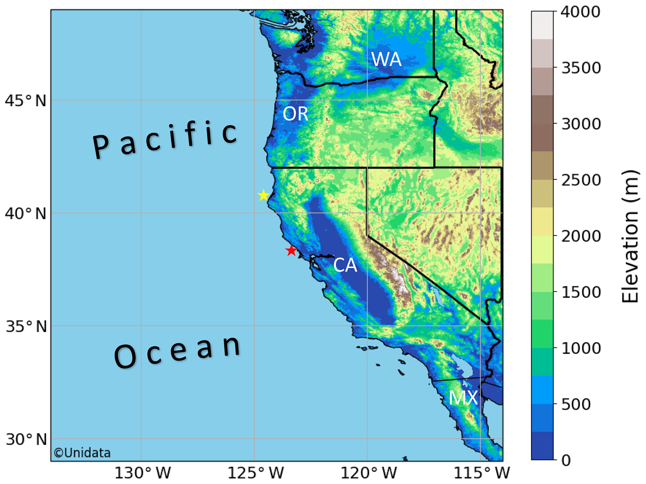
Figure 1Study region covering the western United States and the NEP for the SOM analysis. United States abbreviations WA, OR, and CA represent Washington, Oregon, and California, respectively, while MX represents Mexico. The red and yellow stars denote the locations of buoys 46013 (Bodega Bay) and 46022 (Eel River), respectively.
2.1 Pattern identification
The SOM is a type of neural network that uses a competitive, unsupervised machine learning technique (e.g., Reichstein et al., 2019) to develop a two-dimensional topology (map) of nodes that represents the n-dimensional input data. In unsupervised learning, the machine learning model is expected to reveal the structure of the input data set. Specifically in the case of training a SOM, the user is required to provide a two-dimensional input array (typically time × space), and the node topology organizes itself to mimic the input data. That is, each SOM node represents a group of similar input vectors where an input vector is a single data sample. In the case here, we provide one input vector for each time of interest.
We choose to employ the SOM technique due to its ability to group similar patterns and therefore reveal dissimilar patterns that may be hidden in the large NARR data set considered here. To this end, we use the MATLAB SOM Toolbox (version 2.1) to generate the SOM using the batch algorithm. This algorithm follows the well-known Kohonen technique (Kohonen, 1990). The SOM batch training procedure can be described as follows.
-
Define the number of nodes and iterations (one iteration is defined as a single pass through all of the input data vectors), in addition to the neighborhood radius.
-
From the data set, determine the two eigenvectors that have the largest eigenvalues; initialize the SOM node weights linearly along these eigenvectors to provide a first approximation of the input data set.
-
Present all vectors from the input data and calculate the Euclidean distance between each input vector and each node, where the Euclidean distance given two points a and b in {x,y} space.
-
Update the neighborhood radius.
-
Determine the node that most closely matches each input vector; the winning node is characterized by the minimum Euclidean distance.
-
Update the weight of each node – where the new weight is equal to the weighted average of each input data vector to which that node or any nodes in its neighborhood responded – after a single iteration.
-
Repeat steps 3–6 for n iterations.
Choosing the number of nodes is critical because a map with too few nodes yields larger sample sizes but insufficient detail, while one with too many nodes yields greater detail but insufficient sample sizes. For the present study, a series of sensitivity tests is conducted using different node map sizes to determine an optimal number of nodes (Fig. 2). Quantization and topographic errors (QE and TE, respectively) for each map are calculated. The QE, which is a measure of map resolution, is equal to the average distance between each input vector and the best matching node, while the TE indicates map topology preservation by determining the percentage of input vectors whose first and second best matching nodes are not adjacent. As the number of nodes increases, the QE decreases, typically at the cost of sacrificing node topology. This trade-off is shown quite well in Fig. 2: the QE decrease is most pronounced as the number of nodes increases from approximately 9 to 20, and the TE increase is most notable above approximately 30 nodes. Moreover, using a nonuniform (rectangular) map appears to reduce the TE, which supports previous work showing the superiority of rectangular maps over square maps (e.g., Ultsch and Herrmann, 2005). Due to the TE minimum at 20 nodes and a relatively marginal decrease in QE after 20 nodes, in addition to ample pattern detail and sufficient sample sizes, for this study we choose to use a 4×5 node map. Moreover, we choose to iterate 5000 times and use an initial neighborhood radius of 4. The neighborhood radius, which determines the number of nodes surrounding the winning node that nudge toward the input vector, slowly reduces to one (only the winning node is nudged) through the training period. Overall, our choices are similar to and follow guidelines outlined in prior SOM studies that focus on vertical sounding classification problems (e.g., Jensen et al., 2012; Nowotarski and Jensen, 2013; Stauffer et al., 2017) and synoptic meteorology pattern recognition (e.g., Cassano et al., 2015; Ford et al., 2015; Mechem et al., 2018). Additionally, we find that changing the initial parameters (iterations and neighborhood radius to 25 000 and 2, respectively) has a relatively small impact on the final node topology similar to other studies (e.g., Cassano et al., 2006; Skific et al., 2009). Once training is complete, and the node topology has organized itself to best represent the input data set, each input vector is associated with one of the map nodes.
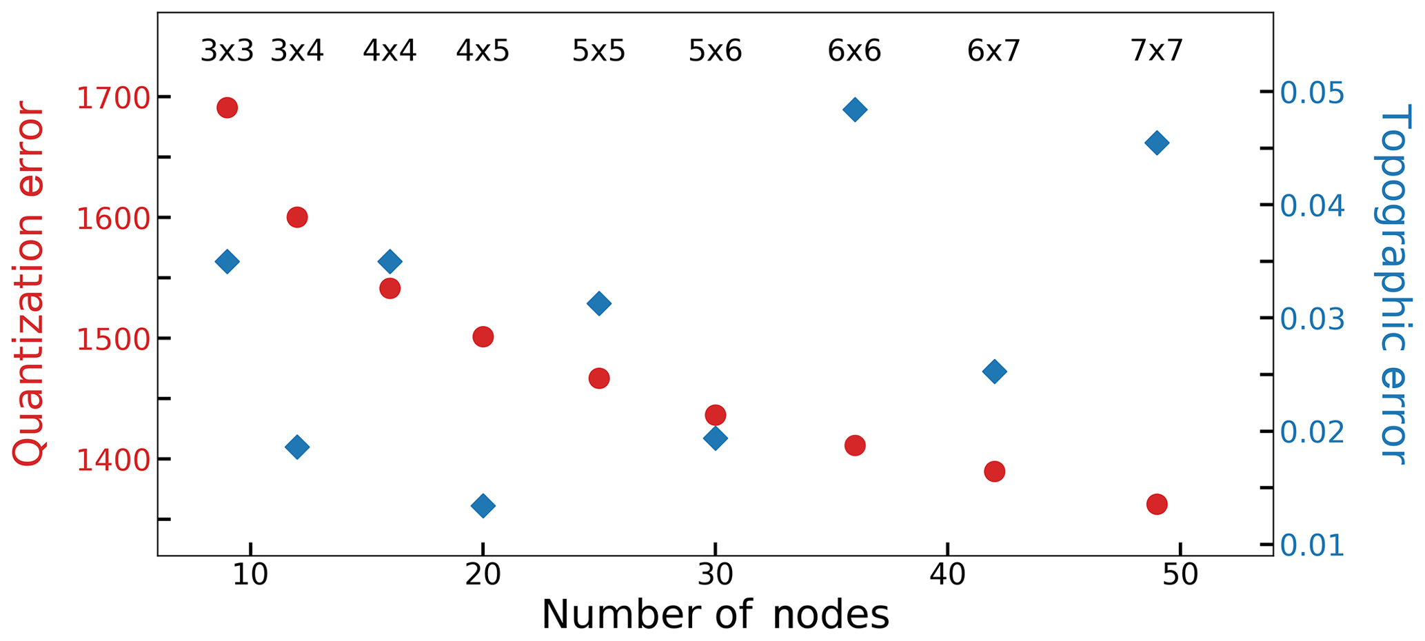
Figure 2The quantization (red circles; left axis) and topographic (blue diamonds; right axis) errors for each SOM configuration tested in this study. SOM node topologies (rows × columns) range from 3×3 to 7×7; we choose to use a 4×5 node map.
Similar to previous work (e.g., Cavazos, 2000; Tymvios et al., 2010; Mechem et al., 2018), we choose an isobaric height field as our input data. Specifically, we use the 850 hPa spatial anomaly height field because we expect this variable to most accurately represent the location and strength of the NPH. We note that we also explore using the sea-level pressure field as our input data; however, the result is an inaccurate representation of the different NPH patterns because there are many regions over the western United States where the sea-level pressure is extrapolated using a standard atmosphere assumption due to elevated terrain. While this extrapolation does also occur at 850 hPa, there are far fewer locations whose surface pressure is often lower than 850 hPa. For the two-dimensional input array, we use the 00:00 UTC NARR 32 km product for each day during the months June through September from 2004 through 2014. The use of a single time per day is permissible due to the timescale at which the pressure patterns of interest evolve and to also correspond with the satellite data. Spatial anomalies are calculated for each day by subtracting the domain-averaged 850 hPa height from the 850 hPa height at each grid point. Each row of the input array represents 1 d from our data set, while each column represents a grid box from our NARR domain. The dimensions (rows × columns) of our input array are 1342×6952. We note that our SOM results are largely insensitive to the years (excluding 2004 and 2014) and the domain size (±3 grid points (96 km) in all four directions) considered (not shown).
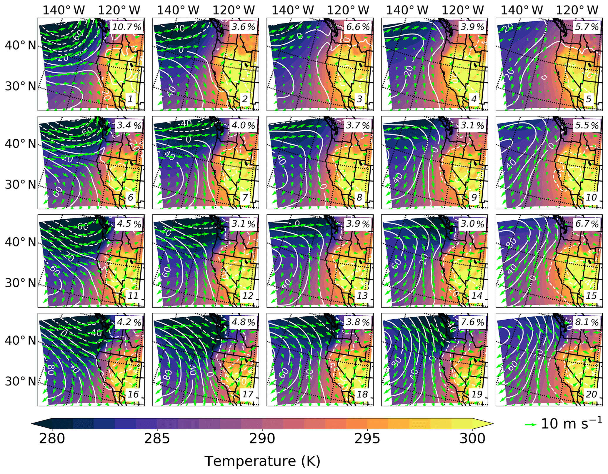
Figure 3Synoptic-scale 850 hPa spatial anomaly height field (white lines contoured every 20 m), in addition to temporal mean temperatures (contoured every 1 K according to color bar) and wind vectors (lime green arrows with 10 m s−1 reference vector) as represented by the 4×5 SOM node topology. Each panel represents a node (number displayed in the bottom right corner), while the percentage frequency of occurrence is displayed in the top right corner.
2.2 Data sets
In this study, we consider afternoon satellite measurements from Aqua MODIS because we use 00:00 UTC NARR grids to generate the SOM. The satellite images, which are typically retrieved between 20:30 and 23:30 UTC, are paired with the NARR grid for the next day. For instance, we link the MODIS retrieval from 22:00 UTC on 5 July 2010 to the NARR grid from 00:00 UTC on 6 July 2010. Even in the instance where the time difference between a MODIS image and NARR grid is a maximum (approximately 3.5 h), we expect the influence of time mismatch to be minimal because we focus on the synoptic scale over relatively short time periods. Moreover, any two consecutive images (∼5 min apart) are stitched together and counted as one sample. The MODIS files (specifically, the Level 2 MYD06 product) provide cloud information (namely, τ, re, cloud phase, cloud-top pressure, and cloud-top temperature) at 1 km horizontal spacing. We then interpolate these data to a uniform 1∕10∘ ∘ (∼10 km × 10 km) grid to be closer to the native horizontal grid spacing (∼32 km) of the NARR output without losing too much detail. We note that interpolating the MODIS data set to the NARR grid yields qualitatively and quantitatively similar results: differences in the summary statistics shown in Table 2 are typically less than 5 % (not shown).
2.3 MODIS processing
For the MODIS retrievals, values of re and τ are calculated utilizing a bispectral solar reflectance method (Nakajima and King, 1990), whereby reflectance information is gleaned at 0.75 and 3.7 µm. We choose to interrogate retrievals from the 3.7 µm channel because these data best represent the actual value of re at cloud top (Platnick, 2000; Rausch et al., 2017). Cloud liquid water path (LWP) may then be inferred from the re and τ retrievals by the equation LWP=Cρlreτ, where C is a function of the assumed vertical distribution of cloud liquid water, and ρl is the density of liquid water (e.g., Miller et al., 2016). For the calculation of LWP, we assume that the cloud vertical profile is approximately adiabatic (; e.g., Wood and Hartmann, 2006) and that N is approximately constant with height. Values of N may be estimated from observations of τ and re after assuming an adiabatic cloud model (Bennartz, 2007), similar to the method used in Juliano et al. (2019b). Moreover, we estimate fractional cloud albedo (αc) using MODIS retrievals of τ and following Lacis and Hansen (1974): , where τ is optical thickness. The top of the atmosphere CRESW may then be calculated as CRE, where So is the solar constant (1370 W m−2) and αo is the ocean albedo [0.10 (10 %)]. The MODIS processing techniques are expounded in Juliano et al. (2019b).
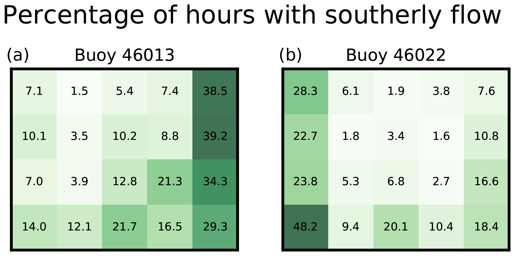
Figure 4Percentage of southerly flow hours recorded at each buoy site along the California coastline for each node in the 4×5 SOM topology: (a) buoy 46013 (Bodega Bay; 38.238∘ N, 123.307∘ W) and (b) buoy 46022 (Eel River; 40.712∘ N, 124.529∘ W).
3.1 Synoptic meteorological conditions
We now use the SOM output to investigate the various NARR 850 hPa meteorological patterns that are present during boreal summer over the NEP from 2004 to 2014 (Fig. 3). There are several key features to discuss. The leftmost part of the map (nodes 1, 6, 11, and 16) represents a regime where the NPH is relatively suppressed and a land-falling low-pressure system is dominant. In general, strong, onshore flow is noticeable, and the flow diverges near the coastline. Relatively low temperatures related to the cyclonic circulation are present across the domain over the ocean and close to the shoreline over land. Combined, these patterns account for approximately 22.8 % of days in the data set. Moving from left to right across the map, there is a smooth transition between patterns, and the presence of the NPH becomes more noticeable. The rightmost portion of the map (nodes 5, 10, 15, and 20) represents a regime where the NPH is dominant, and the nearshore 850 hPa flow is relatively weak or even directed offshore. Interestingly, there is a cyclonic circulation centered around 36∘ N, 127∘ W in node 5. For all of these nodes, especially node 5, relatively high temperatures are observed along the coastline in the northern portion of the domain. Approximately 26.0 % of all days in the data set fall under these four nodes with a dominant NPH. Overall, during the warm season months over the NEP, the SOM reveals two pronounced regimes – the dominant NPH and the land-falling cyclone – and in between a spectrum of large-scale meteorological conditions.
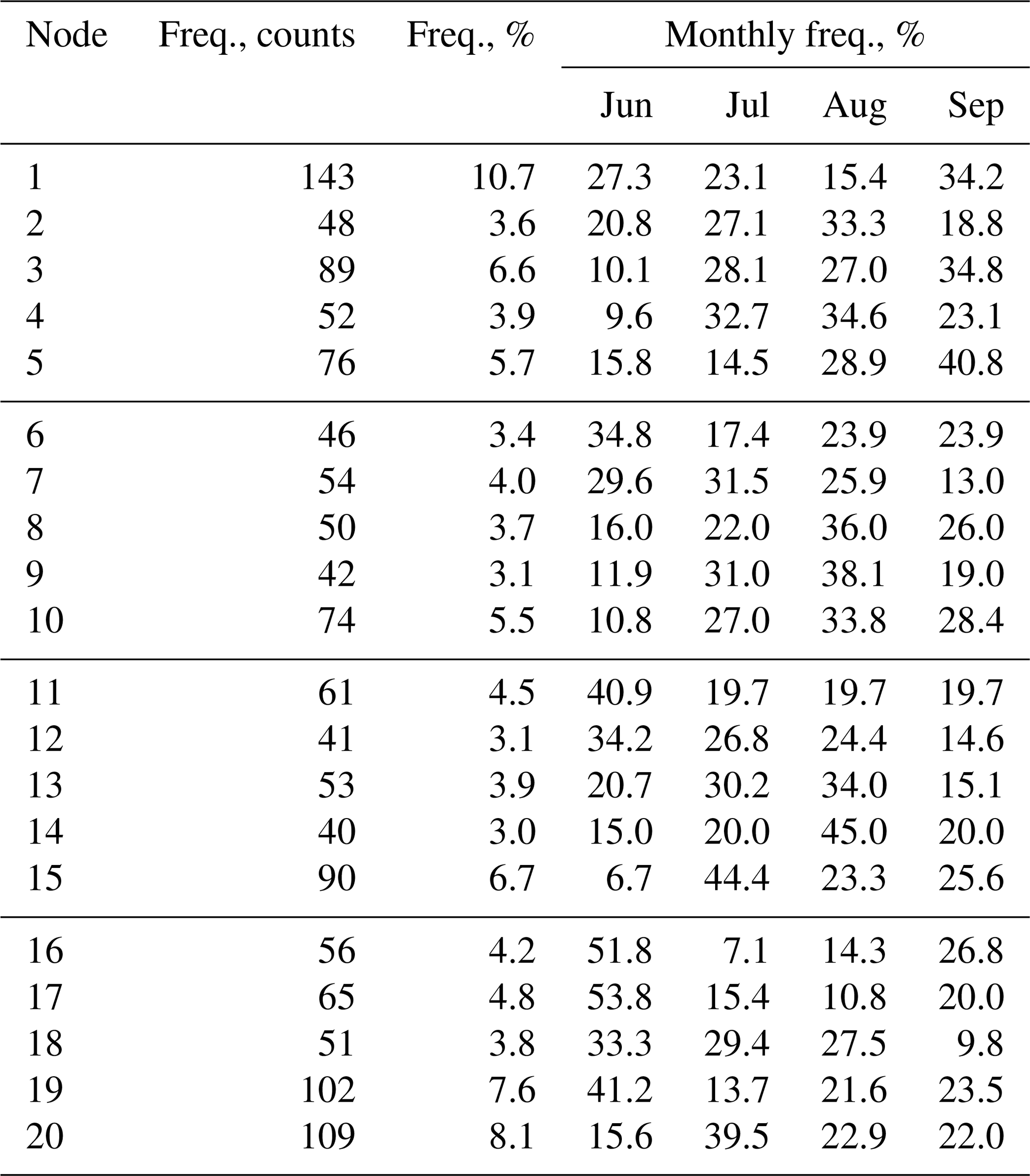
Table 1Summary statistics for SOM node frequency. Total and monthly frequencies over the 11-year period are shown.
Large-scale regimes associated with both offshore continental flow driven by the NPH (e.g., node 5) and onshore continental flow driven by a land-falling cyclone (e.g., node 16) at 850 hPa often cause the near-surface alongshore flow to become southerly along the California coastline, as depicted by the observations from buoys 46013 and 46022 (Fig. 4; see Fig. 1). Offshore flow generates a weakening or reversal in the alongshore pressure gradient that drives southerly flow, while onshore flow is blocked by the coastal terrain, thereby forcing the flow to diverge in the meridional direction. The location and intensity of the NPH are main factors in dictating the northward extent and strength of the southerly flow for the 850 hPa offshore flow events. Similarly, the location and intensity of a land-falling cyclone control the location of alongshore flow bifurcation.
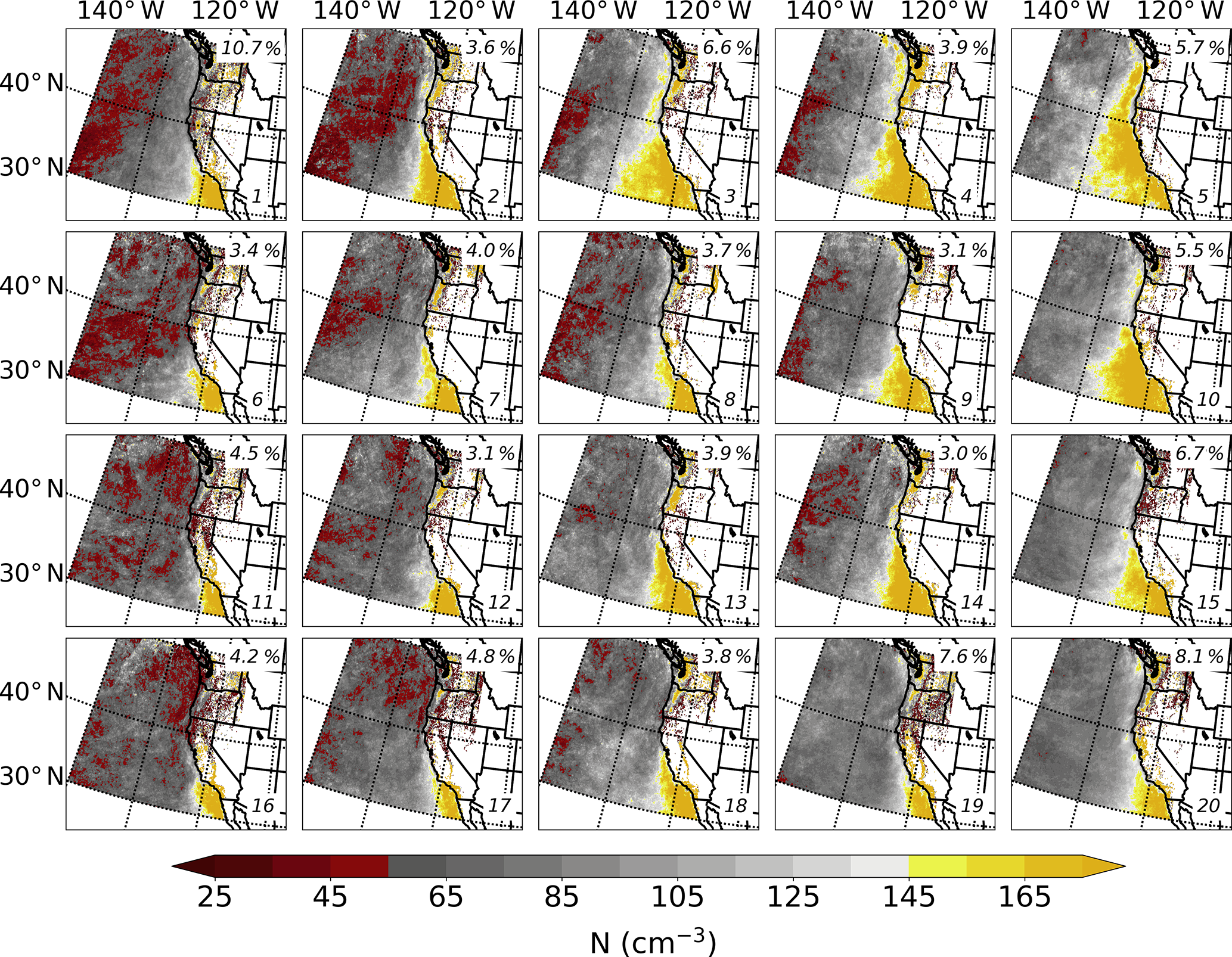
Figure 5MODIS estimation of N (contoured every 10 cm−3 according to the color bar) for each node in the 4×5 SOM topology. Each panel represents the mean conditions for each node (number displayed in the bottom right corner), while the percentage frequency of occurrence is displayed in the top right corner.
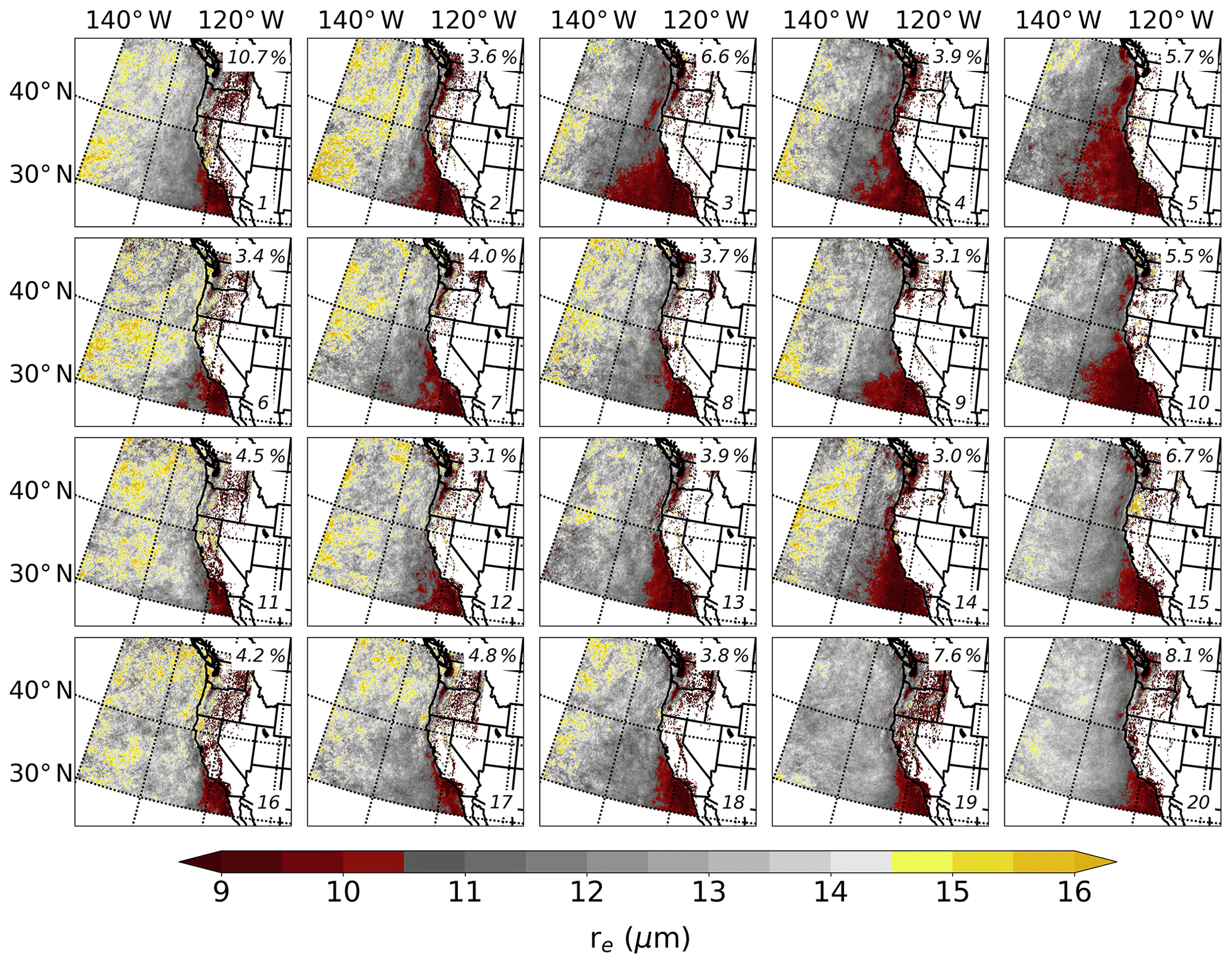
Figure 6As in Fig. 5 except for the MODIS retrieval of re (contoured every 0.5 µm according to the color bar).
Measurements from buoy 46013 (Bodega Bay), which is located just northwest of Point Reyes, California, suggest that southerly flow is present for a substantial number of hours (∼38.5 %, ∼39.2 %, ∼34.3 %, and ∼29.3 %) that fall within nodes 5, 10, 15, and 20, respectively. Meanwhile, buoy observations just northwest of Cape Mendocino (buoy 46022, Eel River) show strong influence from the land-falling cyclone (onshore flow) patterns; ∼28.3 %, ∼22.7 %, ∼23.8 %, and ∼48.2 % of the hours for nodes 1, 6, and 11, and 16, respectively, are characterized by southerly flow. The dependence of these regional flow conditions on the synoptic-scale forcing is important for various meteorological applications, such as ocean upwelling and offshore wind energy forecasting.
Table 1 lists the total and monthly frequencies of occurrence for each node. In general, the majority of days that are represented by the land-falling cyclone regime (nodes 1, 6, 11, and 16) are in early summer (June) and early fall (September). This is not surprising because these systems are more common during transition seasons than during summer (e.g., Reitan, 1974). Additionally, we find that the dominant NPH regime (nodes 5, 10, 15, and 20) occurs most often in July, August, or September. We also note that node 5, which features a weak regional height gradient, shows a strong increase in frequency of occurrence over time (frequencies of 15.8 %, 14.5 %, 28.9 %, and 40.8 % in June, July, August, and September, respectively).
Due to the nature of the SOM, adjacent synoptic-scale patterns are similar to one another, and there is a gradual transition between the nodes as one moves across the SOM. The SOM patterns farther left on the map are associated with generally strong westerly flow offshore and divergent flow near the coastline due to a dominant cold-core land-falling cyclone. Conversely, those patterns toward the right feature northerly, and even northeasterly, flow offshore due to a dominant warm-core NPH. Moreover, several of the nodes (3, 4, and 5) feature a noticeably weak 850 hPa height gradient; on average, the winds over the ocean at this level are <5 m s−1. In general, the top right SOM nodes feature the most notable offshore continental flow (and associated weak nearshore winds at southern latitudes in the domain) because the 850 hPa height contours are oriented northeast–southwest and the wind vectors have pronounced south and west components. Therefore, one might expect to see relatively high N and small re values dominate in these nodes because they appear to be influenced strongly by continental air masses.
3.2 MODIS cloud retrievals
Figures 5 and 6 show the mean N and re values from MODIS that are associated with each node. In Fig. 5, the red (yellow) end of the color bar corresponds to relatively low (high) N, and in Fig. 6 the red (yellow) end of the color bar corresponds to relatively small (large) re. Therefore, yellow regions in Fig. 5 and red regions in Fig. 6 indicate a potential influence of continental and/or shipping aerosol sources on marine clouds.
Although the MODIS retrievals are not used directly to generate the SOM, and instead are simply associated with the corresponding days in each node, there is an apparent connection between the various synoptic-scale patterns in the 850 hPa height fields (which are used to generate the SOM) depicted in Fig. 3 and the MODIS cloud properties shown in Figs. 5 and 6. Generally, there are more regions of high N and smaller re as one moves from left to right across the SOM; that is, nodes to the left (right) on the SOM represent days where marine clouds are, on average, composed of less numerous and larger (more numerous and smaller) cloud droplets. Through a visual inspection, node 5 appears to be most representative of cases where marine stratiform clouds have more numerous and smaller droplets. As shown in the analysis in Fig. 3, node 5 is characterized by distinct offshore continental flow at 850 hPa, in addition to very weak northerly or southerly flow near the shoreline. These results highlight the utility of using reanalysis to define modes of large-scale pressure patterns and subsequently incorporate other data sets – satellite observations in the case here – to understand interactions across spatial scales that could not otherwise be gleaned from the original reanalysis products themselves.

Figure 7Frequency distributions of re (µm; colored magenta), N (cm−3; colored dark blue), and CRESW (W m−2; colored light green) for each node over the ocean in the 4×5 SOM topology. The node number is shown in the top right corner of each subplot. The actual distributions are shown for node 16, while the difference relative to node 16 (node x minus node 16, where x is a given node) is shown for all other nodes. Therefore, smaller (larger) values indicate a deficit (surplus) relative to node 16. The distributions of re and N are generated from the plan views in Figs. 4 and 5. The distribution of CRESW is calculated from the plan view of τ (see Sect. 2.3), which is generated similarly to re and N but is not shown here. Also, median values of each distribution are documented in Table 2.
Evident in all of the SOM nodes is a region of high N and small re south of the pronounced coastal bend near Point Conception, California (approximately 34.4∘ N, 120.5∘ W). This nearshore oceanic region is likely polluted due to its proximity to population centers (namely Los Angeles, California; San Diego, California; and Tijuana, Mexico) and wildfire activity (e.g., Duong et al., 2011; Metcalf et al., 2012; Zauscher et al., 2013). Also, this area serves as a major port for international trade and hosts numerous refineries (e.g., Ault et al., 2009; Ryerson et al., 2013). In this region, transport of aerosol is governed typically by the synoptic-scale conditions and mesoscale land–sea breeze processes (e.g., Agel et al., 2011; Naifang et al., 2013); however, previous work suggests that the pervasive Catalina Eddy – a phenomenon linked to the generation of CTDs (e.g., Skamarock et al., 2002) – may transport pollution offshore and toward the north (Wakimoto, 1987). We hypothesize that the MODIS retrievals presented here show clearly that the first aerosol indirect effect (Twomey, 1977) is more pronounced in the nodes farther to the right on the map due to this complex combination of atmospheric processes that impacts marine clouds through aerosol–cloud interactions. Specifically, we hypothesize that the transport of continental aerosol (e.g., nitrates, sulfates, biogenic organics, and dust) into the marine environment, in addition to the interaction of ship track aerosol (e.g., sulfates) and marine aerosol (e.g., sea salt), increases the number of cloud condensation nuclei (CCN) and therefore cloud droplets. While we do not test these hypotheses here, we recommend that future studies examine them using, for example, backward trajectories – similar to previous studies that consider individual cases (e.g., Painemal et al., 2015; Albrecht et al., 2019; Juliano et al., 2019a, b) – in combination with numerical simulations that explicitly treat aerosol. These potential aerosol–cloud interactions are most notable within several hundred kilometers of the western United States and Baja California coastlines; however, remote oceanic locations also appear to be influenced strongly by the NPH regime. Additionally, the areas likely affected by pollution sources extend along nearly the entire coastline in the nodes to the right on the SOM, while the nodes to the left on the SOM show a much more confined region of polluted clouds due to strong onshore flow. In general, the nodes display varying extensions according to the synoptic-scale circulation pattern.
Frequency distributions reveal that between the various SOM nodes, cloud micro- and macrophysical properties exhibit a broad range that is dependent on the prevailing synoptic-scale pattern (Fig. 7; see Table 2 for median values). The distributions confirm that node 5, in addition to nodes 3, 4, and 10, represents the scenarios where MBL clouds are characterized by relatively high N and small re compared to the other meteorological nodes. The median values of N and re are 95.5 cm−3 and 10.3 µm for node 3, 91.0 cm−3 and 10.9 µm for node 4, 103.7 cm−3 and 10.0 µm for node 5, and 94.8 cm−3 and 10.5 µm for node 10. For most of the other nodes, the frequency distributions of N and re are shifted toward the left and right, respectively, indicative of fewer and larger cloud droplets. In the patterns that are much different than nodes 3, 4, 5, and 10 – for example, node 16, in addition to nodes 6, 11, and 12 – the distributions are shifted appreciably such that the median values of N and re are 56.1 cm−3 and 12.3 µm for node 6, 55.1 cm−3 and 12.5 µm for node 11, 62.6 cm−3 and 12.2 µm for node 12, and 57.3 cm−3 and 12.3 µm for node 16.
Table 2Summary statistics for SOM node meteorological and cloud properties. We tabulate median values of the frequency distributions of re, N, CRESW (see Fig. 7), LWP, and H as well as those of meteorological variables LCF, LTS, and qv. Distributions are calculated over the oceanic area shown in Figs. 3, 5, and 6.
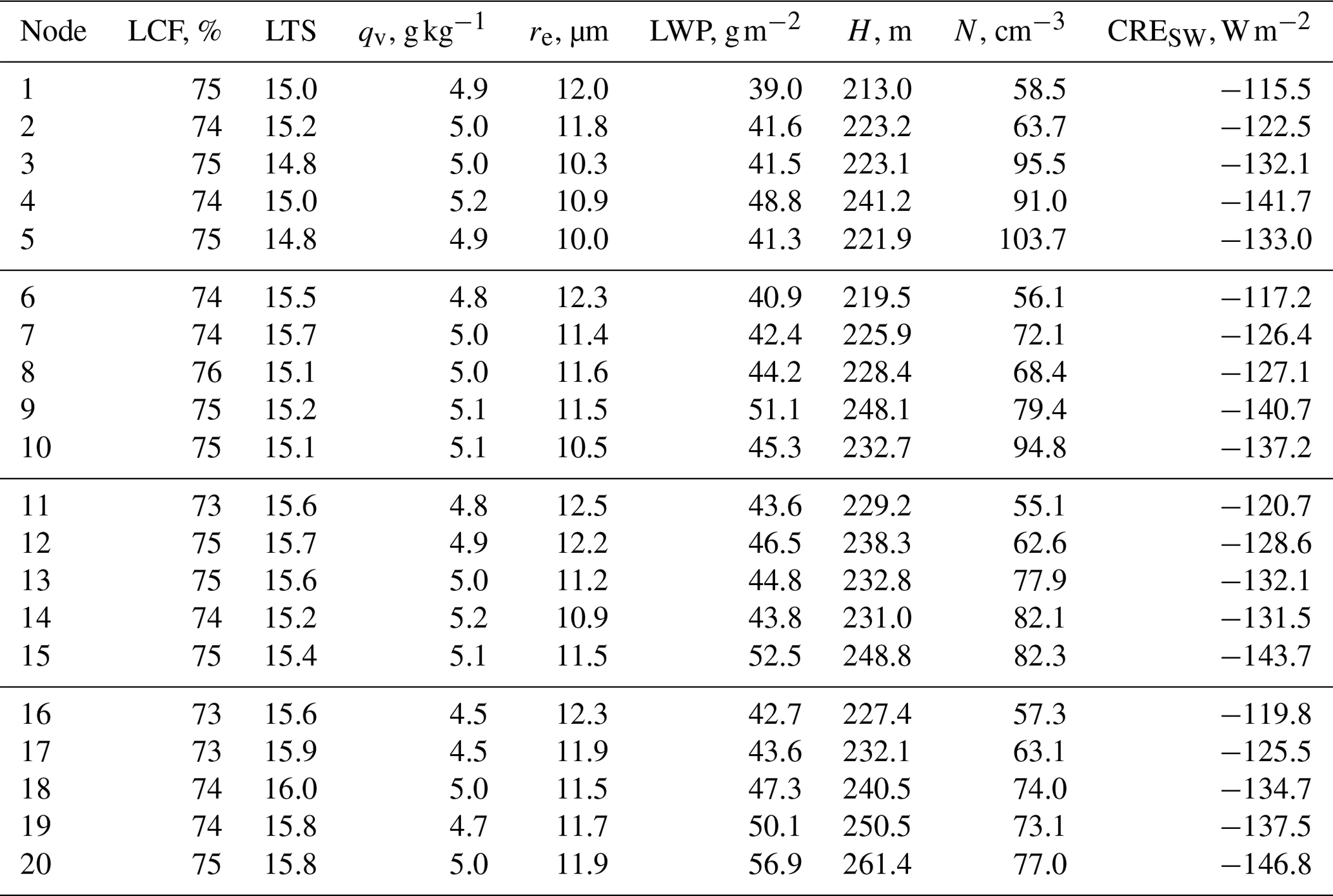
To explore the potential impact of the regional meteorology associated with each of the synoptic-scale patterns – compared to simply the abundance of aerosol – on the observed cloud properties, we also examine low cloud fraction (LCF), lower tropospheric stability (LTS; Klein and Hartmann, 1993), and 850–700 hPa mean water vapor mixing ratio (qv) from the NARR grids (Table 2). In general, LCF increases, LTS decreases, and qv increases from left to right across the SOM; however, these meteorological variables do not show much variability among the different nodes. MODIS retrievals of LWP and cloud depth (H), which are macrophysical quantities that may serve as indicators of meteorological forcing, show a weak trend of increasing values as one moves from left to right across the map; however, there is large spread in LWP and H between the NPH regime patterns. To further investigate the relative influences of meteorological versus aerosol forcings on the satellite-retrieved cloud microphysical and radiative properties, we examine various susceptibility relationships following Platnick and Twomey (1994).
Table 3Susceptibility parameters calculated for each node. Here we use the same data that are used to calculate the values in Table 2; that is, the susceptibility for each node is based on the linear regression of all spatial points located within the oceanic area shown in Figs. 3, 5, and 6 and of all MODIS retrieval times associated with that node.
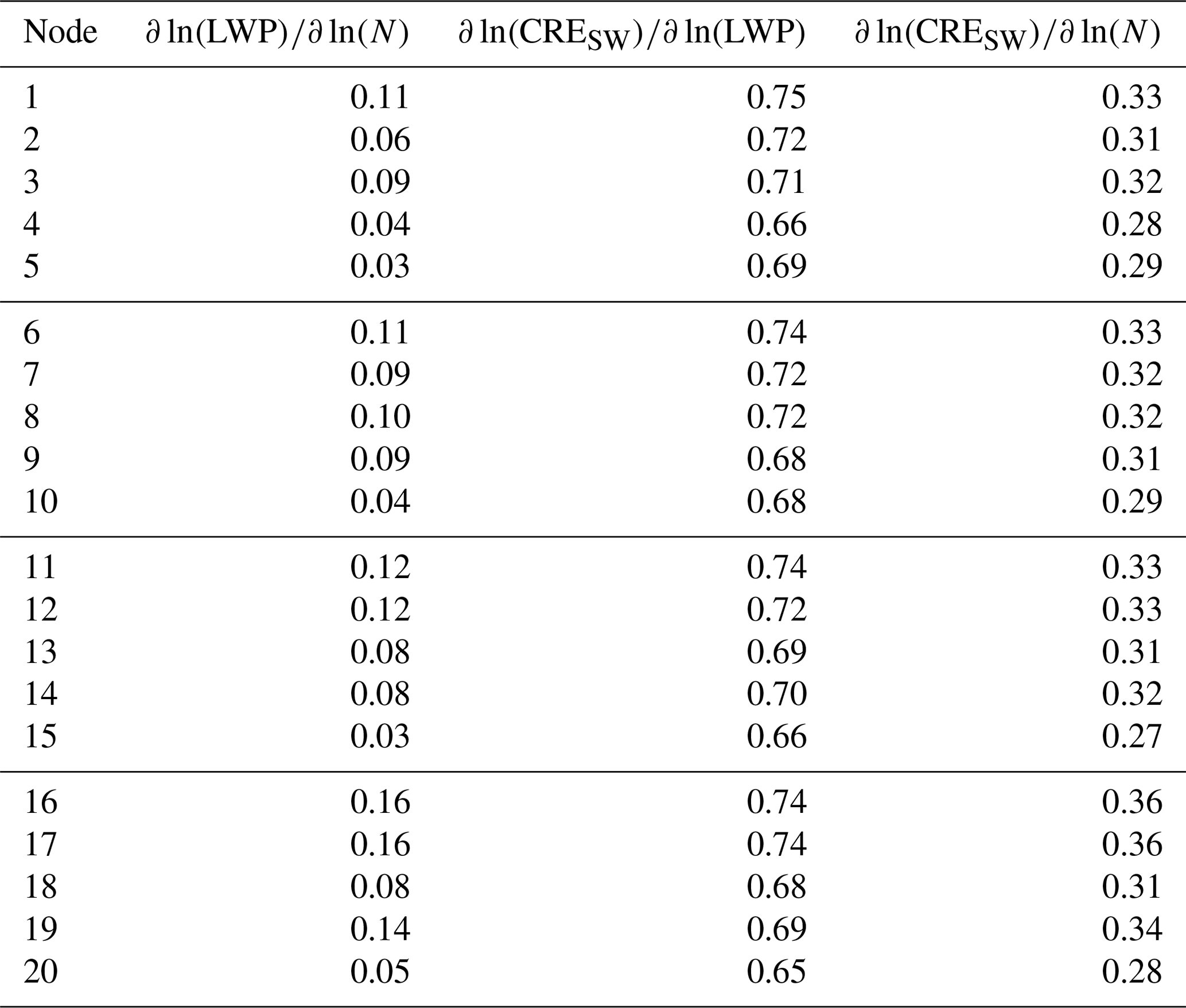
For this susceptibility analysis, we consider the MODIS variables N, LWP, and CRESW. Using these three variables, we calculate three susceptibility parameters: , , and (Table 3). The latter two relationships represent the meteorological and aerosol forcings, respectively, on the shortwave CRE. In general, susceptibility decreases from left to right on the node map, as one moves from the land-falling cyclone regime to the dominant NPH regime, e.g., from node 16 to node 12 to node 8 to node 5. The strong susceptibility signal represented by the relationship (values ranging from 0.65 to 0.75) suggests that changes in CRESW are strongly and positively related to changes in LWP, which is likely mainly due to meteorological forcing, as the relationship is relatively weak (values ranging from 0.03 to 0.16). While in all of the nodes the meteorological forcing does dominate over the aerosol forcing in the context of CRESW, we point out that the magnitude of the aerosol forcing on shortwave cloud radiative properties, represented by , ranges from approximately 40 % to 49 % of the meteorological forcing depending on the large-scale circulation pattern.
In Fig. 8, we summarize the relationship between N, LWP, and CRESW. In the large-scale circulation patterns where the NPH is relatively suppressed and onshore flow dominates due to a land-falling cyclone (nodes 1, 6, 11, and 16), N is relatively small (ranging from 55.1 and 58.5 cm−3) and LWP is relatively low (39.0 to 43.6 g m−2), corresponding to relatively weak CRESW (−120.7 to −115.5 W m−2). For the circulation patterns where the NPH is controlling the synoptic-scale setup (nodes 5, 10, 15, 20), while N is relatively large, LWP is relatively high, and CRESW is relatively strong compared to the land-falling cyclone; however, these three variables exhibit much larger spread within the NPH regime compared to within the land-falling cyclone regime. For instance, median values for N, LWP, and CRESW are 103.7 cm−3, 41.3 g m−2, and −133.0 W m−2 for node 5 and 77.0 cm−3, 56.9 g m−2, and −146.8 W m−2 for node 20. Moreover, we again highlight the importance of both meteorology and aerosol for cloud properties: positive changes in LWP of ∼19 % and N of ∼7 % from node 1 to node 5 lead to +11 % more reflective clouds, and positive changes in LWP of ∼6 % and N of ∼77 % from node 1 to node 5 lead to +15 % more reflective clouds. Our results suggest that both the meteorological and aerosol forcings are first-order effects that cannot be neglected when examining the influence of large-scale circulation patterns on MBL cloud properties over the NEP.
We emphasize that Fig. 8 elucidates the large range in LWP for the NPH regime, which is in stark contrast to the relatively narrow range in LWP for the land-falling cyclone regime. As a result, for low LWP, the transition from the land-falling cyclone to NPH regime results in little to no change in LWP but a drastic increase in N and a commensurate increase in CRESW; this indicates that the meteorology exhibits little control on CRESW in the low-LWP NPH regime, and instead it is predominately driven by changes in N, which we relate to the offshore transport of continental aerosol. On the contrary, when moving from the land-falling cyclone regime to the high-LWP NPH regime, there is an increase in LWP as well as N, indicating the role of both factors in CRESW, as discussed above.
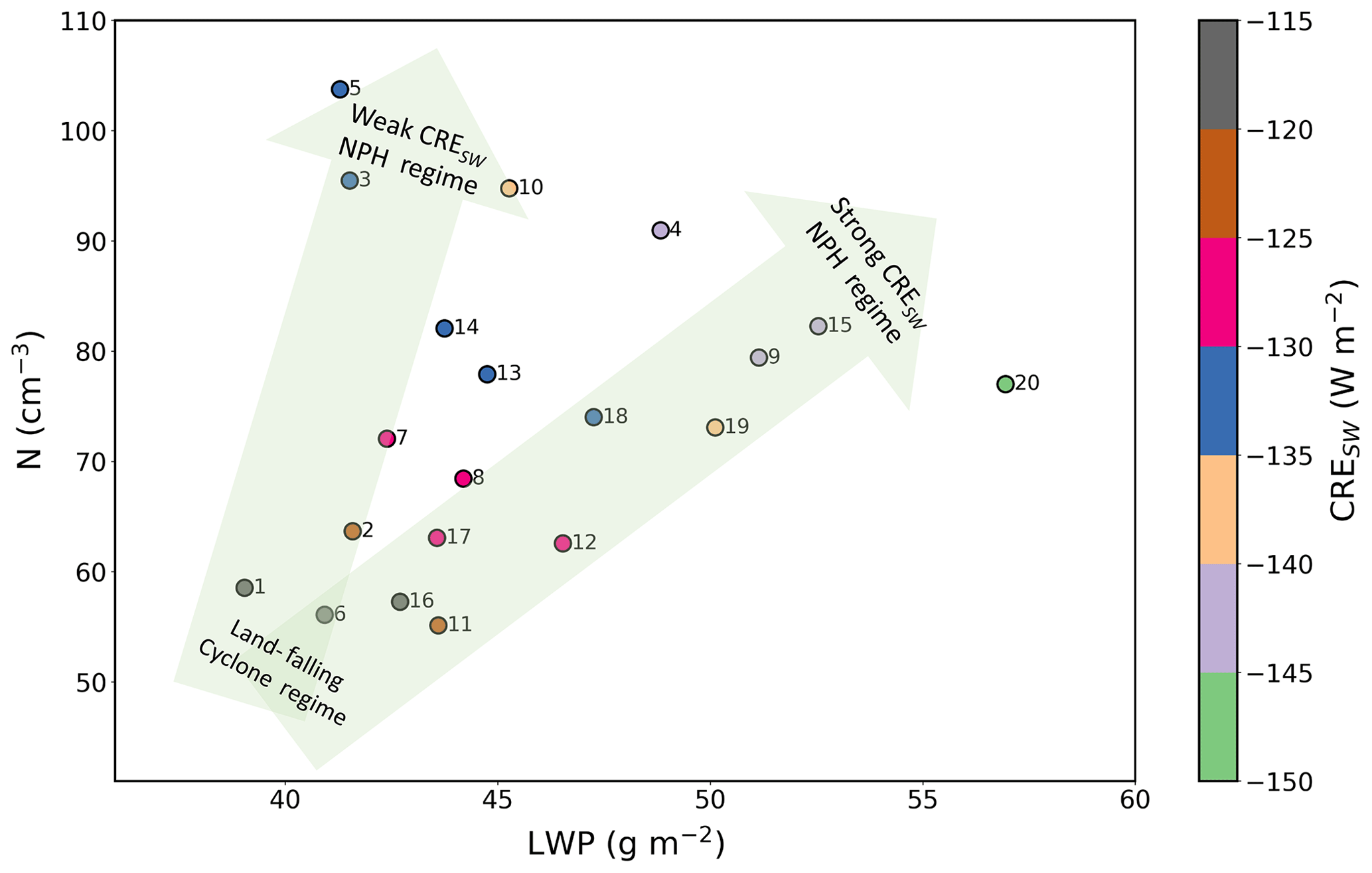
Figure 8Scatter plot of LWP versus N, colored by CRESW for each of the nodes. Each value represents the median, and values are taken from Table 2.
Overall, our SOM results elucidate the apparent coupling between NPH dynamics and mesoscale MBL cloud properties through both meteorological and aerosol effects. In terms of the impact of large-scale circulation on cloud physics through aerosol forcing, generally weak flow and/or an enhancement in offshore continental flow at 850 hPa (e.g., node 5) likely augments aerosol transport into the marine layer, thereby increasing both the number of CCN and the brightness (reflection) of MBL clouds. Moreover, we hypothesize that a weaker regional pressure gradient allows for the transport of aerosol by the coastal jet due to the dominance of localized land–sea breeze circulations, which may advect continental aerosol offshore (e.g., Lawrence and Lelieveld, 2010; Loughner et al., 2014; Mazzuca et al., 2017). In contrast, a suppression in offshore continental flow (e.g., node 16) likely inhibits continental aerosol transport into the marine layer, thereby decreasing both the number of CCN and the brightness (reflection) of MBL clouds. We note that other factors not explicitly accounted for here, such as aerosol composition, turbulence, and sea surface temperature, may also play an important role in the linkage between large-scale meteorology and low-cloud properties.
Through the use of a SOM, we show that the location and intensity of the NPH, as well as the presence of land-falling low-pressure systems, play a role in modifying MBL cloud micro- and macrophysical properties offshore of the western United States during boreal summer. The 850 hPa height field is chosen as the meteorological input variable for the SOM algorithm because it represents the large-scale circulation over the NEP well. Results from the SOM, using an 11-year period of NARR data, reveal several distinct synoptic patterns present over the NEP during the warm season as well as their frequencies of occurrence; however, most notable is the high frequency of pronounced offshore continental flow and generally weak flow. Incorporating MODIS observations into the analysis yields a connection between the synoptic-scale dynamics and mesoscale cloud properties. That is, combining the SOM approach with the satellite retrievals reveals that synoptic-scale circulation patterns modify both the regional meteorology and aerosol transport. Specifically, the land-falling cyclone regime is characterized by relatively low N, small LWP, and weak CRESW. In comparison, the NPH regime generally shows relatively high N, large LWP, and strong CRESW, albeit these variables exhibit much larger spread compared with those of the land-falling cyclone regime. In the middle of the SOM, the circulation patterns exhibit a smooth transition between these two regimes in terms of both the meteorological setup and MBL cloud properties.
The findings reported here may be of significant interest to atmospheric science communities utilizing climate models (CMs) because the synoptic-scale flow–cloud microphysics relationships from the SOM may be used to test CMs and probe uncertainties in their simulation of aerosol effects. For instance, the SOM results may be used to better understand if CMs are capable of reproducing similar patterns between large-scale circulation and cloud microphysical/radiative effects. One could then quantify the impact of using the radiative effect from the observed SOM relationship with the modeled 850 hPa height field rather than the model-predicted radiative effect over the semi-permanent marine stratiform regions. Also, this analysis could be extended to evaluate in a statistical sense the ability of long-term simulations to replicate each large-scale pattern.
Moreover, most CMs have difficulty with accurately representing MBL clouds – which are susceptible to aerosol effects – because they often use a horizontal grid spacing that is too large (≳10 km). However, reproducing large-scale meteorological fields, such as pressure or isobaric height, is typically easier for CMs. Here, we demonstrate a “proof-of-concept” study of a novel method to link well-resolved synoptic-scale features to cloud microphysics and the shortwave radiative effect. Because the approach is relatively simple to implement, it may be applied to other problems in atmospheric science involving interactions between spatial scales.
While the results presented here are promising, a data set spanning a longer time period is required to develop a robust analysis that evaluates the ability of CMs to reproduce the observed synoptic-scale weather patterns and mesoscale cloud properties. In general, using machine learning techniques to connect large-scale circulation patterns to cloud microphysics, which is challenging using solely observations from field campaigns or modeling case studies, is important for accurate predictions of future atmospheric climate. The results presented here may not be applicable to all marine stratiform cloud decks owing to potential differences in the frequency, strength, and location of the respective high-pressure circulation, as well as differences in, for example, coastal geometry and topography, continental land use, aerosol sources, and sea surface temperature. Future work will explore the application of the methodology outlined herein to the other dominant MBL cloud regions of the world using global reanalysis products and model output.
NARR reanalysis is available from the National Oceanic and Atmospheric Administration (NOAA) National Centers for Environmental Information (NCEI) website (https://www.ncdc.noaa.gov/, last access: 17 March 2020), Aqua MODIS Level 2 satellite retrievals are available from the National Aeronautics and Space Administration (NASA) Earthdata website (https://search.earthdata.nasa.gov/, last access: 17 March 2020), and buoy observations are available from the NOAA National Data Buoy Center (NDBC) website (https://www.ndbc.noaa.gov/, last access: 17 March 2020). The MATLAB SOM Toolbox code is available for download courtesy of the Helsinki University of Technology (http://www.cis.hut.fi/projects/somtoolbox/, last access: 17 March 2020). Additional codes are available upon request.
TWJ designed the study, developed the code, performed the analysis, and wrote the manuscript. ZJL made substantial contributions to the analysis and revised the manuscript.
The authors declare that they have no conflict of interest.
Timothy W. Juliano is grateful for support from the state of Wyoming, the Carlton R. Barkhurst Fellowship, and NCAR through the National Science Foundation. We would also like to acknowledge high-performance computing support from Cheyenne (https://doi.org/10.5065/D6RX99HX) provided by NCAR's Computational and Information Systems Laboratory and sponsored by the National Science Foundation. The authors thank Hugh Morrison, Andrew Gettelman, Kevin Reed, and Stefan Rahimi for providing valuable comments on an earlier version of the manuscript.
This research has been supported by the U.S. Department of Energy, Office of Science (grant no. DE-SC0016354).
This paper was edited by Philip Stier and reviewed by Johannes Mülmenstädt and one anonymous referee.
Agel, L., Lopez, V., Barlow, M., and Colby, F.: Regional and large-scale influences on summer ozone levels in Southern California, J. Appl. Meteor. Clim., 50, 800–805, 2011. a
Albrecht, B., Ghate, V., Mohrmann, J., Wood, R., Zuidema, P., Bretherton, C., Schwartz, C., Eloranta, E., Glienke, S., Donaher, S., Sarkar, M., McGibbon, J., Nugent, A. D., Shaw, R. A., Fugal, J., Minnis, P., Paliknoda, R., Lussier, L., Jensen, J., Vivekanandan, J., Ellis, S., Tsai, P., Rilling, R., Haggerty, J., Campos, T., Stell, M., Reeves, M., Beaton, S., Allison, J., Stossmeister, G., Hall, S., and Schmidt, S.: Following the Evolution of Boundary Layer Cloud Systems with the NSF–NCAR GV, B. Am. Meteorol. Soc., 100, 93–121, 2019. a
Ault, A. P., Moore, M. J., Furutani, H., and Prather, K. A.: Impact of emissions from the Los Angeles Port region on San Diego air quality during regional transport events, Environ. Sci. Technol., 43, 3500–3506, 2009. a
Bachiochi, D. R. and Krishnamurti, T. N.: Enhanced low-level stratus in the FSU coupled ocean–atmosphere model, Mon. Weather Rev., 128, 3083–3103, 2000. a
Bender, F. A., Engström, A., and Karlsson, J.: Factors Controlling Cloud Albedo in Marine Subtropical Stratocumulus Regions in Climate Models and Satellite Observations, J. Climate, 29, 3559–3587, 2016. a
Bender, F. A., Frey, L., McCoy, D. T., Grosvenor, D. P., and Mohrmann, J. K.: Assessment of aerosol–cloud–radiation correlations in satellite observations, climate models and reanalysis, Clim. Dynam., 52, 4371–4392, 2018. a
Bennartz, R.: Global assessment of marine boundary layer cloud droplet number concentration from satellite, J. Geophys. Res., 112, D02201, https://doi.org/10.1029/2006JD007547, 2007. a
Bony, S. and Dufresne, J.-L.: Marine boundary layer clouds at the heart of tropical cloud feedback uncertainties in climate models, Geophys. Res. Lett., 32, l20806, https://doi.org/10.1029/2005GL023851, 2005. a
Brient, F., Roehrig, R., and Voldoire, A.: Evaluating marine stratocumulus clouds in the CNRM‐CM6‐1 model using short‐term hindcasts, J. Adv. Model. Earth Syst., 11, 127–148, 2019. a
Cassano, E. N., Lynch, A. H., Cassano, J. J., and Koslow, M. R.: Classification of synoptic patterns in the western Arctic associated with extreme events at Barrow, Alaska, USA, Clim. Res., 30, 83–97, 2006. a
Cassano, E. N., Glisan, J. M., Cassano, J. J., Gutowski Jr., W. J., and Seefeldt, M. W.: Self-organizing map analysis of widespread temperature extremes in Alaska and Canada, Clim. Res., 62, 199–218, 2015. a
Cavazos, T.: Using self-organizing maps to investigate extreme climate events: An application to wintertime precipitation in the Balkans, J. Climate, 13, 1718–1732, 2000. a
Crosbie, E., Wang, Z., Sorooshian, A., Chuang, P. Y., Craven, J. S., Coggon, M. M., Brunke, M., Zeng, X., Jonsson, H., Woods, R. K., Flagan, R. C., and Seinfeld, J.: Stratocumulus cloud clearings and notable thermodynamic and aerosol contrasts across the clear–cloudy interface, J. Atmos. Sci., 73, 1083–1099, 2016. a
Delecluse, P., Davey, M. K., Kitamura, Y., Philander, S. G. H., Suarez, M., and Bengtsson, L.: Coupled general circulation modeling of the tropical Pacific, J. Geophys. Res., 103, 14357–14373, 1998. a
Duong, H. T., Sorooshian, A., Craven, J. S., Hersey, S. P., Metcalf, A. R., Zhang, X., Weber, R. J., Jonsson, H., Flagan, R. C., and Seinfeld, J. H.: Water-soluble organic aerosol in the Los Angeles Basin and outflow regions: Airborne and ground measurements during the 2010 CalNex field campaign, J. Geophys. Res., 116, D00V04, https://doi.org/10.1029/2011JD016674, 2011. a
Fewings, M. R., Washburn, L., Dorman, C. E., Gotschalk, C., and Lombardo, K.: Synoptic forcing of wind relaxations at Pt. Conception, California, J. Geophys. Res.-Oceans, 121, 5711–5730, 2016. a
Ford, T. W., Quiring, S. M., Frauenfeld, O. W., and Rapp, A. D.: Synoptic conditions related to soil moisture-atmosphere interactions and unorganized convection in Oklahoma, J. Geophys. Res.-Atmos., 120, 11519–11535, 2015. a
Hartmann, D. L., Ockert-Bell, M. E., and Michelsen, M. L.: The effect of cloud type on Earth's energy balance: Global analysis, J. Climate, 5, 1281–1304, 1992. a
Jensen, A. A., Thompson, A. M., and Schmidlin, F. J.: Classification of Ascension Island and Natal ozonesondes using self-organizing maps, J. Geophys. Res., 11, D04302, https://doi.org/10.1029/2011JD016573, 2012. a
Juliano, T., Coggon, M. M., Thompson, G., Rahn, D., Seinfeld, J. H., Sorooshian, A., and Lebo, Z. J.: Marine Boundary Layer Clouds Associated with Coastally Trapped Disturbances: Observations and Model Simulations, J. Atmos. Sci., 76, 2963–2993, 2019a. a
Juliano, T. W., Lebo, Z. J., Thompson, G., and Rahn, D. A.: A new perspective on coastally trapped disturbances using data from the satellite era, B. Am. Meteorol. Soc., 100, 631–651, 2019b. a, b, c, d, e
Klein, S. A. and Hartmann, D. L.: The seasonal cycle of low stratiform clouds, J. Climate, 6, 1587–1606, 1993. a, b
Kloesel, K. A.: Marine stratocumulus cloud clearing episodes observed during FIRE, Mon. Weather Rev., 120, 565–578, 1992. a
Kohonen, T.: The self-organizing map, Proc. IEEE, 78, 1464–1480, 1990. a
Koraĉin, D. and Dorman, C. E.: Marine Fog: Challenges and Advancements in Observations, Modeling, and Forecasting, Springer, New York, 2017. a
Lacis, A. A. and Hansen, J. E.: A parameterization for the absorption of solar radiation in the Earth's atmosphere, J. Atmos. Sci., 31, 118–133, 1974. a
Lawrence, M. G. and Lelieveld, J.: Atmospheric pollutant outflow from southern Asia: a review, Atmos. Chem. Phys., 10, 11017–11096, https://doi.org/10.5194/acp-10-11017-2010, 2010. a
Lin, J., Qian, T., and Shinoda, T.: Stratocumulus clouds in southeastern Pacific simulated by eight CMIP5-CFMIP global climate models, J. Climate, 27, 3000–3022, 2014. a
Loughner, C., Tzortziou, M., Follette-Cook, M., Pickering, K. E., Goldberg, D., Satam, C., Weinheimer, A., Crawford, J. H., Knapp, D. J., Montzka, D. D., Diskin, G. S., and Dickerson, R. R.: Impact of bay-breeze circulations on surface air quality and boundary layer export, J. Appl. Meteor. Clim., 53, 1697–1713, 2014. a
Mass, C. F. and Bond, N. A.: Coastally trapped wind reversals along the United States West Coast during the warm season. Part II: Synoptic evolution, Mon. Weather Rev., 124, 446–461, 1996. a
Mazzuca, G. M., Pickering, K. E., Clark, R. D., Loughner, C. P., Fried, A., Zweers, D. C. S., Weinheimer, A. J., and Dickerson, R. R.: Use of tethersonde and aircraft profiles to study the impact of mesoscale and microscale meteorology on air quality, Atmos. Environ., 149, 55–69, 2017. a
Mechem, D. B., Wittman, C. S., Miller, M. A., Yuter, S. E., and de Szoeke, S. P.: Joint Synoptic and Cloud Variability over the Northeast Atlantic near the Azores, J. Appl. Meteor. Clim., 57, 1273–1290, 2018. a, b
Metcalf, A. R., Craven, J. S., Ensberg, J. J., Brioude, J., Angevine, W., Sorooshian, A., Duong, H. T., Jonsson, H. H., Flagan, R. C., and Seinfeld, J. H.: Black carbon aerosol over the Los Angeles Basin during CalNex, J. Geophys. Res., 117, D00V13, https://doi.org/10.1029/2011JD017255, 2012. a
Miller, D. J., Zhang, Z., Ackerman, A. S., Platnick, S., and Baum, B. A.: The impact of cloud vertical profile on liquid water path retrieval based on the bispectral method: A theoretical study based on large-eddy simulations of shallow marine boundary layer clouds, J. Geophys. Res.-Atmos., 121, 4122–4141, 2016. a
Naifang, B., Li, G., Zavala, M., Barrera, H., Torres, R., Grutter, M., Gutiérrez, W., García, M., Ruiz-Suarez, L. G., Ortinez, A., Guitierrez, Y., Alvarado, C., Flores, I., and Molina, L. T.: Meteorological overview and plume transport patterns during Cal-Mex 2010, Atmos. Environ., 70, 477–489, 2013. a
Nakajima, T. and King, M. D.: Determination of the optical thickness and effective particle radius of clouds from reflected solar radiation measurements. Part I: Theory, J. Atmos. Sci., 47, 1878–1893, 1990. a
Nowotarski, C. and Jensen, A. A.: Classifying proximity soundings with self-organizing maps toward improving supercell and tornado forecasting, Weather Forecast., 28, 783–801, 2013. a
Nuss, W. A., Bane, J. M., Thompson, W. T., Holt, T., Dorman, C. E., Ralph, F. M., Rotunno, R., Klemp, J. B., Skamarock, W. C., Samelson, R. M., Rogerson, A. M., Reason, C., and Jackson, P.: Coastally trapped wind reversals: Progress toward understanding, B. Am. Meteorol. Soc., 81, 719–743, 2000. a
Painemal, D., Minnis, P., and Nordeen, M.: Aerosol variability, synoptic-scale processes, and their link to the cloud microphysics over the northeast Pacific during MAGIC, J. Geophys. Res.-Atmos., 120, 5122–5139, 2015. a
Palmer, T. N. and Anderson, D. L. T.: The prospect for seasonal forecasting – A review paper, Q. J. Roy. Meteor. Soc., 120, 755–793, 1994. a
Parish, T. R.: Forcing of the summertime low-level jet along the California coast, J. Appl. Meteor., 39, 2421–2433, 2000. a
Parish, T. R., Rahn, D. A., and Leon, D.: Aircraft observations of a coastally trapped Wind reversal off the California coast, Mon. Weather Rev., 136, 644–663, 2008. a
Platnick, S.: Vertical photon transport in cloud remote sensing problems, J. Geophys. Res.-Atmos., 105, 22919–22935, 2000. a
Platnick, S. and Twomey, S.: Determining the Susceptibility of Cloud Albedo to Changes in Droplet Concentration with the Advanced Very High Resolution Radiometer, J. Appl. Meteor., 33, 334–347, 1994. a
Rausch, J., Meyer, K., Bennartz, R., and Platnick, S.: Differences in liquid cloud droplet effective radius and number concentration estimates between MODIS collections 5.1 and 6 over global oceans, Atmos. Meas. Tech., 10, 2105–2116, https://doi.org/10.5194/amt-10-2105-2017, 2017. a
Reichstein, M., Camps-Valls, G., Stevens, B., Jung, M., Denzler, J., Carvalhais, N., and Prabhat: Deep learning and process understanding for data-driven Earth system science, Nature, 566, 195–204, 2019. a
Reitan, C. H.: Frequencies of cyclones and cyclogenesis for North America, 1951–1970, Mon. Weather Rev., 102, 861–868, 1974. a
Ryerson, T. B., Andrews, A. E., Angevine, W. M., Bates, T. S., Brock, C. A., Cairns, B., Cohen, R. C., Cooper, O. R., de Gouw, J. A., Fehsenfeld, F. C., Ferrare, R. A., Fischer, M. L., Flagan, R. C., Goldstein, A. H., Hair, J. W., Hardesty, R. M., Hostetler, C. A., Jimenez, J. L., Langford, A. O., McCauley, E., McKeen, S. A., Molina, L. T., Nenes, A., Oltmans, S. J., Parrish, D. D., Pederson, J. R., Pierce, R. B., Prather, K., Quinn, P. K., Seinfeld, J. H., Senff, C. J., Sorooshian, A., Stutz, J., Surratt, J. D., Trainer, M., Volkamer, R., Williams, E. J., and Wofsy, S. C.: The 2010 California Research at the Nexus of Air Quality and Climate Change (CalNex) field study, J. Geophys. Res.-Atmos., 118, 5830–5866, 2013. a
Skamarock, W. C., Rotunno, R., and Klemp, J. B.: Catalina eddies and coastally trapped disturbances, J. Atmos. Sci., 59, 2270–2278, 2002. a
Skific, N., Francis, J. A., and Cassano, J. J.: Attribution of projected changes in atmospheric moisture transport in the Arctic: A self-organizing map perspective, J. Climate, 22, 4135–4153, 2009. a
Stauffer, R. M., Thompson, A. M., Oltmans, S. J., and Johnson, B. J.: Tropospheric ozonesonde profiles at long-term U.S. monitoring sites: 2. Links between Trinidad Head, CA, profile clusters and inland surface ozone measurements, J. Geophys. Res.-Atmos., 122, 1261–1280, 2017. a
Stevens, B. and Feingold, G.: Untangling aerosol effects on clouds and precipitation in a buffered system, Nature, 461, 607–613, 2009. a
Thompson, W. T., Burke, S. D., and Lewis, J.: Fog and low clouds in a coastally trapped disturbance, J. Geophys. Res., 110, D18213, https://doi.org/10.1029/2004JD005522, 2005. a
Twomey, S.: The influence of pollution on the shortwave albedo of clouds, J. Atmos. Sci., 34, 1149–1152, 1977. a
Tymvios, F., Savvidou, K., and Michaelides, S. C.: Association of geopotential height patterns with heavy rainfall events in Cyprus, Adv. Geosci., 23, 73–78, https://doi.org/10.5194/adgeo-23-73-2010, 2010. a
Ultsch, A. and Herrmann, L.: The architecture of emergent self-organizing maps to reduce projection errors. In Proceedings of the 13th European Symposium on Artificial Neural Networks (ESANN 2005), pages 1–6, Bruges (Belgium), 2005. a
Wakimoto, R. M.: The Catalina Eddy and its effect on pollution over Southern California, Mon. Weather Rev., 115, 837–855, 1987. a
Wang, L., Wang, Y., Lauer, A., and Xie, S.: Simulation of seasonal variation of marine boundary layer clouds over the Eastern Pacific with a regional climate model, J. Climate, 24, 3190–3210, 2011. a
Wang, Y., Xu, H., and Xie, S.: Regional model simulations of marine boundary layer clouds over the Southeast Pacific off South America. Part II: Sensitivity experiments, Mon. Weather Rev., 132, 2650–2668, 2004. a
Webb, M. J., Senior, C. A., Sexton, D. M. H., Ingram, W. J., Williams, K. D., Ringer, M. A., McAvaney, B. J., Colman, R., Soden, B. J., Gudgel, R., Knutson, T., Emori, S., Ogura, T., Tsushima, Y., Andronova, N., Li, B., Musat, I., Bony, S., and Taylor, K. E.: On the contribution of local feedback mechanisms to the range of climate sensitivity in two GCM ensembles, Clim. Dynam., 27, 17–38, 2006. a
Wood, R.: Stratocumulus clouds, Mon. Weather Rev., 140, 2373–2423, 2012. a
Wood, R. and Hartmann, D. L.: Spatial variability of liquid water path in marine low cloud: The importance of mesoscale cellular convection, J. Climate, 19, 1748–1764, 2006. a
Yi, Z. and Jian, L.: Shortwave cloud radiative forcing on major stratus cloud regions in AMIP-type simulations of CMIP3 and CMIP5 models, Adv. Atmos. Sci., 30, 884–907, 2013. a
Zauscher, M. D., Wang, Y., Moore, M. J. K., Gaston, C. J., and Prather, K. A.: Air quality impact and physicochemical aging of biomass burning aerosols during the 2007 San Diego wildfires, Environ. Sci. Technol., 47, 7633–7643, 2013. a