2.1 Global emission climatology

The global emission scenario from Ziska et al. (2013) is a bottom-up estimate of oceanic CHBr₃, CH₂Br₂, and CH₃I fluxes. Here we focus on the two brominated compounds. Static global surface concentration maps of the two compounds were generated from atmospheric and oceanic surface ship-borne in situ measurements collected within the HalOcAt (Halocarbons in the Ocean and Atmosphere) database project (https://halocat.geomar.de, last access: May 2019). In a first step, the in situ surface measurements were classified based on physical and biogeochemical characteristics of the ocean and atmosphere important for the CH₂Br₂ and CHBr₃ distribution and sources. In a second step, the global 1^∘ × 1^∘ grid was filled by extrapolating the in situ measurements within each classified region based on the ordinary least-square and robust-fit regression techniques. The method includes all in situ measurements available through the HalOcAt database at the time, regardless of season and year of the measurement. The resulting concentration maps are taken to represent climatological fields of a 23-year-long time period covering 1979 to 2013. Based on the global concentration maps, the oceanic emissions were calculated with the transfer coefficient parameterization of Nightingale et al. (2000), which was adapted to CHBr₃ and CH₂Br₂ (Quack and Wallace, 2003). While the concentration maps do not provide any temporal variability, the emission parameterization is based on 6-hourly meteorological ERA-Interim data (Dee et al., 2011) allowing for relative emission peaks related to maxima in the horizontal wind fields and sea surface temperature. The emission inventory is available at 6-hourly, daily, and monthly temporal resolution or as a climatology product calculated as a long-term average emission field. Seasonal CHBr₃ emission maps averaged over 1979–2013 are shown in the Supplement (Fig. S1).

2.2 Aircraft campaigns

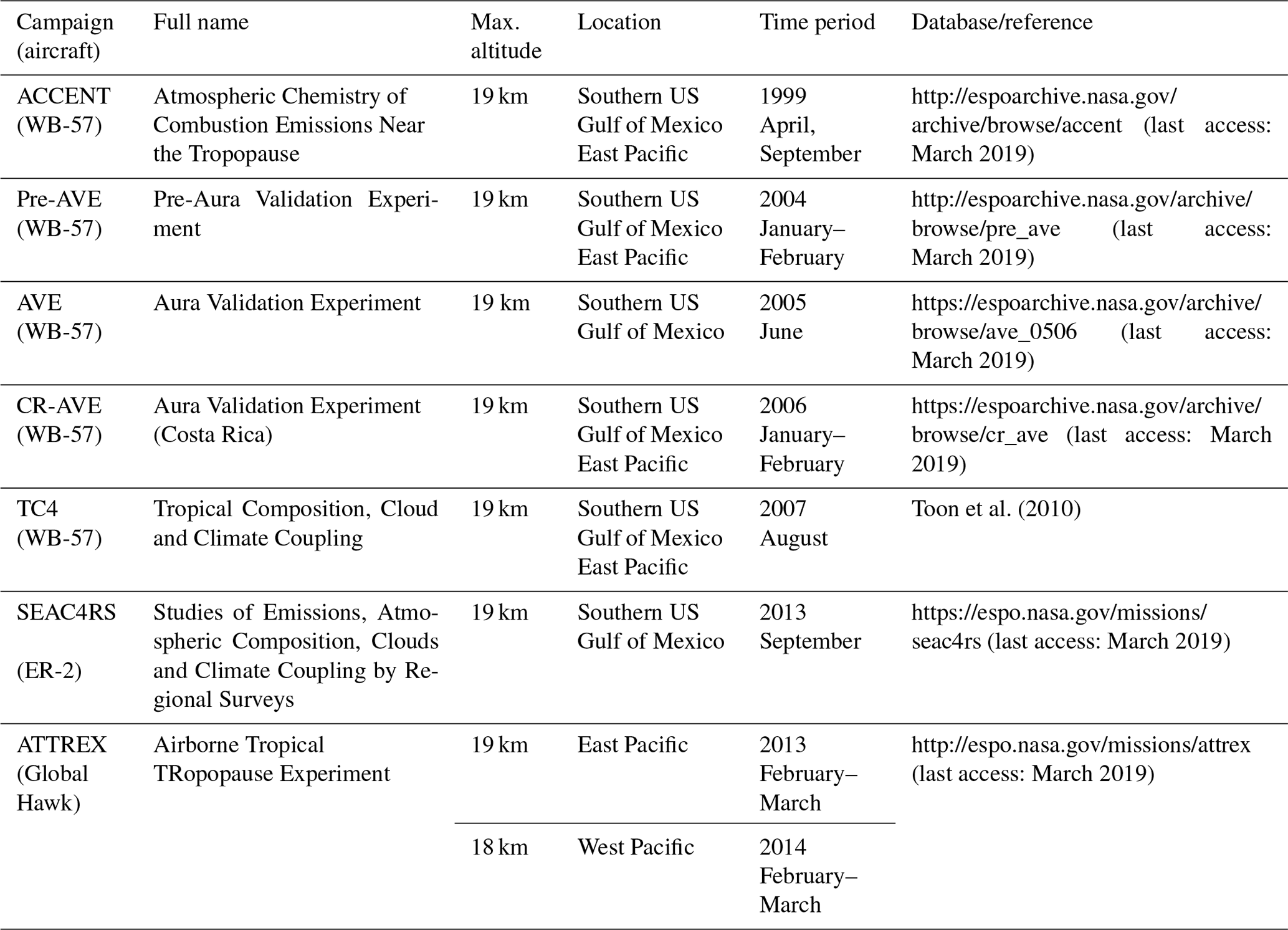
We analyse the spatial and temporal variability of CHBr₃ in the TTL based on the comparison of Lagrangian transport simulations to data from aircraft campaigns. CHBr₃ measurements in the upper TTL are currently available from seven aircraft campaigns. Nearly all of the campaigns took place over Central America, except for the Airborne Tropical TRopopause EXperiment (ATTREX) campaign which was in large part conducted over the Pacific. Detailed information about the aircraft missions including location and time period is presented in Table 1.

Table 1Aircraft campaigns with CHBr₃ measurements used in the study.

Download Print Version | Download XLSX

2.3 VSLS transport modelling

We are interested in the direct contribution of CHBr₃ and CH₂Br₂ to the stratospheric halogen loading in the form of source and product gas contributions. Therefore, the atmospheric transport of the two compounds from the oceanic surface into the upper troposphere and TTL is simulated with the FLEXPART Lagrangian particle dispersion model (Version 9.2 beta; Stohl et al., 2005, 2010). The oceanic emissions, based on the air–sea flux data from Ziska et al. (2013), prescribe the amount of CHBr₃ and CH₂Br₂ released in the FLEXPART simulations with each air parcel trajectory. The global air–sea flux, given on a 1^∘ × 1^∘ grid, is used here at a monthly mean temporal resolution. For CHBr₃, 90 trajectories are released per month from each grid box carrying the gas amount prescribed by the emission scenario. For the longer-lived CH₂Br₂, 45 trajectories are released per month. Once all brominated SGs and PGs have been removed from a trajectory through chemical decay and wet deposition, the trajectory is automatically terminated, so that the number of all active trajectories stays roughly constant (∼20 million) at all times after the initial spin-up period. The global CHBr₃ simulations are run for 35 years from 1979 to 2013 with a spin-up period of 6 months in order to analyse in detail the spatial–temporal variability and long-term changes of stratospheric injection. For the longer-lived CH₂Br₂, the spatial–temporal variability is known to be much smaller (Hossaini et al., 2010), and runs are carried out for 3 years from 2011 to 2013 with a spin-up period of 18 months.

The transport in FLEXPART is driven by meteorological fields from the ECMWF (European Centre for Medium-Range Weather Forecasts) reanalysis model. FLEXPART includes parameterizations for moist convection (Forster et al., 2007) and turbulence in the boundary layer and free troposphere (Stohl and Thomson, 1999), dry deposition, and scavenging (Stohl et al., 2005). The runs are based on the 6-hourly fields of horizontal and vertical wind, temperature, specific humidity, convective precipitation, and large-scale precipitation from the ECMWF reanalysis product ERA-Interim (Dee et al., 2011) given at a horizontal resolution of 1^∘ × 1^∘ on 60 model levels. A preprocessor retrieves the meteorological fields from the ECMWF archive, including the vertical wind, which is calculated in hybrid coordinates mass-consistently from spectral data. FLEXPART has been validated based on comparisons with measurement data from three large-scale tracer experiments (Stohl et al., 1998) and with results from intercontinental air pollution transport studies (e.g. Forster et al., 2001; Stohl and Trickl, 1999). Previous FLEXPART studies using a similar model setup as applied here have shown a very good agreement between diagnosed and observed VSLS profiles (e.g. Tegtmeier et al., 2013; Fuhlbrügge et al., 2016).

FLEXPART includes the simulation of chemical decay by reducing the tracer mass carried by each air parcel corresponding to its prescribed chemical lifetime. We set the atmospheric lifetime of CHBr₃ (CH₂Br₂) to an altitude-dependent lifetime profile ranging from 16 (50) d at the ocean surface to 29 (400) d in the TTL (Hossaini et al., 2012b). The lifetime profiles were derived from simulations of the chemical tropospheric loss processes of CHBr₃ and CH₂Br₂ with the chemical transport model TOMCAT (Chipperfield, 2006). Previously, profiles from TOMCAT have been shown to agree well with aircraft observations in the tropical troposphere (Hossaini et al., 2012b).

The bromine resulting from the photochemical loss of CHBr₃ and CH₂Br₂, based on prescribed loss terms, contributes to the inorganic product gases. In the FLEXPART simulations, these product gases are grouped together as Br_y and transported together with the VSLS source gases along the trajectory. Thus, we assume instantaneous conversion between organic intermediate product gases and Br_y, which has been shown to be reasonable by Hossaini et al. (2010). Br_y can be removed effectively from the troposphere through wet scavenging by rain or ice (Yang et al., 2005). FLEXPART includes in-cloud as well as below-cloud scavenging, which is initiated if the relative humidity as calculated from meteorological input data exceeds 80 % and the precipitation rate is larger than zero. In FLEXPART, the cloud scavenging ratio is used to model washout of soluble species. The ratio is calculated within FLEXPART with the help of the effective Henry's law coefficient, H_eff, which describes the physical solubility of a species as well as the effects of dissociation. Among the members of the Br_y family, HBr and HOBr can be washed out while the remaining species Br, BrO, BrONO₂, and Br₂ are not soluble. HBr has a very large acidity dissociation constant resulting in an effective Henry's law coefficient of 7.1×10¹³ M atm⁻¹ for T=298 K and pH = 5 (Yang et al., 2005). While HBr provides the main pathway for wet removal of inorganic Br_y, HOBr is also soluble due to physical solubility, but not due to dissociation (Frenzel et al., 1998) with $H_{\mathrm{eff}}=\mathrm{6.1}\times {\mathrm{10}}^{\mathrm{3}}$ M atm⁻¹. In order to determine which fractions of Br_y are in the form of HBr and HOBr, we apply the Br_y partitioning derived from p-TOMCAT simulations (Yang et al., 2010).

Based on analysed wind fields together with complex chemical schemes, p-TOMCAT simulates the tracer distribution in the troposphere and lower stratosphere including gaseous phase bromine chemistry. The three-dimensional Br_y field from p-TOMCAT and its partitioning into HOBr, HBr, Br, BrO, BrONO₂, and Br₂ are given at a time step of 30 min. As the partitioning of the Br_y field varies strongly with location and time, we apply it in a first step to every air parcel according to its location each time before the wet deposition is initiated. In a second step, wet deposition is calculated individually for each inorganic bromine species based on its solubility specified by the effective Henry's law coefficient, as described above. Once wet deposition is initiated the Br_y fraction determined to be washed out is removed completely.

Dissolved inorganic bromine can be released back to the gas phase by heterogeneous chemical reactions (Abbatt, 2003; Salawitch, 2006), extending the tropospheric lifetime of Br_y by altering the efficiency of wet deposition (von Glasow et al., 2004). The heterogeneous reactions on aerosols which reactivate bromine radicals from the reservoir species (Yang et al., 2005, 2010) are included in the chemical scheme of p-TOMCAT. This release of bromine back to the gas phase results in elevated BrO∕Br_y ratios (Yang et al., 2010), and thus a lower fraction of Br_y is subject to wet deposition compared to a scenario without the heterogeneous chemical reactions. As we use the p-TOMCAT Br_y partitioning for our trajectory simulations, these aerosol effects have indirectly been taken into account when simulating the wet removal of Br_y. Uncertainties in the modelled wet deposition arise from the parameterization of solubility via the effective Henry's law coefficient and from uncertainties in the Br_y partitioning caused by errors in the aerosol loading and in the mechanism used for heterogeneous reactions. Clouds and aerosols within p-TOMCAT are not matched with those in FLEXPART, which might lead to an additional error source.

For the analysis of the spatial and temporal variability of CHBr₃ in the TTL from FLEXPART simulations and aircraft observations in Sect. 3.1 to 3.5, we use mixing ratios at 17 km (approximate cold point) and mixing ratios averaged over 16–18 km (upper part of the TTL). In order to derive the amount of VSLS source and product gases entrained into the stratosphere from the model simulations in Sect. 3.6, we explicitly calculate the cold point along each trajectory based on the ERA-Interim meteorological fields as stratospheric entrainment point. The derived estimates of stratospheric VSLS entrainment depend on the meteorological input data sets and on various FLEXPART model parameters, such as the convective parameterization. The accurate representation of convection has been validated with tracer experiments and ²²²Rn measurements (Forster et al., 2007). The application of transport timescales based on vertical heating rates instead of vertical wind fields in the TTL between 15 and 17 km results in only minor differences of VSLS entrainment (Tegtmeier et al., 2012).

3.1 CHBr₃ in the TTL

Figure 1a shows the long-term annual mean CHBr₃ distribution at 17 km as derived from the Lagrangian transport calculations driven by monthly mean oceanic emission fields for the time period 1979–2013. Clearly, CHBr₃ has a very pronounced spatial variability due to its short lifetime. The largest CHBr₃ mixing ratios of up to 0.4 to 0.5 ppt can be found over (1) Central America, (2) the Maritime Continent and the tropical west Pacific, and (3) the tropical Indian Ocean (all regions are highlighted by black squares in Fig. 1a labelled from 1 to 3). Other tropical regions with only little convective uplift show smaller mixing ratios, mostly between 0.1 and 0.2 ppt.

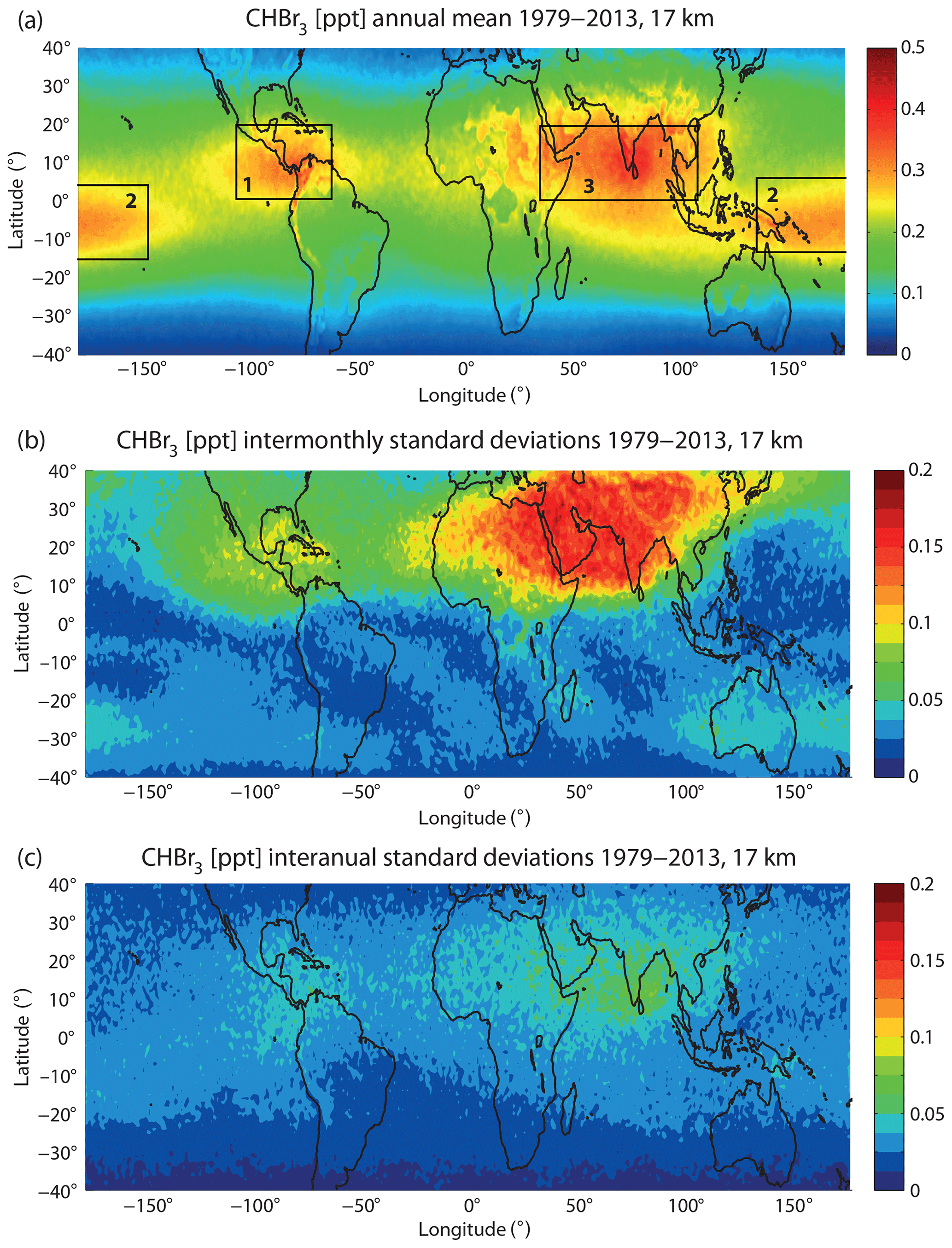
Figure 1Modelled annual mean distribution of CHBr₃ at 17 km for 1979–2013 (a) and the inter-monthly (b) and inter-annual (c) variations given by the standard deviations over all monthly, multi-annual mean, and annual mean values, respectively. Rectangles stand for regions of maximum CHBr₃ mixing ratios and will be discussed in detail in Sect. 3.2 to 3.4.

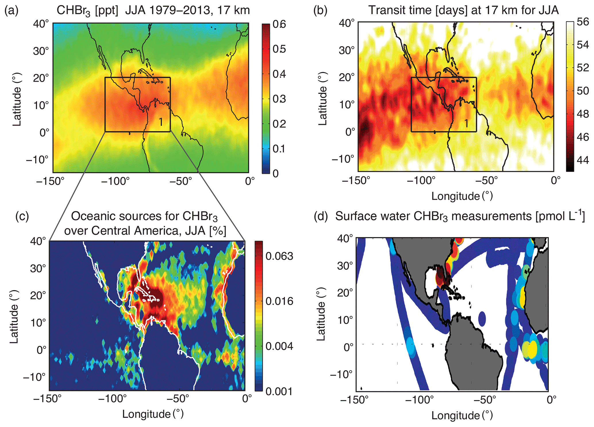
Figure 2Modelled distribution of CHBr₃ at 17 km for JJA, 1979–2013 (a), transit time of air masses from the ocean surface to the TTL (b), oceanic source regions for CHBr₃ (c), and measurements of oceanic CHBr₃ concentrations from the HalOcAt database used for Ziska et al. (2013) (d). The oceanic source regions in (c) are colour coded according to their contribution (% per 1^∘ × 1^∘ grid box) to the amount of CHBr₃ at 17 km in the black box over Central America (highlighted in a and b).

Entrainment of CHBr₃ into the stratosphere also shows a large temporal variability. The seasonal variability is given here by the standard deviation over all monthly, multi-annual mean values (Fig. 1b). The by far most pronounced variability is found in the region of the Asian monsoon anticyclone, which is characterized by a strong seasonality of vertical transport processes (Randel et al., 2010). Furthermore, the distribution of CHBr₃ at the cold point over Central America shows some seasonal variations, however, of smaller magnitude. The Maritime Continent and tropical west Pacific have only a very weak seasonal cycle. Overall, the seasonal variations are more pronounced in the Northern Hemisphere (NH) tropics and quite low in the Southern Hemisphere (SH) tropics. Seasonal CHBr₃ entrainment averaged over 1979–2013 is shown in the Supplement (Fig. S2).

Inter-annual variations are given in the form of the standard deviation over all annual mean CHBr₃ mixing ratios at 17 km (Fig. 1c). In comparison to the seasonal variability, the inter-annual variability is relatively small in the NH tropics but is of similar magnitude in the SH tropics. Drivers of the seasonal and inter-annual variability will be discussed in the following sections. We will analyse the three regions with maximum CHBr₃ entrainment identified above and investigate the relative importance of emissions and transport processes for the overall distribution and seasonality of stratospheric injection.

3.2 Central America

CHBr₃ in the TTL, on its way from the ocean surface to the stratosphere, shows a pronounced maximum over Central America between 0–20^∘ N and 60–110^∘ W (black square in Figs. 1a and 2a). This maximum is present all year, but most pronounced during NH summer and autumn. In the following, we will use the simulations for June–July–August to address the question of whether this maximum arises from very strong oceanic sources or from strong convective transport. The impact of transport on the CHBr₃ distribution in the upper TTL is analysed by estimating the time air masses need from the ocean surface to 17 km based on the FLEXPART model simulations. The transport time of each trajectory is assigned to the location where the trajectory reaches 17 km. A map of the “ocean surface–17 km transit times” is derived by averaging over all trajectories on a 1^∘ × 1^∘ grid. The tropical annual mean transit time is around 55 d with variations between 45 and 70 d (not shown here). Transit times over Central America for the June–July–August season are relatively short with values around 48 d (Fig. 2b). However, the transit times over the east and central Pacific are similar or even shorter, suggesting that the vertical transport in this region is as efficient as over Central America. Therefore, atmospheric transport timescales alone cannot explain the CHBr₃ maximum over Central America.

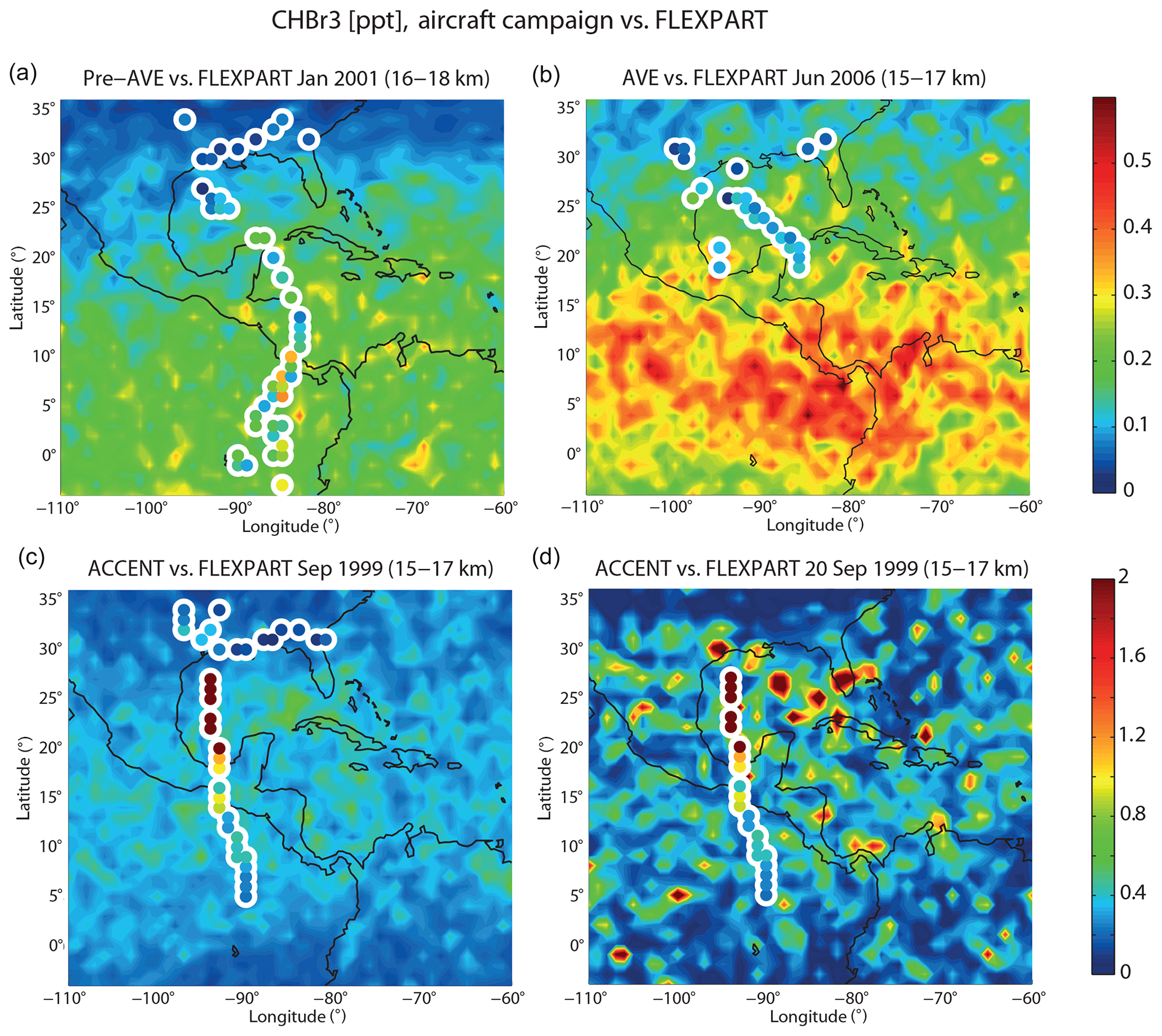
Figure 3Modelled distribution of CHBr₃ in the upper TTL from FLEXPART (background colouring) in comparison with aircraft campaign measurements (coloured symbols with white edges). In (a), (b), and (c), all individual measurements from the respective campaign and the model mean over the same time period are shown. Only in (d) is one individual flight (ACCENT flight from 20 September 1999) shown together with FLEXPART daily mean values to illustrate the large spatial variability including maximum values ≥2 ppt.

In addition to the transit time, we analyse the oceanic sources of CHBr₃ over Central America. Each trajectory reaching the TTL over Central America (black square in Fig. 2a) contributes a certain amount of CHBr₃ to this local maximum by carrying its prescribed oceanic emission (Ziska et al., 2013) from the surface to the cold point. The relative contribution (%) of each trajectory is assigned to its oceanic release point, thus quantifying which ocean region contributes the largest amounts of CHBr₃ to the local maximum in the TTL. The relative contributions averaged over 1^∘ × 1^∘ grid cells (Fig. 2c) demonstrate that the largest sources stem from the Gulf of Mexico, the Caribbean Sea, and the western North Atlantic. Some smaller contributions come from the west coast of North Africa and from the equatorial Atlantic. The co-occurrence of strong sources and the relatively short transport timescales over the Caribbean Sea and Central America mainly cause the local CHBr₃ maximum in the Central American TTL. While transport timescales are also short (or even shorter) in the eastern Pacific, oceanic emissions are very small there, and vice versa more pronounced emissions over the Atlantic and along the coast of Africa do not cause a global maximum due to longer transport timescales.

The regional oceanic measurements in surface water, which were used to derive the extrapolated concentration and emission maps (Ziska et al., 2013), are given in Fig. 2d. The available data show, in particular, high oceanic CHBr₃ concentrations at the Florida coastline and in the eastern part of the Gulf of Mexico. A reasonable number of measurements with a distinctive distribution are available in this region, supporting the extrapolated climatological source distribution, which leads to the CHBr₃ maximum in the TTL over Central America discussed above.

Over the last decades, the atmospheric distribution of CHBr₃ over Central America has been investigated by a number of different aircraft campaigns. We will use available upper air measurements to evaluate the distribution and variability of the model-derived CHBr₃ fields. Details of the aircraft campaigns are given in Table 1. We show the spatial CHBr₃ distribution in the TTL as observed during three different campaigns in comparison to the model simulations (Fig. 3). The altitude ranges in the upper TTL have been chosen so that each comparison includes a maximum number of observational data. While for the aircraft campaigns individual measurements are shown at the measurement locations, the model fields are averaged over the duration of the respective campaign. This method allows us to evaluate the spatial distribution of measured and modelled CHBr₃ fields, but it has the disadvantage of comparing in situ data with temporally averaged fields. We will discuss how this can impact the comparison and how the temporal variability can be taken into account.

For the Pre-AVE campaign during NH winter, CHBr₃ in the upper TTL (16–18 km) shows a latitudinal gradient with small values of 0–0.1 ppt in the northern subtropics and with higher values of up to 0.3–0.4 ppt around the Equator. The same gradient is also evident from the model simulation, resulting in an overall good agreement. Similarly, for the AVE campaign during NH summer, both the observations and the model results show a latitudinal gradient with increasing values towards lower latitudes. However, here the overall agreement is poor, since the model results are on average 50 % larger than the measurements.

Finally, for the ACCENT campaign during NH autumn, the observations reveal extremely high CHBr₃ (up to 2 ppt) between 30 and 20^∘ N. While CHBr₃ is decreasing north and south of this area towards the range of 0.5–1 ppt, the values are still very high when compared to other campaigns over Central America. FLEXPART results, averaged over the time period of the ACCENT campaign (September 1999), show the largest monthly mean CHBr₃ values of around 0.7 ppt, which are substantially smaller than the observations of 2 ppt. However, the model results look quite different and show large spatial inhomogeneities when evaluated at a daily mean resolution. Maximum model values are much higher for the daily resolution and in some locations, very close to the flight track, of similar size as the observations (around 2 ppt). The spotty features in the model simulations are a result of the high oceanic sources directly underneath interacting with localized convective transport. The latter brings localized air masses with very high CHBr₃ mixing ratios from the boundary layer into the 15–17 km layer. The differences between monthly and daily mean model values make clear that CHBr₃ model–measurement comparisons may be obscured by the high variability of the field. Given this high variability and the existing uncertainties in the diagnosed oceanic sources and atmospheric transport processes, it is very difficult for a model to predict the correct in situ values at a given time and measurement position. Nevertheless, if the large-scale emissions and transport fields are correct, spatial and temporal averaging of the model results can be expected to produce realistic mean VSLS fields and to improve the agreement with observations. Only in cases where rare events have been observed will averaging the CHBr₃ fields not necessarily lead to a better agreement with the measurements, as demonstrated above for the ACCENT campaign. Consequently, it is important to include estimates of the spatial and temporal variability of the CHBr₃ field in all comparisons.

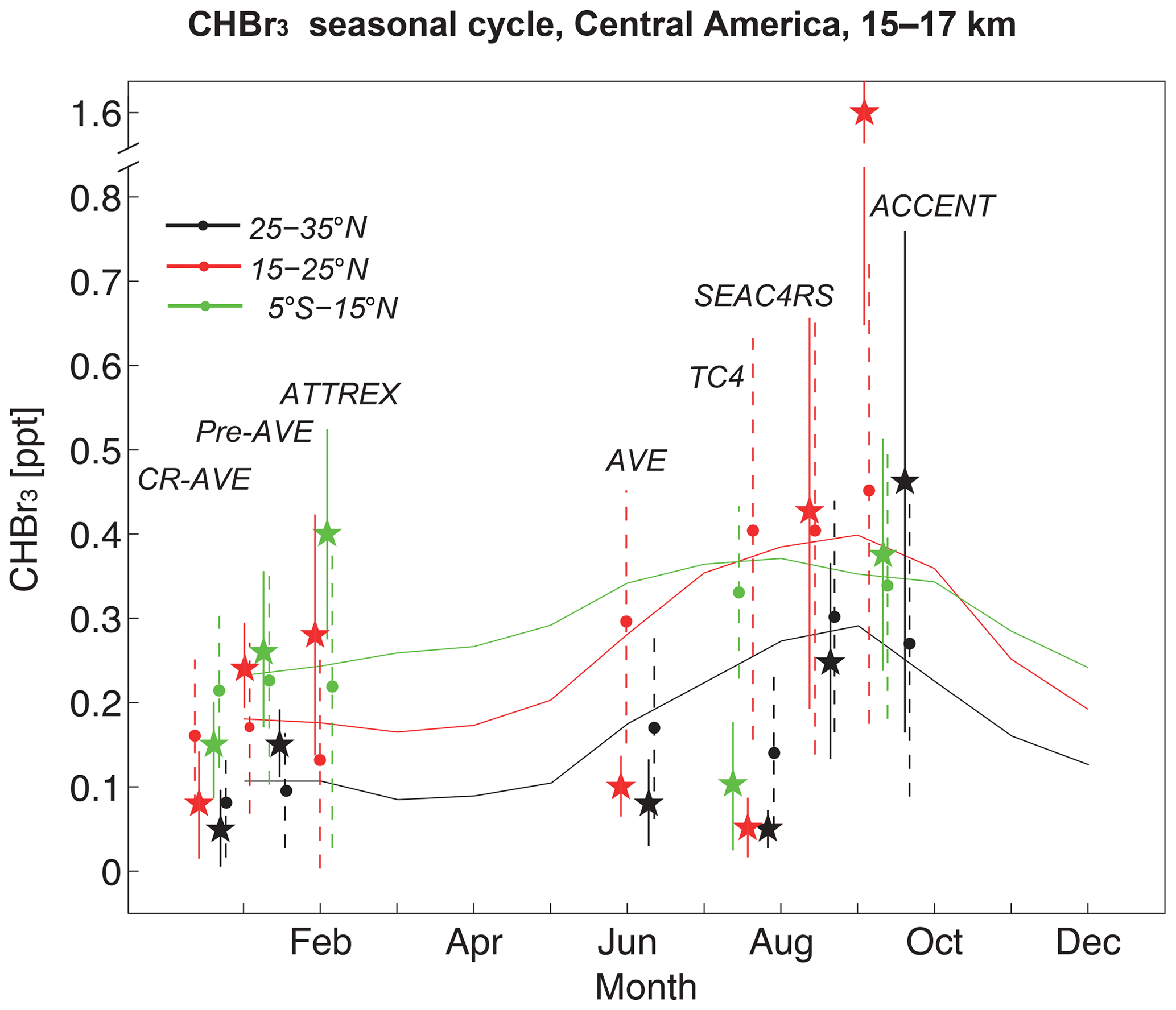
Figure 4Seasonal cycle of CHBr₃ in the upper TTL (15–17 km) over Central America from FLEXPART simulations (solid lines) averaged over 110–80^∘ W and 5^∘ S–15^∘ N (green), 15–25^∘ N (red), and 25–35^∘ N (black) for 1999–2013. In addition, aircraft measurements (stars) and coincident FLEXPART values (filled circles) are shown averaged over the same latitude bins and corresponding to the respective year of the campaign. Temporal and spatial variability of average measurements (solid vertical lines) and coincident model values (dashed vertical lines) is shown in the form of the 1-sigma standard deviation over all values in the respective bin.

Download

A summary of the CHBr₃ model results compared to aircraft campaigns in the Central American region, taking into account spatial and temporal variability, is provided in Fig. 4. Here, we compare measurements averaged over different parts of the flight tracks (split by latitude) with FLEXPART coincidences averaged over the same latitudinal bins. The variability of the CHBr₃ distribution from observations and coincident model values is given by the standard deviation over all values in the respective region. In addition, the FLEXPART seasonal cycle averaged over 110–80^∘ W, the main longitudinal extent of the aircraft campaigns, and the entire campaign time period (1999–2013), is shown. The comparison of the three campaigns during NH winter shows an overall good agreement. For some latitude bins, the modelled mean values agree very well with the observations (e.g. Pre-AVE for 5^∘ S–15^∘ N); for other regions, differences of the mean values can be up to 50 %–100 %. However, all observational mean values are within the standard deviations of the modelled field, indicating good agreement of model and measurements.

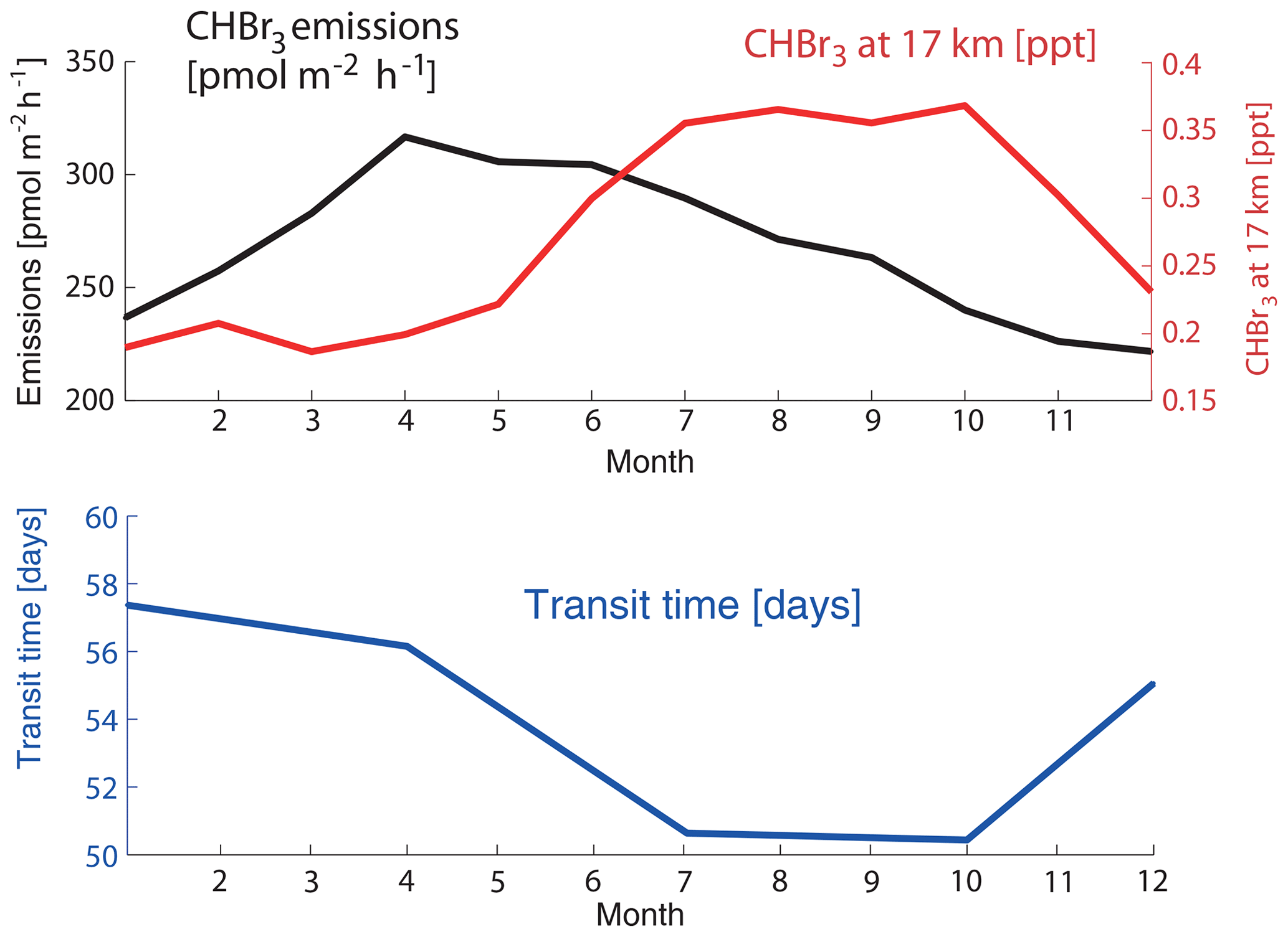
Figure 5Seasonal cycles of CHBr₃ at 17 km over Central America (black square in Fig. 2a) from FLEXPART simulations (red line), oceanic CHBr₃ emissions averaged over the respective source region (black line), and the “surface–17 km” mean transit time (blue line) are shown.

Download

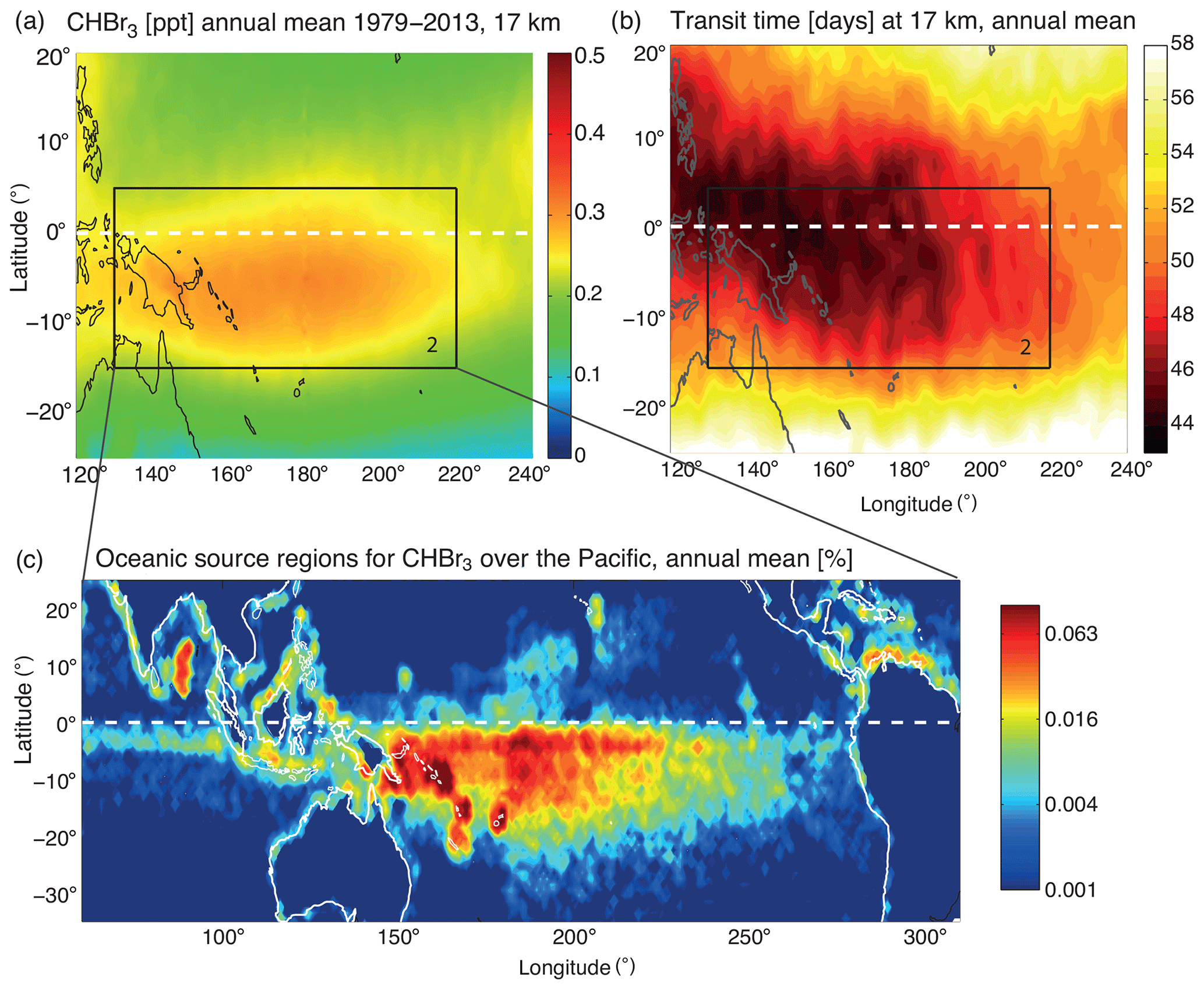
Figure 6Modelled distribution of CHBr₃ at 17 km, annual mean 1979–2013 (a), transit time of air masses from the ocean surface to the TTL (b), and oceanic source regions for CHBr₃ at 17 km (c). Oceanic source regions are colour coded according to their contribution (% per 1^∘ × 1^∘ grid box) to the amount of CHBr₃ at 17 km in the black box over the west Pacific (highlighted in a and b).

For the campaigns during NH summer, mean differences are in general larger than during NH winter. At the same time, the temporal and spatial variability of the simulated and observed CHBr₃ distribution is also larger so that most observations agree with the coincident model values within their uncertainties. The large differences between the individual campaigns during NH summer confirm the increased variability suggested by the model results. For two of the campaigns (AVE and TC4), FLEXPART overestimates the CHBr₃ values during this time of the year, while for the other two campaigns (SEAC4RS and ACCENT), the observations and modelled values agree relatively well except for one outlier. Particularly high CHBr₃ exists for the 15–25^∘ N region, observed during the ACCENT campaign at the top altitude of a plume extending from 14 to 16 km near Houston, Texas. This value is larger than the model mean, although observational and model value uncertainties slightly overlap. In total, observations and model agree reasonably well with a larger variability during the NH summer and early autumn period. For this time of the year, the model also suggests a seasonal CHBr₃ maximum which is confirmed by measurements from SEAC4RS and ACCENT, but not by the AVE and TC4 campaigns.

CHBr₃ in the upper TTL over Central America shows pronounced seasonal variations as revealed by the comparisons to aircraft campaigns in Fig. 4. The CHBr₃ seasonal cycle at 17 km shows a maximum from July to October (∼0.37 ppt) and a minimum from January to April (∼0.17 ppt) (Fig. 5a). Such seasonal variations can be caused by variations in the oceanic emissions or the atmospheric transport times. First, we analyse the seasonal cycle of CHBr₃ emissions, averaged over the source region identified earlier, which show peak emissions from April to June of up to 320 pmol m⁻² h⁻¹. This peak in surface emissions in late spring–early summer is consistent with a peak in the TTL around 2 months later, as the mean transit time from the surface to 17 km in this region is about 55 d. Second, we analyse the seasonal cycle of the transit time and find a minimum from July to October, which is also consistent with the highest CHBr₃ values in the TTL during the same time period. While the amplitude of the seasonal cycle in CHBr₃ in the TTL is around 74 %, seasonal variation in the emissions and the transit time are only 36 % and 15 %, respectively. However, the amplitude in transit time does not directly translate into the amplitude in CHBr₃ in the TTL, given the logarithmic nature of the atmospheric lifetime of chemical compounds. Overall, the interaction of both processes, oceanic emissions and atmospheric transport, causes the pronounced seasonal cycle of CHBr₃ over Central America.

3.3 Maritime Continent and tropical west Pacific

CHBr₃ in the TTL shows a pronounced maximum over the Maritime Continent and tropical west Pacific between 15^∘ S–5^∘ N and 130–220^∘ E (black square in Figs. 1a and 6a). An important characteristic of this CHBr₃ maximum (referred to as the west Pacific maximum hereinafter) is that the high values are not distributed symmetrically across the Equator but are shifted southwards. The maximum is present all year with no pronounced seasonal cycle (see Fig. 1b). In the following, we will use annual mean results to investigate if the high values arise from very strong oceanic sources or from strong convective transport. The transit time shows the smallest values of around 45 d in the west Pacific and over the Maritime Continent (Fig. 6b). The most important deviation from the CHBr₃ distribution at 17 km is that over the west Pacific the shortest timescales and thus most efficient transport are not centred in the SH, but they are distributed symmetrically across the Equator.

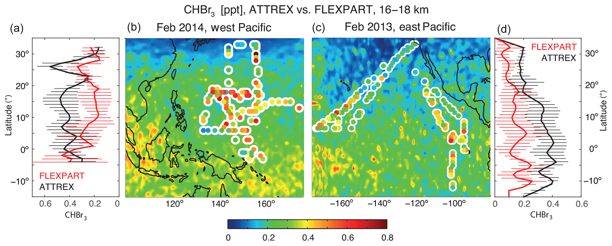
Figure 7Modelled distribution of CHBr₃ in the uppermost TTL from FLEXPART (background colouring) in comparison with ATTREX aircraft campaign measurements (coloured symbols with white edges) is given in (b) and (c). Zonal means of coincident model–measurement comparisons are given in (a) for FLEXPART and the ATTREX campaign in February–March 2014 in the west Pacific and in (d) for FLEXPART and the ATTREX campaign in February–March 2013 in the east Pacific. Temporal and spatial variability of measurements and coincident model values is shown in form of the 1σ standard deviations over all values in the respective zonal bin (horizontal lines).

Oceanic sources for CHBr₃ in the west Pacific upper TTL (black square in Fig. 6a) stem mostly from the Pacific Ocean, the Maritime Continent, and also to a smaller degree Central America (Fig. 6c). The trajectory analysis clearly shows that the largest contribution comes from the west Pacific south of the Equator, while the oceanic contributions north of the Equator are lower. This pattern is directly related to the emission inventory used in this study (Ziska et al., 2013), which suggests overall stronger emissions in the southern Pacific Ocean (see Fig. S1 in the Supplement). However, available open-ocean surface measurements in both the NH and SH Pacific Ocean were sparse during the time of the construction of the inventory and mostly based on the TransBrom Sonne campaign (Krüger and Quack, 2013). The latitudinal gradient of the emission inventory with stronger emissions in the SH is based on the in situ measurements along one cruise track from Japan to Australia during October 2009 and may not be representative for other seasons and other west Pacific regions. Future ship campaigns are necessary to confirm or improve the existing emission inventory.

Pacific aircraft campaigns are used to further analyse the hemispheric differences of the diagnosed CHBr₃ distribution. ATTREX measurements in the west Pacific in 2014 and in the east Pacific in 2013 are compared to FLEXPART simulations in Fig. 7. In both regions, the comparison reveals a reasonably good agreement with increasing CHBr₃ values towards lower latitudes. In the west Pacific, measurements and coincident model values agree best south of 10^∘ N, while north of this the model underestimates observations by up to 0.3 ppt. In the east Pacific, model values and measurements are closer in the NH and agree mostly within their error bars. South of the Equator, however, measurements are constantly larger with differences of up to 0.3 ppt. In total, the modelled CHBr₃ entrainment over the Pacific is too small when compared to measurements, which could be due to an underestimation of the oceanic emissions in this region.

3.4 Tropical Indian Ocean

Annual mean CHBr₃ in the uppermost TTL shows a pronounced maximum over India, the Bay of Bengal, and the Arabian Sea between 2–22^∘ N and 35–110^∘ E (Fig. 1a, referred to as the Indian Ocean maximum hereinafter). The simulations diagnose the globally highest TTL CHBr₃ values of up to 0.5 ppt in the long-term mean over the southern tip of India. At the same time, the intermonthly standard deviation is very high over this region (Fig. 1b) due to pronounced seasonal variations. During NH summer (June–July–August), high CHBr₃ values of around 0.6 ppt are found over a large region stretching from South East Asia all the way to northeast Africa between 10 and 25^∘ N. During SH summer (December–January–February), smaller maximum values of around 0.4 ppt CHBr₃ are diagnosed south of India over the Indian Ocean between 5^∘ S and 10^∘ N (Fig. 8).

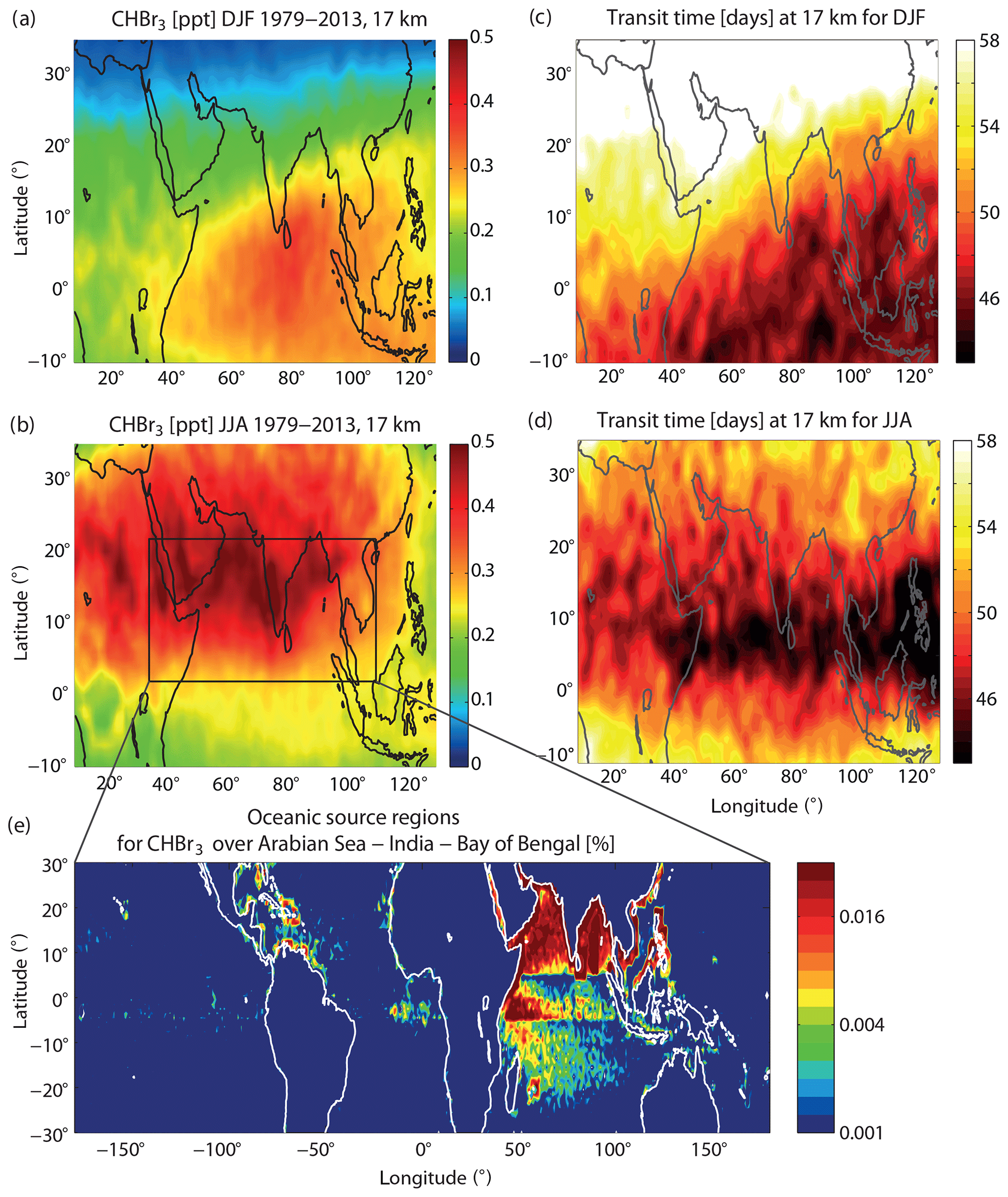
Figure 8Modelled distribution of CHBr₃ at 17 km for DJF and JJA 1979–2013 (a, b). Transit time of air masses from the ocean surface to the TTL for DJF and JJA (c, d). Oceanic source regions colour coded according to their contribution to CHBr₃ at 17 km over Arabian Sea, India, and Bay of Bengal (black box in b) given in percent per 1^∘ × 1^∘ grid box (e).

In order to evaluate the transport efficiency for oceanic short-lived trace gases in this region, the transit time is calculated from the trajectory analysis for the NH and SH summer seasons. During NH winter, transit times from the surface to the TTL show a very similar pattern as CHBr₃ in the TTL, with the shortest transit times of around 45 d over the Indian Ocean coinciding with the largest CHBr₃ abundance. During NH summer, on the other hand, the transit times minimize not in the region of maximum CHBr₃ abundance, but instead south of this region where air masses can reach the TTL within 43 d. Between 10 and 25^∘ N, the transport is still fast and the transit of short-lived species from their ocean sources will take around 48 d. Overall the transit time is similar to values found for the west Pacific and cannot solely account for the simulated maximum CHBr₃ values.

CHBr₃ contributing to the Indian Ocean TTL maximum mostly stems from the Bay of Bengal, the Arabian Sea, the equatorial region of the Indian Ocean, and the coastlines of South East Asian countries like China. Compared to the oceanic contributions identified for the Central America and west Pacific maxima, sources for the Indian Ocean CHBr₃ maxima show a large regional extent including coastal and open-ocean emissions from 20^∘ S to 30^∘ N. Given that oceanic emissions from large parts of the Indian Ocean and adjacent coastal areas can be transported into the Asian monsoon region (Fiehn et al., 2017), the CHBr₃ maxima can be explained by the strong oceanic emissions in this region combined with efficient boundary layer–TTL transport.

The global maximum of CHBr₃ over India, Bay of Bengal, and the Arabian Sea is also subject to the largest uncertainties when compared to the other maxima found in our model simulations. For the construction of the emission inventory from Ziska et al. (2013), only one data set was available for the Indian Ocean (Yamamoto et al., 2001). The data set is based on measurements at seven stations in the open-ocean waters of the Bay of Bengal and reveals relatively high CHBr₃ values between 8 and 15 ng L⁻¹. Given the great distance of the sampling points from the coasts, the authors hypothesized that planktonic production is the most probable source for this high CHBr₃ abundance. Independent measurements from the OASIS campaign in 2014 confirm the subtropical and tropical west Indian Ocean as a strong source for CHBr₃ to the atmosphere, although open-ocean surface concentrations were overall lower with maximum values of 8 ng L⁻¹ (Fiehn et al., 2017). A recent update of the Ziska bottom-up CHBr₃ emission climatology (Fiehn et al., 2018b) suggests enhanced emissions in the tropical Indian Ocean, which would lead to even higher stratospheric entrainment in this region. While the high values from Yamamoto et al. (2001) were used locally for the emission climatology, the rest of the tropical Indian Ocean was filled by applying open-ocean data from the tropical Atlantic and Pacific. Consequently, the emission scenario for the Indian Ocean has large uncertainties, and further VSLS measurements are required to confirm or improve our estimates of the Indian Ocean as the region of strongest CHBr₃ entrainment into the stratosphere.

3.5 Inter-annual and long-term changes

Long-term changes of tropical mean (30^∘ N–30^∘ S) CHBr₃ mixing ratios at 17 km show a weak but significant trend of 0.017±0.012 ppt Br per decade, corresponding to a 10 % increase in CHBr₃ over the whole time period (1979–2013). Regionally, the long-term changes are more pronounced and FLEXPART simulations suggest decreasing or increasing CHBr₃ in the TTL depending on the location (Fig. 9). Over South America, Australia, and the central–east Pacific, the trend is not significant given the relatively small trend values compared to the inter-annual variability found here. For all other regions, CHBr₃ shows a significant positive trend of 2 %–10 % per decade. CHBr₃ over the Indian Ocean and Maritime Continent is highlighted in Fig. 9c as the region with the maximum trend (0.04 ppt Br per decade), mostly driven by the steep changes related to El Niño–Southern Oscillation (ENSO) over the time period 2000–2013 (Fiehn et al., 2018a). CHBr₃ over the east Pacific is highlighted in Fig. 9b as an example of a negative but not significant trend (−0.017 ppt Br per decade).

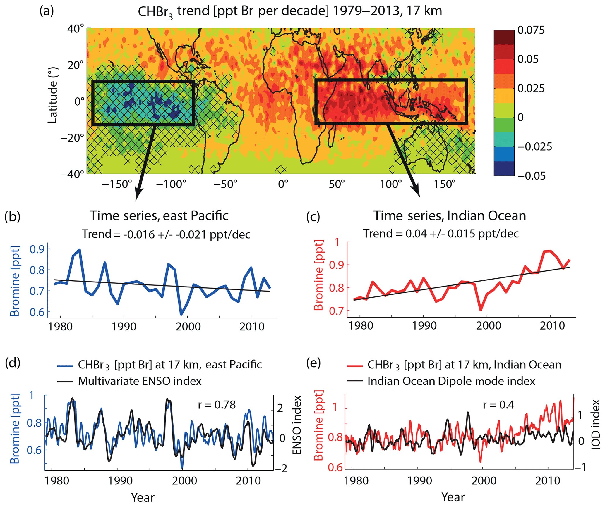
Figure 9Modelled long-term change of CHBr₃ (Br per decade) at 17 km for the time period 1979–2013 (a). Time series (annual means) averaged over the east Pacific and the Indian Ocean–Maritime Continent–west Pacific region are shown together with the trend (b, c). Time series (5-month running mean) are shown together with the ENSO index and Indian Ocean Dipole index (d, e).

The projected inter-annual and long-term changes of CHBr₃ injections are driven by the variability of oceanic emissions (Ziska et al., 2013), convective transport from the surface to the TTL (Aschmann et al., 2011), and transport in the TTL (Krüger et al., 2009). Our model runs are based on CHBr₃ emissions that allow for changes over time due to changing meteorological surface parameters (mostly ERA-Interim) but do not take into account oceanic biogeochemical and related CHBr₃ production changes. Due to increasing sea surface temperature and wind speed, CHBr₃ emissions increase considerably by 7.9 % from 1979 to 2013 (Ziska et al., 2017). Changes in the modelled atmospheric transport are driven by long-term changes in ERA-Interim parameters such as temperature, winds, and humidity fields, leading to an overall trend of CHBr₃ at 17 km of 10 % for 1979–2013.

The two CHBr₃ time series over the east Pacific and Indian Ocean–Maritime Continent (Fig. 9b and c) show the opposite long-term behaviour but also share some of the same patterns of inter-annual variability. In particular, signals like the steep CHBr₃ decrease from 1997/1998 to 1999, the increase from 2008 to 2009/2010, and the relatively high values in 1982 are common to both time series. We analyse the common and separate drivers of the variability of the two time series further by comparing them to modes of tropical climate variability.

First, we compare the time series of stratospheric bromine in the east Pacific with the Multivariate ENSO Index (MEI; Wolter and Timlin, 2011) in Fig. 9d. The irregular ENSO variations in winds and sea surface temperatures over the tropical eastern Pacific Ocean drive changes in CHBr₃ emissions and atmospheric transport, leading to a high correlation of the two time series (r=0.78). During El Niño years, water in the central and eastern Pacific becomes warmer than usual and the dry and steady easterly winds turn into warm and moist westerlies, leading to an increase in the oceanic emissions. This increase is driven by meteorological and oceanic surface variations but does not allow for possible changes in biogenic CHBr₃ production related to changes in the eastern Pacific upwelling system (Hepach et al., 2016). At the same time, the warm east Pacific favours stronger convection, intensifying the VSLS transport into the TTL (Aschmann et al., 2011). Overall, El Niño years lead to enhanced CHBr₃ injection over the east Pacific (e.g. 1982, 1986, 1991, and 1997), while La Niña corresponds to weaker CHBr₃ injection (e.g. 1988, and 2010).

Second, variations in CHBr₃ at 17 km over the Indian Ocean and Maritime Continent are shown together with the Indian Ocean Dipole (IOD) mode index (Fig. 9e), an indicator of the east–west temperature gradient across the tropical Indian Ocean (Saji et al., 1999). The two time series are weakly correlated (r=0.4), sharing some of their variability. The IOD is a coupled ocean–atmosphere phenomenon with anomalous cooling of the southeastern tropical Indian Ocean and anomalous warming of the western tropical Indian Ocean during a positive phase. Associated with these changes the convection normally situated over the eastern Indian Ocean warm pool shifts to the west. For some years, the positive phase results in slightly stronger CHBr₃ emissions and more effective atmospheric transport (e.g. 1982–1983, 2006). In other years, strong IOD events will not impact the CHBr₃ abundance over the Indian Ocean–Maritime Continent (e.g. 1997–1998). The relatively weak correlation of CHBr₃ injection and IOD results from the influence of the ENSO signal on atmospheric transport in this region. A combination of sea surface temperature (SST) anomalies in the west Indian Ocean and the ENSO signal can have varying impacts on the CHBr₃ injection depending on the time of year (Fiehn et al., 2018a). While positive SST anomalies together with El Niño conditions in boreal winter and spring enhance stratospheric VSLS injection, La Niña conditions in boreal autumn can also cause stronger-than-normal stratospheric injection. Overall, the inter-annual variability of the CHBr₃ time series is driven by a combination of the ocean–atmosphere modes in the Indian and Pacific Ocean; however, the strong increase during 2009–2013 is not related to either of the two modes.

The overall pattern of long-term CHBr₃ changes at 17 km shows a strong similarity to the long-term changes in sea surface temperature derived from ERA-Interim data (Fig. 10). While the global mean surface temperature has increased due to anthropogenic greenhouse gas emissions (IPCC, 2007), the spatial pattern of global warming is more complex. Most regions exhibit a warming trend over the 35-year period; however, much of the eastern Pacific cooled. This cooling may either be related to an unusual strong manifestation of internal variability in the observations or be caused by external regional forcings (e.g. Wang et al., 2012; Luo et al., 2012). ERA-Interim long-term temperature changes over the oceans show good agreement with HadCRUT, a combined data set of instrumental temperature records, with only small differences (Simmons et al., 2014). Most interesting for our analysis is the correlation between the SST trends and the long-term changes of stratospheric CHBr₃ entrainment. Regions with large positive SST trends such as the Indian Ocean, east Atlantic, and Maritime Continent coincide with regions where the CHBr₃ entrainment trend is strongest. The east Pacific, on the other hand, stands out as the region where the SST cooling trend coincides with decreasing CHBr₃ entrainment. While this relation holds for many oceanic regions, we also find outliers such as the southern Indian Ocean, where SST trends are around zero but CHBr₃ entrainment shows a strong positive trend. Based on our modelling approach, the interaction of two mechanisms causes the strong correlation between the SST and CHBr₃ trends. Higher sea surface temperatures and stronger surface winds force a larger flux of CHBr₃ out of the ocean into the atmosphere (Ziska et al., 2013) and at the same time cause enhanced convection, transporting surface air masses into the TTL (Tegtmeier et al., 2015). As the cold point tropopause altitude shows no significant trend in radiosondes or ERA-Interim data over the 1980–2013 time period (Tegtmeier et al., 2020), CHBr₃ changes at 17 km correspond directly to changes of stratospheric CHBr₃ entrainment. Future SST changes can be expected to drive a continued positive trend of stratospheric CHBr₃ entrainment (Hossaini et al., 2012a).

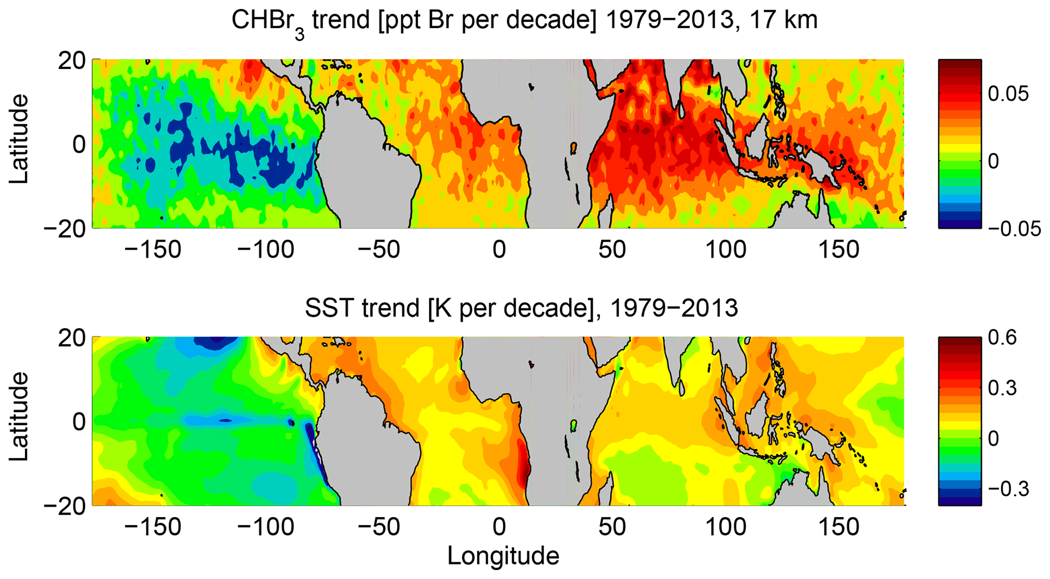
Figure 10Modelled long-term change of FLEXPART CHBr₃ (ppt Br per decade) at 17 km and ERA-Interim sea surface temperature (SST) (K per decade) for the time period 1979–2013.

3.6 Overall CHBr₃ and CH₂Br₂ contribution to stratospheric bromine

CHBr₃ together with CH₂Br₂ provide the main contribution of oceanic bromine to the stratosphere. CH₂Br₂ mixing ratios in the inner tropical belt (10^∘ S–10^∘ N) show less variability than CHBr₃, consistent with the longer lifetime, and range between 0.9 and 1.4 ppt. The largest values can be detected over the west and central Pacific and are distributed evenly over both hemispheres (Fig. 11). There is no local CH₂Br₂ maxima over the Indian Ocean, as observed for CHBr₃, since no strong localized sources in the region exist according to the Ziska et al. (2013) climatology. However, new ship measurements in the western Indian Ocean revealed high CH₂Br₂ surface water concentrations, i.e. south of Madagascar in July 2011 (Fiehn et al., 2017). Seasonal and inter-annual variations in CH₂Br₂ are much weaker than for CHBr₃, resulting in a continuous bromine entrainment into the stratosphere.

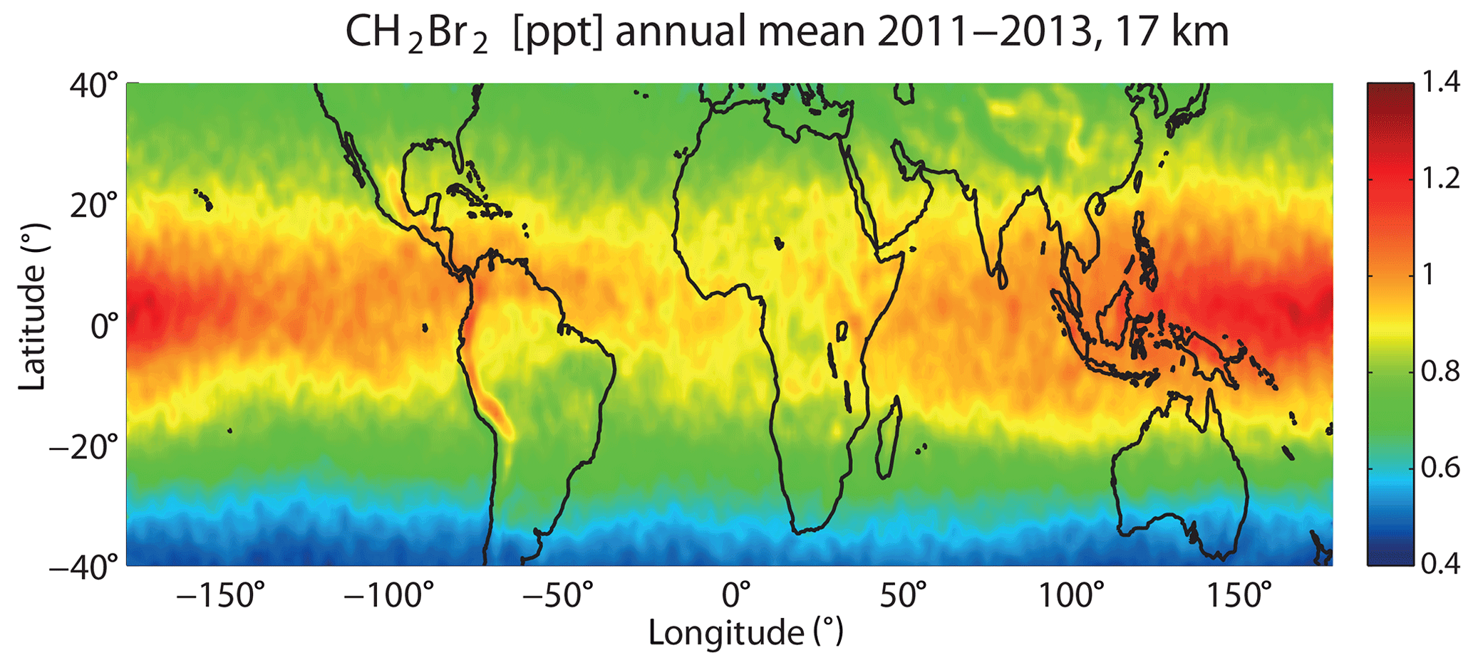
Figure 11Modelled tropical annual mean distribution of CH₂Br₂ (ppt) at 17 km for 2011–2013.

Figure 12 shows the annual tropical mean CHBr₃ and CH₂Br₂ profiles averaged over 1979–2013. At the surface, tropical mean values of 1 ppt CH₂Br₂ and 0.6 ppt CHBr₃ are simulated, which are slightly smaller than reported observations (Ziska et al., 2013, and references therein). Mixing ratios in the free troposphere decrease by nearly 50 % (10 %) for CHBr₃ (CH₂Br₂) when compared to the marine boundary layer. Both gases are well mixed in the free troposphere with nearly constant mixing ratios of 0.3 and 0.9 ppt for CHBr₃ and CH₂Br₂, respectively, corresponding to 0.9 and 1.8 ppt bromine (Fig. 12a). CHBr₃ shows a slight S shape with elevated abundances around 12–14 km related to strong convective outflow at this level bringing marine boundary layer air directly into the lower TTL. Above 14 km, CHBr₃ mixing ratios start to decrease, reaching values of 0.22 ppt at 17 km close to the cold point, corresponding to 0.66 ppt bromine. CH₂Br₂ mixing ratios, on the other hand, stay nearly constant up to 18 km, as expected based on its quite long lifetime of 400 to 500 d in the TTL, reaching values of 0.9 ppt (1.8 ppt bromine).

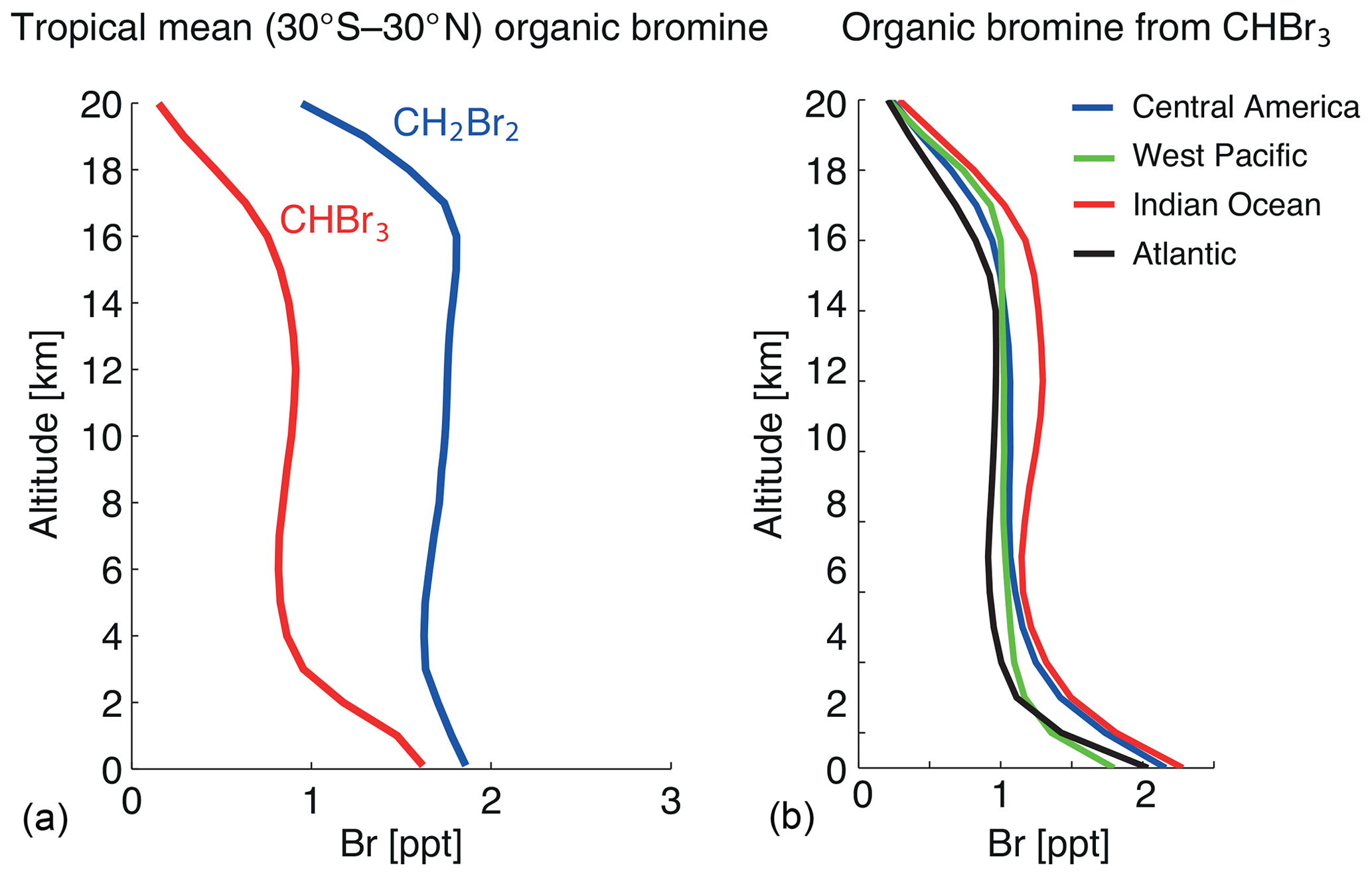
Figure 12Modelled vertical profiles of CHBr₃ and CH₂Br₂ (ppt Br) in the tropics (30^∘ S–30^∘ N) (a) and of CHBr₃ for Central America (0–20^∘ N, 70–110^∘ W), west Pacific (15^∘ S–5^∘ N, 140^∘ E–150^∘ W), Indian Ocean (0–20^∘ N, 40–110^∘ E), and Atlantic (0–20^∘ N, 20–50^∘ W) (b) for 1979–2013.

Download

CHBr₃ profiles for four different regions (Fig. 12b) show that surface atmospheric mixing ratios are strongest in the Indian Ocean and Central America. Overall, maximum mixing ratios over the Indian Ocean result from strong surface emissions combined with a relatively strong transport and main convective outflow between 11 and 14 km, giving an S-shaped CHBr₃ profile. Only for the west Pacific is transport into the stratosphere more efficient; however, smaller emissions lead to the total entrainment over this region being smaller than over the Indian Ocean.

Table 2 gives the contribution of CHBr₃ and CH₂Br₂ to the stratospheric bromine loading based on SG injection alone and based on the sum of source and PG injection. CHBr₃ and CH₂Br₂ have been evaluated directly at the cold point (as given by ERA-Interim) and contribute 2.4 ppt Br to stratospheric bromine loading directly in the form of SG entrainment with 25 % (75 %) resulting from CHBr₃ (CH₂Br₂). The CHBr₃ estimates of 0.2 ppt (corresponding to 0.6 ppt Br) are in agreement with other studies which range from 0.1 ppt (Warwick et al., 2006; Aschmann et al., 2009) to 0.35 ppt (Hossaini et al., 2012b). For CH₂Br₂, our results of 0.9 ppt (corresponding to 1.8 ppt Br) agree very well with other modelling studies (Hossaini et al., 2012b) which give estimates of 0.75–0.9 ppt. The overall contribution of the two gases in the form of SG and PG entrainment of 4.7 ppt is also in good agreement with earlier studies giving estimates ranging from 4–5 ppt (Hossaini et al., 2013) to 7.7 ppt (Liang et al., 2014).

Table 2Modelled contribution of CHBr₃ and CH₂Br₂ to the stratospheric halogen loading in the form of source gas (SG) and total (SG + PG) contribution for 2011–2013.

Download Print Version | Download XLSX

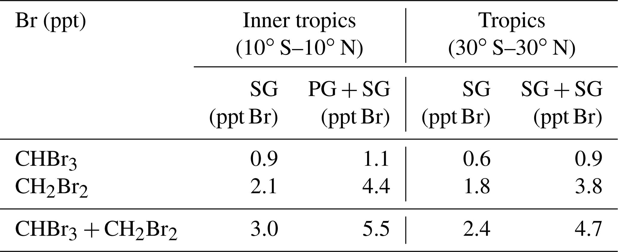
Table 3Comparison of VSLS source gas (SG) contribution derived from this study and from aircraft measurements as well as product gas (PG) contribution derived from this study and studies linking aircraft measurements and modelling.

Download Print Version | Download XLSX

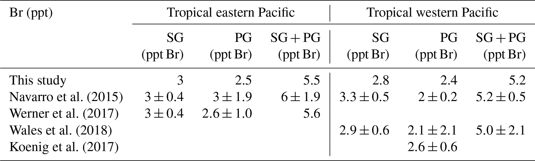
A detailed comparison of our results over the eastern and western tropical Pacific to results derived from ATTREX and CONTRAST aircraft measurements and related model calculations is given in Table 3. Considering that CHBr₃ and CH₂Br₂ contribute >80 % of the total SG Br in the TTL, our SG estimates agree very well with the measurements (Navarro et al., 2015; Werner et al., 2017; Wales et al., 2018). PG estimates are in general characterized by larger uncertainties. The PG contribution can be inferred from atmospheric measurements of BrO, the most abundant Br_y species, and the partitioning of inorganic Br_y derived from a photochemical model (Koenig et al., 2017; Werner et al., 2017; Wales et al., 2018). Uncertainties in this method arise from modelling the Br_y partitioning and from uncertainties in measuring BrO and can be as large as ±2.1 ppt (e.g. Wales et al., 2018).

Our study uses a simplified approach with a prescribed Br_y partitioning including its spatial and temporal variations. We have carried out sensitivity studies to analyse how variations in the Br_y partitioning impact the total amount of PG reaching the cold point tropopause (not shown here). Our studies show that uncertainties of 20 % in the partitioning will lead to variations of ±0.4 ppt in the PG entrainment. Such uncertainties in the Br_y partitioning can result from errors in the aerosol loading and in the heterogeneous reactions. Distributions of total Br_y and BrO in p-TOMCAT, the model used to derive the partitioning, have been shown to agree well with in situ and satellite observations (Yang et al., 2005, 2010). If the uncertainties in the partitioning would be as large as 50 %, the PG entrainment would show variations of ±1.1 ppt. Overall the PG entrainment based on our simplified approach agrees very well (within ±25 %) with estimates from other studies derived from BrO measurements and photochemical modelling (Table 3).