the Creative Commons Attribution 4.0 License.
the Creative Commons Attribution 4.0 License.
 | 15 Jun 2020
Seasonal stratospheric ozone trends over 2000–2018 derived from several merged data sets
Viktoria F. Sofieva
Doug Degenstein
Chris Roth
Sean Davis
Lucien Froidevaux
In this work, we analyze the seasonal dependence of ozone trends in the stratosphere using four long-term merged data sets, SAGE-CCI-OMPS, SAGE-OSIRIS-OMPS, GOZCARDS, and SWOOSH, which provide more than 30 years of monthly zonal mean ozone profiles in the stratosphere. We focus here on trends between 2000 and 2018. All data sets show similar results, although some discrepancies are observed. In the upper stratosphere, the trends are positive throughout all seasons and the majority of latitudes. The largest upper-stratospheric ozone trends are observed during local winter (up to 6 % per decade) and equinox (up to 3 % per decade) at mid-latitudes. In the equatorial region, we find a very strong seasonal dependence of ozone trends at all altitudes: the trends vary from positive to negative, with the sign of transition depending on altitude and season. The trends are negative in the upper-stratospheric winter (−1 % per decade to −2 % per decade) and in the lower-stratospheric spring (−2 % per decade to −4 % per decade), but positive (2 % per decade to 3 % per decade) at 30–35 km in spring, while the opposite pattern is observed in summer. The tropical trends below 25 km are negative and maximize during summer (up to −2 % per decade) and spring (up to −3 % per decade). In the lower mid-latitude stratosphere, our analysis points to a hemispheric asymmetry: during local summers and equinoxes, positive trends are observed in the south (+1 % per decade to +2 % per decade), while negative trends are observed in the north (−1 % per decade to −2 % per decade).
We compare the seasonal dependence of ozone trends with available analyses of the seasonal dependence of stratospheric temperature trends. We find that ozone and temperature trends show positive correlation in the dynamically controlled lower stratosphere and negative correlation above 30 km, where photochemistry dominates.
Seasonal trend analysis gives information beyond that contained in annual mean trends, which can be helpful in order to better understand the role of dynamical variability in short-term trends and future ozone recovery predictions.
- Article
(11426 KB) -
Supplement
(3357 KB) - BibTeX
- EndNote


The stratospheric ozone layer plays an important role in the energy budget and dynamics of the middle atmosphere by absorbing a great part of harmful ultraviolet solar radiation. Its changes in the stratosphere contribute to ground-level climate variability. International efforts by scientists and politicians resulted in the Montreal Protocol agreement and its amendments, which regulate ozone-depleting substances (ODSs). Upper-stratospheric ozone declined by about 4 % per decade to 8 % per decade in the upper stratosphere from 1980 to the late 1990s (Steinbrecht et al., 2017; WMO, 2018). The Antarctic ozone hole is showing some signs of recovery (Solomon et al., 2016), and the first signatures of global recovery have now been observed in the upper stratosphere (Bourassa et al., 2014; Kyrölä et al., 2013; Newchurch et al., 2003; Tummon et al., 2015; WMO, 2018). However, no significant trend has been detected in global total column ozone and, even though upper-stratospheric ozone is recovering, negative trends have been reported in the lower stratosphere (Ball et al., 2018; WMO, 2018). Because of the strong linkage and feedbacks between ozone depletion and climate change, continuous monitoring of ozone is very important for understanding its variability and its role in climate change. Furthermore, stratospheric ozone depletion impacts stratospheric temperature, which is also a key indicator of global climate variability. The majority of ozone trend studies have assumed that the trends can be described as a simple piecewise linear function (Bourassa et al., 2014; Kyrölä et al., 2013; Nair et al., 2015; Neu et al., 2014; Sofieva et al., 2017; Steinbrecht et al., 2017). On the other hand, more comprehensive analyses of stratospheric temperature trends have revealed large seasonal variability (Funatsu et al., 2016; Khaykin et al., 2017; Randel et al., 2016). Funatsu et al. (2016) reported cooling in the stratosphere over the period 2002–2014, at a rate of about 0.5 K per decade above 25 km. They have also shown large seasonal variability at mid-latitudes, with significant negative trends of −0.6 to −1 K per decade during summer and autumn. Khaykin et al. (2017) revealed a middle-stratospheric cooling over 2002–2016 at an average rate of −0.1 to −0.3 K per decade, with seasonal trend patterns indicating changes in the stratospheric circulation. Randel et al. (2016) have pointed to a stratospheric cooling varying from −0.1 to −0.6 K per decade over 1979–2015, with larger cooling during 1979–1997 compared to 1998–2015, mirroring the differences in upper-stratospheric ozone trends.
This paper is dedicated to an investigation of the seasonal dependence of ozone trends in the stratosphere for the post-2000 time period. For our analysis, we have used several merged satellite data sets that cover more than 3 decades (from 1984 to 2018). Ozone trends are estimated based on two-step multiple linear regression. The paper is organized as follows. Section 2 describes the merged ozone data sets. Section 3 describes the methods used for seasonal trend estimation. Section 4 describes our results regarding the seasonal dependence of ozone trends in the stratosphere. Our conclusions are summarized in Sect. 5.
In order to analyze seasonal stratospheric ozone trends, four long-term merged data sets of ozone profiles have been used.
These data sets are
- -
the SAGE-CCI-OMPS data set developed in the framework of the ESA Climate Change Initiative (Sofieva et al., 2017), referred to as CCI hereafter;
- -
SAGE-OSIRIS-OMPS developed at the University of Saskatchewan (Bourassa et al., 2014), referred to as SOO hereafter;
- -
the Global Ozone Chemistry And Related trace gas Data records for the Stratosphere (GOZCARDS) (Froidevaux et al., 2015, 2019); and
- -
the Stratospheric Water and Ozone Satellite Homogenized (SWOOSH) created by NOAA/ESRL (Davis et al., 2016).
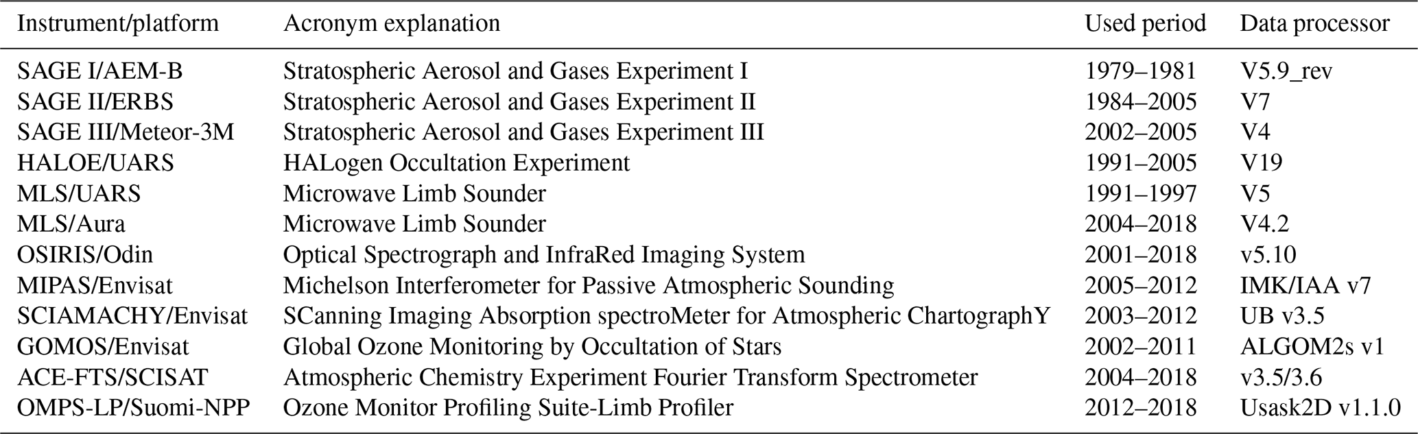
General information about the merged data sets is collected in Table 1. The basic information about individual ozone profile data sets used in the merged data sets is collected in Table 2. The collection of merged data sets represents two main groups categorized according to ozone profile representation: number density on the altitude grid (CCI and SOO) and volume mixing ratio (vmr) on the pressure grid (GOZCARDS and SWOOSH). Note that the ozone trends in different representations and vertical coordinates can be different due to temperature trends. However, since the temperature trends after 2000 are small, we expect also a minor difference in ozone trends in different ozone representations (McLinden and Fioletov, 2011). The vmr-based group uses MLS/Aura as the main data set after August 2004, while the number-density group uses other satellite instruments, with retrievals on the altitude grid, after 2005. The merged data sets use different collections of limb-profiling instruments and use different merging methods (see Table 1 and references for more details). All merged data sets are constructed from data sets with a good vertical resolution of 2–4 km. More detailed information about the merged data sets can be found in the publications mentioned above and in Table 1. All the merged data sets have been extended until December 2018. These long-term monthly zonal mean data sets cover all seasons.
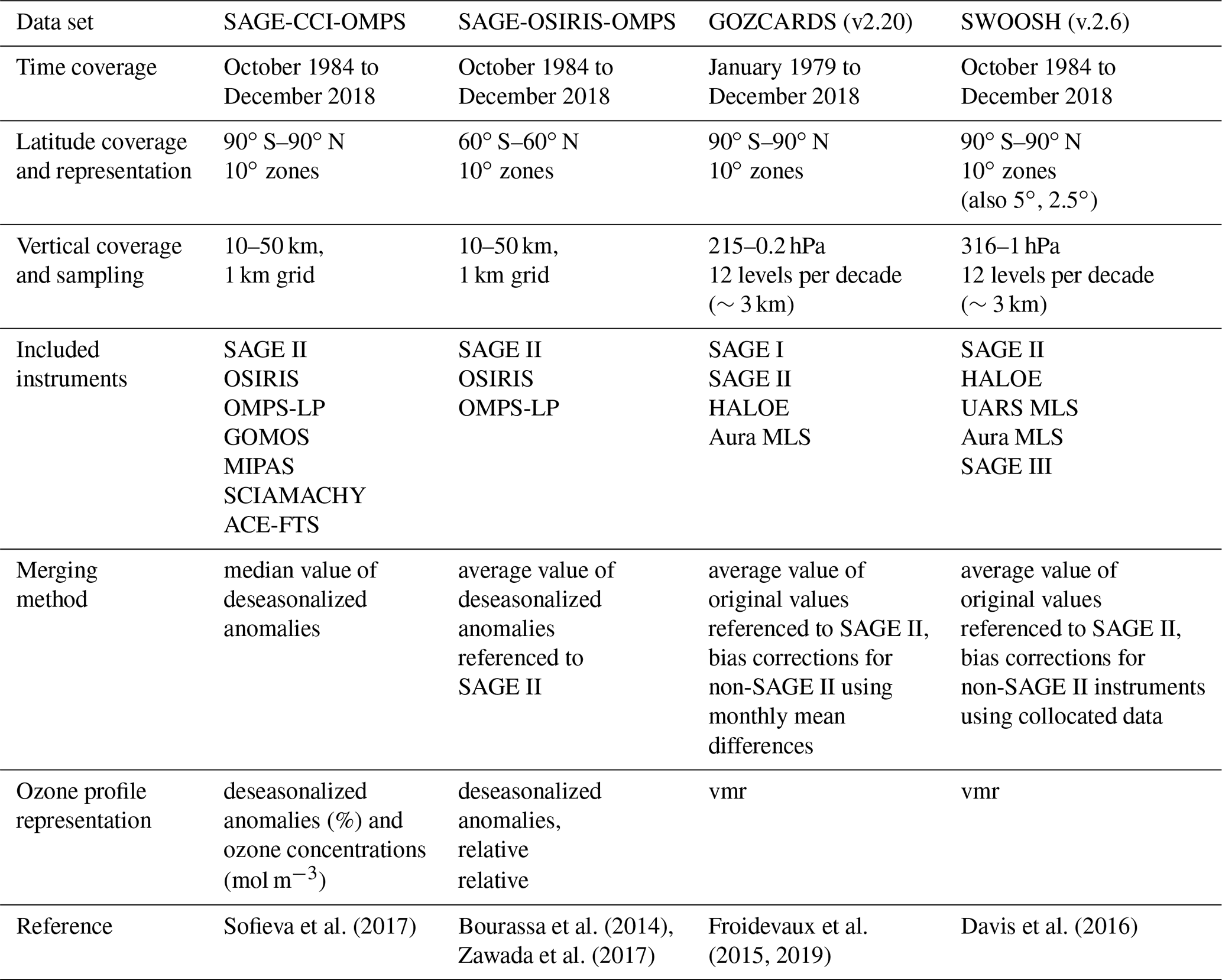
Table 2Basic information about individual satellite data sets used in the merged data sets.
The seasonal trend analysis was performed on monthly deseasonalized anomalies for all merged data sets. The CCI and SOO data sets provide deseasonalized ozone anomalies. The seasonal cycle is computed by averaging the data in each month. For GOZCARDS and SWOOSH, the deseasonalized anomalies were computed relative to their 2005–2011 mean seasonal cycle.
The trend analyses are usually performed using a multiple linear regression technique, in order to separate the natural variability and long-term trends. The known main sources of ozone variability, which are characterized by corresponding proxies, are solar cycle, quasi-biennial oscillation (QBO), and El Niño–Southern Oscillation (ENSO). In many studies, the regression is performed in one step by assuming an approximation of ozone trends by a piecewise linear function (e.g., Bourassa et al., 2014; Harris et al., 2015; Kyrölä et al., 2013; Sofieva et al., 2017). Alternatively, the regression can be performed in two steps, by detecting and removing natural cycles in the first step and estimating bulk changes over specific periods in the second step (e.g., Steinbrecht et al., 2017; WMO, 2018). This two-step approach allows us to avoid fitting over the period when the ozone trends transition from negative to positive and are not well-represented by a piecewise linear function. The two-step approach is nearly equivalent to a one-step regression, in which a piecewise linear function with three segments is fitted to the time series, as done in the SPARC LOTUS report (Petropavlovskikh et al., 2019, the independent-linear-trend, ILT, method).
Analyses of the seasonal dependence of trends are based on a smaller number of data points, compared to the traditional trend analyses, in which data from all months are used. For example, if one analyzes trends in a given month, a 30-year long data set will have only 30 data points. The fitting of all proxies in the standard multiple linear regression with insufficient data points will result in substantial uncertainty of estimated parameters. Therefore, we propose the following two-step multiple regression for seasonal trend analysis. In the first step, natural cycles are estimated from the data using the traditional multiple linear regression:
where ozone trends are approximated with a piecewise linear function (PWLT(t, t0)) with the turnaround point in 1997, QBO30(ts) and QBO50(ts) are equatorial winds at 30 and 50 hPa, respectively (http://www.cpc.ncep.noaa.gov/data/indices/, last access: 1 June 2020), F10.7(ts) is the monthly average 10.7 cm solar radio flux (ftp://ftp.geolab.nrcan.gc.ca/data/solar_flux/monthly_averages/, last access: 1 June 2020), and ENSO(ts) is the ENSO proxy (http://www.esrl.noaa.gov/psd/enso/mei/table.html, last access: 1 June 2020). The ENSO index is used with a 2-month lag, as done in several previous ozone trend analyses (e.g., Bourassa et al., 2014; Randel and Thompson, 2011; Sofieva et al., 2017). Then the fitted natural cycles are removed from the data, so only smooth variations remain in the resulting time series. The regression Eq. (1) can be performed using the data only from a certain season, usually 3 months (referred to as method no. 1 hereafter) or using data from all seasons (we will call this method no. 2). In the second step, the trends are estimated separately for the decline (1984–1997) and the recovery period (2000–2018) using a simple linear regression. In the two-step approach, a sufficient number of data points are available for detection of natural cycles – solar, QBO, and ENSO – thus providing more accurate fitting of these proxies. In the second step, fitting is only done during periods when the ozone change is approximately linear, thus avoiding the problem of modeling the ozone change in the turnaround period (such as the sensitivity to trend turnaround time when using a hockey-stick representation). Uncertainties in the second step are estimated from the fit residuals. Autocorrelations are removed in both steps using the Cochrane–Orcutt transformation (Cochrane and Orcutt, 1949).
Figure 1 illustrates each step of our analysis for the CCI data set and for two selected periods (MAM, SON) in the tropics (10∘ S–10∘ N) at altitudes between 30 and 35 km. Seasonal data (3 months, method no. 1) are used in the first step (Eq. 1). The original ozone anomalies (Fig. 1a) show a variability of about ±10 % during 1984–2018 for both seasons. The anomalies are reduced to ±6 % after the first step of the regression analysis where all proxies (QBO30, QBO50, F10.7, ENSO) are subtracted from the original data (Fig. 1b). Finally, Fig. 1c illustrates the second step of the regression analysis; i.e., linear trends are estimated for the period 2000–2018 in April (trend of +2.3 % per decade) and October (trend of −2.1 % per decade).
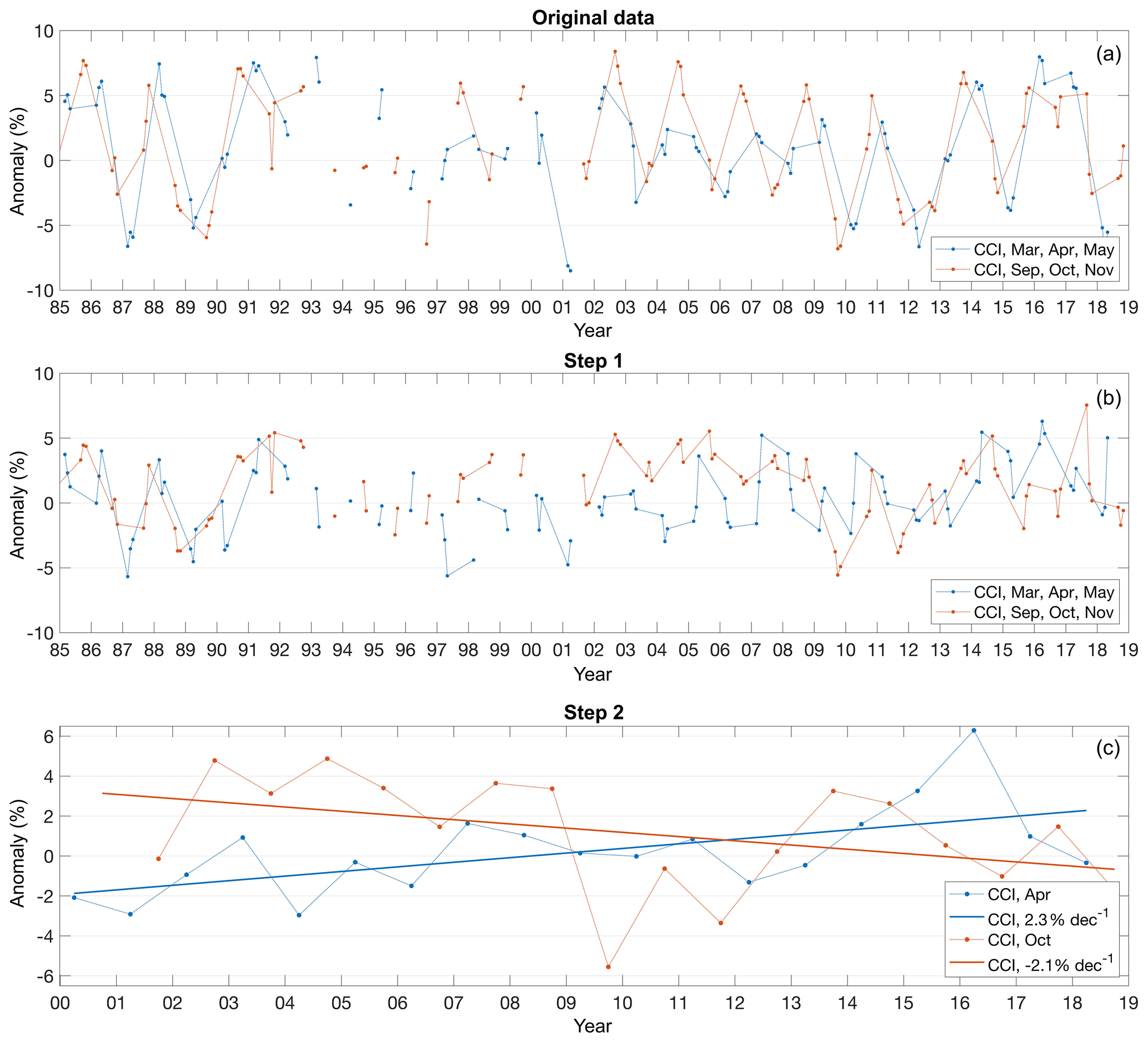
Figure 1Two-step multiple linear regression example from CCI for 10∘ S–10∘ N and 30–35 km. (a) Original ozone anomalies. (b) Anomalies with cycles removed. (c) Linear trends estimated for 2 selected months.
As described above, the amplitude of the natural cycles (solar, QBO, ENSO), which will be removed from the time series, can be estimated in two ways in the first step of our regression method, i.e., for each season separately (method no. 1) or using the data from all months, as in the traditional trend analysis (method no. 2). We have investigated both methods for estimating the natural cycles, and we found that, in general, uncertainties of method no. 1 are smaller. This is illustrated in Fig. 2, which shows the ozone trends at latitudinal bands 10∘ S–10∘ N (panels a, b) and 30–60∘ N (panels d, e) in March for these two methods. The right panels (c, f) show the differences in trends and uncertainties between both methods. At mid-latitudes, the difference in uncertainties is negligible (less than 0.3 %), but method no. 1 provides some smaller trend uncertainties, especially around ∼35 km.

Figure 2Vertical profiles of ozone trends in 2000–2018 from CCI (black), SOO (red), GOZCARDS (blue), and SWOOSH (green). The results are shown for March, latitudinal bands 10∘ S–10∘ N (a, b) and 30–60∘ N (d, e) for two separate methods (see description in the text). Error bars are 2σ uncertainties. Data are presented on their natural vertical coordinate: altitude grid (left axis) for CCI and SOO and pressure grid (right axis) for GOZCARDS and SWOOSH. Panels (c) and f) show the difference between methods for trends (solid lines) and uncertainties (dashed lines).
Such an observation is counter-intuitive: one would expect better fitting using more data points. The reason for this might be the seasonal dependence of natural cycles, particularly the QBO (Gabis et al., 2018). Assuming this, one would expect larger differences between the two methods in the tropical region, where the QBO dominates, and this is observed in Fig. 2. Although our observations – smaller residuals when fitting natural cycles using the data from a 3-month season – seem to support the hypothesis of seasonal dependence of natural cycles, this discussion is beyond the scope of our paper. From another point of view, the correlation between proxies can be different for method nos. 1 and 2; thus, the uncertainty reduction may not be fully realistic. More detailed analyses of proxy correlations can be the subject of future studies.
In the analyses shown below, we have used method no. 1 for the evaluation and removal of natural cycles. We would like to emphasize that the results are similar if method no. 2 is used (see the text below and the Supplement for details). In this work, we will focus on and discuss post-2000 trends only.
The seasonal variation of ozone trends over the 2000–2018 period as a function of latitude for five selected altitude regions is shown in Fig. 3 (colored contours). The red/blue shading (positive/negative trends) in Fig. 3 denotes trends that are statistically significant at the 95 % level.

Figure 3Latitude–season variation of linear trends in ozone for each of the merged data sets calculated over 2000–2018 for five selected altitude/pressure ranges. The shading denotes trends that are significant at the 95 % level. Pressure ranges correspond approximately to altitude ranges.
In the tropical region (20∘ S–20∘ N), a strong seasonal dependence of ozone trends is observed. In the lower stratosphere (19–23 km), the pattern of statistically significant negative trends of about −2 % per decade to −3 % per decade is present in all merged data sets during the spring and summer months (MAM and JJA), while they are less pronounced in other months. At altitudes 24–28 km, the trends change from negative (−1 % per decade to −2 % per decade, statistically significant for all except SOO) in spring (MAM) to positive (+1 % per decade to +2 % per decade, statistically significant for CCI and SOO) in autumn (SON). At 31–35 km in the tropics, the trends are opposite: positive trends in MAM (+2 % per decade to +3 % per decade, statistically significant) and negative in SON (−1 % per decade to −2 % per decade, not statistically significant).
Above 40 km, trends are in general positive throughout the latitudes and months, with the largest trends observed at mid-latitudes (30–60∘ N/S) during the local winters and spring/autumn seasons (2 % per decade to 4 % per decade). Upper-stratospheric recovery for all latitude bands has been obtained by others (e.g., Petropavlovskikh et al., 2019; Steinbrecht et al., 2017; WMO, 2018); nonetheless, for seasonal analysis, negative trends of −1 % per decade to −2 % per decade during the late winter (DJF) are present in the tropics, although with statistical significance only in the CCI data sets.
Analysis results from broader latitude bands are presented in Fig. 4 (method no. 1) and Fig. S1 in the Supplement (method no. 2). Both methods as well as all data sets generally show very similar results. The uncertainties of method no. 1 are usually smaller than for method no. 2, which makes the observed patterns more statistically significant. The basic structure and patterns of seasonal trends are apparent in the monthly data as well (Figs. S2 and S3), but the magnitude of the calculated trends is higher for each single month.

Figure 4Altitude–season variation of linear trends in ozone for each of the merged data sets calculated over 2000–2018 for three selected latitudinal bands. Data are presented on their natural vertical coordinate: altitude grid for CCI and SOO and pressure grid for GOZCARDS and SWOOSH. The shading denotes trends that are significant at the 95 % level.
Figure 4 reveals negative trends ranging from −1 % per decade to −2 % per decade in the lower/middle stratosphere at 30–60∘ N during the summer (JJA). Negative trends are present in all data sets and are statistically significant for all except the CCI data set. In contrast, in the lower/middle southern stratosphere (30–60∘ S), trends are positive (1 % per decade to 2 % per decade) and statistically significant for all data sets.
In the equatorial region, all data sets show pronounced, statistically significant, and very similar seasonal dependence of ozone trends. In the upper tropical stratosphere above 40 km, trends are negative in DJF (−1 % per decade to −3 % per decade, significant for all except SOO) and positive in August–October (2 %–3 %, statistically significant for all data sets). At 30–35 km, trends are positive in MAM at altitudes 30–35 km (2 % per decade to 3 % per decade, significant for all) and negative in SON ( % per decade, statistically significant for CCI and SOO). In the lower stratosphere, the negative trends are in MAM (−2 % per decade to −3 % per decade, significant for all) and positive in DJF (1 % to 2 % per decade, significant for CCI and SOO).
Upper-stratospheric trends at mid-latitudes are most pronounced during the local winters and equinoxes, varying from 3 % per decade to 4 % per decade in the north and from 2 % per decade to 3 % per decade in the south.
All merged ozone data sets show a similar seasonal dependence of the ozone trends. Some difference in ozone trends can also be due to the differing vertical grids used in the various data sets. To estimate this, we have calculated the seasonal trends for “number density on altitude grid” (CCI, SOO) and also for “vmr on pressure grid” (GOZCARDS, SWOOSH), as shown in Fig. S4. The estimated difference is consistent with the pattern of temperature trends and predictions by McLinden and Fioletov (2011).
Figure 5 shows the seasonal ozone trends (color) together with yearly trend (black) plotted in the vertical distribution for three selected latitudinal bands. It is clear that at mid-latitudes, positive trends in the upper stratosphere are dominant in the local winters (up to 4 % per decade) and are much higher than the yearly trend (up to 2 % per decade). In the tropics, the main features observed during different seasons (i.e., negative–positive patterns observed throughout the seasons and vertical levels) mostly cancel out in the yearly trend. Negative winter trends (DJF) in the upper stratosphere (−3 % per decade), negative spring trends (MAM) in the lower stratosphere (−3 % per decade to −4 % per decade), and positive spring trends (MAM) in the middle stratosphere (2 % per decade) are all counterbalanced by opposite or smaller trends during the remaining seasons. As a result, the yearly ozone trend in the tropics is much smaller than the seasonal trends. The other data sets show consistently similar features (Fig. S5). The main discrepancies are observed between number density-based group (SOO and CCI) and vmr-based group (GOZCARDS and SWOOSH) during summer (JJA) in the upper stratosphere in the south.

Figure 5Vertical profiles of seasonal (red, blue, green, magenta) and yearly (black) ozone trends in 2000–2018 from SWOOSH. The results are shown for three selected latitude bands. Error bars and shaded area (gray) are 2σ uncertainties.
To summarize our analysis, variations of ozone trends over the period 2000–2018 for each latitude and vertical level are plotted for each season separately in Fig. 6.
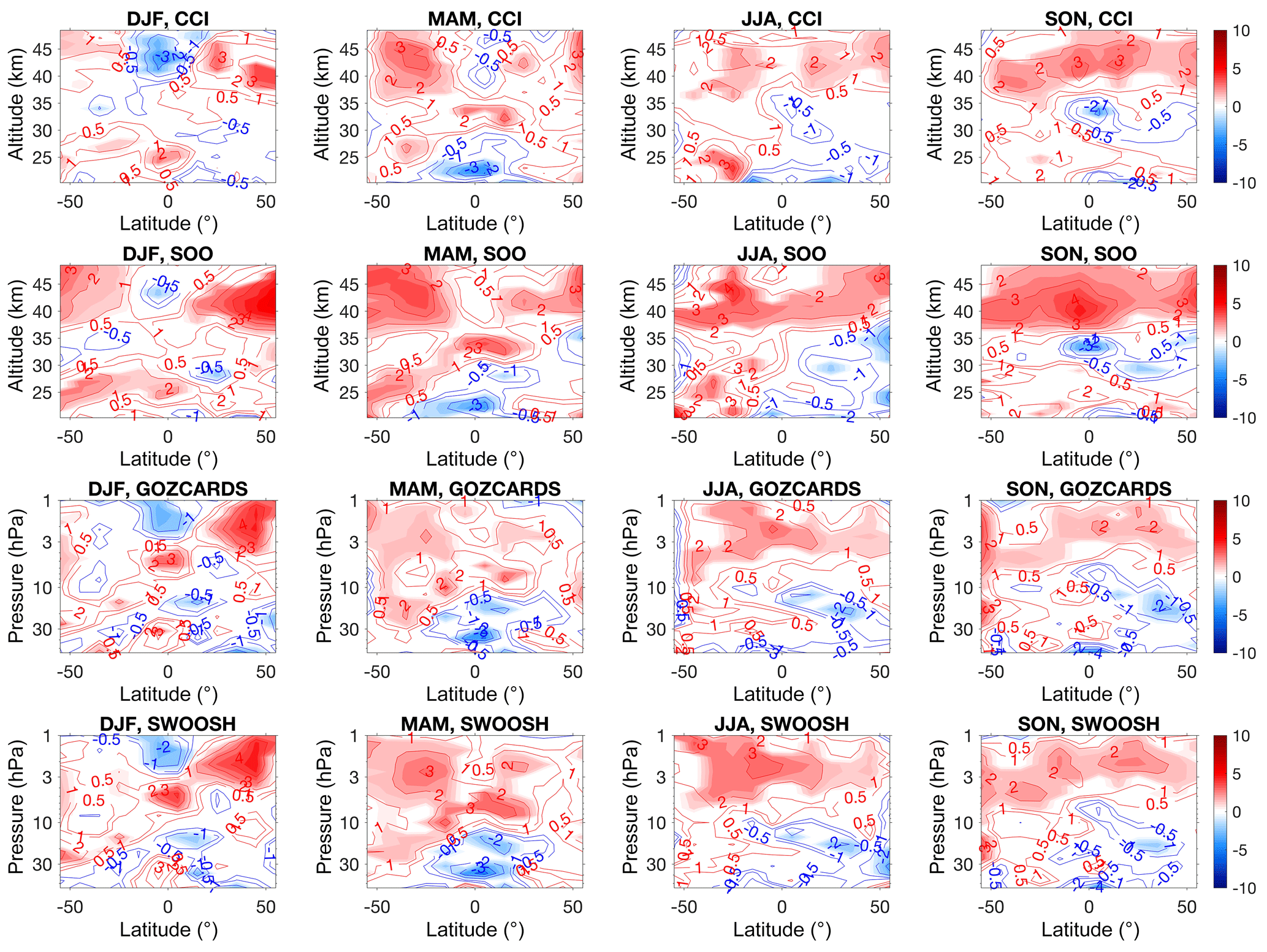
Figure 6Altitude–latitude variation of linear trends in ozone calculated over 2000–2018 for each season. Data are presented on their natural vertical coordinate: altitude grid for CCI and SOO and pressure grid for GOZCARDS and SWOOSH. The shading denotes trends that are significant at the 95 % level.
In the upper stratosphere, trends are positive throughout all seasons and the majority of latitudes. One of the most pronounced features is that the mid-latitude upper-stratospheric ozone trends are larger in local winters. As discussed in Sect. 1, ozone and temperature trends are inter-related, as ozone and temperature are connected via photochemical reactions, effective above ∼25–30 km (Brasseur and Solomon, 2005). Randel et al. (2016) reported weaker upper-stratospheric cooling in local winter at mid-latitudes and high latitudes. This is fully consistent with our observations of larger positive ozone trends at these locations in winter. A hypothesized explanation of this feature might be the acceleration of the upper branch of the Brewer–Dobson circulation (or in general mean residual circulation), which controls the meridional transport of trace gases from the tropical region to the poles (Brewer, 1949; Dobson, 1956). The Brewer–Dobson circulation (BDC) is most effective during the winter season (Chipperfield and Jones, 1999). Several modeling studies have shown that due to greenhouse gas concentration (GHG) increases, the wintertime BDC will strengthen and accelerate the expected ozone recovery (Butchart et al., 2006; Garcia and Randel, 2008; Gettelman et al., 2010; Li et al., 2008; Schnadt et al., 2002; Sigmond et al., 2004). Also, observational studies have shown an accelerated BDC over the tropical region (Thompson and Solomon, 2009) as well as at high latitudes (Hu and Fu, 2009). Increased speed of the BDC would have an effect on the transport of ozone and ODSs. While the main reason for positive ozone trends in the upper mid-latitude stratosphere is the decrease in ozone-depleting substances, the seasonal variations of the ozone trends can be due to dynamics. Seasonal dependence of both temperature and ozone trends supports this hypothesis. However, the investigation of the mechanisms that control the seasonality of ozone and temperature trends is beyond the scope of our paper; it can be the subject of future modeling and observational studies.
In the tropics, our analysis has shown a very strong seasonal dependence of ozone trends observed at all altitudes. The trends change from positive to negative, with the phase changing with altitude. In the tropical lower stratosphere below 25 km, strong negative trends are observed during boreal spring and summer, which are statistically significant for all data sets. Khaykin et al. (2017) also found an altitude-dependent pattern in temperature trends in the tropical region, with a strong seasonality. One can notice that the changes in phases in ozone and temperature trends are very similar (temperature trends are evaluated below 35 km in Khaykin et al., 2017). In the lower tropical stratosphere, in the dynamically controlled region, ozone and temperature variations are positively correlated (Hauchecorne et al., 2010), as are the ozone and temperature trends (compare our Fig. 8 with Fig. 5 in Khaykin et al., 2017). This is rather expected and can serve as additional confirmation of our hypotheses explaining this seasonality. Khaykin et al. (2017) hypothesized that the observed trend structure might be related to seasonal variations in the Brewer–Dobson circulation.
The third interesting feature is hemispheric asymmetry of summertime ozone trend patterns below 35 km: they are negative in the Northern Hemisphere (NH) and positive in the Southern Hemisphere (SH). No similar analyses exist for temperature, and this can be the subject of future work. Hemispheric asymmetry was reported in recent studies (Froidevaux et al., 2019; Ball et al., 2019), even if not broken down by season. Froidevaux et al. (2019) showed that ozone trends derived from Aura Microwave Limb Sounder (Aura/MLS) data over a shorter period (2005–2018) have a tendency towards slightly positive values in the SH. Additionally, this asymmetry might be related to the hydrogen chloride (HCl) abundances and trends (Mahieu et al., 2014; Han et al., 2019). At the moment, we can only speculate that this might also be a contributing factor to the observed ozone negative trends in that region.
Using four long-term merged data sets of ozone profiles, we have studied the seasonal dependence of ozone trends in the stratosphere. The results of our analysis, based on two-step multiple linear regression, can be summarized as follows.
- -
The upper-stratospheric ozone is recovering, and the recovery maximizes during local winters and equinoxes, reaching up to 3 % per decade to 4 % per decade, which is fully consistent with weaker upper-stratospheric cooling in local winter at mid-latitudes and high latitudes.
- -
In the tropics, there is very strong seasonal dependence of ozone trends at all altitudes. The trends are changing from positive to negative, with the sign of transition depending on altitude and season.
- -
Below 25 km in the tropical region, strong negative trends are observed during spring and summer, which are statistically significant for all data sets and consistent with the seasonal pattern of temperature trends in this region.
- -
In the lower and middle stratosphere, there is hemispheric asymmetry during the local summers and equinoxes at mid-latitudes, with a negative trend in the north and a positive trend in the south.
Despite some discrepancies, the general coherence in trends derived from four different merged data sets gives us confidence in the validity and robustness of the results. We compared the seasonal dependence of ozone trends with available analyses of the seasonal dependence of stratospheric temperature trends and found a clear inter-relation of the trend patterns.
The SAGE-CCI-OMPS data set is available from the CCI website (http://www.esa-ozone-cci.org, last access:1 June 2020, ESA, 2020). The SAGEII-OSIRIS-OMPS data set is available from the University of Saskatchewan ftp site. GOZCARDS ozone data updates (version 2.20) are available by contacting Lucien Froidevaux; this data version will also be updated on the public Goddard Earth Sciences Data and Information Services Center (GES DISC) website (https://disc.gsfc.nasa.gov, last access: 1 June 2020, NASA, 2020) in the near future.
The supplement related to this article is available online at: https://doi.org/10.5194/acp-20-7035-2020-supplement.
MES and VFS designed the study, performed analysis and wrote the manuscript. DD, CR, SD and LF provided the dataset and contributed to the analysis and writing of the manuscript.
The authors declare that they have no conflict of interest.
The SAGE-CCI-OMPS data set was created within the ESA Ozone_CCI project. Viktoria F. Sofieva and Monika E. Szeląg thank the Academy of Finland (projects INQUIRE and SECTIC, Center of Excellence of Inverse Modelling and Imaging). The authors thank the Canadian Space Agency. Work at the Jet Propulsion Laboratory, California Institute of Technology, was performed under contract with the National Aeronautics and Space Administration (NASA). We acknowledge the essential contributions from Ray Wang, John Anderson and Ryan Fuller to the GOZCARDS data records used here.
This paper was edited by Michel Van Roozendael and reviewed by two anonymous referees.
Ball, W. T., Alsing, J., Mortlock, D. J., Staehelin, J., Haigh, J. D., Peter, T., Tummon, F., Stübi, R., Stenke, A., Anderson, J., Bourassa, A., Davis, S. M., Degenstein, D., Frith, S., Froidevaux, L., Roth, C., Sofieva, V., Wang, R., Wild, J., Yu, P., Ziemke, J. R., and Rozanov, E. V.: Evidence for a continuous decline in lower stratospheric ozone offsetting ozone layer recovery, Atmos. Chem. Phys., 18, 1379–1394, https://doi.org/10.5194/acp-18-1379-2018, 2018.
Ball, W. T., Chiodo, G., Abalos, M., and Alsing, J.: Inconsistencies between chemistry climate model and observed lower stratospheric trends since 1998, Atmos. Chem. Phys. Discuss., https://doi.org/10.5194/acp-2019-734, in review, 2019.
Bourassa, A. E., Degenstein, D. A., Randel, W. J., Zawodny, J. M., Kyrölä, E., McLinden, C. A., Sioris, C. E., and Roth, C. Z.: Trends in stratospheric ozone derived from merged SAGE II and Odin-OSIRIS satellite observations, Atmos. Chem. Phys., 14, 6983–6994, https://doi.org/10.5194/acp-14-6983-2014, 2014.
Brasseur, G. P. and Solomon, S.: Aeronomy of the Middle Atmosphere, 3rd edn., D. Reidel Publishing Company, Dordrecht, 2005.
Brewer, A. W.: Evidence for a world circulation provided by the measurements of helium and water vapor distribution in the stratosphere, Q. J. Roy. Meteor. Soc., 75, 351–363, 1949.
Butchart, N., Scaife, A. A., Bourqui, M., Grandpré, J., Hare, S. H. E., Kettleborough, J., Langematz, U., Manzini, E., Sassi, F., Shibata, K., Shindell, D., and Sigmond, M.: Simulations of anthropogenic change in the strength of the Brewer-Dobson circulation, Clim. Dynam., 27, 727–741, https://doi.org/10.1007/s00382-006-0162-4, 2006.
Chipperfield, M. P. and Jones, R. L.: Relative influences of atmospheric chemistry and transport on Arctic ozone trends, Nature, 400, 3–6, 1999.
Cochrane, D. and Orcutt, G. H.: Application of Least Squares Regression to Relationships Containing Auto-Correlated Error Terms, J. Am. Stat. Assoc., 44, 32–61, https://doi.org/10.1080/01621459.1949.10483290, 1949.
Davis, S. M., Rosenlof, K. H., Hassler, B., Hurst, D. F., Read, W. G., Vömel, H., Selkirk, H., Fujiwara, M., and Damadeo, R.: The Stratospheric Water and Ozone Satellite Homogenized (SWOOSH) database: a long-term database for climate studies, Earth Syst. Sci. Data, 8, 461–490, https://doi.org/10.5194/essd-8-461-2016, 2016.
Dobson, G. M. B.: Origin and distribution of polyatomic molecules in the atmosphere, P. Roy. Soc. A-Math. Phy., 236, 187–193, 1956.
ESA: Climate Change Initiative (CCI), available at: http://www.esa-ozone-cci.org, last access: 1 June 2020.
Froidevaux, L., Anderson, J., Wang, H.-J., Fuller, R. A., Schwartz, M. J., Santee, M. L., Livesey, N. J., Pumphrey, H. C., Bernath, P. F., Russell III, J. M., and McCormick, M. P.: Global OZone Chemistry And Related trace gas Data records for the Stratosphere (GOZCARDS): methodology and sample results with a focus on HCl, H2O, and O3, Atmos. Chem. Phys., 15, 10471–10507, https://doi.org/10.5194/acp-15-10471-2015, 2015.
Froidevaux, L., Kinnison, D. E., Wang, R., Anderson, J., and Fuller, R. A.: Evaluation of CESM1 (WACCM) free-running and specified dynamics atmospheric composition simulations using global multispecies satellite data records, Atmos. Chem. Phys., 19, 4783–4821, https://doi.org/10.5194/acp-19-4783-2019, 2019.
Funatsu, B. M., Claud, C., Keckhut, P., Hauchecorne, A., and Leblanc, T.: Regional and seasonal stratospheric temperature trends in the last decade (2002–2014) from AMSU observations, J. Geophys. Res., 121, 8172–8185, https://doi.org/10.1002/2015JD024305, 2016.
Gabis, I. P.: Seasonal dependence of the quasi-biennial oscillation (QBO): New evidence from IGRA data, J. Atmos. Sol.-Terr. Phy., 179, 316–336, https://doi.org/10.1016/j.jastp.2018.08.012, 2018
Garcia, R. R. and Randel, W. J.: Acceleration of the Brewer–Dobson circulation due to increases in greenhouse gases, J. Atmos. Sci., 65, 2731–2739, https://doi.org/10.1175/2008JAS2712.1, 2008.
Gettelman, A., Hegglin, M. I., Son, S.-W., Kim, J., Fujiwara, M., Birner, T., Kremser, S., Rex, M., Añel, J. A., Akiyoshi, H., Austin, J., Bekki, S., Braesike, P., Brühl, C., Butchart, N., Chipperfield, M., Dameris, M., Dhomse, S., Garny, H., Hardiman, S. C., Jöckel, P., Kinnison, D. E., Lamarque, J. F., Mancini, E., Marchand, M., Michou, M., Morgenstern, O., Pawson, S., Pitari, G., Plummer, D., Pyle, J. A., Rozanov, E., Scinocca, J., Shepherd, T. G., Shibata, K., Smale, D., Teyssèdre, H., and Tian, W.: Multimodel assessment of the upper troposphere and lower stratosphere: Tropics and global trends, J. Geophys. Res. Atmos., 115, D00M08, https://doi.org/10.1029/2009JD013638, 2010.
Han, Y., Tian, W., Chipperfield, M. P., Zhang, J., Wang, F., Sang, W., Luo, J., Feng, W., Chrysanthou, A., and Tian, H.: Attribution of the hemispheric asymmetries in trends of stratospheric trace gases inferred from Microwave Limb Sounder (MLS) measurements, J. Geophys. Res.-Atmos., 124, 6283–6293, https://doi.org/10.1029/2018JD029723, 2019.
Harris, N. R. P., Hassler, B., Tummon, F., Bodeker, G. E., Hubert, D., Petropavlovskikh, I., Steinbrecht, W., Anderson, J., Bhartia, P. K., Boone, C. D., Bourassa, A., Davis, S. M., Degenstein, D., Delcloo, A., Frith, S. M., Froidevaux, L., Godin-Beekmann, S., Jones, N., Kurylo, M. J., Kyrölä, E., Laine, M., Leblanc, S. T., Lambert, J.-C., Liley, B., Mahieu, E., Maycock, A., de Mazière, M., Parrish, A., Querel, R., Rosenlof, K. H., Roth, C., Sioris, C., Staehelin, J., Stolarski, R. S., Stübi, R., Tamminen, J., Vigouroux, C., Walker, K. A., Wang, H. J., Wild, J., and Zawodny, J. M.: Past changes in the vertical distribution of ozone – Part 3: Analysis and interpretation of trends, Atmos. Chem. Phys., 15, 9965–9982, https://doi.org/10.5194/acp-15-9965-2015, 2015.
Hauchecorne, A., Bertaux, J. L., Dalaudier, F., Keckhut, P., Lemennais, P., Bekki, S., Marchand, M., Lebrun, J. C., Kyrölä, E., Tamminen, J., Sofieva, V., Fussen, D., Vanhellemont, F., Fanton d'Andon, O., Barrot, G., Blanot, L., Fehr, T., and Saavedra de Miguel, L.: Response of tropical stratospheric O3, NO2 and NO3 to the equatorial Quasi-Biennial Oscillation and to temperature as seen from GOMOS/ENVISAT, Atmos. Chem. Phys., 10, 8873–8879, https://doi.org/10.5194/acp-10-8873-2010, 2010.
Hu, Y. and Fu, Q.: Stratospheric warming in Southern Hemisphere high latitudes since 1979, Atmos. Chem. Phys., 9, 4329–4340, https://doi.org/10.5194/acp-9-4329-2009, 2009.
Khaykin, S. M., Funatsu, B. M., Hauchecorne, A., Godin-Beekmann, S., Claud, C., Keckhut, P., Pazmino, A., Gleisner, H., Nielsen, J. K., Syndergaard, S., and Lauritsen, K. B.: Postmillennium changes in stratospheric temperature consistently resolved by GPS radio occultation and AMSU observations, Geophys. Res. Lett., 44, 7510–7518, https://doi.org/10.1002/2017GL074353, 2017.
Kyrölä, E., Laine, M., Sofieva, V., Tamminen, J., Päivärinta, S.-M., Tukiainen, S., Zawodny, J., and Thomason, L.: Combined SAGE II–GOMOS ozone profile data set for 1984–2011 and trend analysis of the vertical distribution of ozone, Atmos. Chem. Phys., 13, 10645–10658, https://doi.org/10.5194/acp-13-10645-2013, 2013.
Li, F., Austin, J., and Wilson, J.: The strength of the Brewer-Dobson circulation in a changing climate: Coupled chemistry-climate model simulations, J. Climate, 21, 40–57, https://doi.org/10.1175/2007JCLI1663.1, 2008.
Mahieu, E., Chipperfield, M. P., Notholt, J., Reddmann, T., Anderson, J., Bernath, P. F., Blumenstock, T., Coffey, M. T., Dhomse, S. S., Feng, W., Franco, B., Froidevaux, L., Griffith, D. W. T., Hannigan, J. W., Hase, F., Hossaini, R., Jones, N. B., Morino, I., Murata, I., Nakajima, H., Palm, M., Paton-Walsh, C., Russell, J. M., Schneider, M., Servais, C., Smale, D., and Walker, K. A.: Recent Northern Hemisphere stratospheric HCl increase due to atmospheric circulation changes, Nature, 515, 104–107, https://doi.org/10.1038/nature13857, 2014.
McLinden, C. A. and Fioletov, V.: Quantifying trends in stratospheric ozone: Complications due to stratospheric cooling, Geophys. Res. Lett., 38, L03808, https://doi.org/10.1029/2010GL046012, 2011.
Nair, P. J., Froidevaux, L., Kuttippurath, J., Zawodny, J. M., Russell, J. M., Steinbrecht, W., Claude, H., Leblanc, T., van Gijsel, J. A. E., Johnson, B., Swart, D. P. J., Thomas, A., Querel, R., Wang, R., and Anderson, J.: Subtropical and midlatitude ozone trends in the stratosphere: Implications for recovery, J. Geophys. Res., 120, 7247–7257, https://doi.org/10.1002/2014JD022371, 2015.
NASA: GES DISC, available at: https://disc.gsfc.nasa.gov, last access: 1 June 2020.
Neu, J. L., Hegglin, M. I., Tegtmeier, S., Bourassa, A., Degenstein, D., Froidevaux, L., Fuller, R., Funke, B., Gille, J., Jones, A., Rozanov, A., Toohey, M., von Clarmann, T., Walker, K. A., and Worden, J. R.: The SPARC Data Initiative: Comparison of upper troposphere/lower stratosphere ozone climatologies from limb-viewing instruments and the nadir-viewing Tropospheric Emission Spectrometer, J. Geophys. Res.-Atmos., 119, 6971–6990, https://doi.org/10.1002/2013JD020822, 2014.
Newchurch, M. J., Yang, E.-S., Cunnold, D. M., Reinsel, G. C., Zawodny, J. M., and Russell, J. M.: Evidence for slowdown in stratospheric ozone loss: First stage of ozone recovery, J. Geophys. Res., 108, 4507, https://doi.org/10.1029/2003JD003471, 2003.
Petropavlovskikh, I., Godin-Beekmann, S., Hubert, D., Damadeo, R., Hassler, B., and Sofieva, V.: SPARC/IO3C/GAW Report on Long-term Ozone Trends and Uncertainties in the Stratosphere, edited by: Kenntner, M. and Ziegele, B., SPARC Report No. 9, GAW Report No. 241, WCRP Report 17/2018, https://doi.org/10.17874/f899e57a20b, 2019.
Randel, W. J. and Thompson, A. M.: Interannual variability and trends in tropical ozone derived from SAGE II satellite data and SHADOZ ozonesondes, J. Geophys. Res., 116, D07303, https://doi.org/10.1029/2010JD015195, 2011.
Randel, W. J., Smith, A. K., Wu, F., Zou, C. Z., and Qian, H.: Stratospheric temperature trends over 1979–2015 derived from combined SSU, MLS, and SABER satellite observations, J. Climate, 29, 4843–4859, https://doi.org/10.1175/JCLI-D-15-0629.1, 2016.
Schnadt, C., Dameris, M., Ponater, M., Hein, R., Grewe, V., and Steil, B.: Interaction of atmospheric chemistry and climate and its impact on stratospheric ozone, Clim. Dynam., 18, 501–517, https://doi.org/10.1007/s00382-001-0190-z, 2002.
Sigmond, M., Siegmund, P. C., Manzini, E., and Kelder, H.: A simulation of the separate climate effects of middle-atmospheric and tropospheric CO2 doubling, J. Climate, 17, 2352–2367, https://doi.org/10.1175/1520-0442(2004)017<2352:ASOTSC>2.0.CO;2, 2004.
Sofieva, V. F., Kyrölä, E., Laine, M., Tamminen, J., Degenstein, D., Bourassa, A., Roth, C., Zawada, D., Weber, M., Rozanov, A., Rahpoe, N., Stiller, G., Laeng, A., von Clarmann, T., Walker, K. A., Sheese, P., Hubert, D., van Roozendael, M., Zehner, C., Damadeo, R., Zawodny, J., Kramarova, N., and Bhartia, P. K.: Merged SAGE II, Ozone_cci and OMPS ozone profile dataset and evaluation of ozone trends in the stratosphere, Atmos. Chem. Phys., 17, 12533–12552, https://doi.org/10.5194/acp-17-12533-2017, 2017.
Solomon, S., Ivy, D. J., Kinnison, D., Mills, M. J., Neely III, R. R., and Schmidt, A.: Emergence of healing in the Antarctic ozone layer, Science, 353, 269–274, https://doi.org/10.1126/science.aae0061, 2016
Steinbrecht, W., Froidevaux, L., Fuller, R., Wang, R., Anderson, J., Roth, C., Bourassa, A., Degenstein, D., Damadeo, R., Zawodny, J., Frith, S., McPeters, R., Bhartia, P., Wild, J., Long, C., Davis, S., Rosenlof, K., Sofieva, V., Walker, K., Rahpoe, N., Rozanov, A., Weber, M., Laeng, A., von Clarmann, T., Stiller, G., Kramarova, N., Godin-Beekmann, S., Leblanc, T., Querel, R., Swart, D., Boyd, I., Hocke, K., Kämpfer, N., Maillard Barras, E., Moreira, L., Nedoluha, G., Vigouroux, C., Blumenstock, T., Schneider, M., García, O., Jones, N., Mahieu, E., Smale, D., Kotkamp, M., Robinson, J., Petropavlovskikh, I., Harris, N., Hassler, B., Hubert, D., and Tummon, F.: An update on ozone profile trends for the period 2000 to 2016, Atmos. Chem. Phys., 17, 10675–10690, https://doi.org/10.5194/acp-17-10675-2017, 2017.
Thompson, D. W. J. and Solomon, S.: Understanding recent stratospheric climate change, J. Climate, 22, 1934–1943, https://doi.org/10.1175/2008JCLI2482.1, 2009.
Tummon, F., Hassler, B., Harris, N. R. P., Staehelin, J., Steinbrecht, W., Anderson, J., Bodeker, G. E., Bourassa, A., Davis, S. M., Degenstein, D., Frith, S. M., Froidevaux, L., Kyrölä, E., Laine, M., Long, C., Penckwitt, A. A., Sioris, C. E., Rosenlof, K. H., Roth, C., Wang, H.-J., and Wild, J.: Intercomparison of vertically resolved merged satellite ozone data sets: interannual variability and long-term trends, Atmos. Chem. Phys., 15, 3021–3043, https://doi.org/10.5194/acp-15-3021-2015, 2015.
WMO: Scientific Assessment of Ozone Depletion: 2018, Global Ozone Research and Monitoring Project, Report No. 58, 590 pp., Geneva, Switzerland, 2018.
Zawada, D. J., Rieger, L. A., Bourassa, A. E., and Degenstein, D. A.: Tomographic retrievals of ozone with the OMPS Limb Profiler: algorithm description and preliminary results, Atmos. Meas. Tech., 11, 2375–2393, https://doi.org/10.5194/amt-11-2375-2018, 2018.