the Creative Commons Attribution 4.0 License.
the Creative Commons Attribution 4.0 License.
 | 12 Jun 2020
Quantifying uncertainties of climate signals in chemistry climate models related to the 11-year solar cycle – Part 1: Annual mean response in heating rates, temperature, and ozone
Markus Kunze
Tim Kruschke
Ulrike Langematz
Miriam Sinnhuber
Thomas Reddmann
Katja Matthes
Variations in the solar spectral irradiance (SSI) with the 11-year sunspot cycle have been shown to have a significant impact on temperatures and the mixing ratios of atmospheric constituents in the stratosphere and mesosphere. Uncertainties in modelling the effects of SSI variations arise from uncertainties in the empirical models reconstructing the prescribed SSI data set as well as from uncertainties in the chemistry–climate model (CCM) formulation. In this study CCM simulations with the ECHAM/MESSy Atmospheric Chemistry (EMAC) model and the Community Earth System Model 1 (CESM1)–Whole Atmosphere Chemistry Climate Model (WACCM) have been performed to quantify the uncertainties of the solar responses in chemistry and dynamics that are due to the usage of five different SSI data sets or the two CCMs. We apply a two-way analysis of variance (ANOVA) to separate the influence of the SSI data sets and the CCMs on the variability of the solar response in shortwave heating rates, temperature, and ozone. The solar response is derived from climatological differences of time slice simulations prescribing SSI for the solar maximum in 1989 and near the solar minimum in 1994. The SSI values for the solar maximum of each SSI data set are created by adding the SSI differences between November 1994 and November 1989 to a common SSI reference spectrum for near-solar-minimum conditions based on ATLAS-3 (Atmospheric Laboratory of Applications and Science-3). The ANOVA identifies the SSI data set with the strongest influence on the variability of the solar response in shortwave heating rates in the upper mesosphere and in the upper stratosphere–lower mesosphere. The strongest influence on the variability of the solar response in ozone and temperature is identified in the upper stratosphere–lower mesosphere. However, in the region of the largest ozone mixing ratio, in the stratosphere from 50 to 10 hPa, the SSI data sets do not contribute much to the variability of the solar response when the Spectral And Total Irradiance REconstructions-T (SATIRE-T) SSI data set is omitted. The largest influence of the CCMs on variability of the solar responses can be identified in the upper mesosphere. The solar response in the lower stratosphere also depends on the CCM used, especially in the tropics and northern hemispheric subtropics and mid-latitudes, where the model dynamics modulate the solar responses. Apart from the upper mesosphere, there are also regions where the largest fraction of the variability of the solar response is explained by randomness, especially for the solar response in temperature.
- Article
(14748 KB) -
Supplement
(3227 KB) - BibTeX
- EndNote


Solar ultraviolet (UV) radiation is largely absorbed in the stratosphere and mesosphere, thereby heating these regions and forming the ozone layer, filtering the most harmful part out of the solar spectrum and protecting life on Earth. In particular the UV wavelengths from 120 to 380 nm are subject to variations with the 11-year solar cycle ranging between 50 % and 0.5 %, whereas the respective total solar irradiance (TSI) variation is only about 0.07 %. The response of the middle atmosphere to the 11-year variations in solar activity has been addressed in numerous studies over recent decades. Early studies were confined to the lower stratosphere, using stratospheric analyses based on radiosondes (Labitzke, 1987; Labitzke and van Loon, 1988). Enhanced evidence for an effect of solar variability on middle-atmospheric temperatures and constituents has been achieved since satellite observations are available (e.g. McCormack and Hood, 1996; Soukharev and Hood, 2006; Randel and Wu, 2007; Maycock et al., 2016; Ball et al., 2019). Modelling studies range from early investigations with two-dimensional atmospheric and chemistry models (Garcia et al., 1984; Haigh, 1994) and three-dimensional general circulation models (GCMs) (e.g. Matthes et al., 2004) to studies with advanced chemistry–climate models (CCMs) (SPARC CCMVal, 2010) and CCMs coupled to an ocean model, as partly used within the Coupled Model Intercomparison Project Phase 5 (CMIP5) (Mitchell et al., 2015; Misios et al., 2015; Hood et al., 2015).
While a good understanding of the chemical and dynamical implications of the 11-year solar cycle for the middle atmosphere has been achieved (e.g. Gray et al., 2010, 2013; Ermolli et al., 2013), there are still discrepancies between observed responses to the solar cycle and modelling studies, as well as between different models. The variability induced by the 11-year solar cycle SSI and TSI variations is part of the natural variability of the climate system. Besides the ability of GCMs and CCMs to model the right climatological state of the atmosphere and its chemical species, it is also an important aspect of climate models to realistically reproduce this natural variability. As explained in the following, there are two major sources for the uncertainty in the modelled solar responses: differences in the model formulation, such as, for example, the implemented UV radiation parameterisations, photolysis schemes, and dynamical characteristics of the models, and the prescribed solar irradiance data set.
The impact of the 11-year solar cycle on the atmosphere can be separated into two parts: (a) an influence via the absorption of UV radiation by ozone and oxygen in the middle atmosphere, with the direct solar heating response inducing a dynamical signal that propagates downward through the so-called “top-down” mechanism (Kodera and Kuroda, 2002), and (b) an influence based on the absorption of the visible and infrared parts of the solar spectrum at the surface (often expressed by variations in TSI), which is amplified by the so-called “bottom-up” mechanism (van Loon et al., 2007; Meehl et al., 2009). A realistic modelling of the “top-down” effect therefore relies on prescribing spectrally resolved solar irradiances (SSI) for the radiation and photolysis parameterisations of the applied CCMs. The SSI variation over the 11-year solar cycle leads to a modulation of stratospheric ozone through photochemistry (e.g. Haigh, 1994; Ball et al., 2014), as well as variations in the heating rates in the middle atmosphere through absorption of UV radiation (e.g. Garcia et al., 1984).
It has been shown that the spectral resolution of the radiation parameterisation has a large impact on the 11-year solar response of the short-wave (SW) heating rates and is one source of uncertainty in model simulations (Nissen et al., 2007; Forster et al., 2011). The SSI-dependent changes in both ozone and SW heating rates over the 11-year solar cycle determine the resulting solar-induced temperature signal. SPARC CCMVal (2010) identified a large model spread in solar responses for ozone and temperature of 18 CCMVal-2 CCMs, mainly caused by differences in the spectral resolution of the SW radiation parameterisations or the treatment of photolysis in the CCMs. The simulated solar response in annual mean tropical (25∘ S–25∘ N) temperature (1960–2004) near the stratopause ranges from 0.45 to 1.4 K, whereas the Stratospheric Sounding Unit (SSU) satellite data (1979–2005) show 0.85 K for a comparable height region, and ERA-40 reanalyses (1979–2001) show 1.4 K. The annual mean solar response in ozone mixing ratio for the same region and time frame shows less model spread with an ozone increase of 2 % in the upper stratosphere, which is in good agreement with observations. Towards lower altitudes the model spread increases and discrepancies with the observations get larger (SPARC CCMVal, 2010).
Model intercomparisons such as CCMVal-2, CCMI, and CMIP5 focus on the solar response in the troposphere and stratosphere. Higher up in the mesosphere, where shorter wavelengths are not absorbed yet, the irradiance variations over the 11-year solar cycle are even larger and have a strong effect on atmospheric trace gases, like H2O and CO2, where they produce large solar responses in HOx and CO and also affect O3 by subsequent catalytic cycles (e.g. Marsh et al., 2007; Merkel et al., 2011; Beig et al., 2012).
The SSI data prescribed in the models are the second source of uncertainty when modelling the solar response. Shapiro et al. (2011) investigated the influence of the 27 d variations in four different SSI observations on the chemistry of the upper mesosphere in a one-dimensional radiative-convective-chemistry model. The deviant solar cycle behaviour of the SORCE (Solar Radiation and Climate Experiment) measurements has motivated a number of CCM studies (e.g. Haigh et al., 2010; Merkel et al., 2011; Ball et al., 2011, 2016; Swartz et al., 2012) comparing simulations using prescribed SORCE SSI data with reconstructed SSI of the Naval Research Laboratory (NRLSSI) or the Spectral And Total Irradiance REconstructions (SATIRE) model.
Besides its role in the solar cycle response of the thermal structure and dynamics in the middle atmosphere, a different spectral distribution of a SSI data set can also have an impact on the averaged middle-atmospheric temperature, as was found in studies comparing different SSI data sets. It was shown that differences in the energy distribution during the solar minimum phases of individual SSI data sets may cause significant differences in the simulated temperatures in the middle atmosphere (e.g. Zhong et al., 2008; Oberländer et al., 2012). Even when scaled to the same TSI, the variable spectral distribution of energy within the SSI data sets can cause significant changes in the simulated climatological temperatures in the middle atmosphere. As shown in Matthes et al. (2017), climatological annual mean middle-atmospheric temperatures in the tropics can be up to 1.6 K lower when using the CMIP6-recommended SSI data set instead of NRLSSI1. Therefore, when isolating the pure effect of the amplitude of SSI changes over the solar cycle, it is necessary to use a common SSI data set for solar minimum conditions that serves as a baseline for adding the solar amplitude of the different TSI–SSI data sets. By adding the solar amplitude, i.e. the differences of the TSI–SSI between the solar maximum and solar minimum state of the different SSI data sets, to the reference state, the effects of the 11-year solar cycle differences in spectral distribution and amplitude of the individual SSI data sets can be quantified in a more appropriate way than in previous work.
The aim of this study is to estimate the uncertainty of the solar cycle signal resulting from the two above-described sources of uncertainty: the specification of the 11-year solar cycle SSI amplitude and the models' SW radiation and photolysis schemes and their dynamical characteristics. In this Part 1 of our study we concentrate on the annual mean solar response in heating rates, temperature, and ozone, while Part 2 (Kruschke et al., 2020) focuses on the dynamical solar and auroral responses in northern winter. We apply different SSI data sets in two CCMs, EMAC, and CESM(WACCM), as described in Sect. 3, to identify regions where significant differences in the solar responses can be attributed to differences in either the SSI data sets or the CCMs. Both CCMs have participated and their solar responses have been evaluated in the CCMVal-2 activity (SPARC CCMVal, 2010). Here, we use five different SSI data sets that are all based on empirical or semi-empirical models of SSI and TSI (see Sect. 2 for more details). In contrast to previous studies, we use a common observation-based reference SSI spectrum for solar minimum conditions where the five SSI amplitudes are added to create the solar maximum forcings (see Sect. 3.3). After analysing the solar response of the ensemble mean and its variance in Sect. 4, the individual solar responses are discussed in Sect. 5. To separate the influence of the SSI data sets and the CCMs on the solar responses in SW heating rates, temperature, and ozone, a two-way analysis of variance (ANOVA) method (e.g Fisher, 1925; von Storch and Zwiers, 1999) has been applied. While the ANOVA is a well-established method in many scientific fields, it is used rarely in the field of climate research (e.g Geinitz et al., 2015; Evin et al., 2019). Here we use ANOVA for the first time to quantify the uncertainty of the atmospheric response to decadal solar variability. The ANOVA approach enables us to analyse whether the usage of different CCMs or different SSI forcing data sets yields significantly different solar responses and to quantify which share of the total variance of the ensemble's solar response is related to either of the two factors (called treatment in the ANOVA context). The climatological differences between both CCMs, which are partially responsible for differences in the solar responses, are discussed in Sect. 5.2. In Sect. 6 the solar response in total column ozone and its variability are analysed, followed by a summary and conclusions in Sect. 7.
The record of observed TSI covers a relatively short period of time, since the first satellite mission to monitor TSI was launched in 1978. The record of SSI observations is even shorter and does not cover the solar spectrum continuously, as required for climate modelling studies. The construction of a continuous SSI data set exploiting all available space-borne measurements was only recently addressed by the “First European Comprehensive Solar Irradiance Data Exploitation” (SOLID) project (Haberreiter et al., 2017). In order to perform multi-decadal simulations with GCMs and CCMs covering the recent past and the near future, as done within CMIP5 and the Chemistry-Climate Model Initiative (CCMI), SSI and TSI data sets are needed that are based on reconstructions with empirical models. Such models rely on SSI and TSI proxy data, which are available for longer time periods. However, there is an ongoing debate about the reliability of TSI and SSI reconstructions. Coddington et al. (2019) compare solar amplitudes of 11-year solar cycles in the satellite period produced with the NRLSSI2 and SATIRE-S data sets for a number of broad wavelength bands to SSI amplitudes derived from the SOLID composite. In the far-ultraviolet (FUV) spectral region, they report the highest SSI amplitude for the SATIRE-S data set and a negative secular interminima trend over the satellite period in the SATIRE-S TSI and SSI from the FUV to near-infrared spectral regions which is not present in any observational record or other TSI–SSI reconstructions. Yeo et al. (2015) compare the SSI variability of NRLSSI1 and SATIRE-S with SSI observations over the satellite period and report a low UV variability of NRLSSI1 compared to the SATIRE-S data set, whereas the latter is in better agreement with the satellite SSI observations. The SSI–TSI reconstructions of SATIRE and NRLSSI–TSI and the combination of both in the CMIP6 SSI–TSI data set are the most common SSI–TSI data sets used in GCMs and CCMs and, therefore, subject to our investigation.
The standard data set for TSI and SSI in recent model intercomparison studies like CMIP5, CCMVal-2, and CCMI was the NRLSSI1 data set (Lean, 2000; Wang et al., 2005). This data set is known to have the lowest solar cycle variability in the spectral range from 200 to 400 nm, compared to other SSI reconstructions and measurements (Ermolli et al., 2013). This is of particular importance for the formation of ozone and the related heating rates in the middle atmosphere (Ermolli et al., 2013). The low variability of the NRLSSI1 data set might lead to an underestimation of simulated 11-year solar cycle effects in global models (Ermolli et al., 2013) and motivated the compilation of a new TSI–SSI data set to be used for CMIP6 (Matthes et al., 2017) which is a combination of two data sets: NRLSSI2 (Coddington et al., 2016) and SATIRE (Krivova et al., 2009; Yeo et al., 2014). In the following subsection we give a brief introduction of the SSI–TSI data sets applied in this study.
2.1 ATLAS-3-based reference spectrum
The SSI data set used in this study for the solar minimum reference state between 0.1 and 2395 nm is the Atmospheric Laboratory of Applications and Science-3 (ATLAS-3) SSI reference spectrum (Thuillier et al., 2004), obtained during the third ATLAS mission in November 1994 near the minimum of solar cycle 22. It is a composite spectrum that comprises SSI measurements from instruments on three space platforms, including measurements with the SOLar SPECtrum instrument (SOLSPEC) and the solar ultraviolet spectral irradiance monitor (SUSIM) experiment on board the space shuttle (see Thuillier et al., 2004, for more details). The ATLAS-3 SSI data set covers wavelengths up to 2395 nm only. We use the NRLSSI1 data set for wavelengths between 2395 and 99 975 nm and the SATIRE-S data set from 99 975 to 165 000 nm to extend the spectrum to the infrared and to derive the TSI for the ATLAS-3 spectrum. To assure smooth transitions at 2395 and 99 975 nm, the NRLSSI1 and SATIRE-S data sets are scaled accordingly. The extended ATLAS-3 spectrum was then scaled with a constant factor to obtain the integrated TSI of 1361.05 W m−2 for November 1994, derived from Total Irradiance Monitor (TIM) TSI measurements on NASA's Solar Radiation and Climate Experiment (SORCE) (Kopp and Lean, 2011). The resulting compiled and scaled SSI data set serves as a reference state for solar minimum conditions to which the solar amplitudes of all other SSI data sets have been added to get the respective SSI data sets for solar maximum conditions.
2.2 NRLSSI
The Naval Research Laboratory (NRL) SSI models (Lean et al., 1997; Lean, 2000; Coddington et al., 2016) are based on the empirical, wavelength-dependent relationship between sunspot darkening and facular brightening on the solar disc with SSI changes. Indices which are derived from observations and proxies for sunspot darkening and faculae are used in regression models to determine the coefficients required to estimate the time-varying SSI changes. The SSI changes of the empirical model are added to a quiet sun reference state, based on the WHI (whole heliosphere interval) SSI reference spectrum and the ATLAS-1 measurements (Thuillier et al., 1998). The TSI changes are added to a quiet Sun reference state of 1365.5 W m−2 (NRLSSI1) and 1360.45 W m−2 (NRLSSI2), based on SORCE/TIM measurements (Kopp and Lean, 2011). The required model coefficients are determined from a multiple linear regression of the proxy time series on the observed TSI from SORCE/TIM and observed SSI from SORCE/SOLSTICE and SORCE/SIM for NRLSSI2 and UARS/SOLSTICE for NRLSSI1. For facular brightening the composite MG II index of the University of Bremen (Snow et al., 2014) and as an index for sunspot darkening the sunspot area as recorded by ground-based observatories are used (Lean et al., 1998).
2.3 SATIRE
The SATIRE (Spectral And Total Irradiance REconstructions) model (Krivova et al., 2009; Yeo et al., 2014) for the reconstruction of SSI and TSI is a semi-empirical model that is based on variations in the solar surface magnetic field. The intensity spectra of the quiet Sun reference state, faculae, network, sunspot umbrae, and sunspot penumbrae are derived by applying a radiative transfer code (Unruh et al., 1999; Yeo et al., 2014). The resultant SSI is given as a weighted sum of these five contributions, where the weights (filling factors) are retrieved from magnetograms and continuum images that allow the estimation of the fractional solar surface that is covered by the brightening (faculae and network) and darkening (sunspot umbrae and penumbrae) features. Two different data sets from the SATIRE model that both span a wavelength range from 115 to 160 000 nm, SATIRE-T (telescope era) and SATIRE-S (satellite era), are used in this study. Differences between SATIRE-T and SATIRE-S arise from the estimation of the filling factor that describes the fractional surface coverage of the quiet Sun and the brightening and darkening features. SATIRE-S relies on full-disc magnetograms and intensity images, which allow the reconstruction of TSI and SSI back to 1974. SATIRE-T (Krivova et al., 2010) is intended to reconstruct the SSI–TSI in the pre-satellite era when only lower-quality data for the estimation of the state of the photosphere are available. Whereas for SATIRE-S detailed information of the photospheric structure can be used, it is assumed to be homogeneous for SATIRE-T. The SATIRE-T filling factors for sunspot umbrae and penumbrae are calculated from the observed sunspot areas. The filling factors for faculae and network are derived from the evolution of the solar photospheric magnetic flux estimated by a coarse physical model (Solanki et al., 2000). As our study is based on the SSI–TSI data of November 1994, the most reliable reconstruction of the SATIRE model is given by the SATIRE-S data set; however SATIRE-T is also included for comparison. The direct comparison of SATIRE-T and SATIRE-S for the same time frame can be beneficial for modelling studies using SATIRE-T in the pre-satellite era (e.g. the Maunder Minimum) and comparing to simulations for present-day conditions, which also use SATIRE-T SSI.
2.4 CMIP6 data set
The SSI and TSI data sets of the NRLSSI2 and SATIRE (i.e. SATIRE-S and SATIRE-T) models, introduced in the previous sections, both cover the required time span (1850–2300) for CMIP6 simulations, and have been widely tested in modelling studies. The new recommended SSI–TSI data set for CMIP6 has been derived by averaging the NRLSSI2 reconstructions with the SSI and TSI of SATIRE-S and SATIRE-T as described in detail in Matthes et al. (2017). As we only use data for November 1989 and November 1994, the CMIP6 SSI and TSI data consist of an average of output from NRLSSI2 and SATIRE-S.
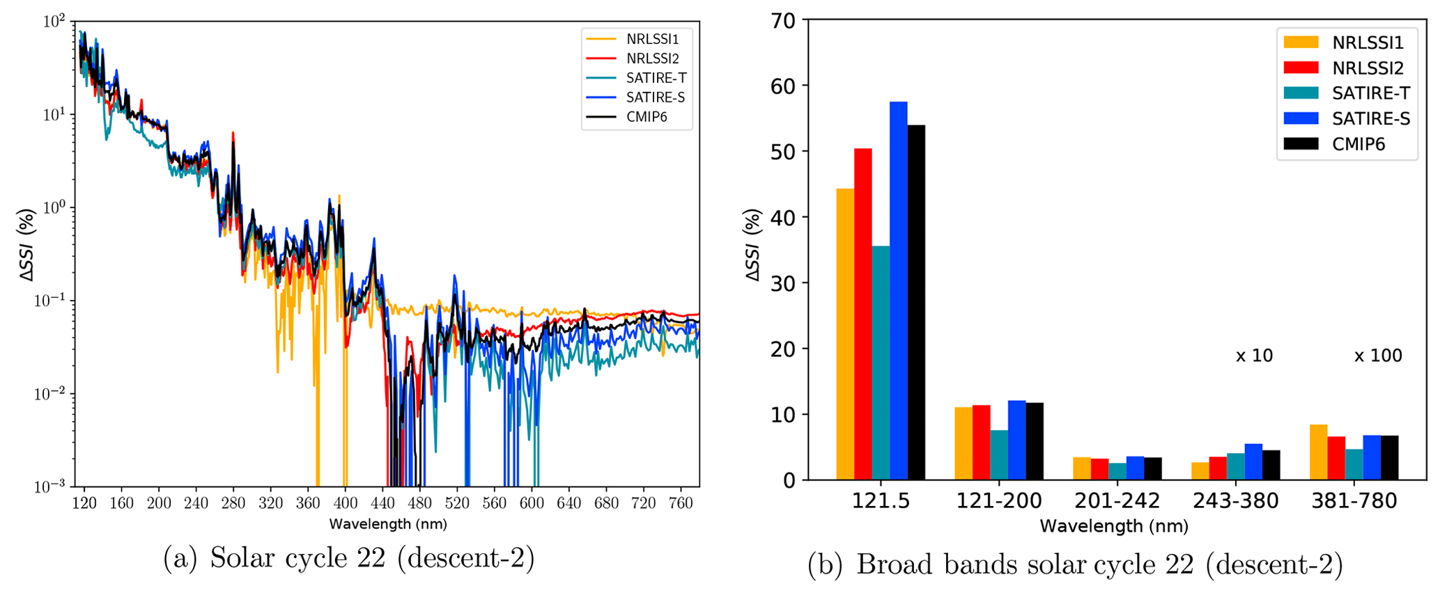
Figure 1(a) Solar cycle SSI variations from November 1989 to November 1994 relative to November 1994 (ΔSSI) in percent for wavelengths ranging from FUV to the visible bands; (b) as in (a) for the Lyman-α (121.5 nm), far-UV (121–200 nm), Herzberg continuum–Hartley bands (201–242 nm), and Hartley and Huggins bands (243–380 nm) (multiplied by a factor of 10) and visible (381–780 nm) (multiplied by a factor of 100).
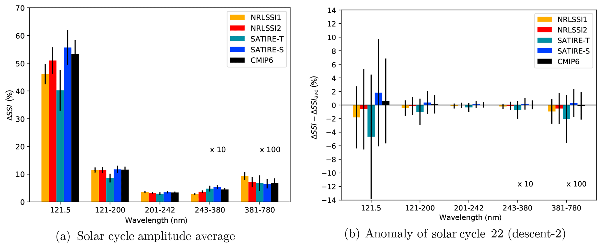
Figure 2(a) Averaged SSI variations for solar cycle amplitudes relative to ATLAS-3 (ΔSSI) in percent for the Lyman-α (121.5 nm), far-UV (121–200 nm), Herzberg continuum and Hartley bands (201–242 nm), Hartley and Huggins bands (243–380 nm) (multiplied by a factor of 10), and visible (381–780 nm) (multiplied by a factor of 100) spectral ranges, with the 95 % confidence interval given as error bar. (b) Anomaly of SSI variations for solar cycle 22 (descent-2) with respect to the averaged solar cycle shown in (a).
2.5 SSI amplitudes
The quantification of the uncertainties of the solar responses in the CCMs is based on an exemplary solar amplitude with decreasing solar irradiances from the maximum of solar cycle 22 in November 1989 to a state near the solar minimum in November 1994, which is motivated by the timing of the ATLAS-3 measurements. Table 1 gives an overview of the applied SSI data sets with details of their percentage solar cycle amplitude in the Lyman-α, far-UV (FUV, 121–200 nm), UV in the Herzberg continuum (partly overlapping with the Hartley bands) (201–242 nm), UV in the Hartley–Huggins bands (243–380 nm), and the visible (381–780 nm) spectral regions. The first value (ΔSSI) represents the percentage SSI change from solar minimum to maximum relative to the ATLAS-3 solar minimum SSI in November 1994 and is also shown in Fig. 1b. The second value represents ΔSSI relative to the TSI change from solar minimum to maximum () in percent. Whereas ΔSSI emphasises the large variability of the solar irradiance at Lyman-α and in the Schumann–Runge continuum and bands over the 11-year solar cycle, the ΔSSI weighted by ΔTSI emphasises the large solar cycle variation in absolute energy in the UV and visible wavelengths. High ΔSSI variability in the FUV is leading to large increases in the photolysis of oxygen and water vapour in the upper mesosphere during solar maximum. More important for the solar response of stratospheric ozone mixing ratios are the two UV spectral regions. While the irradiance increases in the 201–242 nm spectral region lead to more oxygen photolysis and subsequent ozone production in the stratosphere during solar maximum, the irradiance increases between about 243 and 380 nm lead to more ozone destruction through photolysis during solar maximum, further discussed in Sect. 5.1. The NRLSSI1 and NRLSSI2 data sets have the lowest ratio in the Hartley–Huggins UV band among the SSI models used here, whereas the SATIRE-S data set shows the highest and also has the highest ratio in the Lyman-α, FUV, and Herzberg continuum–Hartley band spectral regions.
Table 1Solar cycle spectral solar irradiances changes from November 1989 to November 1994 relative to November 1994 (ΔSSI) in percent and relative contribution of SSI changes to the TSI change () in percent for the Lyman-α (121.5 nm), far-UV (121–200 nm), Herzberg continuum–Hartley bands (201–242 nm), Hartley–Huggins bands (243–380 nm), and visible (381–780 nm) spectral ranges.

The magnitude of the applied solar amplitude in this study can be regarded as representative for the second half of the 21st century when the solar cycles 19 to 23 showed relatively large 11-year solar cycle amplitudes. However, the individual solar cycles show different, spectrally resolved characteristics in their amplitudes, which also differ among the individual SSI data sets. Compared to other solar cycle amplitudes in the satellite era (see Table S1 in the Supplement), the one used in this study is neither especially weak nor especially strong. The averaged ΔSSI is shown in Fig. 2a, with the error bars indicating the 95 % confidence interval of the ΔSSI within each spectral region. The main characteristics of the solar amplitude chosen here are also present in the averaged solar cycle amplitude, such as the small solar amplitude of SATIRE-T in the FUV and most of the ranking of the SSI data sets within the spectral regions. All deviations of the chosen solar cycle amplitude from the averaged solar cycle amplitude are within the range of the 95 % confidence intervals (Fig. 2b). Therefore, the selected solar cycle amplitude can be regarded as representative for most of the solar cycle amplitudes of the satellite era.
Besides the ATLAS-3 reference SSI data set, more recent SSI reference data sets are available such as SOLAR-ISS (Meftah et al., 2020, 2018), which is representative of the 2008 solar minimum. The usage of an alternative SSI reference data set may have an influence on the climatological state of the CCMs, as higher or lower SSI values in certain spectral bands lead to higher or lower SW heating rates, thus affecting the temperature and potentially also the zonal wind of the CCMs. As the reference SSI data set serves as a common base state for the solar minimum of all other SSI data sets, we do not expect significant differences in the uncertainties of the solar responses when using a different SSI reference spectrum.
Two state-of-the-art CCMs have been used in this study to quantify the uncertainty of the modelled solar response related to the 11-year solar cycle. These are EMAC (ECHAM/MESSy Atmospheric Chemistry) (Jöckel et al., 2016) and CESM1(WACCM) (Community Earth System Model 1–Whole Atmosphere Chemistry Climate Model) (Marsh et al., 2013). Both CCMs have a good spectral resolution of their SW radiation and photolysis parameterisation and therefore are well suited for this study. The main difference between EMAC and WACCM, as applied here, is WACCM's model top in the lower thermosphere which allows for a better representation of the chemical processes in the upper mesosphere in WACCM.
3.1 EMAC
EMAC is a CCM that includes sub-models describing tropospheric and middle-atmospheric processes and their interaction with oceans, land, and human influences (Jöckel et al., 2010). It uses the second version of the Modular Earth Sub-model System (MESSy2) to link multi-institutional computer codes. The core atmospheric model is the fifth-generation European Centre Hamburg general circulation model (ECHAM5, Roeckner et al., 2006). For the present study we applied EMAC (ECHAM5 version 5.3.02, MESSy version 2.52; Jöckel et al., 2016) in T42L47MA resolution, i.e. with a spherical truncation of T42 (corresponding to a quadratic Gaussian grid of approx. 2.8∘ latitude by 2.8∘ longitude) with 47 hybrid pressure levels up to 0.01 hPa (∼80 km). EMAC includes the MECCA (Module Efficiently Calculating the Chemistry of the Atmosphere) (R. Sander et al., 2011) chemical mechanism, which contains 155 species with 224 gas-phase, 12 heterogeneous, and 74 photolytic reactions. The photolysis rate coefficients are calculated with JVAL (Sander et al., 2014) using updated rate coefficients recommended by JPL (S. P. Sander et al., 2011) and resolves the solar Lyman-α line and eight spectral bands in the UV and visible ranges (178–683 nm). RAD and RAD-FUBRAD (Dietmüller et al., 2016) provide the parameterisation of radiative transfer based in the SW on Fouquart and Bonnel (1980) and Roeckner et al. (2003) (RAD) with four bands from 250 to 4000 nm. For a better resolution of the UV–vis spectral band RAD-FUBRAD is used for pressures lower than 70 hPa, increasing the spectral resolution in the UV–vis from one band to 55, 81, or 106 bands (Nissen et al., 2007; Kunze et al., 2014). Here we use the updated version of RAD-FUBRAD with 81 bands which substitutes the single-band parameterisation for the heating rates in the Schumann–Runge bands (Strobel, 1978) by the parameterisation based on 19 bands, as given in Strobel (1978), and 14 bands in the Chappuis bands (407.5–690 nm). The stratospheric equatorial zonal winds are relaxed towards an observed Quasi-Biennial Oscillation (QBO) with the sub-model QBO (Giorgetta and Bengtsson, 1999). With an upper boundary in the upper mesosphere, EMAC is not able to capture the thermospheric influx of NOy. Therefore, the simulations presented in this study employ the UBCNOX parameterisation (Sinnhuber et al., 2018; Funke et al., 2016) in the upper mesosphere to include NOy produced in the thermosphere by auroral and medium-energy electrons.
3.2 WACCM
The Whole Atmosphere Community Climate Model (version 4; Marsh et al., 2013) is an integrative part of the Community Earth System Model suite (version 1.0.6; Hurrell et al., 2013). CESM1(WACCM) is a “high-top” CCM covering an altitude range from the surface to the lower thermosphere, i.e. up to hPa, equivalent to approx. 140 km. It is an extension of the Community Atmospheric Model (CAM4; Neale et al., 2013) with all its physical parameterisations. For this study the model has been integrated with a horizontal resolution of 1.9∘ latitude by 2.5∘ longitude and 66 levels in the vertical. CESM1(WACCM) contains a middle-atmosphere chemistry module based on the Model for Ozone and Related Chemical Tracers (MOZART3; Kinnison et al., 2007) which includes a total of 52 species with 127 gas-phase, 17 heterogeneous, and 48 photolytic reactions. A six-constituent ion chemistry model is included with 13 ionisation reactions and 14 ion-neutral and recombination reactions. Its photolysis scheme resolves 100 spectral bands in the UV and visible range (121–750 nm). The SW radiation module is a combination of different parameterisations. Above approx. 70 km the spectral resolution is identical to the photolysis scheme (plus the parameterisation of Solomon and Qian, 2005, based on the F10.7 cm solar radio flux to account for extreme-ultraviolet (EUV) irradiances). Below approx. 60 km the SW radiation of CAM4 is retained, employing 19 spectral bands between 200 and 5000 nm (Collins, 1998). For the transition zone (60–70 km), SW heating rates are calculated as weighted averages of the two approaches. CESM1(WACCM) features relaxation of stratospheric equatorial winds to an observed or idealised (used here) QBO (Matthes et al., 2010). The ionisation in the auroral regions by energetic particles is parameterised according to Roble and Ridley (1987) using the Kp index as an input parameter. To achieve a setup for low auroral activity, for WACCM the Kp index is set to a constant value of Kp =0.67, as this corresponds to a geomagnetic index of Ap =3, which is used in the EMAC sub-model UBCNOX.
3.3 CCM simulations
All EMAC and WACCM simulations have been made explicitly for this study, to ensure that the differences in the solar responses are exclusively related to the SSI data sets prescribed or the CCM applied, and not due to differences in the scenario. For both CCMs (EMAC and WACCM) time slice simulations have been performed with the same basic scenario in all simulations, except only for the prescribed SSI data set. The basic scenario consists of year 2000 conditions for prescribed greenhouse gas (GHG) mixing ratios, ozone-depleting substances (ODSs), and monthly climatological sea surface temperatures (SSTs) and sea ice concentrations (SICs) (average from 1995 to 2004). After dismissing 5 or 3 years of spinup for EMAC and WACCM, respectively, 45 years of data are available from each simulation for analyses. The QBO is included in all simulations by relaxation of the zonal wind in the tropical lower stratosphere between 90 and 10 hPa with the strongest nudging applied from 50 to 15 hPa in EMAC. Whereas EMAC uses the time series of the observed zonal winds (Naujokat, 1986), an idealised 28-month varying QBO is used for WACCM. The reference simulation with perpetual solar minimum conditions, performed by each CCM, uses the ATLAS-3-based SSI reference spectrum (Thuillier et al., 2004; see Sect. 2.1). To our knowledge, this is the first time that this observational SSI data set has been used to force CCM simulations. In addition, five sensitivity simulations with perpetual solar maximum conditions of the solar cycle 22 maximum in November 1989 from five different SSI data sets have been performed by each CCM. The five spectra for solar maximum conditions are constructed by adding the difference of the SSI between the solar maximum in November 1989 and the near solar minimum in November 1994 of NRLSSI1 (Lean, 2000), NRLSSI2 (Coddington et al., 2016), SATIRE-T (Krivova et al., 2010), SATIRE-S (Yeo et al., 2015), and CMIP6-SSI (Matthes et al., 2017) to the common ATLAS-3-based observational reference SSI data set which is defined for the solar minimum state. By this procedure we ensure that we use a common spectral distribution of energy that only varies in the solar maximum sensitivity simulations by the genuine difference from solar minimum to solar maximum of each SSI data set. Table 1 summarises the resulting percentage changes for five spectral regions and also gives an overview of the five sensitivity simulations for solar maximum, which have been performed by WACCM and EMAC.
The solar minimum reference simulation as well as the solar maximum sensitivity simulations are performed for low auroral activity. Due to these model configurations, the NOy changes are expected to be caused by the SSI changes from solar minimum to solar maximum and not by variations in auroral activity.
To analyse the solar response, time series of anomalies have been calculated for each simulation performed by EMAC and WACCM using one of the five SSI data sets constructed for solar maximum conditions with respect to the time series of the reference simulations of both models using the ATLAS-3-based SSI near solar minimum. These five anomaly fields for each CCM can be interpreted as solar response of the model variables to SSI and TSI changes over the 11-year solar cycle. Figure 3 shows the solar response of the ensemble mean, i.e. averaged over the simulations of both CCMs applying five different SSI data sets each, in (a) SW heating rate (HR), (b) temperature, and (c) ozone mixing ratio. The averaged solar response is significant at the 95 % level in regions that are not masked by grey hatching. A t test is applied to the complete concatenated ensemble (10 simulations in each group without performing an ensemble mean of the simulations at solar maximum and minimum in advance). By this procedure the variability of the solar response is maintained and the regions where the significance reaches the 95 % level are smaller compared to the results of a t test for an ensemble average.
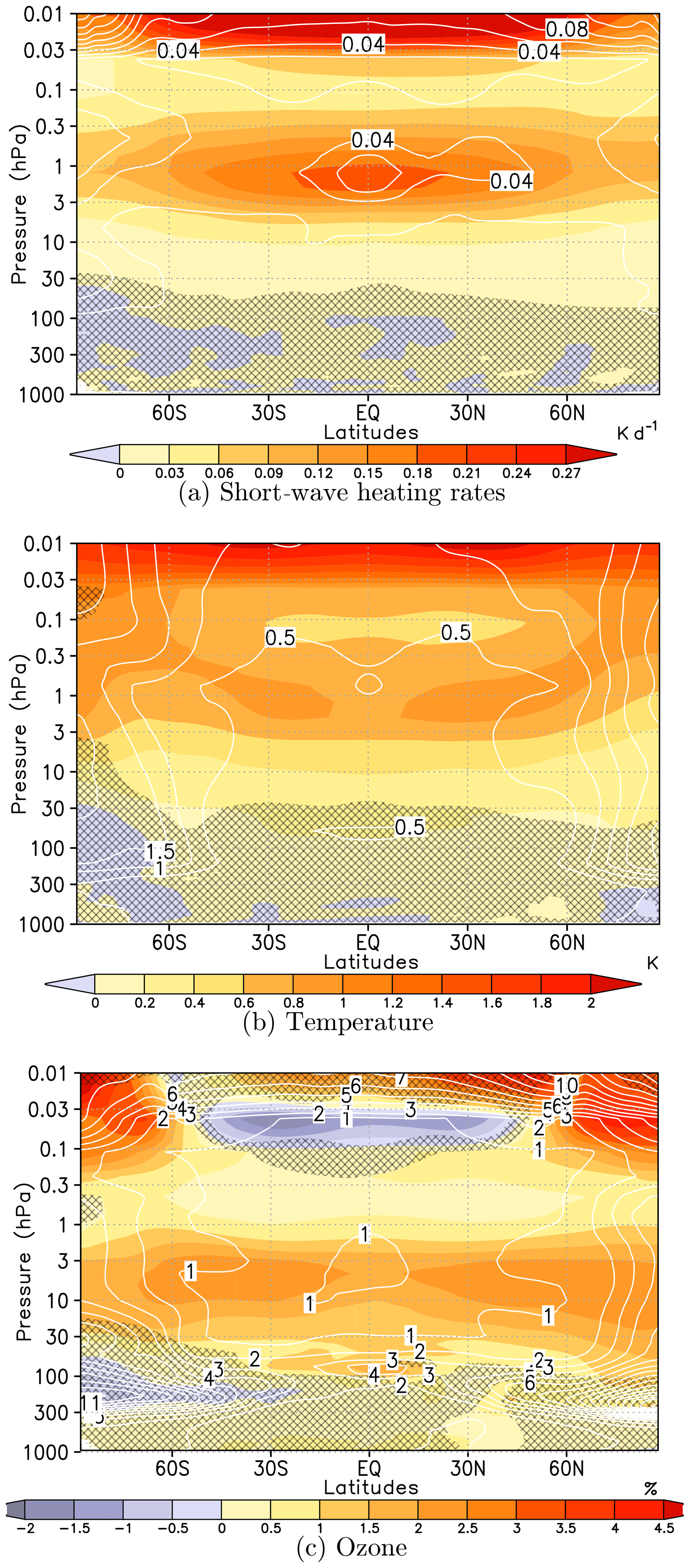
Figure 3Annual mean 11-year solar cycle response (shaded) and signal variance (white contours) in terms of the solar response annual standard deviation for SW heating rates (a), temperature (b), and ozone mixing ratios (c). Solar response derived as ensemble mean over both models and all SSI data sets; solar minimum SSI based on ATLAS-3 reference state. The grey hatching masks areas where signal or ratio of explained variance does not pass a test for statistical significance (p>5 %).
The solar SW heating rate response is significant throughout the middle atmosphere at pressures lower than 30 hPa with peaks in the tropics near the stratopause (∼0.2 K d−1) and in the upper mesosphere (∼0.38 K d−1) (Fig. 3a). Whereas the solar response in the upper mesosphere is due to enhanced solar radiation in the spectral range from Lyman-α to the Schumann–Runge bands (absorbed by oxygen), the solar response near the stratopause is mainly due to an increase over the solar cycle in the Hartley and Huggins bands (absorbed by ozone). The very low standard deviation of the solar response of the ensemble mean throughout the stratosphere and mesosphere (except for the upper-mesospheric polar regions) provides evidence that the primary annual mean radiative response of the middle atmosphere is a robust feature and not particularly sensitive to the specified SSI data set or the CCM configuration.
A direct consequence of the stronger SW heating during solar maximum is a solar response in temperature, which also peaks in the upper mesosphere with up to 2 K and near the stratopause in the subtropics with more than 0.8 K (Fig. 3b). This is weaker than the more than 1 K solar temperature response derived from combined SSU–MSU4 satellite data reported by Randel et al. (2009), but in the same order of magnitude as reported by SPARC CCMVal (2010) for CCMs and slightly larger than analysed by Mitchell et al. (2015) for an ensemble of CMIP5 high-top models. The secondary lower-stratospheric maximum in the solar temperature response in the tropics, which has been identified in reanalyses (e.g. Frame and Gray, 2010), is not present in the ensemble mean. At high latitudes, the solar response in temperature generally shows an enhanced spread between the ensemble members which is due to the high internal dynamical variability of the polar winter atmosphere.
The solar response in ozone mixing ratio has a first peak in the stratosphere near 7 hPa with two regions exceeding 2 %, one in the Southern Hemisphere (SH) extending from mid-latitudes to the subtropics and one in the Northern Hemisphere (NH) extending from the subtropics to polar latitudes. The solar ozone response decreases in the upper stratosphere and lower mesosphere, turns to negative values of up to −1.5 % in the mesosphere, and turns again to large positive values of more than 4.5 % in the upper mesosphere (Fig. 3c). Previous studies analysing the stratospheric solar ozone response in CCMs have found a comparable magnitude. For example, Hood et al. (2015) found a significant 2 %–3 % ozone response to the solar cycle between 1979 and 2005 at a slightly higher altitude near 3–4 hPa in three out of six CCMs within CMIP5. In the upper mesosphere, the solar ozone signal differs between the two CCMs: the negative response in EMAC appears only in a narrow layer from 0.1 to 0.03 hPa in WACCM, where it strongly increases above, dominating the ensemble mean ozone response (s. Fig. 5c). The negative solar ozone signal in EMAC is due to a strong enhancement of H2O photolysis during solar maximum leading to an increase in HOx and enhanced catalytic ozone depletion. The divergent solar responses in ozone in the upper mesosphere between EMAC and WACCM (Fig. 5c) are further discussed in Sect. 5.1.
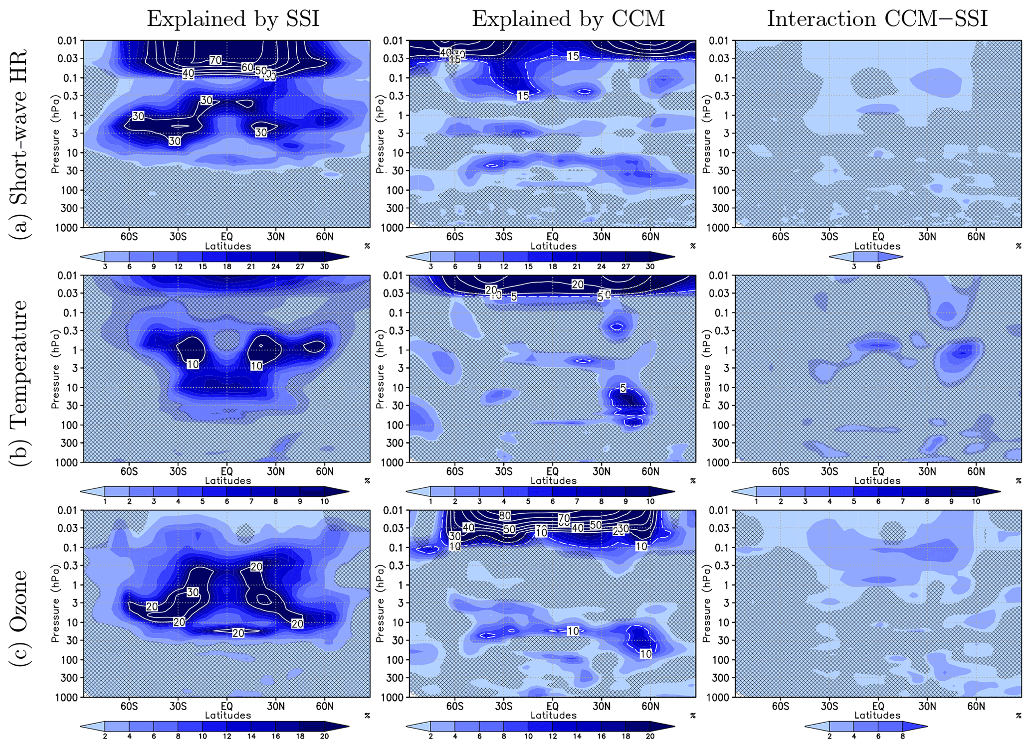
Figure 4Left column: percentage of signal variance (square of white contours of Fig. 3) explained by systematic differences between forcing SSI data sets (Ra,B, Eq. A11, blue shading). The white contours indicate levels of explained variance larger than the range of shading. Middle column: as the left column but for systematic differences between CCMs (Ra,A, Eq. A11). Right column: as the left column but for signal variance explained by the interaction of the CCM and the SSI data set treatments (Ra,AB, Eq. A12). The grey hatching masks areas where the ratio of explained variance does not pass a test for statistical significance (p>5 %).
The averaged solar response discussed in Sect. 4 is supposed to be different with respect to the SSI data set prescribed and with respect to the CCM applied in each run. From the differences in the SSI amplitudes in the broad bands (ΔSSI in Table 1, Fig. 1b), we expect the solar responses to be slightly different for each SSI data set, as we do for each of the CCMs. To quantify the uncertainty of the mean solar response emerging from the usage of different SSI data sets on the one hand and different CCMs on the other, we apply a two-way analysis of variance (ANOVA) approach in this study (see Appendix A for details). The two-way ANOVA is used, as there are two treatments influencing the annual mean solar responses. As these treatments are not applied independently, the interactions of the CCMs and SSI data sets have to be taken into account.
The data set to analyse consists of the annual mean solar responses from simulations using the five SSI data sets in both CCMs, i.e. a time series with 450 years from 10 simulations with 45 years each, as shown for the ensemble average in Fig. 3. The overall variance of the solar response, as expressed by its annual standard deviation (Fig. 3, white contours), is partitioned according to Eq. (A3) into a contribution arising from the applied SSI data sets (SSb,B), a contribution arising from the applied CCMs (SSb,A), the interaction of both treatments (SSb,AB), and an error term (SSw), describing the random, unexplained interannual variances. The results of the ANOVA for the solar response are shown in Fig. 4. The adjusted coefficients of determination Ra,B (left column), Ra,A (middle column), and Ra,AB (right column) (Eqs. A11, A12) are coloured, and additional white contours are included when the values reach or exceed the limits of the colour coding. They indicate the percentage of the solar response variance that can be explained by the differences between the SSI data sets, the CCMs, or the interaction of both treatments. Superimposed grey hatching masks areas where the solar responses are not significantly different when grouped according to the SSI data sets or the CCMs. Note that the contributions of the variances explained by the SSI data set, the CCM, and the interaction of both in Fig. 4 do not add up to 100 %, as often the random contribution to the total variance is largest.
Significant differences in the solar response can be identified when the simulations of the ensemble mean are grouped according to the SSI data sets (Fig. 4, left) and the CCMs (Fig. 4, middle). In the upper mesosphere, differences between the CCMs explain more than 80 % of the spread in the solar ozone signal – due to the change of sign in the ozone response between WACCM and EMAC, more than 25 % of the spread of the solar temperature signal, and up to 50 % of the spread of the SW heating rate signal at high latitudes. In contrast, between 60∘ S and 60∘ N up to 70 % of the spread of the solar response in SW heating rates is explained by the different SSI data sets, due to large solar amplitude variations in the FUV between the SSI data sets. As a result, the SSI data sets also induce a significant fraction of the variability of the solar response in temperature (9 %) at the mesopause.
In the upper stratosphere and lower mesosphere, the SSI data sets are responsible for a relatively large part of the variance of the solar responses, while the CCMs explain much less variance as the radiation schemes of both models possess a sufficient spectral resolution to capture the SW heating rate peak. The largest fractions of the SSI-induced variance of the solar response in SW heating rates (30 %) and ozone (30 %) peak in the subtropics, while the SSI-induced variance of the temperature solar response (10 %) maximises in the tropics.
Compared to Ra,A and Ra,B, the fraction of explained variance by the interaction of the SSI data set and CCM (Ra,AB) is only small. Some significant differences of the solar responses in SW heating rates and ozone are explained by the interaction in the upper mesosphere and near the stratopause for temperature.
In the lower stratosphere and troposphere, the SSI data sets do not contribute significantly to the variability of the solar response in annual mean SW heating rates, temperature, and ozone. But some significant contributions of the applied CCMs to the variance of the solar response are found, which have similar vertical and latitudinal structures for all three variables, peaking in the tropics between 30 and 10 hPa and in the northern subtropics to mid-latitudes between 100 and 10 hPa. The minor CCM contribution to the SW heating rate solar response in the lower stratosphere (p>10 hPa) is consistent with the CCM-induced variance contribution of ozone and seems to be related to differences in ozone transport affecting SW ozone absorption.
The simulations performed with the SATIRE-T data set show considerable deviations in the solar response compared to simulations using the other data sets, as further discussed in Sect. 5.1. When omitting the simulations with the SATIRE-T data set in the ANOVA (see Fig. S1 in the Supplement), less variability is explained by the SSI data set, revealing that a large fraction of the variability attributed to the SSI data set is caused by the specific behaviour of SATIRE-T.
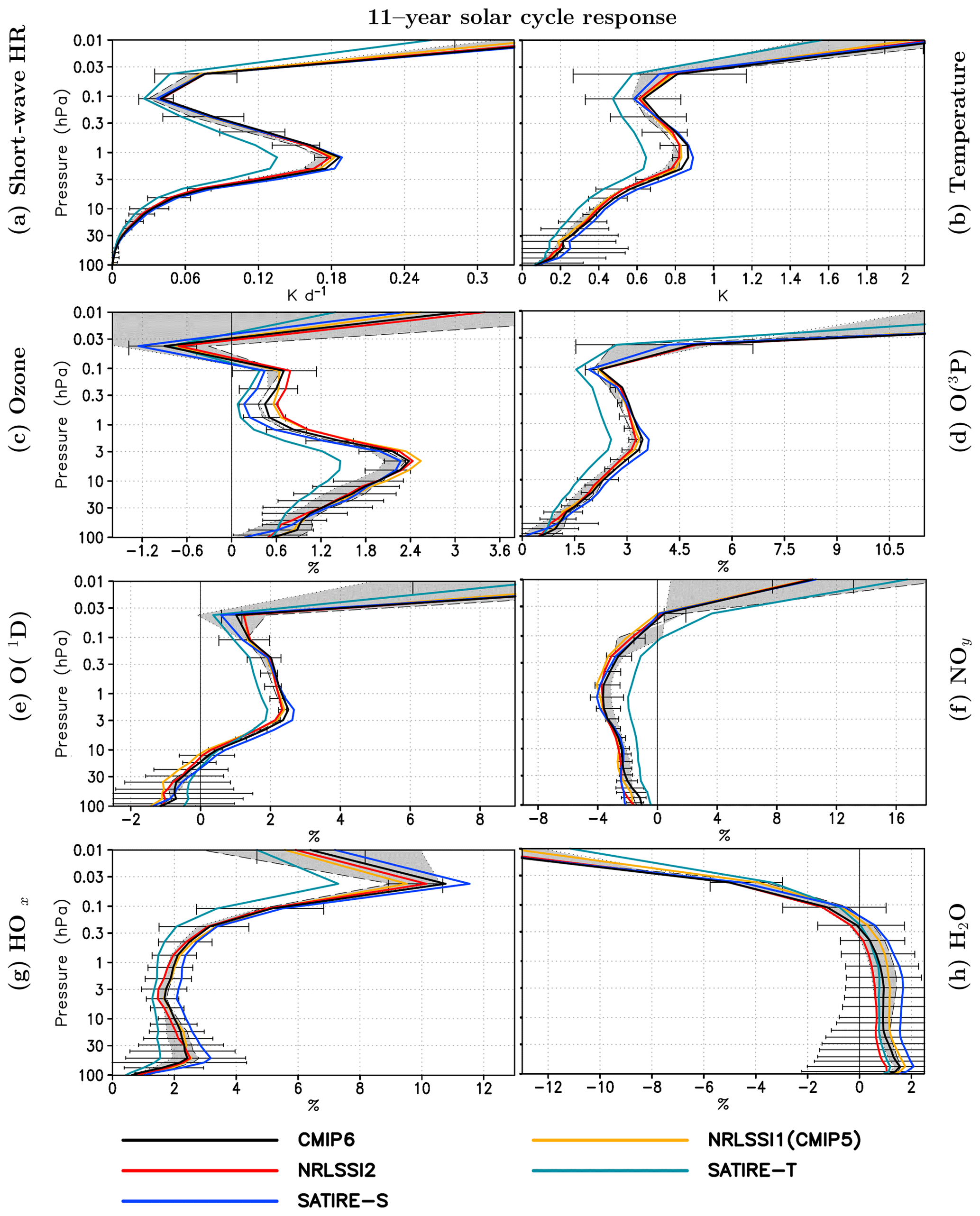
Figure 5Annual mean 11-year solar cycle response (60∘ S–60∘ N) in (a) SW heating rates, (b) temperature, (c) ozone concentrations, (d) atomic oxygen (O(3P)), (e) atomic oxygen (O(1D)), (f) NOy, (g) HOx, and (h) H2O. Solar responses are derived for an average of WACCM and EMAC simulations using five SSI data sets at solar maximum, NRLSSI1(CMIP5) (yellow), NRLSSI2 (red), SATIRE-S (blue), SATIRE-T (dark blue), and CMIP6 (black), relative to the average of the WACCM and EMAC reference solar minimum simulations. The shaded area indicates the range of the WACCM (black long dash contour) and EMAC (black dotted contour) ensemble means. The 95 % uncertainty error bar is given for the averaged solar response over the complete ensemble, calculated with Student's t test.
5.1 Differences resolved by SSI data set
The ANOVA of the ensemble mean in the previous section has shown that significant differences in the solar responses can be attributed to the SSI data sets mainly in the region of the most active ozone production in the upper stratosphere to lower mesosphere, whereas significant differences attributed to the CCMs are mainly located in the upper mesosphere and lower stratosphere, further discussed in Sect. 5.2. In this section, we examine the differences in the solar responses of EMAC and WACCM arising from the use of the different SSI data sets. The atmospheric response to solar irradiance variations is primarily determined by radiative and photochemical processes that are represented by a variety of parameterisations in climate models or CCMs. To separate the effects of differences in the input SSI data sets on the respective SW radiation and photolysis schemes of EMAC and WACCM, we first present profiles for simulations applying the five individual SSI data sets, averaged over both CCMs. Figure 5 shows vertical profiles of the solar cycle amplitude in SW heating rates, temperature, ozone, atomic oxygen (O(3P) and O(1D)), NOy, HOx, and water vapour (H2O), averaged from 60∘ S to 60∘ N between 100 hPa close to the tropopause and 0.01 hPa in the upper mesosphere. For each sub-figure, the 11-year solar response is at first calculated as the difference between the individual solar maximum simulations and the ATLAS-3 solar minimum reference simulation for EMAC and WACCM, respectively. The differences are then grouped according to the SSI data set and averaged over EMAC and WACCM. As in Fig. 3, a t test is applied to the solar response of the complete ensemble. The 95 % confidence interval from this test is included as error bars in each panel of Fig. 5. To better assess the solar responses of the photochemically influenced quantities shown in Fig. 5, the solar responses of the photolysis rates of EMAC and WACCM (averaged over both CCMs as for Fig. 5) are shown in Fig. 6 for a single simulation time step in January at 180∘ E, averaged from 60∘ S to 60∘ N. The shaded areas in Figs. 5 and 6 indicate the range of the solar responses between the EMAC and WACCM ensemble means, framed by the dotted and dashed black contours for the EMAC and WACCM ensemble means, respectively. By comparing the CCM averaged profiles for individual SSI data sets with the SSI averaged ensemble mean for each CCM (shading), the relative roles of the SSI data sets and the CCMs can directly be inferred for the different quantities and altitude regions.
The average over both CCMs shows the strongest stratospheric solar response in SW heating rates and temperatures when using the SATIRE-S data set, whereas SATIRE-T leads to the weakest solar response throughout the middle atmosphere (Fig. 5a, b). In the upper mesosphere, these differences are a direct consequence of the magnitude of the FUV amplitude over the solar cycle (see Table 1) with SATIRE-S showing the largest and SATIRE-T showing the smallest solar response in FUV heating by oxygen absorption/photolysis and subsequent temperature increase. In the stratosphere, the photochemical Chapman cycle is more effective during solar maximum, as shown with the positive solar responses of atomic oxygen (O(1D), O(3P), Fig. 5d, e) and the photolysis rates of oxygen and ozone (JO2, JO3→O(1D), JO3→O(3P), Fig. 6a, c, d). This results in a positive solar response in ozone, peaking in the upper stratosphere near 7 hPa (Fig. 5c). The SATIRE-T solar response in ozone is the weakest in this comparison, as its SSI amplitude in the FUV and 201–242 nm spectral ranges, important for the photochemical ozone production, is considerably weaker (7.6 % and 2.6 %) than in the other SSI data sets (11.1 %–12.1 % and 3.3 %–3.6 %) (Table 1), whereas its SSI amplitude in the ozone-destroying UV band (243–380 nm) is comparable to the other SSI data sets. The two competing, wavelength-dependent effects of ozone production and ozone loss in the Chapman cycle lead to the relative weak solar ozone response in simulations using the SATIRE-T data set. Compared to the SATIRE-T-based simulations, the simulations using the remaining SSI data sets show solar responses in SW heating rates, temperature, and ozone that are relatively close to each other.

Figure 6Percentage change of the photolysis rates from solar minimum to maximum of (a) oxygen (JO2), (b) ozone (JO3 = ), (c) O3-producing O(1D) (JO3→O(1D)), (d) O3-producing O(3P) (JO3→O(3P)), (e) water vapour (JH2O), and (f) nitric oxide (JNO) for a single time step at 180∘ E averaged from 60∘ S to 60∘ N. Changes are derived for an average of WACCM and EMAC simulations using five SSI data sets at solar maximum NRLSSI1(CMIP5) (yellow), NRLSSI2 (red), SATIRE-S (blue), SATIRE-T (dark blue), and CMIP6 (black) relative to the average of the WACCM and EMAC reference solar minimum simulations. The shaded area indicates the range of the WACCM (long black dashed contour) and EMAC (black dotted contour) ensemble means.
Besides the oxygen chemistry of the Chapman cycle, ozone-depleting catalytic cycles, e.g. the HOx and NOx cycles, are involved in contributing to the solar response in ozone. Whereas the HOx catalytic cycle is the most important one in the upper mesosphere, the NOx catalytic cycle dominates in the middle and upper stratosphere. NOy is specified as NOy , but in the mesosphere NOy is very close to the active nitrogen defined as . For all SSI-based averages, the solar response of NOy is negative in the stratosphere and lower mesosphere but positive in the uppermost mesosphere above 0.03 hPa (Fig. 5f). The stratospheric and lower-mesospheric decrease is consistent with Hood and Soukharev (2006), who attributed the negative solar response of NOy in the stratosphere at low latitudes to enhanced photolysis of nitric oxide (NO) by solar FUV irradiance during solar maximum. The major source of NO is the oxidation of nitrous oxide () in the middle stratosphere at low latitudes where the abundance of O(1D) is sufficiently high due to the photolysis of ozone at wavelengths <310 nm (e.g. Seinfeld and Pandis, 2006). The major sinks of NO are photolysis (NO +hν (183 nm nm) → N + O) and the subsequent reaction of NO with atomic nitrogen () in the upper stratosphere, mesosphere, and lower thermosphere (e.g. Minschwaner and Siskind, 1993). During solar maximum, O(1D) increases (Fig. 5e), implying enhanced NO production from N2O. However, at the same time a clear increase in the NO photolysis rates by 8 % to 9 % is found in the stratosphere and mesosphere at solar maximum (Fig. 6f). This increase is the result of the larger solar irradiance amplitude in the FUV in all applied SSI data sets (see Table 1). With enhanced photolysis at solar maximum, the NOy abundances decrease (Fig. 5f). The NOy solar response is of the same magnitude up to the lower mesosphere for all SSI data sets, except for SATIRE-T, which due to its weaker FUV solar amplitude produces a weaker increase in the NO photolysis rates and a weaker negative NOy solar response. The negative NOy solar response results in a slowdown of the catalytic NOx cycle of ozone destruction, which indirectly enhances the positive solar response in ozone (Sukhodolov et al., 2016).
There are two possible reasons for the increase in NOy in the uppermost mesosphere above 0.03 hPa during solar maximum compared to solar minimum. EUV photoionisation of neutrals increases during solar maximum, leading to an increase in electron, ion, and excited species production and subsequently NO above about 80 km. On the other hand, the response of NOy in the uppermost mesosphere could also reflect changes in the auroral NO production in the lower thermosphere. NO in the lower thermosphere is mainly produced by the reaction of an excited nitrogen atom with molecular oxygen () (Marsh et al., 2004). As low auroral activity is prescribed for both the solar minimum reference and the solar maximum simulations, no solar response of thermospheric NO is expected from this reaction. However, NO in the lower thermosphere is also formed by the reaction of the ground state of N with molecular oxygen (). This reaction is strongly temperature dependent and thus more effective in the warmer lower thermosphere during the solar maximum (e.g. Sinnhuber and Funke, 2020).
The solar response in HOx (defined as OH+HO2) (Fig. 5g) is positive throughout the middle atmosphere in all CCM-averaged SSI simulations. In the stratosphere, HOx is mainly produced by reactions of O(1D) with H2O,CH4, or H2 (e.g. ). Increasing abundance of O(1D) (Fig. 5e) during solar maximum conditions is leading to a positive solar response in HOx mixing ratios (Fig. 5g). A clear dependence of the O(1D) and HOx solar responses on the UV-SSI amplitude is found with the largest solar response in the simulations using the SATIRE-S SSI data set. This SSI amplitude dependence of the HOx solar response continues in the upper mesosphere where it is mainly produced by photolysis of water vapour at wavelengths in the Schumann–Runge bands and Lyman-α.
Despite the loss of H2O through reaction with the more abundant O(1D) during solar maximum, the H2O mixing ratios increase during solar maximum in the stratosphere, which is most pronounced when the SATIRE-S SSI data set is used (Fig. 5h). While this signal is not statistically significant for the complete CCM ensemble, there is a significant solar response in the stratosphere for the individual simulations of WACCM. This positive solar response of H2O in the upper stratosphere and lower mesosphere has also been identified in HALOE satellite data by Remsberg et al. (2018). It is explained by chemical reaction of CH4 and H2 with OH, finally producing, after a reaction chain including photolytic reactions, H2O (Remsberg et al., 1984). The positive solar response of H2O in the lower stratosphere corresponds to the positive solar response of temperature in the tropical tropopause layer (TTL) region, which increases the saturation vapour pressure during solar maximum and thus counteracts the water-vapour-limiting freeze-drying mechanism. This is in contrast to the results of Schieferdecker et al. (2015), who analysed water vapour from MIPAS and HALOE satellite instruments and found an anti-correlation of a slightly time-shifted 11-year solar cycle proxy with lower-stratospheric water vapour. In the upper mesosphere, the solar response in H2O is negative as a direct consequence of the stronger water vapour photolysis during solar maximum (Fig. 5h).
In summary, the analysis of CCM-averaged quantities has revealed a dependence of the solar responses on the SSI data sets, with solar responses for most quantities showing a clear relation to the SSI amplitude. Whereas the solar responses are relatively close to each other in the stratosphere and lower mesosphere when using NRLSSI1, NRLSSI2, and CMIP6, clear differences appear for SATIRE-T, which shows the smallest solar responses for all analysed variables. SATIRE-S produces an enhanced solar response for HOx and H2O but agrees well with NRLSSI1, NRLSSI2, and CMIP6 for the other variables. The differences in the SSI amplitude are responsible for 10 % of the temperature, 30 % of the ozone, and up to 40 % of the SW heating rate variability of the solar response in the stratosphere and lower mesosphere. An even larger part of the variability of the solar response in the stratosphere can be attributed to the SSI data set for O(3P) (60 %) and O(1D) (70 %) (see Fig. S3 in the Supplement). In the upper mesosphere, the choice of the SSI data set has the largest influence on the solar response variability of the SW heating rates (70 %) for which the solar amplitude of the SSI data set in the FUV is the main driver.

Figure 7Annual mean temperature deviation of EMAC and WACCM to ERA-5 climatology. (a) EMAC – ERA-5 and (b) WACCM – ERA-5 climatology. The ensemble mean for each CCM consists of the solar minimum reference simulation (included five times in the ensemble mean) and the five simulations of the solar maximum. The ERA-5 data consist of annual mean data from 1982 to 2018. Grey hatching masks areas where differences do not pass a test for statistical significance (p>5 %), for differences relative to ERA-5.
5.2 Differences resolved by CCM
Large differences in the variability of the solar response explained by CCM differences have been identified by the ANOVA (Fig. 3) in the upper mesosphere. The range of the solar responses between the EMAC and WACCM ensemble means over the SSI data sets, indicated by the shaded areas in Figs. 5 and 6, also identifies the largest differences in the upper mesosphere.
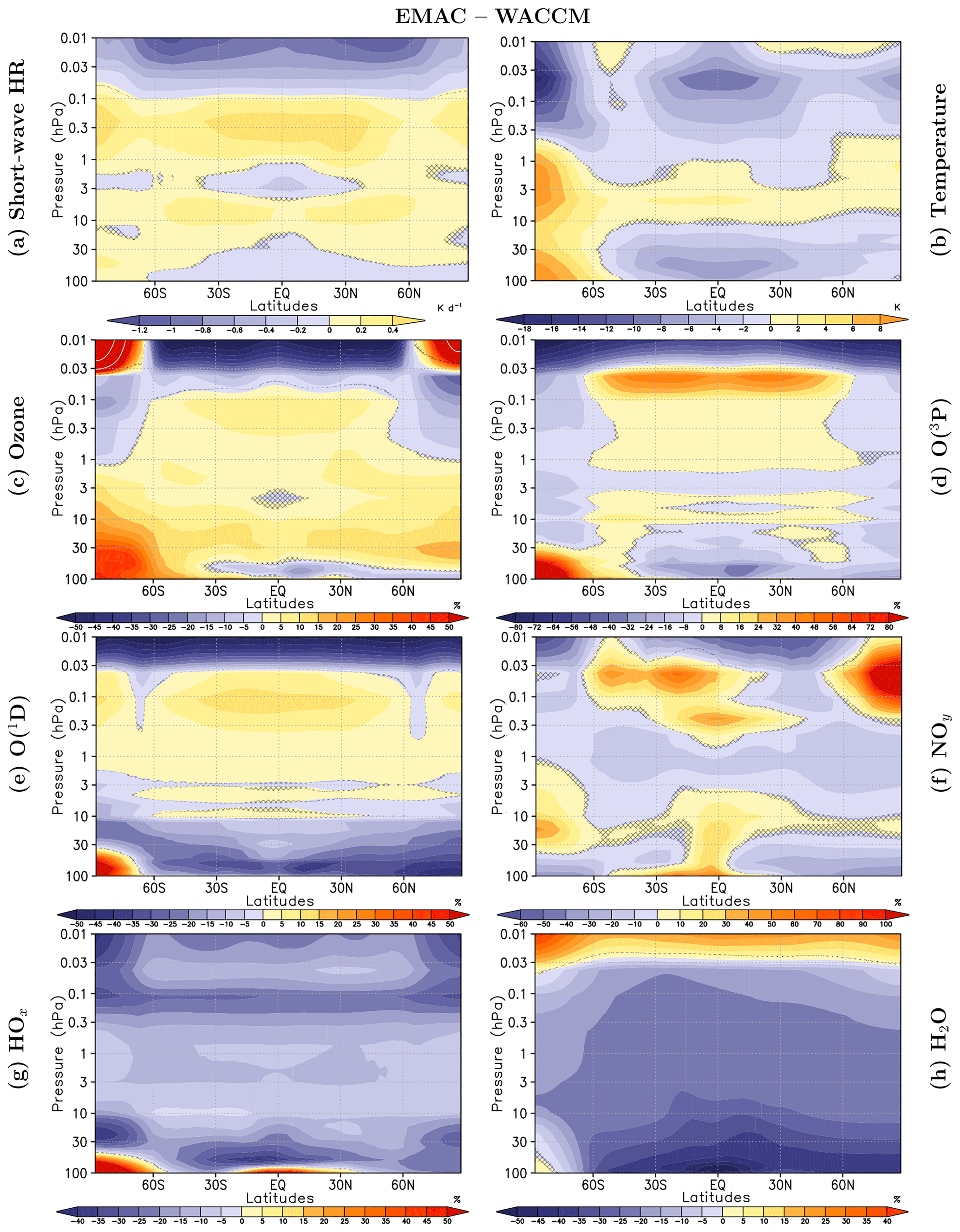
Figure 8Annual mean differences for EMAC (ensemble mean) minus WACCM (ensemble mean) (shaded) of (a) SW heating rates, (b) temperature, (c) ozone mixing ratios, (d) atomic oxygen (O(3P)), (e) HOx, and (f) NOy. The ensemble mean for both CCMs consists of the solar minimum reference simulation (included five times in the ensemble mean) and the five simulations for the solar maximum. Grey hatching masks areas where differences do not pass a test for statistical significance (p>5 %).
The changes in the chemistry and dynamics over the 11-year solar cycle are superimposed on the climatological reference states of the CCMs and are influenced by the climatological temperatures and abundances of photochemically active species. In particular the climatological temperature has a large effect on the chemistry in the middle atmosphere and lower thermosphere either directly on the chemical gas-phase reaction rates or indirectly, as the temperature in the tropical lower stratosphere determines the abundance of H2O in the middle atmosphere and thereby also affects many chemical reactions. The climatological background state of a CCM is determined by a number of factors, ranging from the horizontal and vertical resolutions and the vertical model domain to the physical and chemical processes either resolved or parameterised by the models. In this section, we examine the uncertainty in the atmospheric solar response arising from the model specifications of the EMAC and WACCM models, regarded here as representatives for typical state-of-the-art CCMs. For this purpose, two ensembles of five simulations each for EMAC and WACCM have been constructed by averaging the simulations with different SSI data sets of each model to the respective model ensemble. To achieve an overall ensemble mean representative for a mean solar state, the reference solar minimum simulation in each model ensemble is weighted by a factor of 5, to balance the five simulations with the SSI data sets at solar maximum in each model ensemble.
Figure 7 shows the deviations of the climatological annual mean temperature of EMAC and WACCM from the climatological temperatures of the ERA-5 reanalysis (Hersbach et al., 2018). The ERA-5 climatology includes 37 years from 1982 to 2018 centred around the year 2000. The temperature deviations of both CCMs relative to ERA-5 are largely statistically significant on the 95 % level (all regions not masked by hatching), as estimated by Student's t test.
EMAC has a pronounced cold bias in the tropical upper troposphere–lower stratosphere (UTLS), where WACCM simulates slightly higher temperatures than the ERA-5 climatology. In the upper stratosphere and upper mesosphere, both models show a cold bias over large regions, which is more pronounced in the mesosphere of EMAC. In the lower mesosphere both CCMs show higher temperatures compared to ERA-5. At SH high latitudes, temperatures in WACCM are too low in the stratosphere and too high in the mesosphere compared to the ERA-5 climatology (Fig. 7).
Figure 8 presents a direct comparison between the annual mean climatologies of the EMAC and WACCM ensemble means in the middle atmosphere in terms of zonal mean differences in SW heating rates, temperature, ozone, atomic oxygen (O(3P), O(1D)), NOy, HOx, and H2O. Substantially lower (by up to 1.2 K d−1) SW heating rates are found in the upper mesosphere of EMAC. This bias is indicative of less effective FUV heating from oxygen absorption in the Schumann–Runge bands, presumably due to differences in the O2 absorption parameterisation of Strobel (1978) with 19 bands (used in EMAC) and the heating rates from the photolysis parameterisation based on Koppers and Murtagh (1996) (used in WACCM). These differences in SW parameterisations between the CCMs also affect the solar response in the upper mesosphere which is smaller in EMAC for the SW heating rates and temperatures (Fig. 5a, b). They lead to the patterns of solar response variance explained by CCMs in Fig. 3a, b which resemble the structure of the anomaly pattern in SW heating rates in the upper mesosphere (Fig. 8a). By contrast, in the lower mesosphere and large areas of the stratosphere, EMAC shows higher SW heating rates, possibly an effect of the degraded spectral resolution of the SW radiation scheme in WACCM below 60 km or of the higher ozone mixing ratios in EMAC (Fig. 8c). However, WACCM shows larger solar responses in ozone mixing ratios and JO3→O(3P) photolysis rates in the lower and middle stratosphere, possibly related to the finer spectral resolution of the photolysis scheme used in WACCM.
The temperature deviations in the mesosphere between EMAC and WACCM (Fig. 8b) are not congruent with those in SW heating rates and, therefore, most likely have to be attributed to differences in dynamical heating by dissipating planetary or gravity waves. The largest temperature differences between EMAC and WACCM are located in high southern latitudes. The southern polar vortex is much colder in WACCM than in EMAC and the ERA-5 reanalyses. This shows that with the implementation of the modified gravity wave parameterisation of Garcia et al. (2017) in our WACCM simulations, the low-temperature bias has been alleviated but still exists. Interaction between dynamics and chemistry in EMAC is leading to higher ozone mixing ratios in the lower stratosphere over the south pole, where a less intense and warm-biased south polar vortex is avoiding more severe heterogeneous ozone depletion, compared to WACCM.
Besides the differences in the average mesospheric SW heating rates and temperatures between EMAC and WACCM, there are also large differences in the chemical composition (and the associated solar responses) in this region. The odd oxygen mixing ratios in the upper mesosphere are lower in EMAC by 50 % for ozone, 80 % for O(3P), and more than 50 % for O(1D) (Fig. 8c–e). This is partly explained by the fact that oxygen photolysis in the Schumann–Runge continuum (O2 +hν (λ<175.9 nm) → O(1D)+O(3P)) is neglected in EMAC, because it becomes important only in the lower thermosphere, which is above the upper lid of EMAC. The larger abundances of O(1D) and O(3P) in WACCM, which has a higher upper lid than EMAC, are the result of photochemical production in the lower thermosphere and downward transport into the mesosphere by the residual circulation during the winter seasons, where they affect the climatological averages as well as the solar responses of atomic oxygen, O3, and HOx. The model differences in January and July exhibit a clear enhancement of O(1D) and O(3P) in the respective winter hemisphere of WACCM indicative of strong downward transport from the lower thermosphere (see Figs. S4 and S5 in the Supplement). As a result of the larger O(1D) and O(3P) mixing ratios, the equilibrium of ozone-producing and ozone-destroying processes leads to higher ozone mixing ratios in WACCM, apparent in the climatology (Fig. 8c) as well as in the solar response (Fig. 5c) in the upper mesosphere. Due to the larger solar responses in the mixing ratios of O(1D) and O(3P) (Fig. 5d, e), WACCM produces a strong ozone increase from solar minimum to maximum, in contrast to EMAC, where the more intense HOx cycle at solar maximum (Fig. 5g) dominates and leads to a negative solar response. Noticeable are the higher ozone mixing ratios in the upper-mesospheric high latitudes of EMAC (Fig. 8c) compared to WACCM which result from a less effective catalytic HOx cycle of ozone destruction during the winter seasons, due to much lower HOx mixing ratios in EMAC in these regions.
As already discussed for atomic oxygen in the previous paragraph, the climatologies and solar responses of chemical species in the upper mesosphere are strongly affected by differences in the vertical transport between WACCM and EMAC. With an upper boundary in the lower thermosphere, WACCM is capable to simulate the downward transport of NOy by the gravity-wave-driven residual circulation from the thermosphere down to the lower mesosphere at high latitudes in the respective winter seasons (Figs. S4 and S5 in the Supplement). In EMAC we use the UBCNOX parameterisation to include NOy produced in the thermosphere by auroral and medium-energy electrons. Nevertheless, the NOy mixing ratios are up to 60 % lower in EMAC than in WACCM in large parts of the upper mesosphere, except for northern polar latitudes where the WACCM NOy mixing ratios are exceeded by 100 % (Fig. 5f). The solar response of NOy in the upper mesosphere discussed in Sect. 5.1 is much stronger in WACCM than in EMAC, as obvious from the shaded area in Fig. 2f. In WACCM, the increased NO production during solar maximum in the uppermost mesosphere and lower thermosphere is driven by the increase in EUV photoionisation and lower-thermospheric temperatures as discussed in Sect. 5.1. In EMAC, the NOy mixing ratios in the uppermost four model levels are determined by the UBCNOX parameterisation, which depends on the prescribed, constantly low Ap index but not on the solar UV and EUV radiation and thus suppresses a solar response in NOy.
Differences between EMAC and WACCM are also found in the climatological distribution of water vapour and the related HOx mixing ratio. In the annual mean, EMAC has less H2O than WACCM in the stratosphere and lower mesosphere – except for the upper mesosphere, where EMAC exceeds the WACCM values (Fig. 8h). The lower H2O abundance of EMAC in the middle atmosphere is the consequence of a cold bias in the tropical UTLS region (Fig. 8b), a feature of EMAC also discussed in Jöckel et al. (2016). As a result, HOx, which is produced by photolysis of H2O, is also lower in EMAC (Fig. 8g). From solar minimum to solar maximum, the abundances of H2O (Fig. 5h) and the photolysis rates of H2O (Fig. 6e) increase in the stratosphere and lower mesosphere, leading to a HOx increase by about 2 %–3 % in both models (see also Sect. 5.1). The smaller solar response of HOx in EMAC in this height region can be attributed to differences in the model climatologies because of the lower HOx and H2O mixing ratios in EMAC. In the mesosphere, the magnitude of the solar responses of H2O (negative) and HOx (positive) grow fast with altitude. At solar maximum, strongly enhanced H2O photolysis (Fig. 6e) induces a decrease in H2O (Fig. 5h) and an increase in HOx by about 11 % (Fig. 5g). The HOx production in the upper mesosphere is dominated by H2O photolysis at wavelengths in the Schumann–Runge bands and Lyman-α with the major reaction H2O+hν ( H+OH (70 %, ) and two minor reactions, producing O+2H (12 %, ) and H2+O(1D) (10 %, ) (Nicolet, 1984). However, while the solar responses in H2O photolysis (positive) and H2O mixing ratio (negative) further increase towards the upper mesosphere, the positive solar response in HOx peaks near 70 km and declines above, implying the existence of a HOx-depleting process that increases with solar activity in the upper mesosphere and counteracts HOx production by H2O photolysis. In addition H2O declines in the upper mesosphere, limiting the potential for HOx production. The CCMs start to deviate more strongly in the upper mesosphere, with EMAC showing a less intense decrease in the solar response in HOx than WACCM. This cannot be attributed to the H2O photolysis as EMAC has a larger solar response in H2O photolysis. The reason might be the combination of the up to 50 % larger upper-mesospheric H2O mixing ratio in EMAC (Fig. 8h) and the stronger solar response of WACCM in O(3P) (Fig. 5d) which acts in WACCM as a more effective sink of HOx through reaction . The smaller H2O mixing ratio of WACCM in the upper mesosphere is a consequence of the larger O(1D) mixing ratios in WACCM, leading to a more effective decomposition of water vapour through . During solar maximum this H2O decomposition is even enhanced, due to more abundant O(1D) mixing ratios in the upper mesosphere (Fig. 5e), leading to a more pronounced negative H2O solar response in WACCM (Fig. 5h).
In summary, both models show for all quantities comparable solar responses to the different SSI data sets up to the lower mesosphere near 0.1 hPa. Above, the solar responses deviate substantially, as shown for ozone, oxygen, HOx, and NOy. The comparison of the upper-mesospheric solar responses in EMAC and WACCM, as well as the differences in the climatologies in the upper mesosphere, shows that a realistic simulation of solar cycle effects might be better achieved when the residual downward transport of thermospheric photolysis reactants is taken into account.
In this section we focus on the solar response in total column ozone (TCO) in our simulations and investigate to what extent TCO is influenced by the applied SSI data set and CCM. The solar response in TCO is the vertically integrated solar response in ozone mixing ratios. In the previous sections, we have identified differences in the solar response in ozone mixing ratios depending on the applied SSI data set (Sect. 5.1) as well as on the applied CCM (Sect. 5.2), especially in the middle to lower stratosphere which contributes most to the solar response in TCO.
Hood (1997), who analysed SBUV (solar backscatter ultraviolet) radiometer data for a relatively short period from 1979 to 1993, found an annual mean solar response of TCO in the tropics of 1 %–2 %. For the same time period, Zerefos et al. (1997) detected a significant correlation of the solar activity with annual mean TCO from TOMS between 40∘ S and 40∘ N, whereas no significant correlation was found at higher latitudes, due to the large dynamically induced variability. Soukharev and Hood (2006) suggested that the solar response of TCO is mainly caused by ozone abundances in the tropical lower stratosphere. A study of Randel and Wu (2007) identified a significant annual mean solar response in TCO between 40∘ S and 60∘ N in TOMS and SBUV data from 1979 to 2005.
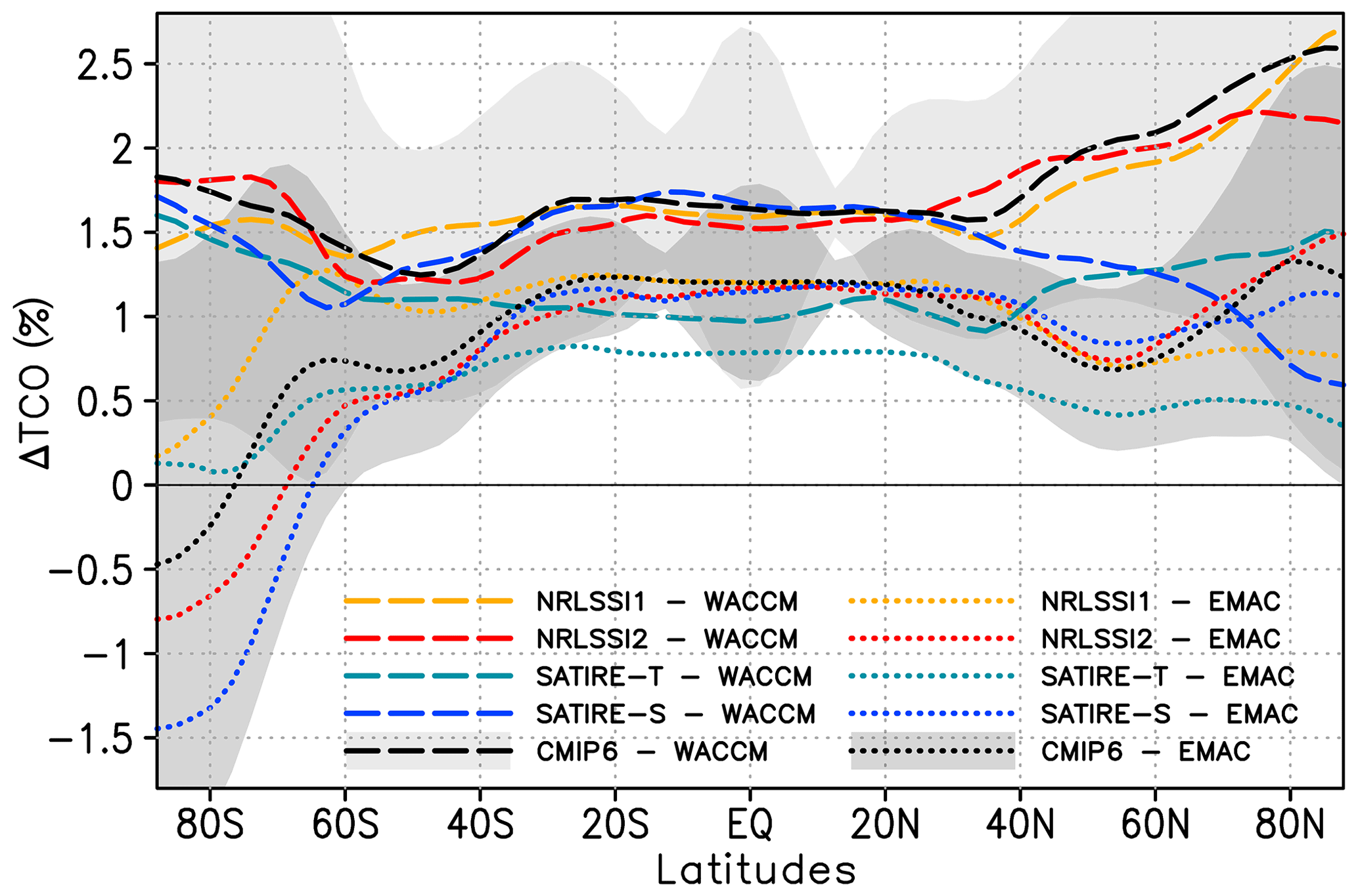
Figure 9Annual mean zonally averaged 11-year solar cycle response in total column ozone (TCO) in percent for WACCM (long dashed) and EMAC (dotted) for prescribed SSI data sets NRLSSI1(CMIP5) (yellow), NRLSSI2 (red), SATIRE-S (blue), SATIRE-T (light blue), and CMIP6 (black). The 95 % uncertainty range is given for simulations with the CMIP6 data set for WACCM (light grey shaded) and EMAC (dark grey shaded).
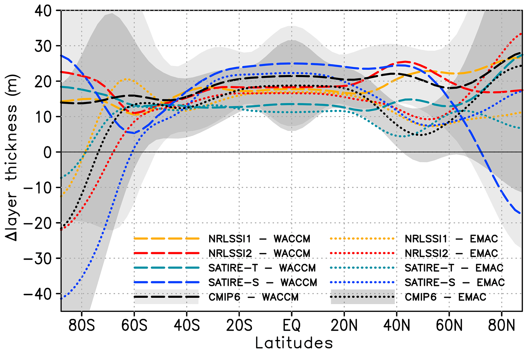
Figure 10Annual mean zonally averaged 11-year solar cycle response in layer thickness from 100 to 10 hPa in metres for WACCM (long dashed) and EMAC (dotted) with prescribed SSI data sets NRLSSI1(CMIP5) (yellow), NRLSSI2 (red), SATIRE-S (blue), SATIRE-T (light blue), and CMIP6 (black). The 95 % uncertainty range is given for simulations with the CMIP6 data set for WACCM (light grey shaded) and EMAC (dark grey shaded).
The latitudinal distribution of the solar response in TCO for the 10 simulations performed for this study is shown in Fig. 9. Clear differences occur between both CCMs, with WACCM showing in general a larger solar response in TCO at all latitudes. Between 40∘ S and 40∘ N significant solar TCO responses are simulated in both models, reaching 1.5 % (3.9 DU) for WACCM and 1.1 % (3.0 DU) for EMAC in the tropics (20∘ S–20∘ N). The chosen SSI data set has only a very minor impact on the solar TCO signal in both models, except for SATIRE-T. The WACCM and EMAC simulations using SATIRE-T show the smallest solar responses in the tropics, which reflects the small solar amplitude in the UV spectral region of this SSI data set. At mid-latitudes and high latitudes, differences in the solar TCO signals between the SSI data sets become larger; however they remain generally smaller than the differences between the models, as is particularly evident for high southern latitudes.
The solar response in TCO at high latitudes is strongly influenced by stratospheric dynamic variability during the respective winter seasons in both hemispheres. As a measure of this dynamic variability, we introduce in Fig. 10 the thickness of the stratospheric layer between the 100 and 10 hPa pressure levels. High values of the 100–10 hPa layer thickness correspond to a warm layer and a weak polar vortex occurring in dynamically disturbed periods, such as minor or major sudden stratospheric warmings (SSWs). The associated downward transport of air in high latitudes leads to an increase in TCO. On the other hand, cold conditions in polar regions, represented by low values of 100–10 hPa layer thickness, can lead to enhanced chemical ozone depletion and low TCO values (Farman et al., 1985; Rex et al., 2002; Manney et al., 2011). While the 100–10 hPa layer thicknesses for all 10 simulations show comparable and significantly increased values at solar maximum between 40∘ S and 40∘ N – consistent with the warming in Fig. 2b, systematic differences occur between the two models at southern high latitudes where EMAC simulates a colder and stronger polar vortex during solar maximum and WACCM shows a warmer and weaker polar vortex (Fig. 10). At northern polar latitudes, both models simulate warmer and weaker polar vortices at solar maximum – except for the SATIRE-S WACCM simulation.
The high correlation between the solar responses in TCO and 100–10 hPa layer thickness at high latitudes is reflected in Table 2, which gives the correlation coefficients between the solar maximum anomalies of the annual average 100–10 hPa layer thickness in the polar region (70–90∘) and the respective TCO anomalies for both hemispheres. The annual mean correlation at high latitudes is mainly a result of the high correlation during the winter–spring seasons of both hemispheres, with the highest correlation occurring in January–February–March (JFM) for the NH and in September–October–November (SON) for the SH (for seasonal correlation coefficients see Table S3 in the Supplement). More intense downwelling of ozone during episodes of stratospheric warming events, or less intense downwelling during cold conditions in combination with a more effective chemical ozone depletion, is the main driver of the TCO anomalies in high latitudes in both hemispheres. Although all anomalies shown in Figs. 9 and 10 are derived for simulations during solar maximum conditions with respect to the simulation during solar minimum conditions, a consistent, significant solar response for TCO and lower-stratospheric layer thickness in polar latitudes can not be found, implying that the derived changes at high latitudes are rather due to random internal dynamical variability in the models than to the external solar forcing.
Table 2Correlations of annual average polar region (70–90∘ N) anomalies (solar maximum – solar minimum) of total column ozone (TCO) and the layer thickness from 100 to 10 hPa. TCO change in DU per 100 m geopotential height change and the 95 % confidence interval.
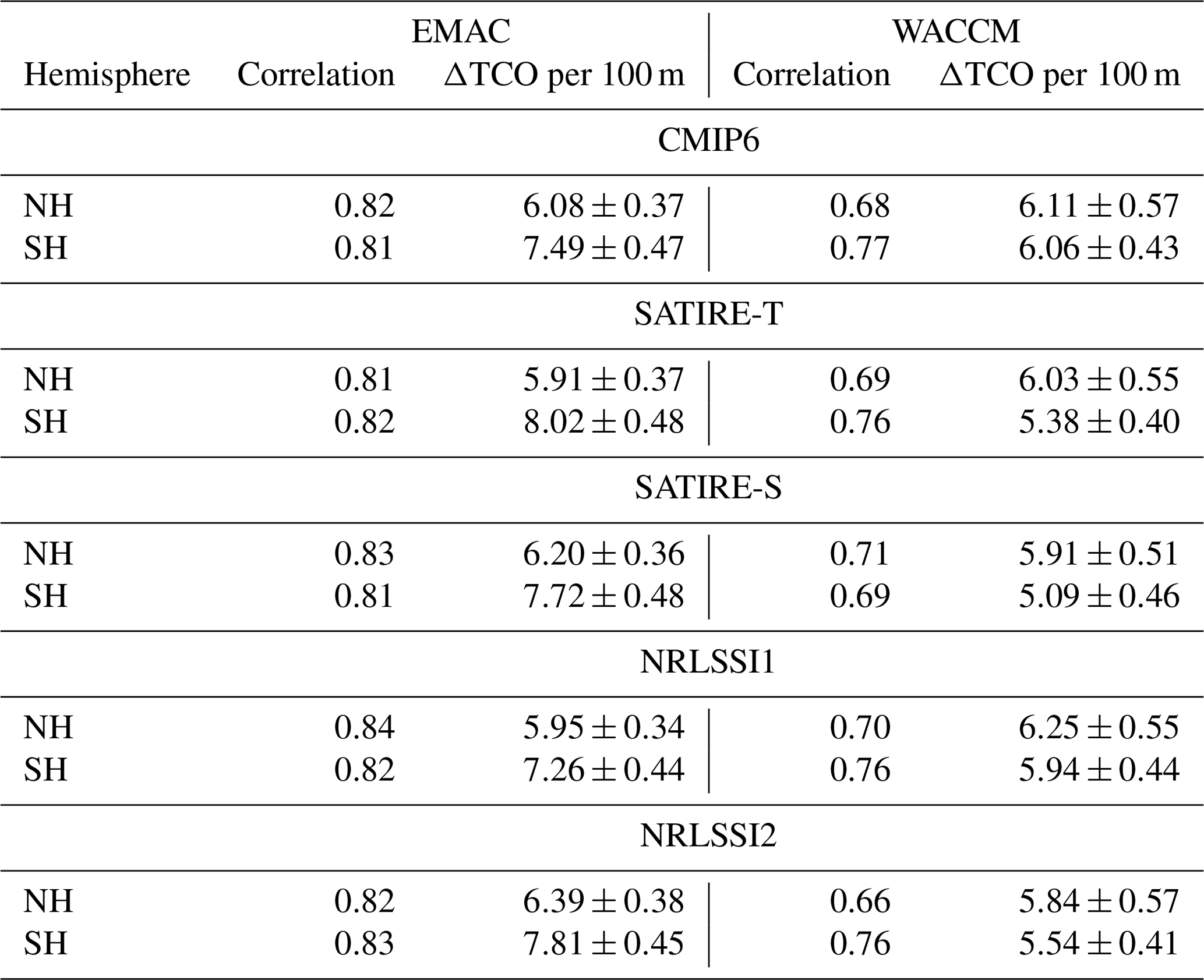
In Fig. 11a we show the zonally averaged differences in TCO between the simulations for solar maximum and solar minimum conditions for the average of all simulations (black contour), the EMAC (blue contour) and WACCM simulations (red contour), the standard deviation (light grey shading), and the two-way ANOVA with SSI (dark grey shading) and CCM treatment (hatches). The range of the standard deviation shows the largest variability of the TCO anomaly in polar regions. As discussed above, the high-latitude TCO anomaly is mainly a result of the internal, dynamic variability of the CCMs. Consequently in the north polar region, there is only a relatively small part of the TCO anomaly variability that can be explained by the SSI data set (1 %) or the CCM (0.6 %). Only in the southern polar region can a larger but still only small fraction of the variability be explained by differences in the CCMs (1.4 %), as there are systematic differences in the anomalies of the lower-stratospheric layer thickness and TCO between WACCM and EMAC (Figs. 9, 10). As in the northern polar region, the SSI data set can only explain a small fraction of the variability of the TCO anomaly in the southern polar region (0.8 %). The standard deviation of the solar TCO response is considerably smaller in the tropics, where the fraction of the standard deviation that can be explained by either the choice of the SSI data set (22 %) or the CCM (13 %) is also much larger, with a larger contribution of the SSI data sets. When approaching the northern mid-latitudes the influence of the CCMs on the variability of the solar response grows, whereas the influence of the SSI data set gets smaller. This is reflected by the pronounced minimum of the solar TCO response in the mid-latitudes of the EMAC simulations, whereas three out of five WACCM simulations show a relatively large positive anomaly in this region.
The annual, global mean solar response of partial column ozone integrated for different pressure regions is shown in Fig. 11b with the same type of contour lines and shading as in Fig. 11a. Averaged over all simulations, the largest solar response in ozone is in the lower stratosphere. In this region, simulations performed by WACCM show a much larger solar response than the averaged EMAC simulations, with the largest differences occurring in the lowest region with pressures higher than 32 hPa. In the WACCM simulations, this layer contributes 32.5 % to the solar response in TCO, whereas it is only 16.7 % in the EMAC simulations. The analysis of SBUV and SBUV/2 data by Hood (1997) shows that 85 % of the solar response in TCO is from the contribution of the lower-stratospheric layer (pressure >16 hPa). The same analysis for the CCMs gives smaller contributions from the lower stratosphere with 52.8 % on average, 57.8 % for WACCM, and 45.3 % for EMAC. This different behaviour of the CCMs in the lower stratosphere is also reflected in the relatively large fraction of the standard deviation of the solar response that can be explained by differences between the CCMs. A larger part of the standard deviation can be explained by differences between the SSI data sets in the middle stratosphere (16–4 hPa), although still the largest part of the standard deviation can not be attributed to either differences between the CCMs or the SSI data sets.
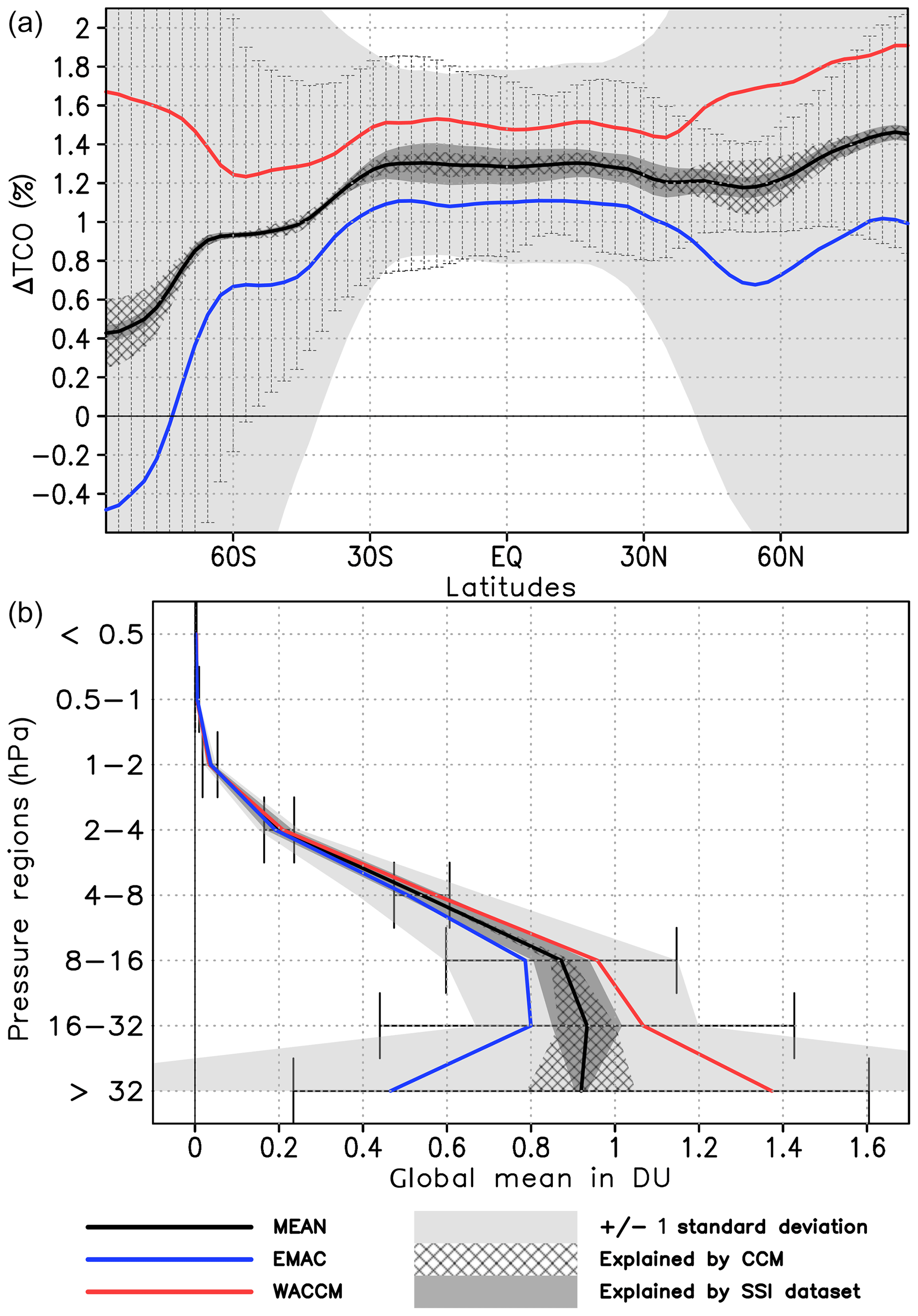
Figure 11(a) Ensemble average, annual, and zonal mean 11-year solar cycle response in partial column ozone in percent (solid black) and the 95 % confidence interval as error bars; WACCM simulations only (solid red); EMAC simulations only (solid blue); light grey shading denotes the standard deviation of the ensemble mean solar response; the hatched region denotes the part of the standard deviation explained by the models; dark shading denotes the part of the standard deviation explained by the SSI data sets. (b) As the top but for annual, global mean 11-year solar cycle response in TCO in DU (solid black) for pressure regions as indicated on the y axis.
This study aimed at investigating the uncertainty in simulations of the atmospheric solar response to 11-year solar cycle variability. In particular, the effects of two sources for uncertainty, i.e. the prescribed spectral solar irradiance (SSI) data set and potential differences in the CCM background state and configuration, were examined. For this purpose, simulations with two CCMs, each forced with five different SSI data sets, were performed. The CCMs EMAC and WACCM are representative of state-of-the-art CCMs, including the prerequisites for simulating solar cycle variability, i.e. spectrally resolved SW radiation and photolysis schemes. Both models contributed to the evaluation of the simulated solar signature in the SPARC CCMVal-2 initiative (SPARC CCMVal, 2010). The SSI data sets represent the best available estimates of 11-year solar variability in electromagnetic radiation and either have been used in previous model studies (i.e. CMIP5 or CCMVal-2) or are recommended for current model intercomparisons (i.e. CMIP6). We apply a novel approach to extract the effects of the pure SSI solar cycle amplitudes, as a common reference SSI distribution for solar minimum conditions was defined, based on ATLAS-3 measurements in November 1994, and SSI data sets for solar maximum were constructed by adding the solar amplitude of the five SSI data sets to the solar minimum reference distribution. To separate the influences of the SSI data sets and the CCMs on the solar responses in SW heating rates, temperature, and ozone, a two-way analysis of variance (ANOVA) was applied here for the first time in this context.
Our study revealed that differences in SSI data sets provide the largest fraction of solar cycle variance in the upper stratosphere–lower mesosphere, contributing 40 % to the SW heating rate, 30 % to the ozone, and 10 % to the temperature solar cycle variance. A second region with a considerable SSI-induced spread in the SW heating rate solar response up to 70 % is the upper mesosphere (except for polar latitudes), also affecting the ozone solar response in this height region. In the region of the largest ozone mixing ratio, in the stratosphere from 50 to 10 hPa, the SSI data sets do not contribute much to the variability of the solar response when SATIRE-T is omitted. Differences between CCMs have a major effect in the upper mesosphere, where they explain more than 80 % of the ozone, 25 % of the temperature, and 50 % of the SW heating rate variability of the solar responses. CCMs add a minor contribution to the SW heating rate and ozone solar cycle variance in the lower stratosphere. However, in the upper stratosphere–lower mesosphere the largest fraction of solar cycle response variance is random and not related to differences in SSI data sets or the applied CCM.
To isolate the causes for the contributions to the solar response spread, a detailed analysis was performed of the solar response profiles of SW heating rate, temperature, ozone, different chemical compounds, and photolysis rates for the five SSI simulation ensemble means (each including two CCMs) on the one hand and for the two CCM ensemble means (each including five SSI data sets) on the other. The analysis of CCM-averaged quantities, involved in the radiative and photochemical processes, has revealed a dependence of the solar responses on the SSI data sets, with solar responses for most quantities showing a clear relation to the SSI amplitude. Whereas the solar responses are relatively close to each other in the stratosphere and lower mesosphere when using NRLSSI1, NRLSSI2, and CMIP6, distinct differences appear for SATIRE-T, which shows the smallest solar responses for all analysed variables. Weaker solar responses in temperature can be explained by a reduced solar cycle amplitude in the 201–242 nm spectral irradiance range, mainly responsible for solar radiative heating in this height range. The ozone increase at solar maximum in the middle and upper stratosphere is the combined result of enhanced oxygen chemistry in the photochemical Chapman cycle and reduced ozone destruction in the NOy catalytic cycle. The NRLSSI1, NRLSSI2, and CMIP6 data sets produce similar solar responses in O(1D), O(3P), and NOy at solar maximum in the stratosphere. The solar ozone signal is considerably weaker in the SATIRE-T data set, as its SSI amplitude in the FUV and 201–242 nm spectral ranges, important for photochemical ozone production, is considerably weaker than in the other SSI data sets, whereas its SSI amplitude in the ozone-destroying UV band (243–380 nm) is comparable. Positive solar responses were also derived for HOx and H2O throughout the middle atmosphere for all SSI data sets. In the stratosphere, where HOx is mainly produced by reactions of O(1D) with H2O, CH4, or H2, the increasing abundance of O(1D) during solar maximum conditions leads to a positive solar response in HOx mixing ratios. A clear dependence of the O(1D) and HOx solar responses on the UV-SSI amplitude was found with the largest solar response in the simulations using the SATIRE-S SSI data set. The increase in H2O mixing ratios with the solar cycle throughout the stratosphere, emerging for all SSI data sets, can be explained by chemical production in the upper stratosphere and enhanced H2O transport from the troposphere into the lower stratosphere in a warmer UTLS at solar maximum. In the upper mesosphere, the choice of the SSI data set has the largest influence on the solar response variability of the SW heating rates (70 %) for which the solar amplitude of the SSI data set in the FUV is the main driver.
In addition to the SSI-induced spread in the solar response, differences between the CCMs turned out to have their strongest impact on the solar responses in SW heating rates, temperature, and ozone in the upper mesosphere at altitudes above about 60 km. The two CCMs used for this study are representative for the current CCM generation which consists primarily of models with a top level in the upper mesosphere around 0.01 hPa (or 80 km altitude), like the EMAC version used in this study, plus a few CCMs that also include the thermosphere, like WACCM with a top level at about 140 km. Resulting differences in the radiation parameterisations and the vertical transport of substances have been identified to cause the spread in the upper-mesosphere solar responses. For example, the spread in the solar response of the upper-mesosphere SW heating rates arises from an underestimation of oxygen absorption in the FUV by the parameterisation of Strobel (1978) in EMAC, reaching up to −1.2 K d−1 compared to WACCM in the climatological annual mean. Moreover, the odd oxygen mixing ratios in the upper mesosphere are substantially lower in EMAC than in WACCM, as EMAC – due to its lower lid – does not capture the photochemical production of O(1D) and O(3P) in the lower thermosphere of WACCM nor their downward transport into the mesosphere by the residual circulation during the winter seasons. As a result, solar ozone responses of opposite sign are produced in the upper stratosphere where WACCM exhibits more ozone at solar maximum due to its enhanced odd oxygen abundances, while EMAC exhibits less ozone due to its more intense HOx cycle. This shows that a realistic simulation of solar cycle effects is better achieved when the residual downward transport of thermospheric photolysis reactants is taken into account. Some of these effects could be included in CCMs with a model top in the upper mesosphere by a thoroughly formulated upper-boundary condition, as already included for NOy produced in the thermosphere by auroral and medium-energy electrons.
For annual mean total column ozone (TCO) a significant solar response could be identified from the southern mid-latitudes to the northern polar region when all simulations from both CCMs are considered. In the southern high latitudes, these TCO anomalies are the result of natural dynamical variability of the Antarctic polar vortex. Distinct differences in TCO anomalies between the CCMs are also expressed by the relatively large fraction of the anomaly variability that can be explained by differences between the CCMs. The usage of the SSI data set has the largest influence on the variability of the TCO solar response in the tropics. The largest contribution to the annual mean TCO solar response is from the lower-stratospheric layers with pressures >16 hPa, which on average contribute 53 %, or when analysed separately, 58 % (WACCM) and 45 % (EMAC). Both CCMs underestimate the lower-stratospheric contribution to the solar response in TCO, compared to the analysis of SBUV and SBUV/2 data by Hood (1997), who found a 85 % contribution of the lower stratosphere to the TCO solar response.
Note that the individual contributions of the SSI data sets and CCM configurations derived in our study are constrained by the choice of the CCMs. While the possible spread of solar cycle SSI variation is very well captured in our study by considering the five currently usable SSI data sets, a similar coverage of the CCM-induced spread cannot be achieved, given the number and diversity of available CCMs. Thus, the CCM contribution to the variance of the solar response is, to some extent, determined by the specifics of the EMAC and WACCM models. For example, the CCM contribution to the solar SW heating rate signal would increase in models applying SW radiation schemes with low spectral resolution or employing TSI scaling procedures.
The usage of an alternative SSI reference data set such as that of Meftah et al. (2020, 2018), which is representative of the 2008 solar minimum, may have an influence on the climatological state of the CCMs, as higher or lower SSI values in certain spectral bands lead to higher or lower SW heating rates, thus affecting the temperature and potentially also the zonal wind of the CCMs. As the reference SSI data set serves as a common base state for the solar minimum of all other SSI data sets, we do not expect significant differences in the uncertainties of the solar responses when using a different SSI reference spectrum. The quantification of the uncertainties of the solar responses in the CCMs is based on only one exemplary solar amplitude (descending phase of solar cycle 22, November 1989 to November 1994). However, other solar cycles show different, spectrally resolved characteristics in their amplitudes, which also differ among the individual SSI data sets. From comparison to other solar cycle amplitudes we found the magnitude of the applied solar amplitude in this study to be representative for solar cycle amplitudes in the satellite era.
Finally, as all simulations of this study were carried out under conditions of low auroral activity, only effects of 11-year variations in solar electromagnetic radiation have been considered in this study. The impact of variations in energetic particle precipitation for different levels of auroral activity will be subject of further studies.
A two-way analysis of variance (ANOVA) (Fisher, 1925) is applied to the time series of anomaly data xijk, i.e. a data set consisting of the time series of the differences between the simulations performed by both CCMs () for solar maximum conditions of five SSI data sets () and the respective simulation of each CCM for solar minimum conditions. It is created by using the five simulations of each CCM with solar maximum SSI data sets minus the simulations of each CCM with the ATLAS-3 SSI data set at solar minimum. Thus, the complete time series consists of 450 annual mean anomalies (nt) from 10 simulations, each with a length of 45 years (n). The anomalies xijk are the individual solar responses, and their fluctuations around the averaged solar response can be described as
with αi the deviations of the averages of the two CCMs from the overall average ; βj the deviations of the averages of simulations applying the five SSI data sets from ; γij the deviations of the averages of the individual simulations , , and from ; and ϵijk the random fluctuations that cannot be explained by αi, βj, or γij. The null hypotheses (H0) are that the averaged solar response does not depend on the CCM (), the applied SSI data set (), or the interaction of CCM with applied SSI data set (). We apply the two-way ANOVA to test the validity of these hypotheses. The total sum of squares (SSt) of the complete time series is calculated as
with the individual annual mean solar response xijk and the overall mean . The SSt of the complete time series is further split by applying two treatments as
One treatment (A) takes into consideration the applied CCM, building two groups (NA=2), the WACCM and the EMAC solar responses with nA=225 elements each. The second treatment (B) takes into consideration the applied SSI data set, building five groups (NB=5) with nB=90 elements each. For each treatment (K= A, B) the sums of squares between the groups (SSb,K) are calculated as
with , the mean solar response of each group, NA, NB the number of groups within each treatment, and nA, nB the number of elements within each group. The sum of squares emerging by the interaction of the treatments (SSb,AB) is calculated as
with the mean of the individual simulations and , the mean solar responses of each group within the treatments. The sum of squares within (SSw), which accounts for the random, unexplained or error part of the variability, is calculated as
with xijk the individual solar responses. The degrees of freedom of the model are calculated as
These are the degrees of freedom within the groups (dfd), which is the degrees of freedom of the denominators when calculating the F statistics (Eq. A15), dfn,K the degrees of freedom between the groups, and dfn,AB the degrees of freedom of the interaction between the treatments which are the degrees of freedom of the nominators in Eq. (A15). Note that the CMIP6 SSI data set depends on the SATIRE-S and NRLSSI2 data sets and therefore cannot be counted as an independent SSI data set. For the calculations of the degrees of freedom we use NB=4. By the ratios
the adapted coefficients of determination (von Storch and Zwiers, 1999) are calculated, which are a measure of the variance explained by the treatment (K= A, B) or by the interaction between both treatments. , , and are shown in Fig. 4. The mean sum of squares within the groups MSSw is calculated as
and the mean sum of squares between the groups MSSb,K and the MSS interacting between the groups MSSb,AB are calculated as
As MSSw, MSSb,K, and MSSb,AB are assumed to be unbiased estimators of the variance σ2 we can use these estimators to calculate the F statistics as
The data of the EMAC and CESM1(WACCM) simulations, which have been performed for this study, are available for download on request.
The supplement related to this article is available online at: https://doi.org/10.5194/acp-20-6991-2020-supplement.
MK wrote the manuscript and performed the EMAC simulations and the data analyses; TK performed the WACCM simulations and contributed to the manuscript; UL initiated the study, acquired the BMBF funding, and participated in writing the manuscript; KM and MS initiated the study, acquired the BMBF funding, and contributed to the manuscript; TR contributed to the manuscript and the EMAC model development.
The authors declare that they have no competing interests.
This article is part of the special issue “The Modular Earth Submodel System (MESSy) (ACP/GMD inter-journal SI)”. It is not associated with a conference.
This study is supported by the German Ministry of Research (BMBF) within the nationally funded project ROMIC-SOLIC. Markus Kunze acknowledges support by the Deutsche Forschungsgemeinschaft (DFG). The EMAC simulations have been performed on the massive parallel supercomputing system of the North-German Supercomputing Alliance (HLRN). All WACCM simulations have been performed on the high-performance computing facilities of Kiel University (Christian-Albrechts-Universität zu Kiel).
This research has been supported by the BMBF (grant no. 01LG1219) and the DFG (grant no. KU 3632/2-1).
This paper was edited by Franz-Josef Lübken and reviewed by three anonymous referees.
Ball, W. T., Unruh, Y. C., Krivova, N., Solanki, S. K., and Harder, J. W.: Solar irradiance variability : a six-year comparison between SORCE observations and the SATIRE model, Astro. Astrophys., 530, A71, https://doi.org/10.1051/0004-6361/201016189, 2011. a
Ball, W. T., Krivova, N. A., Unruh, Y. C., Haigh, J. D., and Solanki, S. K.: A New SATIRE-S Spectral Solar Irradiance Reconstruction for Solar Cycles 21–23 and Its Implications for Stratospheric Ozone, J. Atmos. Sci., 71, 4086–4101, https://doi.org/10.1175/JAS-D-13-0241.1, 2014. a
Ball, W. T., Haigh, J. D., Rozanov, E. V., Kuchar, A., Sukhodolov, T., Tummon, F., Shapiro, A. V., and Schmutz, W.: High solar cycle spectral variations inconsistent with stratospheric ozone observations, Nat. Geosci., 9, 206–209, https://doi.org/10.1038/ngeo2640, 2016. a
Ball, W. T., Alsing, J., Staehelin, J., Davis, S. M., Froidevaux, L., and Peter, T.: Stratospheric ozone trends for 1985–2018: sensitivity to recent large variability, Atmos. Chem. Phys., 19, 12731–12748, https://doi.org/10.5194/acp-19-12731-2019, 2019. a
Beig, G., Fadnavis, S., Schmidt, H., and Brasseur, G. P.: Inter-comparison of 11-year solar cycle response in mesospheric ozone and temperature obtained by HALOE satellite data and HAMMONIA model, J. Geophys. Res.-Atmos., 117, D00P10, https://doi.org/10.1029/2011JD015697, 2012. a
Coddington, O., Lean, J. L., Pilewskie, P., Snow, M., and Lindholm, D.: A Solar Irradiance Climate Data Record, B. Am. Meteorol. Soc., 97, 1265–1282, https://doi.org/10.1175/BAMS-D-14-00265.1, 2016. a, b, c
Coddington, O., Lean, J., Pilewskie, P., Snow, M., Richard, E., Kopp, G., Lindholm, C., DeLand, M., Marchenko, S., Haberreiter, M., and Baranyi, T.: Solar Irradiance Variability: Comparisons of Models and Measurements, Earth Space Sci., 34, 2019EA000693, https://doi.org/10.1029/2019EA000693, 2019. a
Collins, W. D.: A global signature of enhanced shortwave absorption by clouds, J. Geophys. Res.-Atmos., 103, 31669–31679, https://doi.org/10.1029/1998JD200022, 1998. a
Dietmüller, S., Jöckel, P., Tost, H., Kunze, M., Gellhorn, C., Brinkop, S., Frömming, C., Ponater, M., Steil, B., Lauer, A., and Hendricks, J.: A new radiation infrastructure for the Modular Earth Submodel System (MESSy, based on version 2.51), Geosci. Model Dev., 9, 2209–2222, https://doi.org/10.5194/gmd-9-2209-2016, 2016. a
Ermolli, I., Matthes, K., Dudok de Wit, T., Krivova, N. A., Tourpali, K., Weber, M., Unruh, Y. C., Gray, L., Langematz, U., Pilewskie, P., Rozanov, E., Schmutz, W., Shapiro, A., Solanki, S. K., and Woods, T. N.: Recent variability of the solar spectral irradiance and its impact on climate modelling, Atmos. Chem. Phys., 13, 3945–3977, https://doi.org/10.5194/acp-13-3945-2013, 2013. a, b, c, d
Evin, G., Hingray, B., Blanchet, J., Eckert, N., Morin, S., and Verfaillie, D.: Partitioning Uncertainty Components of an Incomplete Ensemble of Climate Projections Using Data Augmentation, J. Climate, 32, 2423–2440, https://doi.org/10.1175/JCLI-D-18-0606.1, 2019. a
Farman, J. C., Gardiner, B. G., and Shanklin, J. D.: Large losses of total ozone in Antarctica reveal seasonal ClOx/NOx interaction, Nature, 315, 207–210, https://doi.org/10.1038/315207a0, 1985. a
Fisher, R.: Statistical methods for research workers, Edinburgh Oliver & Boyd, 1925. a, b
Forster, P. M., Fomichev, V. I., Rozanov, E., Cagnazzo, C., Jonsson, A. I., Langematz, U., Fomin, B., Iacono, M. J., Mayer, B., Mlawer, E., Myhre, G., Portmann, R. W., Akiyoshi, H., Falaleeva, V., Gillett, N., Karpechko, A., Li, J., Lemennais, P., Morgenstern, O., Oberländer, S., Sigmond, M., and Shibata, K.: Evaluation of radiation scheme performance within chemistry climate models, J. Geophys. Res.-Atmos., 116, D10302, https://doi.org/10.1029/2010JD015361, 2011. a
Fouquart, Y. and Bonnel, B.: Computations of solar heating of the Earth's atmosphere: A new parameterization, Beitr. Phys. Atmos., 53, 35–62, 1980. a
Frame, T. and Gray, L. J.: The 11-yr solar cycle in ERA-40 data: An update to 2008, J. Climate, 23, 2213–2222, https://doi.org/10.1175/2009JCLI3150.1, 2010. a
Funke, B., López-Puertas, M., Stiller, G. P., Versick, S., and von Clarmann, T.: A semi-empirical model for mesospheric and stratospheric NOy produced by energetic particle precipitation, Atmos. Chem. Phys., 16, 8667–8693, https://doi.org/10.5194/acp-16-8667-2016, 2016. a
Garcia, R. R., Solomon, S., Roble, R. G., and Rusch, D. W.: A numerical response of the middle atmosphere to the 11-year solar cycle, Planet. Space Sci., 32, 411–423, https://doi.org/10.1016/0032-0633(84)90121-1, 1984. a, b
Garcia, R. R., Smith, A. K., Kinnison, D. E., de la Cámara, Á., and Murphy, D. J.: Modification of the Gravity Wave Parameterization in the Whole Atmosphere Community Climate Model: Motivation and Results, J. Atmos. Sci., 74, 275–291, https://doi.org/10.1175/JAS-D-16-0104.1, 2017. a
Geinitz, S., Furrer, R., and Sain, S. R.: Bayesian multilevel analysis of variance for relative comparison across sources of global climate model variability, Int. J. Climatol., 35, 433–443, https://doi.org/10.1002/joc.3991, 2015. a
Giorgetta, M. A. and Bengtsson, L.: Potential role of the quasi-biennial oscillation in the stratosphere-troposphere exchange as found in water vapor in general circulation model experiments, J. Geophys. Res.-Atmos., 104, 6003–6019, https://doi.org/10.1029/1998JD200112, 1999. a
Gray, L. J., Beer, J., Geller, M., Haigh, J. D., Lockwood, M., Matthes, K., Cubasch, U., Fleitmann, D., Harrison, G., Hood, L., Luterbacher, J., Meehl, G. A., Shindell, D., van Geel, B., and White, W.: Solar influences on climate, Rev. Geophys., 48, RG4001, https://doi.org/10.1029/2009RG000282, 2010. a
Gray, L. J., Scaife, A. A., Mitchell, D. M., Osprey, S., Ineson, S., Hardiman, S., Butchart, N., Knight, J., Sutton, R., and Kodera, K.: A lagged response to the 11 year solar cycle in observed winter Atlantic/European weather patterns, J. Geophys. Res.-Atmos., 118, 13405–13420, https://doi.org/10.1002/2013JD020062, 2013. a
Haberreiter, M., Schöll, M., Dudok de Wit, T., Kretzschmar, M., Misios, S., Tourpali, K., and Schmutz, W.: A new observational solar irradiance composite, J. Geophys. Res.-Space, 122, 5910–5930, https://doi.org/10.1002/2016JA023492, 2017. a
Haigh, J. D.: The role of stratospheric ozone in modulating the solar radiative forcing of climate, Nature, 370, 544–546, https://doi.org/10.1038/370544a0, 1994. a, b
Haigh, J. D., Winning, A. R., Toumi, R., and Harder, J. W.: An influence of solar spectral variations on radiative forcing of climate, Nature, 467, 696–699, https://doi.org/10.1038/nature09426, 2010. a
Hersbach, H., De Rosnay, P., Bell, B., Schepers, D., Simmons, A., Soci, C., Abdalla, S., Balmaseda, A., Balsamo, G., Bechtold, P., Berrisford, P., Bidlot, J., De Boisséson, E., Bonavita, M., Browne, P., Buizza, R., Dahlgren, P., Dee, D., Dragani, R., Diamantakis, M., Flemming, J., Forbes, R., Geer, A., Haiden, T., Hólm, E., Haimberger, L., Hogan, R., Horányi, A., Janisková, M., Laloyaux, P., Lopez, P., Muñoz-Sabater, J., Peubey, C., Radu, R., Richardson, D., Thépaut, J.-N., Vitart, F., Yang, X., Zsótér, E., and Zuo, H.: Operational global reanalysis: progress, future directions and synergies with NWP including updates on the ERA5 production status, Tech. Rep. 8th October, ECWWF, https://doi.org/10.21957/tkic6g3wm, 2018. a
Hood, L. L.: The solar cycle variation of total ozone: Dynamical forcing in the lower stratosphere, J. Geophys. Res.-Atmos., 102, 1355–1370, https://doi.org/10.1029/96JD00210, 1997. a, b, c
Hood, L. L. and Soukharev, B. E.: Solar induced variations of odd nitrogen: Multiple regression analysis of UARS HALOE data, Geophys. Res. Lett., 33, 101029, https://doi.org/10.1029/2006GL028122, 2006. a
Hood, L. L., Misios, S., Mitchell, D. M., Rozanov, E., Gray, L. J., Tourpali, K., Matthes, K., Schmidt, H., Chiodo, G., Thiéblemont, R., Shindell, D., and Krivolutsky, A.: Solar signals in CMIP-5 simulations: the ozone response, Q. J. Roy. Meteorol. Soc., 141, 2670–2689, https://doi.org/10.1002/qj.2553, 2015. a, b
Hurrell, J. W., Holland, M. M., Gent, P. R., Ghan, S., Kay, J. E., Kushner, P. J., Lamarque, J.-F., Large, W. G., Lawrence, D., Lindsay, K., Lipscomb, W. H., Long, M. C., Mahowald, N., Marsh, D. R., Neale, R. B., Rasch, P., Vavrus, S., Vertenstein, M., Bader, D., Collins, W. D., Hack, J. J., Kiehl, J., and Marshall, S.: The Community Earth System Model: A Framework for Collaborative Research, B. Am. Meteorol. Soc., 94, 1339–1360, https://doi.org/10.1175/BAMS-D-12-00121.1, 2013. a
Jöckel, P., Kerkweg, A., Pozzer, A., Sander, R., Tost, H., Riede, H., Baumgaertner, A., Gromov, S., and Kern, B.: Development cycle 2 of the Modular Earth Submodel System (MESSy2), Geosci. Model Dev., 3, 717–752, https://doi.org/10.5194/gmd-3-717-2010, 2010. a
Jöckel, P., Tost, H., Pozzer, A., Kunze, M., Kirner, O., Brenninkmeijer, C. A. M., Brinkop, S., Cai, D. S., Dyroff, C., Eckstein, J., Frank, F., Garny, H., Gottschaldt, K.-D., Graf, P., Grewe, V., Kerkweg, A., Kern, B., Matthes, S., Mertens, M., Meul, S., Neumaier, M., Nützel, M., Oberländer-Hayn, S., Ruhnke, R., Runde, T., Sander, R., Scharffe, D., and Zahn, A.: Earth System Chemistry integrated Modelling (ESCiMo) with the Modular Earth Submodel System (MESSy) version 2.51, Geosci. Model Dev., 9, 1153–1200, https://doi.org/10.5194/gmd-9-1153-2016, 2016. a, b, c
Kinnison, D. E., Brasseur, G. P., Walters, S., Garcia, R. R., Marsh, D. R., Sassi, F., Harvey, V. L., Randall, C. E., Emmons, L., Lamarque, J. F., Hess, P., Orlando, J. J., Tie, X. X., Randel, W., Pan, L. L., Gettelman, A., Granier, C., Diehl, T., Niemeier, U., and Simmons, A. J.: Sensitivity of chemical tracers to meteorological parameters in the MOZART-3 chemical transport model, J. Geophys. Res.-Atmos., 112, 1–24, https://doi.org/10.1029/2006JD007879, 2007. a
Kodera, K. and Kuroda, Y.: Dynamical response to the solar cycle, J. Geophys. Res., 107, 4749, https://doi.org/10.1029/2002JD002224, 2002. a
Kopp, G. and Lean, J. L.: A new, lower value of total solar irradiance: Evidence and climate significance, Geophys. Res. Lett., 38, L01706, https://doi.org/10.1029/2010GL045777, 2011. a, b
Koppers, G. A. A. and Murtagh, D. P.: Model studies of the influence of O2 photodissociation parameterizations in the Schumann-Runge bands on ozone related photolysis in the upper atmosphere, Ann. Geophys., 14, 68–79, https://doi.org/10.1007/s00585-996-0068-9, 1996. a
Krivova, N. A., Solanki, S. K., Wenzler, T., and Podlipnik, B.: Reconstruction of solar UV irradiance since 1974, J. Geophys. Res., 114, D00I04, https://doi.org/10.1029/2009JD012375, 2009. a, b
Krivova, N. A., Vieira, L. E. A., and Solanki, S. K.: Reconstruction of solar spectral irradiance since the Maunder minimum, J. Geophys. Res.-Space 115, A12112, https://doi.org/10.1029/2010JA015431, 2010. a, b
Kruschke, T., Kunze, M., Matthes, K., Langematz, U., Sinnhuber, M., Reddmann, T., Versick, S., and Funke, B.: Quantifying uncertainties of climate signals related to the 11 year solar cycle – Part II: Dynamical impacts of irradiance and auroral forcing, in preparation, 2020. a
Kunze, M., Godolt, M., Langematz, U., Grenfell, J., Hamann-Reinus, A., and Rauer, H.: Investigating the early Earth faint young Sun problem with a general circulation model, Planet. Space Sci., 98, 77–92, https://doi.org/10.1016/j.pss.2013.09.011, 2014. a
Labitzke, K.: Sunspots, the QBO, and the stratospheric temperature in the north polar region, Geophys. Res. Lett., 14, 535–537, 1987. a
Labitzke, K. and van Loon, H.: Associations between the 11-year solar cycle, the QBO and the atmosphere. Part I: The troposphere and stratosphere in the northern hemisphere winter, J. Atmos. Sol.-Terr. Phys., 50, 197–206, 1988. a
Lean, J., Rottman, G., Kyle, H. L., Woods, T., Hickey, J., and Puga, L.: Detection and parameterization of variations in solar mid- and near-ultraviolet radiation, J. Geophys. Res., 102, 29939–29956, https://doi.org/10.1029/97JD02092, 1997. a
Lean, J. L.: Evolution of the Sun's spectral irradiance since the Maunder Minimum, Geophys. Res. Lett., 27, 2425–2428, https://doi.org/10.1029/2000GL000043, 2000. a, b, c
Lean, J. L., Cook, J., Marquette, W., and Johannesson, A.: Magnetic Sources of the Solar Irradiance Cycle, Astrophys. J., 492, 390–401, https://doi.org/10.1086/305015, 1998. a
Manney, G. L., Santee, M. L., Rex, M., Livesey, N. J., Pitts, M. C., Veefkind, P., Nash, E. R., Wohltmann, I., Lehmann, R., Froidevaux, L., Poole, L. R., Schoeberl, M. R., Haffner, D. P., Davies, J., Dorokhov, V., Gernandt, H., Johnson, B., Kivi, R., Kyrö, E., Larsen, N., Levelt, P. F., Makshtas, A., McElroy, C. T., Nakajima, H., Parrondo, M. C., Tarasick, D. W., von der Gathen, P., Walker, K. A., and Zinoviev, N. S.: Unprecedented Arctic ozone loss in 2011, Nature, 478, 469–475, https://doi.org/10.1038/nature10556, 2011. a
Marsh, D. R., Solomon, S. C., and Reynolds, A. E.: Empirical model of nitric oxide in the lower thermosphere, J. Geophys. Res.-Space, 109, A07301, https://doi.org/10.1029/2003JA010199, 2004. a
Marsh, D. R., Garcia, R. R., Kinnison, D. E., Boville, B. A., Sassi, F., Solomon, S. C., and Matthes, K.: Modeling the whole atmosphere response to solar cycle changes in radiative and geomagnetic forcing, J. Geophys. Res., 112, D23306, https://doi.org/10.1029/2006JD008306, 2007. a
Marsh, D. R., Mills, M. J., Kinnison, D. E., Lamarque, J.-F., Calvo, N., and Polvani, L. M.: Climate Change from 1850 to 2005 Simulated in CESM1(WACCM), J. Climate, 26, 7372–7391, https://doi.org/10.1175/JCLI-D-12-00558.1, 2013. a, b
Matthes, K., Langematz, U., Gray, L. L., Kodera, K., and Labitzke, K.: Improved 11-year solar signal in the Freie Universität Berlin Climate Middle Atmosphere Model (FUB-CMAM), J. Geophys. Res.-Atmos., 109, D06101, https://doi.org/10.1029/2003JD004012, 2004. a
Matthes, K., Marsh, D. R., Garcia, R. R., Kinnison, D. E., Sassi, F., and Walters, S.: Role of the QBO in modulating the influence of the 11 year solar cycle on the atmosphere using constant forcings, J. Geophys. Res.-Atmos., 115, d18110, https://doi.org/10.1029/2009JD013020, 2010. a
Matthes, K., Funke, B., Andersson, M. E., Barnard, L., Beer, J., Charbonneau, P., Clilverd, M. A., Dudok de Wit, T., Haberreiter, M., Hendry, A., Jackman, C. H., Kretzschmar, M., Kruschke, T., Kunze, M., Langematz, U., Marsh, D. R., Maycock, A. C., Misios, S., Rodger, C. J., Scaife, A. A., Seppälä, A., Shangguan, M., Sinnhuber, M., Tourpali, K., Usoskin, I., van de Kamp, M., Verronen, P. T., and Versick, S.: Solar forcing for CMIP6 (v3.2), Geosci. Model Dev., 10, 2247–2302, https://doi.org/10.5194/gmd-10-2247-2017, 2017. a, b, c, d
Maycock, A. C., Matthes, K., Tegtmeier, S., Thiéblemont, R., and Hood, L.: The representation of solar cycle signals in stratospheric ozone – Part 1: A comparison of recently updated satellite observations, Atmos. Chem. Phys., 16, 10021–10043, https://doi.org/10.5194/acp-16-10021-2016, 2016. a
McCormack, J. P. and Hood, L. L.: Apparent solar cycle variations of upper stratospheric ozone and temperature: Latitude and seasonal dependences, J. Geophys. Res.-Atmos., 101, 20933–20944, https://doi.org/10.1029/96JD01817, 1996. a
Meehl, G. A., Arblaster, J. M., Matthes, K., Sassi, F., and van Loon, H.: Amplifying the Pacific Climate System Response to a Small 11-Year Solar Cycle Forcing, Science, 325, 1114–1118, https://doi.org/10.1126/science.1172872, 2009. a
Meftah, M., Damé, L., Bolsée, D., Hauchecorne, A., Pereira, N., Sluse, D., Cessateur, G., Irbah, A., Bureau, J., Weber, M., Bramstedt, K., Hilbig, T., Thiéblemont, R., Marchand, M., Lefèvre, F., Sarkissian, A., and Bekki, S.: SOLAR-ISS: A new reference spectrum based on SOLAR/SOLSPEC observations, Astron. Astrophys., 611, A1, https://doi.org/10.1051/0004-6361/201731316, 2018. a, b
Meftah, M., Damé, L., Bolsée, D., Pereira, N., Snow, M., Weber, M., Bramstedt, K., Hilbig, T., Cessateur, G., Boudjella, M.-Y., Marchand, M., Lefèvre, F., Thiéblemont, R., Sarkissian, A., Hauchecorne, A., Keckhut, P., and Bekki, S.: A New Version of the SOLAR-ISS Spectrum Covering the 165–3000 nm Spectral Region, Solar Phys., 295, 14, https://doi.org/10.1007/s11207-019-1571-y, 2020. a, b
Merkel, A., Harder, J. W., Marsh, D. R., Smith, A. K., Fontenla, J. M., and Woods, T. N.: The impact of solar spectral irradiance variability on middle atmospheric ozone, Geophys. Res. Lett., 38, 1–6, https://doi.org/10.1029/2011GL047561, 2011. a, b
Minschwaner, K. and Siskind, D. E.: A new calculation of nitric oxide photolysis in the stratosphere, mesosphere, and lower thermosphere, J. Geophys. Res.-Atmos., 98, 20401, https://doi.org/10.1029/93JD02007, 1993. a
Misios, S., Mitchell, D. M., Gray, L. J., Tourpali, K., Matthes, K., Hood, L., Schmidt, H., Chiodo, G., Thiéblemont, R., Rozanov, E., and Krivolutsky, A.: Solar signals in CMIP-5 Simulations: Effects of Atmosphere–ocean Coupling, Q. J. Roy. Meteor. Soc., 142, 928–941, https://doi.org/10.1002/qj.2695, 2015. a
Mitchell, D. M., Misios, S., Gray, L. J., Tourpali, K., Matthes, K., Hood, L., Schmidt, H., Chiodo, G., Thiéblemont, R., Rozanov, E., Shindell, D., and Krivolutsky, A.: Solar signals in CMIP-5 simulations: the stratospheric pathway, Q. J. Roy. Meteor. Soc., 141, 2390–2403, https://doi.org/10.1002/qj.2530, 2015. a, b
Naujokat, B.: An update of the observed Quasi-Biennial Oscillation of the stratospheric winds over the tropics, J. Atmos. Sci., 43, 1873–1877, 1986. a
Neale, R. B., Richter, J., Park, S., Lauritzen, P. H., Vavrus, S. J., Rasch, P. J., and Zhang, M.: The Mean Climate of the Community Atmosphere Model (CAM4) in Forced SST and Fully Coupled Experiments, J. Climate, 26, 5150–5168, https://doi.org/10.1175/JCLI-D-12-00236.1, 2013. a
Nissen, K. M., Matthes, K., Langematz, U., and Mayer, B.: Towards a better representation of the solar cycle in general circulation models, Atmos. Chem. Phys., 7, 5391–5400, https://doi.org/10.5194/acp-7-5391-2007, 2007. a, b
Oberländer, S., Langematz, U., Matthes, K., Kunze, M., Kubin, A., Harder, J., Krivova, N. A., Solanki, S. K., Pagaran, J., and Weber, M.: The influence of spectral solar irradiance data on stratospheric heating rates during the 11 year solar cycle, Geophys. Res. Lett., 39, L01801, https://doi.org/10.1029/2011GL049539, 2012. a
Randel, W., Smith, K., Austin, J., Barnett, J., Claud, C., Gillett, N., Keckhut, P., Langematz, U., Lin, R., Long, C., Mearsm, C., Miller, A., Nash, J., Seidel, D., Thompson, D., Wu, F., and Yoden, S.: An update of stratospheric temperature trends, J. Geophys. Res., 114, D02107, https://doi.org/10.1029/2005JD006744, 2009. a
Randel, W. J. and Wu, F.: A stratospheric ozone profile data set for 1979–2005: Variability, trends, and comparisons with column ozone data, J. Geophys. Res., 112, D06313, https://doi.org/10.1029/2006JD007339, 2007. a, b
Remsberg, E., Russell, J. M., Gordley, L. L., Gille, J. C., and Bailey, P. L.: Implications of the Stratospheric Water Vapor Distribution as Determined from the Nimbus 7 LIMS Experiment, J. Atmos. Sci., 41, 2934–2948, https://doi.org/10.1175/1520-0469(1984)041<2934:IOTSWV>2.0.CO;2, 1984. a
Remsberg, E., Damadeo, R., Natarajan, M., and Bhatt, P.: Observed Responses of Mesospheric Water Vapor to Solar Cycle and Dynamical Forcings, J. Geophys. Res.-Atmos., 123, 3830–3843, https://doi.org/10.1002/2017JD028029, 2018. a
Rex, M., Salawitch, R. J., Harris, N. R. P., von der Gathen, P., Braathen, G. O., Schulz, A., Deckelmann, H., Chipperfield, M., Sinnhuber, B.-M., Reimer, E., Alfier, R., Bevilacqua, R., Hoppel, K., Fromm, M., Lumpe, J., Küllmann, H., Kleinböhl, A., Bremer, H., von König, M., Künzi, K., Toohey, D., Vömel, H., Richard, E., Aikin, K., Jost, H., Greenblatt, J. B., Loewenstein, M., Podolske, J. R., Webster, C. R., Flesch, G. J., Scott, D. C., Herman, R. L., Elkins, J. W., Ray, E. A., Moore, F. L., Hurst, D. F., Romashkin, P., Toon, G. C., Sen, B., Margitan, J. J., Wennberg, P., Neuber, R., Allart, M., Bojkov, B. R., Claude, H., Davies, J., Davies, W., De Backer, H., Dier, H., Dorokhov, V., Fast, H., Kondo, Y., Kyrö, E., Litynska, Z., Mikkelsen, I. S., Molyneux, M. J., Moran, E., Nagai, T., Nakane, H., Parrondo, C., Ravegnani, F., Skrivankova, P., Viatte, P., and Yushkov, V.: Chemical depletion of Arctic ozone in winter 1999/2000, J. Geophys. Res., 107, 8276, https://doi.org/10.1029/2001JD000533, 2002. a
Roble, R. G. and Ridley, E. C.: An auroral model for the NCAR thermosphere general circulation model (TGCM), Ann. Geophys., 6, 369–383, 1987. a
Roeckner, E., Bäuml, G., Bonaventura, L., Brokopf, R., Esch, M., Giorgetta, Hagemann, S., Kirchner, I., Kornblueh, L., Manzini, E., Rhodin, A., Schlese, U., Schulzweida, U., and Tompkins, A.: The atmospheric general circulation model ECHAM5, Part I, Tech. Rep. No. 349, Max-Planck-Institut für Meteorologie, Hamburg, 2003. a
Roeckner, E., Brokopf, R., Esch, M., Giorgetta, M., Hagemann, S., Kornblueh, L., Manzini, E., Schlese, U., and Schulzweida, U.: Sensitivity of Simulated Climate to Horizontal and Vertical Resolution in the ECHAM5 Atmosphere Model, J. Climate, 19, 3771–3791, https://doi.org/10.1175/JCLI3824.1, 2006. a
Sander, R., Baumgaertner, A., Gromov, S., Harder, H., Jöckel, P., Kerkweg, A., Kubistin, D., Regelin, E., Riede, H., Sandu, A., Taraborrelli, D., Tost, H., and Xie, Z.-Q.: The atmospheric chemistry box model CAABA/MECCA-3.0, Geosci. Model Dev., 4, 373–380, https://doi.org/10.5194/gmd-4-373-2011, 2011. a
Sander, R., Jöckel, P., Kirner, O., Kunert, A. T., Landgraf, J., and Pozzer, A.: The photolysis module JVAL-14, compatible with the MESSy standard, and the JVal PreProcessor (JVPP), Geosci. Model Dev., 7, 2653–2662, https://doi.org/10.5194/gmd-7-2653-2014, 2014. a
Sander, S. P., Abbatt, J., Barker, J. R., Burkholder, J. B., Friedl, R. R., Golden, D. M., Huie, R. E., Kolb, C. E., Kurylo, M. J., Moortgat, G. K., Orkin, V. L., and Wine, P. H.: Chemical Kinetics and Photochemical Data for Use in Atmospheric Studies, Tech. Rep. Evaluation No. 17, JPL Publication 10-6, Jet Propulsion Laboratory, Pasadena, 2011. a
Schieferdecker, T., Lossow, S., Stiller, G. P., and von Clarmann, T.: Is there a solar signal in lower stratospheric water vapour?, Atmos. Chem. Phys., 15, 9851–9863, https://doi.org/10.5194/acp-15-9851-2015, 2015. a
Seinfeld, J. and Pandis, S.: Atmospheric Chemistry and Physics: From Air Pollution to Climate Change, John Wiley & Sons Inc., Hoboken, New Jersey, USA, 2nd Edn., 2006. a
Shapiro, A. V., Rozanov, E., Egorova, T., Shapiro, A. I., Peter, T., and Schmutz, W.: Sensitivity of the Earth's middle atmosphere to short-term solar variability and its dependence on the choice of solar irradiance data set, J. Atmos. Sol.-Terr. Phys., 73, 348–355, https://doi.org/10.1016/j.jastp.2010.02.011, 2011. a
Sinnhuber, M. and Funke, B.: Energetic electron precipitation into the atmosphere, in: The Dynamic Loss of Earth's Radiation Belts, pp. 279–321, Elsevier, https://doi.org/10.1016/B978-0-12-813371-2.00009-3, 2020. a
Sinnhuber, M., Berger, U., Funke, B., Nieder, H., Reddmann, T., Stiller, G., Versick, S., von Clarmann, T., and Wissing, J. M.: NOy production, ozone loss and changes in net radiative heating due to energetic particle precipitation in 2002–2010, Atmos. Chem. Phys., 18, 1115–1147, https://doi.org/10.5194/acp-18-1115-2018, 2018. a
Snow, M., Weber, M., Machol, J., Viereck, R., and Richard, E.: Comparison of Magnesium II core-to-wing ratio observations during solar minimum 23/24, J. Space Weather Spac., 4, A04, https://doi.org/10.1051/swsc/2014001, 2014. a
Solanki, S. K., Schüssler, M., and Fligge, M.: Evolution of the Sun's large-scale magnetic field since the Maunder minimum, Nature, 408, 445–447, https://doi.org/10.1038/35044027, 2000. a
Solomon, S. C. and Qian, L.: Solar extreme-ultraviolet irradiance for general circulation models, J. Geophys. Res., 110, A10306, https://doi.org/10.1029/2005JA011160, 2005. a
Soukharev, B. E. and Hood, L. L.: Solar cycle variation of stratospheric ozone: Multiple regression analysis of long-term satellite data sets and comparisons with models, J. Geophys. Res.-Atmos., 111, 1–18, https://doi.org/10.1029/2006JD007107, 2006. a, b
SPARC CCMVal: SPARC Report No 5 (2010) Chemistry-Climate Model Validation, in: SPARC Report on the Evaluation of Chemistry-Climate-Models, edited by: Erying, V., Shepherd, T., and Waugh, D., WCRP-132, WMO/TD-No. 1526, 2010. a, b, c, d, e
Strobel, D. F.: Parameterization of the atmospheric heating rate from 15 to 120 km due to O2 and O3 absorption of solar radiation, J. Geophys. Res., 83, 6225–6230, 1978. a, b, c
Sukhodolov, T., Rozanov, E., Ball, W. T., Bais, A., Tourpali, K., Shapiro, A. I., Telford, P., Smyshlyaev, S., Fomin, B., Sander, R., Bossay, S., Bekki, S., Marchand, M., Chipperfield, M. P., Dhomse, S., Haigh, J. D., Peter, T., and Schmutz, W.: Evaluation of simulated photolysis rates and their response to solar irradiance variability, J. Geophys. Res.-Atmos., 121, 6066–6084, https://doi.org/10.1002/2015JD024277, 2016. a
Swartz, W. H., Stolarski, R. S., Oman, L. D., Fleming, E. L., and Jackman, C. H.: Middle atmosphere response to different descriptions of the 11-yr solar cycle in spectral irradiance in a chemistry-climate model, Atmos. Chem. Phys., 12, 5937–5948, https://doi.org/10.5194/acp-12-5937-2012, 2012. a
Thuillier, G., Hersé, M., Simon, P. C., Labs, D., Mandel, H., Gillotay, D., and Foujols, T.: The Visible Solar Spectral Irradiance from 350 to 850 nm As Measured by the SOLSPEC Spectrometer During the ATLAS I Mission, Sol. Phys., 177, 41–61, https://doi.org/10.1023/A:1004953215589, 1998. a
Thuillier, G., Floyd, L., Woods, T., Cebula, R., Hilsenrath, E., Hersé, M., and Labs, D.: Solar irradiance reference spectra for two solar active levels, Adv. Space Res., 34, 256–261, https://doi.org/10.1016/j.asr.2002.12.004, 2004. a, b, c
Unruh, Y. C., Solanki, S. K., and Fligge, M.: The spectral dependence of facular contrast and solar irradiance variations, Astron. Astrophys., 345, 635–642, 1999. a
van Loon, H., Meehl, G. A., and Shea, D. J.: Coupled air-sea response to solar forcing in the Pacific region during northern winter, J. Geophys. Res.-Atmos., 112, 1–8, https://doi.org/10.1029/2006JD007378, 2007. a
von Storch, H. and Zwiers, F. W.: Statistical Analysis in Climate Research, Cambridge University Press, https://doi.org/10.1017/CBO9780511612336, 1999. a, b
Wang, Y., Lean, J. L., and Sheeley Jr., N. R.: Modeling the Sun's Magnetic Field and Irradiance since 1713, Astrophys. J., 625, 522–538, https://doi.org/10.1086/429689, 2005. a
Yeo, K. L., Krivova, N. A., Solanki, S. K., and Glassmeier, K. H.: Reconstruction of total and spectral solar irradiance from 1974 to 2013 based on KPVT, SoHO/MDI, and SDO/HMI observations, Astron. Astrophys., 570, A85, https://doi.org/10.1051/0004-6361/201423628, 2014. a, b, c
Yeo, K. L., Ball, W. T., Krivova, N. A., Solanki, S. K., Unruh, Y. C., and Morrill, J.: UV solar irradiance in observations and the NRLSSI and SATIRE-S models, J. Geophys. Res.-Space, 120, 6055–6070, 2015JA021277, https://doi.org/10.1002/2015JA021277, 2015. a, b
Zerefos, C. S., Tourpali, K., Bojkov, B. R., Balis, D. S., Rognerund, B., and Isaksen, I. S. A.: Solar activity-total column ozone relationships: Observations and model studies with heterogeneous chemistry, J. Geophys. Res.-Atmos., 102, 1561–1569, https://doi.org/10.1029/96JD02395, 1997. a
Zhong, W., Osprey, S. M., Gray, L. J., and Haigh, J. D.: Influence of the prescribed solar spectrum on calculations of atmospheric temperature, Geophys. Res. Lett., 35, L22813, https://doi.org/10.1029/2008GL035993, 2008. a
- Abstract
- Introduction
- Spectral solar irradiance data sets
- Chemistry–climate models and simulations
- Annual mean solar response of heating rates, temperature, and ozone
- Uncertainty in solar response due to SSI data sets and CCMs
- Solar response in total ozone
- Summary and conclusions
- Appendix A: Analysis of variance (ANOVA)
- Data availability
- Author contributions
- Competing interests
- Special issue statement
- Acknowledgements
- Financial support
- Review statement
- References
- Supplement