the Creative Commons Attribution 4.0 License.
the Creative Commons Attribution 4.0 License.
 | 11 Jun 2020
Future trends in stratosphere-to-troposphere transport in CCMI models
Clara Orbe
Douglas E. Kinnison
David Plummer
Luke D. Oman
Patrick Jöckel
Olaf Morgenstern
Rolando R. Garcia
Guang Zeng
Kane A. Stone
Martin Dameris
One of the key questions in the air quality and climate sciences is how tropospheric ozone concentrations will change in the future. This will depend on two factors: changes in stratosphere-to-troposphere transport (STT) and changes in tropospheric chemistry. Here we aim to identify robust changes in STT using simulations from the Chemistry Climate Model Initiative (CCMI) under a common climate change scenario (RCP6.0). We use two idealized stratospheric tracers to isolate changes in transport: stratospheric ozone (O3S), which is exactly like ozone but has no chemical sources in the troposphere, and st80, a passive tracer with fixed volume mixing ratio in the stratosphere. We find a robust increase in the tropospheric columns of these two tracers across the models. In particular, stratospheric ozone in the troposphere is projected to increase 10 %–16 % by the end of the 21st century in the RCP6.0 scenario. Future STT is enhanced in the subtropics due to the strengthening of the shallow branch of the Brewer–Dobson circulation (BDC) in the lower stratosphere and of the upper part of the Hadley cell in the upper troposphere. The acceleration of the deep branch of the BDC in the Northern Hemisphere (NH) and changes in eddy transport contribute to increased STT at high latitudes. These STT trends are caused by greenhouse gas (GHG) increases, while phasing out of ozone-depleting substances (ODS) does not lead to robust transport changes. Nevertheless, the decline of ODS increases the reservoir of ozone in the lower stratosphere, which results in enhanced STT of O3S at middle and high latitudes. A higher emission scenario (RCP8.5) produces stronger STT trends, with increases in tropospheric column O3S more than 3 times larger than those in the RCP6.0 scenario by the end of the 21st century.


Ozone is most abundant in the stratosphere, and its presence is crucial for protecting life on Earth from harmful solar ultraviolet radiation. In the troposphere, ozone acts as a greenhouse gas, and near the surface acts as a toxic pollutant (e.g., Ramaswamy et al., 2001; World Health Organization, 2003). Because the stratosphere can be regarded as a reservoir of ozone, changes in stratosphere-to-troposphere transport (STT) play a very important role in determining the evolution of tropospheric ozone (Zeng and Pyle, 2003; Collins, 2003; Sudo et al., 2003; Zeng et al., 2010). The future evolution of tropospheric ozone concentrations remains highly uncertain. A significant part of the uncertainty is due to the climate change scenario, in particular the projected changes in ozone precursor emissions (Stevenson et al., 2013). Specifically, the global burden of tropospheric ozone has been estimated to decrease in the RCP6.0 scenario of the Intergovernmental Panel on Climate Change (IPCC) (Sekiya and Sudo, 2014; Revell et al., 2015) and is expected to increase in the RCP8.5 scenario (Banerjee et al., 2016; Meul et al., 2018) over the 21st century. There are also significant uncertainties for a specific future scenario due to differences between models (Dhomse et al., 2018; Morgenstern et al., 2018).
Although there is a large uncertainty related to the evolution of chemical precursors of ozone (e.g., WMO, 2018), changes in STT are expected to make an important contribution to future tropospheric ozone changes (e.g., Hegglin and Shepherd, 2009; Kawase et al., 2011). The 2018 WMO Ozone Assessment reports that models project future increases in STT of ozone, but the magnitude of the change is strongly scenario dependent, and there is no multi-model study to date (Karpechko et al., 2018). The enhancement of STT is generally attributed to the acceleration of the Brewer–Dobson circulation (BDC), which is predicted consistently by climate model simulations in response to increasing greenhouse gases (Butchart and Scaife, 2001). This enhanced circulation leads to stronger downwelling and thus to accumulation of ozone in the extratropical lowermost stratosphere, often referred to as the “middle world”, thereby increasing the ozone reservoir available for transport into the troposphere. Two branches of the BDC are usually considered, the deep branch with downwelling over polar latitudes and the shallow branch with downwelling over subtropics and middle latitudes (Birner and Bönisch, 2011).
The amount of stratospheric tracer (e.g., ozone) transported into the troposphere will depend on the frequency of cross-tropopause irreversible transport events, as well as on the concentration in the lower stratosphere reservoir (Albers et al., 2017). The latter is controlled by changes in the BDC, in addition to chemical production and loss in the “middle world”. In the subtropics, cross-tropopause irreversible transport occurs typically through isentropic mixing near the subtropical jets (Waugh and Polvani, 2000; Yang et al., 2016). In the extratropics, three-dimensional tropopause folds near the polar fronts are eroded or mixed cross-isentropically by turbulent or diabatic processes (Shapiro, 1980; Langford and Reid, 1998; Sprenger et al., 2003; Stohl et al., 2003; Wernli and Sprenger, 2007). Different methodologies to identify STT can lead to quantitative differences in the net fluxes (e.g., Škerlak et al., 2014; Boothe and Homeyer, 2017). In this paper we use idealized tracers with stratospheric sources implemented in the models to evaluate long-term changes in net STT. In addition, we examine the transport mechanisms leading to the STT increases from the Transformed Eulerian Mean (TEM) perspective. This methodology provides novel insights into the STT mechanisms and their future changes, as it allows for evaluating advective transport by the mean meridional circulation, in addition to two-way mixing.
Previous studies have obtained estimates of future changes in STT. Butchart and Scaife (2001) estimate an increase in STT of about 3 % per decade, and highlight the important consequences on the rate of chlorofluorocarbon (CFC) removal from the stratosphere. Based on correlations over the observational period between the residual circulation and mid-tropospheric ozone, Neu et al. (2014) estimate an increase in zonal mean tropospheric ozone concentrations of 2 % by the end of the 21st century due to an enhanced BDC. Hegglin and Shepherd (2009) estimate the change in ozone STT flux and obtain a 23 % increase from 1965 to 2095 due to climate change in a chemistry–climate model forced with A1B emissions scenario (Nakicenovic et al., 2000). More recent modeling studies have used artificial tracers to separate the changes due to STT from those due to tropospheric chemistry. Using a stratospheric ozone tracer with no chemical ozone production in the troposphere, O3S, Banerjee et al. (2016) and Meul et al. (2018) provide the latest estimates of the future increases in the STT of ozone. In particular, Meul et al. (2018) argue that ozone STT flux will increase more than 50 % by 2100 under an RCP8.5 scenario.
In the present study we examine future trends in STT from a multi-model perspective using the subset of CCMI models that provide the necessary output. Section 2 presents the models and tracer output used, Sect. 3 shows the 21st century trends in the tracers and Sect. 4 examines the associated changes in transport mechanisms. Section 5 compares the results for two IPCC scenarios, RCP6.0 and RCP8.5, and examines the separate contributions to the STT trends from greenhouse gases (GHG) and ozone-depleting substances (ODS). Section 6 summarizes the main conclusions of the study.
We use model output from the CCMI project for seven models over the period 2000–2100. Specifically, we use the REF-C2 simulations as the control, which have time-varying emissions that follow the RCP6.0 IPCC scenario. In Sect. 5 we use additional sensitivity simulations, including the SEN-C2-RCP85, using the RCP8.5 IPCC scenario, and also SEN-C2-fODS and SEN-C2-fGHG simulations. The last two sensitivity simulations are exactly the same as the REF-C2 simulations but with ODS or GHG are fixed to 1960 levels, respectively. This allows attribution of the trends observed in REF-C2 to either external forcing. Morgenstern et al. (2017) provides a description of the CCMI models and simulations, as well as the references for each model. Our analyses are focused on the use of the idealized tracers O3S, st80 and e90, which are described in Eyring et al. (2013). O3S is the same as O3 in the stratosphere and decays chemically in the troposphere, but it is not produced in this layer. The tracer st80 is continuously set to a specified constant mixing ratio everywhere at 80 hPa and above. Outside this region it is a passive tracer, and in the troposphere it decays with a 25 d e-folding timescale. In addition to these stratospheric tracers, the tropospheric tracer e90 is used. This tracer is emitted throughout the surface (constant mixing ratio boundary condition) and decays everywhere in the atmosphere with a 90 d lifetime. Table 1 lists the model output used in this study, including the available tracer fields. Orbe et al. (2018) examined tropospheric transport using some of these tracers, and reported some implementation issues, which are included in Table 1. For instance, in the EMAC model the st80 tracer decays everywhere below 80 hPa, instead of only in the troposphere. For ACCESS and NIWA no known issues have been detected in the implementation of st80 but, as will be shown below, the behavior of the idealized tracer is inconsistent with changes in transport and in O3S. As will be seen below, the magnitude of O3S and the fraction of ozone in the troposphere that was accounted for by O3S varies considerably between models. All models implemented O3S similarly, with O3S loss in the troposphere defined as the photochemical loss of ozone including the effects of dry deposition. However, the details of which chemical reactions were defined as contributing to photochemical ozone loss, as opposed to recycling, varied between models and explains part of the spread in the magnitude of O3S. As our primary interest is understanding the long-term trends in O3S and trends in the contribution of O3S to tropospheric ozone, we do not further consider the differences in the magnitude of O3S across the models. Note that the NIWA and ACCESS models have the same atmospheric model, but ACCESS has prescribed ocean from CMIP5 HadGEM2-ES while NIWA has an interactive ocean (Morgenstern et al., 2017). In addition, we note that the coupled ocean version of EMAC-L47MA is used here, while the EMAC-L90MA simulation has prescribed sea surface temperatures. The SEN-C2-RCP8.5 simulations are only available for CMAM, EMAC-L47MA and WACCM, while the SEN-C2-fODS and SEN-C2-fGHG are available for ACCESS, CMAM, NIWA and WACCM.
Table 1Available tracer model output for the REF-C2 simulations.
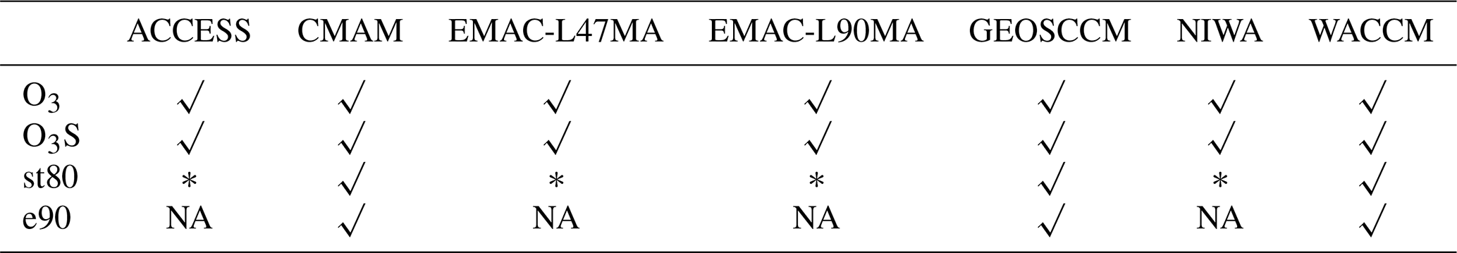
√: available. NA: not available. ∗: implementation issues.
The transport changes underlying the changes in stratospheric tracer concentration in the troposphere will be examined through the analysis of the TEM budget. The TEM tracer continuity equation can be written for the zonal mean tracer mixing ratio on pressure levels as follows (Andrews et al., 1987):
where is the eddy tracer flux vector. The subscripts indicate partial derivatives, (, ) are the residual circulation components, overbars indicate zonal mean and prime deviations from it, with a scale height H=7 km, R is the ideal gas constant, and the log-pressure altitude is with p0=1000 hPa. The chemical net tendency is given by the production minus loss term, . The resolved transport terms describe advection by the residual circulation, , and eddy transport, , related to two-way mixing. In addition to these resolved terms there is unresolved or subgrid-scale transport, which includes numerical diffusion and parameterized processes such as gravity waves and convection (). However, here we will focus on the main resolved transport terms, and we refer the reader to Abalos et al. (2017) for a detailed discussion of the other terms in the budget in WACCM. We note that daily mean data are needed to compute the TEM terms, for both the dynamical and chemical fields. This is not available in all models for the artificial tracers, so we only present the TEM budgets for which daily output was available.

Figure 1Time series of tropospheric columns of ozone (a), stratospheric ozone (b), st80 (c), and the ratio between O3 and O3S (d). Ozone and stratospheric ozone are plotted in Dobson units, while st80 is shown as standardized anomalies (removing the mean and dividing by the standard deviation).
3.1 Time series of tracer concentrations
Figure 1 shows time series over the 21st century of tropospheric columns of ozone (Fig. 1a), stratospheric ozone O3S (Fig. 1b) and the artificial tracer st80 (Fig. 1c), as well as the ratio of stratospheric to total ozone O3S∕O3 (Fig. 1d), for the REF-C2 simulations. The tropospheric tracer columns are based on the thermal tropopause, which is provided as an output for every model. This figure demonstrates that the concentration of stratospheric tracers in the troposphere will increase in the future, and this result is robust across the CCMI models. The total ozone concentration in the troposphere (Fig. 1a) increases in most models until the middle of the century and then decreases (except ACCESS and NIWA, which show a near constant decrease throughout the century). Comparing the total ozone to the stratospheric ozone evolution (Fig. 1a and b) it is clear that the future evolution of chemical production in the troposphere is crucial for future ozone concentrations. Although not shown here, we have confirmed that a sensitivity WACCM simulation with fixed tropospheric ozone precursor emissions (SEN-C2-fEmis) does not show a decrease in the second half of the century as is seen in Fig. 1a. In the IPCC scenario RCP6.0 under consideration, methane emissions increase until 2080 and then decrease, and nitrogen monoxide emissions decrease from 2000 and more rapidly in the second half of the century (not shown; see Meinshausen et al., 2011). The evolution of these gases is likely contributing to the tropospheric ozone column behavior in Fig. 1a. In contrast, Fig. 1b shows that stratospheric ozone (O3S) in the troposphere increases monotonically throughout the century, with a slight reduction of the concentrations over the 2 most recent decades in most models. This small reduction is linked to photochemical production of ozone from methane in the stratosphere, as we have confirmed by examining additional sensitivity runs of the model CMAM with methane emissions fixed to 1960 levels (not shown). The fraction of stratospheric to total ozone in the troposphere increases linearly in all models (Fig. 1d). In this sense, the models show a good qualitative agreement, although the ratio shows a large spread, from 22 % to 45 % for the year 2000. Trends in the ratio range from 0.32 % per decade to 0.99 % per decade among the models, with CMAM showing the largest trends and GEOSCCM the smallest. Note that the O3S increase is also seen in ACCESS and NIWA, which, when combined with the near flat trends in O3, leads to an increase in the stratospheric ozone fraction.
For st80 (Fig. 1c), the time series shown are standardized anomalies, i.e., the climatology is subtracted and the result is divided by the year-to-year standard deviation of the full time series, in order to focus the attention on the temporal evolution and not on the different magnitude of the concentration across the models. For instance, the magnitude of this artificial tracer in the EMAC models is notably smaller than in the rest (about 50 times), due to an implementation issue (see Sect. 2). However, the standardized anomalies show comparable values in Fig. 1c. The artificial tracer st80 shows an increase over the 21st century in all models except for NIWA and ACCESS. The evolution of st80 is very different in each of these two outliers, and cannot be reconciled with the increase seen in O3S in both models. For this reason, in the rest of the paper the st80 tracer will not be considered in these two models. As mentioned above, these two are essentially the same model. We emphasize here that the increase in st80 can be directly attributed to enhanced STT, excluding the contribution of changes in stratospheric ozone chemistry present in O3S. Specifically, an increase in stratospheric ozone is expected from stratospheric cooling and the continued decrease in halogens over the 21st century. In addition, note that the flattening of O3S time series towards the end of the 21st century linked to the evolution of methane in this scenario is not seen in st80.
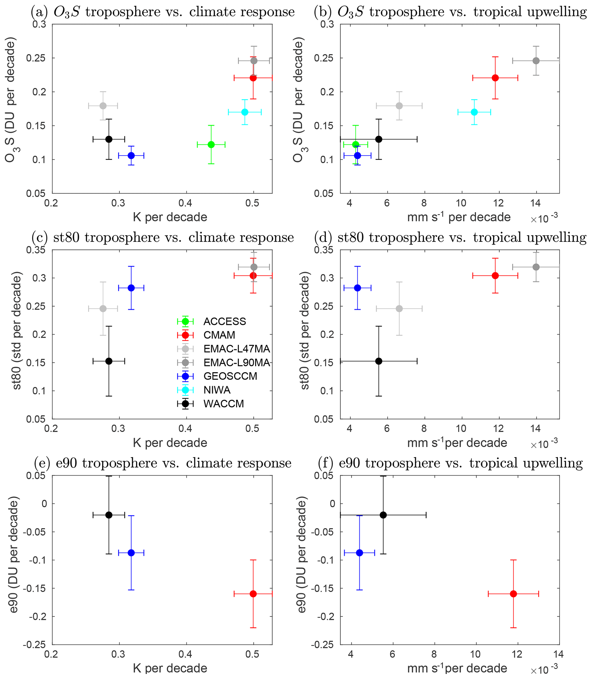
Figure 2Trends over the 21st century in globally integrated tropospheric columns of idealized tracers (a, b: O3; c, d: st80; e, f: e90) plotted against model climate response (a, c, e) and against tropical upwelling (b, d, f). Climate response is evaluated as the tropical upper troposphere temperature trend (30∘ S–30∘ N and 400–150 hPa); tropical upwelling is averaged over 100–70 hPa and 20∘ S–20∘ N. The error bars represent the trend uncertainty calculated with a Student t test with a 95 % confidence level.
Figure 2a and c show the trends in st80 and O3S tropospheric columns as a function of the climate response of each model, estimated as the rate of warming of the tropical upper troposphere (30∘ S–30∘ N, 400–150 hPa) under the RCP6.0 scenario. Note that we avoid using the term climate sensitivity because these simulations include several forcings in addition to CO2, for example, time-varying ODS. EMAC-L47MA (coupled ocean), GEOSCCM and WACCM have the smallest climate responses, and EMAC-L90MA (prescribed ocean) and CMAM have the largest responses. Although there is some spread, a relation between the two variables can be observed: models with a larger climate response tend to produce larger trends in STT, and this relation is more clearly seen for st80 than for O3S. Note that st80 trends are computed for the standardized time series, as shown in Fig. 1. The statistical significance of all trends in the paper is computed with a two-tail Student's t test for the slope at the 95 % confidence level (Storch and Zwiers, 1999).
Given the strong coupling between tropical upper tropospheric temperature and tropical upwelling, we can hypothesize that the BDC acts as a mediator between the climate response and STT. Figure 2b and d demonstrate this connection: models with stronger BDC acceleration produce stronger increases in STT for both stratospheric tracers. The transport mechanisms behind these correlations are discussed in the following sections. Overall we argue, based on the spatial structure of the tracer trends and TEM analyses, that zonal mean advective transport by the residual circulation plays an important role in driving STT trends.
In addition to the stratospheric tracers considered above, the evolution of a tropospheric artificial tracer provides a complementary view of the trends in stratosphere–troposphere exchange (STE). Figure 2e shows trends in the tropospheric tracer e90 in the troposphere for the three models that provide this output (CMAM, GEOSCCM and WACCM). The magnitude of the tracer trends increases with the climate response of the model. Note that there is a nonsignificant trend in WACCM, different from Fig. 13 in Abalos et al. (2017), which showed a significant decrease in the e90 concentrations averaged over the troposphere (in ppbv). However, we note that the difference in the trends in the tropospheric average in Abalos et al. (2017) versus those in the tropospheric column in Fig. 2c is not significant, since the 95 % confidence intervals overlap between the two. The other two models show a significant net decrease, larger for CMAM. The reduction of tropospheric tracer concentrations in the troposphere is consistent with a more efficient transport into the stratosphere, which is indeed related with stronger tropical upwelling in the future, as shown in Fig. 2f (see also, e.g., Rind et al., 2001; Abalos et al., 2017).
3.2 Spatial structure of the tracer trends
As a first step to understand the changes in transport processes leading to long-term trends in the STT rates seen in Figs. 1 and 2, in this section we examine the zonal mean spatial structure of the trends. We note that the trends in EMAC-L90MA are qualitatively very similar to those in EMAC-L47MA, and thus only the latter is shown in the rest of the paper, denoted as EMAC.
Starting with the tropospheric tracer, Fig. 3 shows the spatial structure of the trends in e90. The three models yield highly consistent results, and the magnitude scales with the climate response shown in Fig. 2e. Using the TEM formalism, Abalos et al. (2017) examined the causes leading to these trend patterns, showing that they reflect known effects of climate change. The increase in the tropical lower stratosphere is attributed to enhanced BDC tropical upwelling, while the increases in the extratropical upper troposphere–lower stratosphere (UTLS) are at least partly linked to enhanced isentropic mixing in this region. The rise of the tropopause with climate change plays a key role in these changes, as it implies an upward shift of the regions of wave dissipation and therefore an upward shift of the residual circulation wave forcing (Oberländer-Hayn et al., 2016) and isentropic mixing (Abalos et al., 2017). In addition, as the troposphere expands, the composition of the UTLS becomes more troposphere-like, since tracers encounter the change in transport regime defined by the tropopause at higher levels. In the extratropical troposphere, the negative trends are associated with weaker meridional mass circulation and isentropic mixing. In the tropical troposphere, they are consistent with more intense and deeper circulation in the upper part of the Hadley cell, linked to enhanced deep convection and connected to the stronger BDC tropical upwelling. In simple terms, the reduction in the tropospheric e90 concentrations reflects a less efficient transport from the surface into the extratropical free troposphere and a more efficient (tropical) troposphere-to-stratosphere transport in the future.
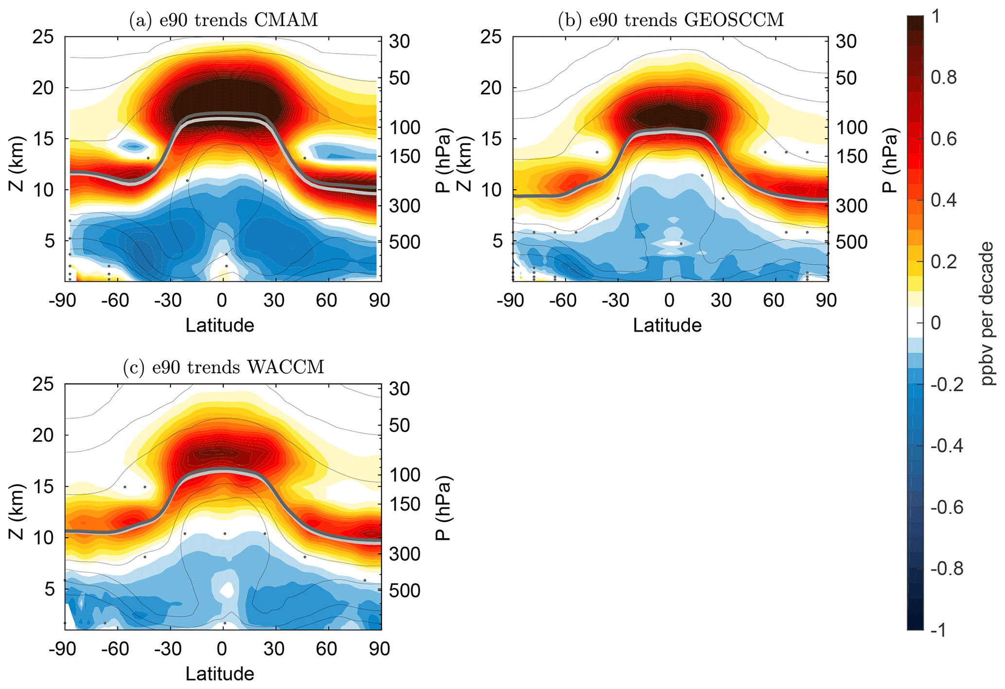
Figure 3Trends over the 21st century in e90 (ppbv per decade). The dotted regions indicate where the trends are not statistically significant for a 95 % confidence level. The light and dark gray lines indicate the location of the tropopause in the decades of the 21st century, respectively. Thin black contours show the climatological concentrations of e90 (contour correspond to values of 0.1, 1, 10, 100, 110, 120 and 130 ppbv). Note that Z is the log-pressure altitude , with H=7 km and p0=1000 hPa in this figure and in all other cross sections.
The trends in O3S are shown in Fig. 4. In the stratosphere, ozone decreases in the tropics and increases in the extratropics, and this pattern is expected from the acceleration of the residual circulation seen in all models (as will be shown below). There is an interhemispheric asymmetry in the lowermost stratosphere, with stronger positive trends in the Southern Hemisphere (SH) extending to lower levels than in the Northern Hemisphere (NH). Only in two models, EMAC and GEOSCCM, are there positive trends around the NH extratropical tropopause. This is probably due to the dominant effects of ODS over GHG in these two models, as will be argued in Sect. 5. The large SH O3S positive trends are due to the recovery of the Antarctic ozone hole. In contrast, the negative trends around the NH extratropical tropopause are consistent with trends in the artificial tracer e90 identified in Fig. 3 (in both hemispheres). As stated above, these trends around the extratropical UTLS constitute a fingerprint of the tropopause rise. This is confirmed by looking at the tracer trends in tropopause-relative coordinates, in which the bands around the extratropical tropopause are not present, as shown for e90 in Fig. 8 of Abalos et al. (2017). The same is true for O3S (not shown). The change in tropopause altitude as a function of latitude over the 21st century is shown in Figs. 3, 4 and 5. In the troposphere, O3S trends are positive, and their spatial structure reveals a common pattern across models (Fig. 4). The largest trends are found in the subtropics, near 30∘ N/S in the middle to upper troposphere (∼500–200 hPa). The positive trends extend to higher latitudes below the tropopause, and these extratropical increases are stronger in the SH than in the NH in all models. The deep tropics display a local minimum and near-zero trends or even negative trends are found next to the ground in the tropics, consistent with little influence of stratospheric air in these regions. This pattern is consistent with those shown by Banerjee et al. (2016) and Meul et al. (2018) in individual models.
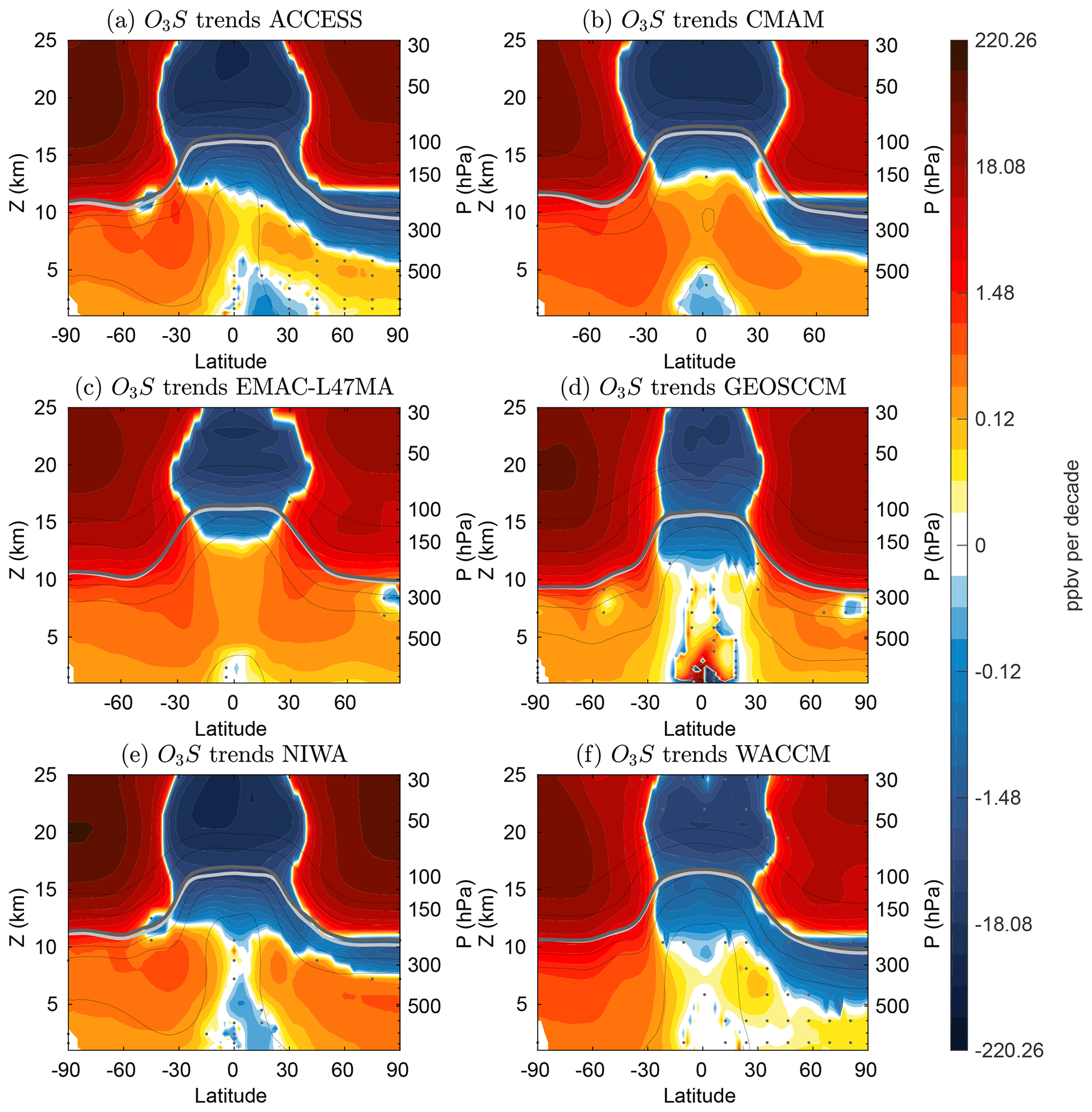
Figure 4Trends over the 21st century in stratospheric ozone (ppmv per decade, in logarithmic scale). The dotted regions indicate where the trends are not statistically significant for a 95 % confidence level. The light and dark gray lines indicate the location of the tropopause in the first and last decades of the 21st century, respectively. Thin black contours show the climatological concentrations of O3S (contour levels shown correspond to 10, 50, 100, 500 and 1000 ppbv).
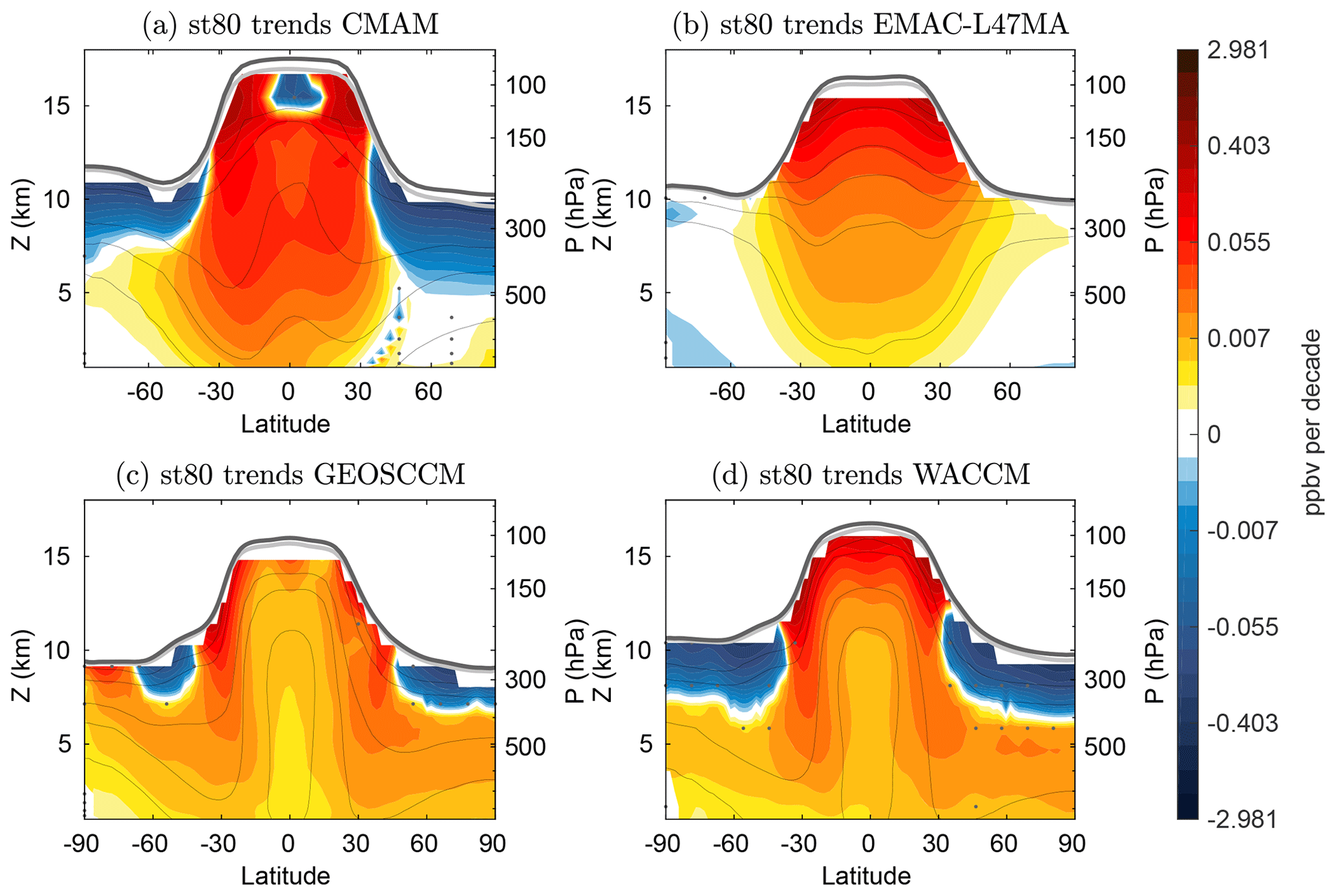
Figure 5Trends over the 21st century in stratospheric tracer st80 (ppbv d−1, in logarithmic scale). The dotted regions indicate where the trends are not statistically significant for a 95 % confidence level. The light and dark gray lines indicate the location of the tropopause in the first and last decades of the 21st century, respectively. Thin black contours show the climatological concentrations of st80 (contour levels correspond to 0.1, 0.25, 0.5, 1, 5 and 10 ppbv).
In Fig. 5 we use the artificial tracer st80 in order to examine the trend patterns for an artificial tracer with constant and homogeneous stratospheric sources. Note that this tracer is only useful in the troposphere, since it has a constant fixed value of 200 ppbv at and above 80 hPa, and thus the stratospheric values are not shown. The st80 trends in EMAC (Fig. 5b) have been multiplied by an arbitrary factor of 50 in order to fit the scale due to a known implementation issue (see Sect. 2). The st80 trends in Fig. 5 show more hemispherically symmetric patterns as compared to Fig. 4, with negative trends near the extratropical tropopause in both hemispheres (except in EMAC), as seen in the NH trends for O3S and consistent with e90 trends in Fig. 3. In addition, there are positive trends maximizing in the subtropical troposphere in both hemispheres that extend to higher latitudes below the region of negative trends linked to the extratropical tropopause. This structure is similar to that seen for O3S, although not exactly comparable due to differences in the gradients between these two tracers and their different stratospheric source distributions (see climatology contours in Figs. 4 and 5).
In the deep tropical upper troposphere, all models show a local minimum, although CMAM and EMAC show higher concentrations at the Equator than GEOSCCM and WACCM. Note that the former models also show higher climatological st80 concentrations in the deep tropics, suggesting leakier tropical tropopauses in these models. As the tropopause rises in the simulated future climate, it gets closer to the source level of st80 (80 hPa), and vertical transport into the tropical troposphere is enhanced. This effect is magnified in models with a higher tropopause, such as CMAM (Fig. 5a).
Overall, the O3S and st80 trend patterns highlight common features in all models, and in the next section we investigate the transport changes that lead to these trends in the stratospheric tracers.
To facilitate interpretation of the TEM transport terms that will be shown next, Fig. 6 shows the trends in the residual circulation streamfunction for the various models included in this study. In the stratosphere, all models show an acceleration of the BDC in both hemispheres. However, while in the NH the acceleration extends from the tropics to polar latitudes, in the SH there is a cell of opposite sign at high latitudes. This is due to the impact of the ozone hole recovery on the residual circulation. Specifically, the ozone recovery weakens the downwelling in the SH high latitudes over the 21st century, reversing the acceleration induced during the ozone hole formation over the last decades of the 20th century (Polvani et al., 2018; Abalos et al., 2019). This behavior is observed in most CCMI models (Morgenstern et al., 2018; Polvani et al., 2019). Figure 6 confirms this common behavior, with EMAC being an exception with near-zero residual circulation trends in the SH polar latitudes. The fact that this feature does not appear as clearly in this model could be linked to a weak SH polar vortex.
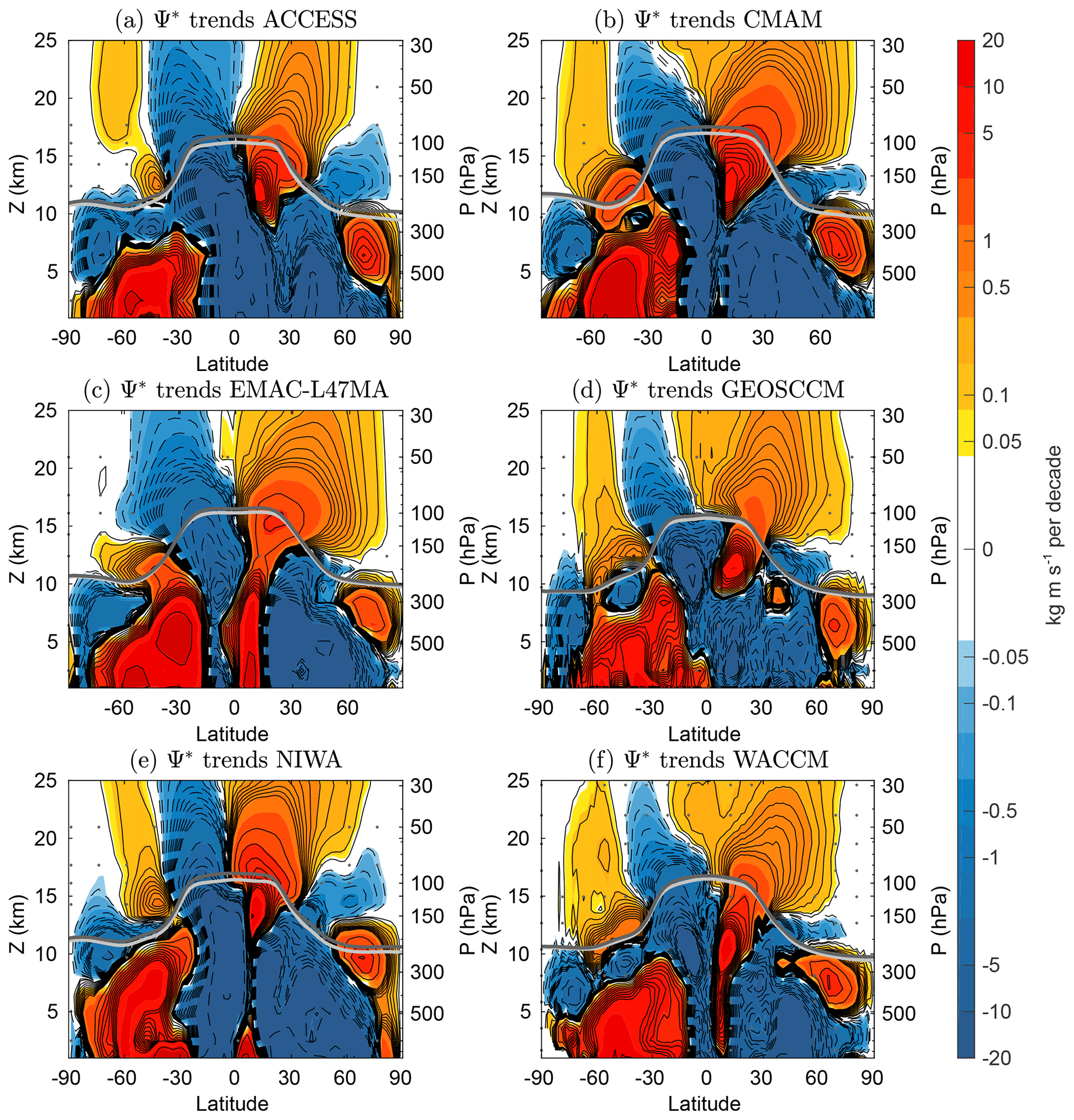
Figure 6Trends over the 21st century in residual circulation streamfunction. The dotted regions indicate where the trends are not statistically significant for a 95 % confidence level. The light and dark gray lines indicate the location of the tropopause in the first and last decades of the 21st century, respectively.
In the troposphere, most models show a deceleration of the residual circulation in the extratropics of both hemispheres. In the tropics, all models show a strengthening of the upper part of the Hadley cell, just below the acceleration of the shallow branch of the stratospheric circulation. As shown in Abalos et al. (2017), this strengthening is closely linked to the upward shift of the tropopause. As will be shown below, the enhanced downwelling of the Hadley cell in the upper subtropical troposphere cooperates with the enhanced shallow branch of the BDC to enhance advective downward transport of the stratospheric tracers into the troposphere. This leads to the subtropical upper tropospheric maxima in the O3S and st80 trend patterns seen in Figs. 4 and 5. Moreover, Fig. 6 demonstrates that this mechanism is present in all models.
Figures 7 and 8 show the 21st century change in the advective transport term for the tracers O3S and st80, respectively, in four models (CMAM, EMAC, GEOSCCM and WACCM). We note that the daily output for CMAM was obtained 3 times per month, while the other models had output for every day of the year. In order to increase the amount of data in CMAM, we considered differences between the first and last half of the century for this model. For the others, differences between the first and last decade of the century are considered.
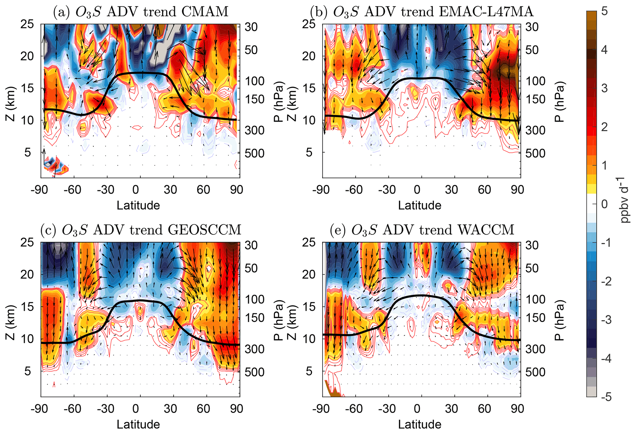
Figure 7Change over the 21st century in the O3S TEM advective transport term (shading, ppbv/d) in CMAM (a), EMAC-L47MA (b), GEOSCCM (c) and WACCM (d). The arrows show the residual circulation components multiplied by the absolute value of the corresponding tracer gradient. The red and blue contours are spaced by 0.1 and go up to ±0.5 ppbv d−1.
The O3S advective term (Fig. 7) shows a decrease in the concentrations in the tropical lower stratosphere due to enhanced upwelling, and increases at extratropical latitudes due to enhanced downwelling. At polar latitudes in the SH, we see the effects of ozone hole recovery, which are twofold: an increase in O3S concentrations in the polar lower stratosphere, and a weakening of the residual circulation polar downwelling (seen in Fig. 6; see also Polvani et al., 2018). The latter dominates above ∼20 km, resulting in negative trends in advection of O3S. Below 20 km, the ozone recovery due to decreasing ODS dominates, and the net effect is an increase in ozone downward transport. As a result, there is enhanced advective STT of stratospheric ozone at polar latitudes in both hemispheres, due to a larger reservoir in the lowermost stratosphere (and not to stronger downwelling across the tropopause; see Fig. 6). In the NH, the enlarged lower stratospheric ozone reservoir is partly due to the acceleration of the deep branch of the BDC (Fig. 7). In the SH, where the BDC actually decelerates, it is exclusively due to reduced photochemical destruction as ODS concentrations decline.
All models show positive trends in ozone due to advection near the subtropical tropopause (approximately 30∘ N and 30∘ S at 150 hPa). The arrows indicate an enhancement of the amount of stratospheric ozone being advected across the tropopause into the troposphere in these regions by the enhanced shallow branch of the BDC and top of the Hadley cells. These patterns lead to the subtropical tongues observed in the O3S trends in Fig. 4. Hence, both shallow and deep branches of the BDC lead to enhanced stratospheric ozone transport into the troposphere.
Figure 8 shows the advective transport term for the artificial tracer st80 in the same four models. Again, all models show consistent features. In particular, similar to the behavior seen in O3S, there is enhanced downward transport into the troposphere in the subtropics linked to the shallow BDC and top of the Hadley cell. These patterns lead to the subtropical tongues in the st80 trends seen in Fig. 5. Note that the tongue structure is somewhat different in the two tracers, due to the different background gradients (compare the climatological concentrations in Figs. 4 and 5). At polar latitudes in the NH, GEOSCCM and WACCM show enhanced downward transport into the troposphere. This is consistent with lower stratospheric reservoir enlargement of st80 by the enhanced downwelling of the deep branch, as seen for O3S. The fact that CMAM and EMAC-L47MA fail to capture these trends reflects issues with the st80 idealized tracer concentrations in the stratosphere (see Orbe et al., 2018, Fig. S2 in their Supplement). In particular, these two models do not show an increase in st80 concentrations in the NH lower stratosphere, as would be expected from the strengthened BDC. On the other hand, the fact that none of the models show enhanced downward transport of st80 at SH polar latitudes confirms that the enlarged O3S reservoir and subsequent enhanced STT in this region seen in Fig. 7 is exclusively linked to ozone recovery.
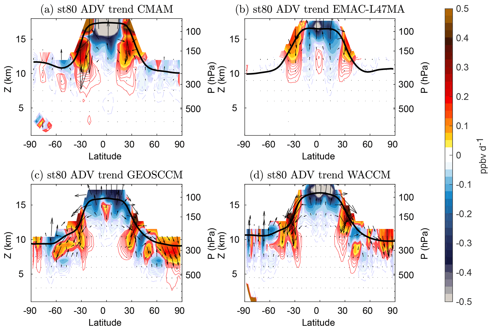
Figure 8Change over the 21st century in the st80 TEM advective transport term (shading, ppbv/d) in CMAM (a), EMAC-L47MA (b), GEOSCCM (c) and WACCM (d). The arrows show the residual circulation components multiplied by the absolute value of the corresponding tracer gradient. The red and blue contours are spaced by 0.005 and go up to ±0.05 ppbv d−1.
While we find good correspondence among models in the advective transport term (Figs. 7 and 8), the eddy mixing term is subject to larger uncertainties and there is a larger spread among models. This term is computed from meridional and vertical eddy tracer fluxes (see Eq. 1 and related discussion), which are highly sensitive to numerical errors arising from different sources, including limited temporal resolution of the output, implicit diffusion in the model transport scheme and vertical interpolations (see Abalos et al., 2017 for a discussion of these errors in WACCM). Since understanding the sources of uncertainty in each model in detail is beyond the scope of the study and our goal is to extract robust trend features in the transport terms, we only include results for models showing consistent behavior. At the same time, we warn that the conclusions extracted for the eddy term should be considered more uncertain than those found for the advective term, given the limited inter-model agreement.
Figure 9 shows the trends in the eddy term for O3S (Fig. 9a and b) in CMAM and WACCM and for st80 in GEOSCCM and WACCM (Fig. 9c and d). In the stratosphere there is enhanced isentropic mixing transporting O3S from high latitudes into the tropics in both models and enhanced eddy transport out of the SH polar stratosphere. Of greater interest for this study are the trends in cross-tropopause transport. For both tracers there is enhanced isentropic mixing across the extratropical tropopause, which leads to increases in ozone concentrations in the upper troposphere middle latitudes in both hemispheres (30–60∘ N/S). In addition to increasing the tropospheric concentrations, this enhanced eddy transport decreases the tracer concentrations in the lowermost extratropical stratosphere. This is consistent with the enhanced isentropic eddy transport in e90 found by Abalos et al. (2017), leading to the increased concentrations in this tracer around the extratropical tropopause (Fig. 3). Hence, the same mechanism likely contributes to the negative trends in st80 and O3S (only in the NH) around the extratropical tropopause (Figs. 4 and 5). This is added to the direct effect of the tropospheric expansion on the extratropical UTLS composition, as mentioned in Sect. 3.2.
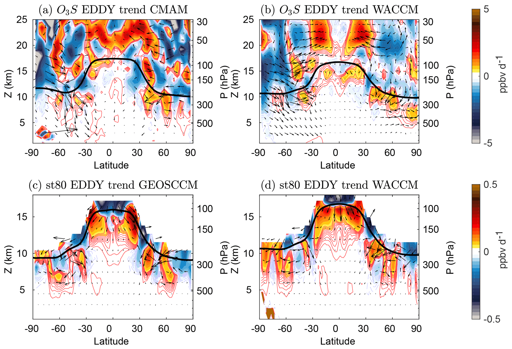
Figure 9Change over the 21st century in the st80 TEM eddy transport term (shading, ppbv/d) in CMAM (a), EMAC-L47MA (b), GEOSCCM (c) and WACCM (d). Arrows denote the direction and magnitude of the eddy tracer flux. In panels (a, b) the red and blue contours are spaced by 0.1 and go up to ±0.5 ppbv d−1. In panels (c, d) the red and blue contours are spaced by 0.005 and go up to ±0.05 ppbv d−1.
Finally, there is enhanced cross-tropopause near-vertical transport of st80 in the tropics, which contributes to enhancing the concentrations in the tropical upper troposphere on both sides of the Equator. This feature is mainly due to the fixed st80 concentrations above 80 hPa: as the tropical tropopause rises and gets close to this level, vertical gradients strengthen and lead to cross-tropopause transport.
Note that we do not attempt to provide a quantitative estimate of the contribution from each transport term to the net tracer trends. The total balance should include additional transport terms, such as convection, diffusion and transport by subgrid-scale waves, as well as the chemical tendency term (important for O3S). Even if those terms were considered the budget would not be exactly closed, due to the numerical issues such as those listed in Abalos et al. (2017), which are model dependent. Nevertheless, the two resolved transport terms provide valuable information on the different effects of these transport mechanisms on the tracer trends. Specifically, Figs. 7 to 9 suggest that the trend patterns seen in O3S and st80, particularly in the subtropics and at polar latitudes, result from enhanced advective transport into the troposphere. The relevance of the mean advection by the stratospheric residual circulation and the upper part of the Hadley cell for the STT trends is a novel result that has not been considered before.
These results shown up to now apply for the RCP6.0 scenario of the IPCC, but, as mentioned in the Introduction, other scenarios may lead to different results. Figure 10 shows time series of tropospheric columns of various stratospheric tracers over the 21st century by comparing the RCP6.0 to the RCP8.5 scenarios. These data are only available in three models: CMAM, EMAC-L47MA and WACCM. Figure 10a reveals a clear difference in the evolution of ozone in the troposphere, which increases throughout the century in the RCP8.5 scenario in the three models and decreases in the RCP6.0 scenario. Part of this difference in the evolution of ozone could be explained by differences in the precursor emissions between the two scenarios. Methane increases monotonically throughout the century in the RCP8.5 scenario, while in the RCP6.0 scenario it increases at a much slower rate and then decreases during the last 2 decades of the century (Meinshausen et al., 2011). In contrast, nitrogen monoxide emissions decrease over the 21st century in the two scenarios, with similar slopes (not shown), thus they cannot explain the differences. In addition to these chemical effects, the stronger acceleration of the BDC in the more extreme scenario leads to enhanced ozone STT when compared to the other scenario. The connections established in previous sections the present study between the BDC acceleration and STT suggest that this dynamical effect is important. Finally, there could be a contribution from the faster rate of stratospheric ozone recovery due to larger stratospheric cooling in RCP8.5 (WMO, 2018). Overall, we argue that both chemical and dynamical effects contribute to the fast increase in tropospheric ozone in RCP8.5 (absent in RCP6.0).
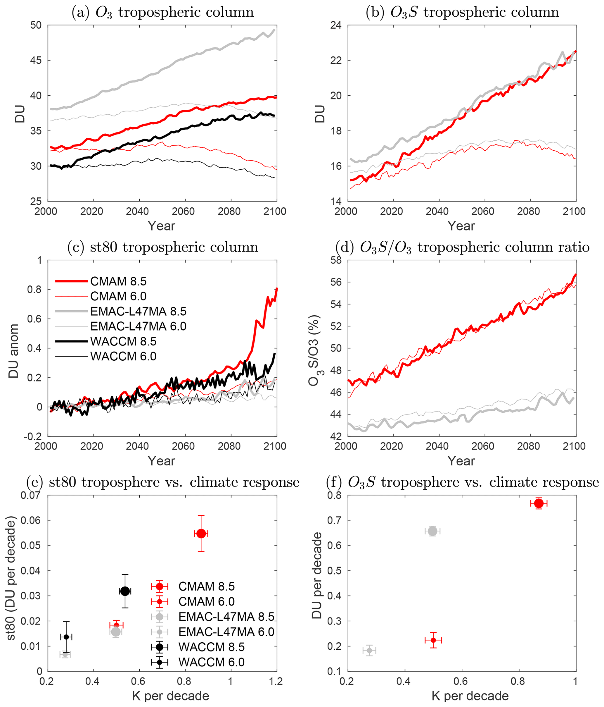
Figure 10(a–d) Time series of tropospheric column tracers for the RCP8.5 (thick lines) and RCP6.0 (thin lines) scenarios. The st80 concentrations are expressed as anomalies with respect to the average of the first decade, and the values for EMAC-L47MA are multiplied by an arbitrary factor of 50 (see text for details). (e, f) Trends in tropospheric column tracers versus model climate response for the RCP8.5 (large circles) and the RCP6.0 (small circles) scenarios. The error bars represent the trend uncertainty with a 95 % confidence level. Note that the O3S tracer is not available in the RCP8.5 WACCM simulation.
Consistent with a larger increase in ozone STT, O3S increases faster in the more extreme scenario (Fig. 10b). The largest difference between the two scenarios for this tracer is seen in the last 20 years of the simulations, where O3S concentrations remain flat in RCP6.0 but continue to increase in RCP8.5. As mentioned in Sect. 3.1, this flattening of O3S in RCP6.0 is related to reduced ozone production from methane in the lower stratosphere. There is no significant difference in the ratio of stratospheric to total ozone between the two scenarios (Fig. 10d). For st80 (Fig. 10c), there is a steady increase in the RCP8.5 for all models that is larger than in the RCP6.0 scenario. In CMAM this increase is particularly enhanced over the last 20 years, perhaps due to the tropical tropopause being close to 80 hPa by the end of the century. The 21st century trends in O3S and st80 in the two scenarios are compared in Fig. 10e and f. In all models the climate response is stronger in the higher emissions scenario, and the tracer trends are significantly (2–3 times) stronger, consistent with more severe climate change and associated transport changes. We note that considering the trends until 2080 does not alter the substantial difference found between the two scenarios.
Polvani et al. (2018) showed that the future acceleration of the BDC due to the increase in GHG is partly compensated for by the decrease in ozone-depleting substances (ODS). More specifically, they showed that the global mean age of air trends in the 21st century are reduced by about half with respect to those observed over the last few decades of the 20th century. The main reason for this decrease is the weakening of the polar SH downwelling associated with the recovery of the ozone hole. Here, we examine the separate contributions to the STT trends from changes in the GHG and ODS emissions. Banerjee et al. (2016) and Meul et al. (2018) examined the impact of these two forcings on ozone transport into the troposphere in individual models and found that increases in GHG lead to increases in stratospheric ozone in the subtropics, while ozone recovery leads to ozone enhancement at higher latitudes.
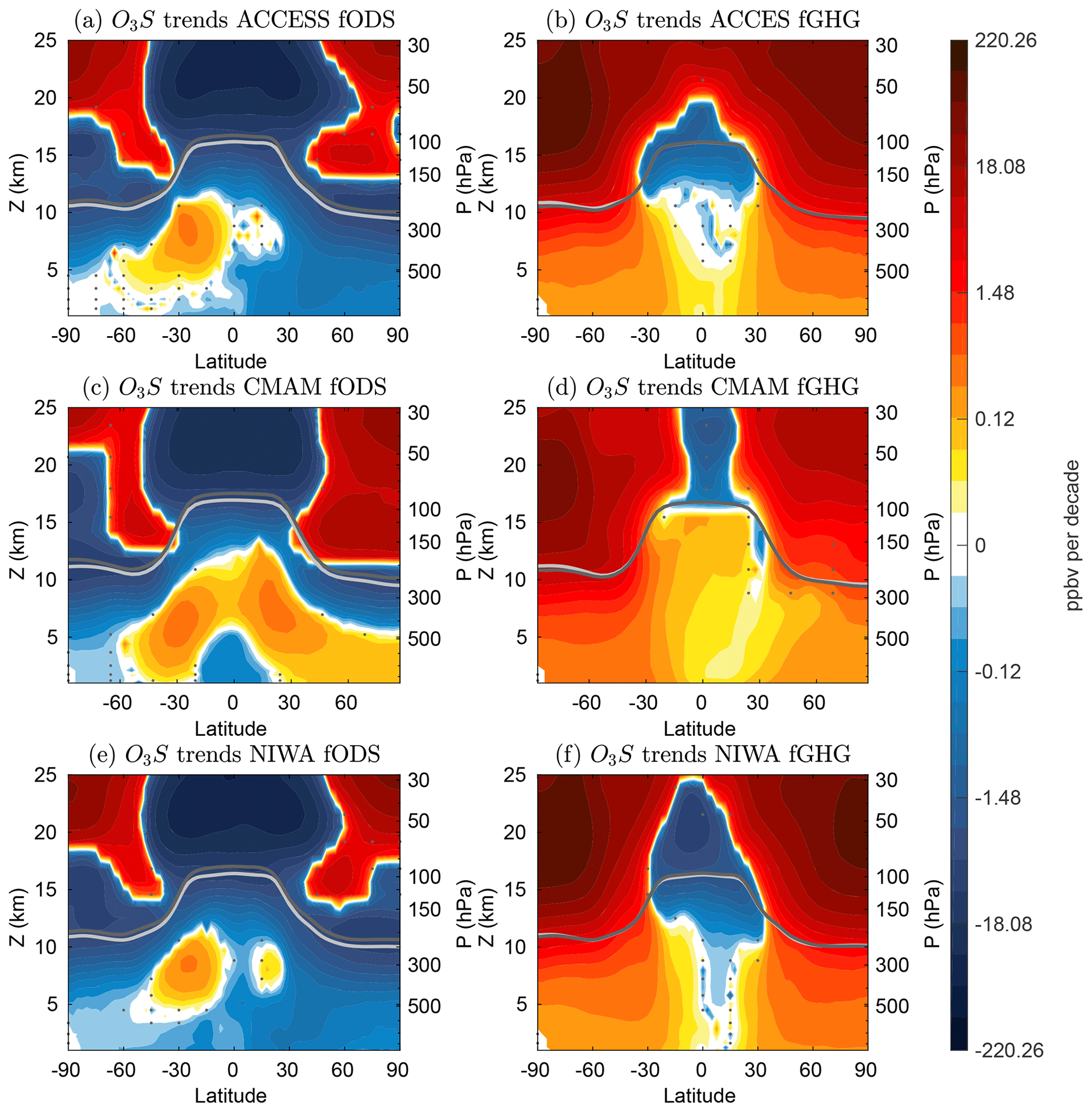
Figure 11Trends over the 21st century in O3S (ppbv per decade) for the simulations with ODS (a, b) or GHG (c, d) concentrations fixed to 1960 levels in ACCESS (a, c) and CMAM (b, d). The dotted regions indicate where the trends are not statistically significant for a 95 % confidence level. The light and dark gray lines indicate the location of the tropopause in the first and last decades of the 21st century, respectively.
Figure 11 shows the trends in O3S for the three models that output this tracer (ACCESS, CMAM and NIWA) for sensitivity simulations with concentrations of ODS or GHG fixed to 1960 levels. Since we are looking at trends for the 21st century, the fixed-ODS simulations can be conceptualized as characterizing the impact of the increase in GHG through the century, and the fixed-GHG simulations as characterizing the impact of the elimination of halogens. Comparing Fig. 11a, c and e with Fig. 4 it is clear that increases in stratospheric ozone in the troposphere are more modest when ODS concentrations are fixed. This reflects the fact that stratospheric ozone recovery leads to more ozone being transported into the troposphere. In agreement with previous studies, in the fixed-ODS simulations the O3S increases are limited to the subtropical region. The negative trends near the extratropical tropopause are consistent with the changes associated with the tropopause rise in response to climate change mentioned above (Figs. 3–5, Abalos et al., 2017). It becomes evident now that the band of negative O3S trends in the NH extratropical UTLS seen in Fig. 4 is due to the effect of GHG increases, while ODS increases yield positive O3S trends in this region. Consistently, we conclude that in the two models that do not show such band of negative trends, EMAC and GEOSCCM, the stratospheric ozone recovery overwhelms the GHG effect (Fig. 4c and d). Note that we cannot provide exact proof of this conclusion because we do not have fixed ODS or fixed GHG simulations for those two models in particular.
The differences between the control and sensitivity simulations are especially evident in the SH, where the ozone hole is located and thus the ozone recovery effect is the strongest. This effect of ozone recovery is isolated in the fixed-GHG sensitivity simulations (Fig. 11b, d and f). These clearly show that increases in stratospheric ozone concentrations result in increased STT mostly in the extratropics. The results in Fig. 11 are highly consistent with those from previous studies highlighted above (Banerjee et al., 2016; Meul et al., 2018). Analysis of the time series of globally integrated O3S tropospheric columns for the REF-C2, SEN-C2-fODS and SEN-C2-fGHG simulations (not shown) reveals that, in ACCESS and NIWA, the increase in O3S STT is dominated by the effect of ozone recovery. In contrast, in CMAM both GHG and ODS contribute approximately the same to the net trends in O3S STT. Thus, there is no agreement in the relative contributions of these two external forcing to STT increases for O3S.
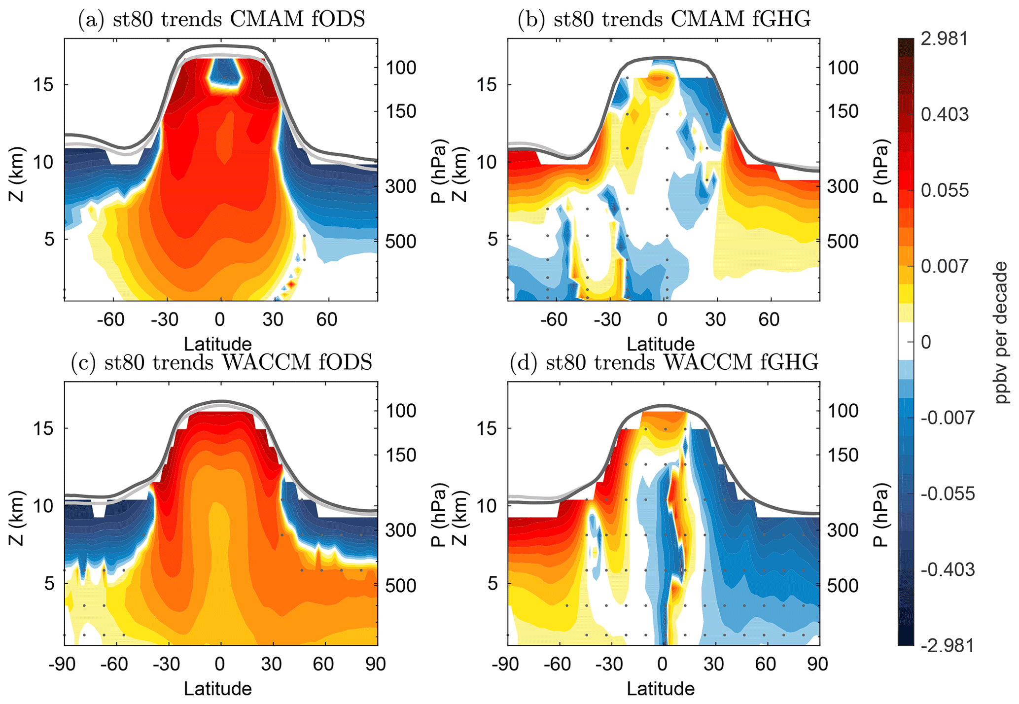
Figure 12Trends over the 21st century in st80 for the simulations with ODS (a, b) or GHG (c, d) concentrations fixed to 1960 levels in CMAM (a, c) and WACCM (b, d). The dotted regions indicate where the trends are not statistically significant for a 95 % confidence level. The light and dark gray lines indicate the location of the tropopause in the first and last decades of the 21st century, respectively.
In order to separate the effects of changes in transport from those of stratospheric ozone recovery, we now look at st80 trends. Figure 12 shows trends in the sensitivity simulations for st80 in CMAM and WACCM (note that ACCESS and NIWA are not used for the reasons explained in Sect. 3.1). In contrast to O3S, the st80 trends in the fixed-ODS runs (Fig. 12a and c) are very similar to those in the control simulations for both models, not only in the subtropics but also at high latitudes (Fig. 5). This confirms that the changes in transport mechanisms examined in the previous section are mainly caused by the increase in GHG. On the other hand, the trends in the fixed-GHG simulations (Figs. 12b and d) are much more uncertain and are statistically insignificant over large regions of the troposphere. For instance, the two models show opposite sign trends in the NH (not significant in WACCM and not consistent among 3 different members, not shown). This difference between the O3S and st80 trends in the fixed-GHG scenario confirms that the trends in O3S are due to the increase in ozone concentrations directly associated with ODS decline through changes in photochemistry, rather than by dynamical changes induced by ODS decline. Nevertheless, one consistent feature in the two models is the increase in st80 concentrations in the SH high-latitude upper troposphere (Fig. 12b and d). This is linked to a small downward shift of the tropopause in these simulations associated with the weakening of polar downwelling, a dynamical effect of the recovery of the Antarctic ozone hole (Polvani et al., 2018, 2019). Note that this SH tropopause shift is opposite to that associated with GHG increases (compare the tropopauses in Fig. 12a, c to b, d). Consistently, the positive st80 trends due to ozone recovery near the SH tropopause partly offset the decrease due to increasing GHG (the net result is still a decrease, as shown in Fig. 5). Besides this specific feature, no robust conclusion can be extracted for future changes in STT if GHG concentrations are fixed. The dominant role of climate change on the st80 STT trends is further confirmed for both models by comparing time series for the two fixed-forcing simulations in Fig. 12 to the all-forcing (REF-C2) runs (not shown).
In this study we investigated the future trends in stratosphere–troposphere exchange (STE), with a specific focus on stratosphere-to-troposphere transport (STT), using output from various models participating in CCMI in order to extract robust signals. Idealized tracer data provides a unique opportunity to evaluate changes in transport, separated from changes in chemical processes due, for instance, to changes in precursor concentrations. We show that all models agree in predicting an enhancement of the concentrations of stratospheric tracers in the troposphere in the future. The models project a near-linear increase in the fraction of stratospheric to total ozone in the troposphere between 10 % and 20 % over the 21st century with respect to the 2000–2010 mean values. This increase reflects the combined effects of increased transport – the tropospheric column of stratospheric ozone increases 10 %–16 % – and reduced chemical production in the troposphere during the second half of the 21st century in the RCP6.0 emission scenario considered here. These results are consistent with previous studies using individual models. Our multi-model approach allows for extracting a correlation between the climate response, the strength of the BDC and the magnitude of the STT trends in the different models.
In addition to ozone and stratospheric ozone (O3S), we analyze the idealized tracer st80, which is independent of chemistry in the stratosphere and in the troposphere. The patterns of trends in O3S and st80 exhibit common features, revealing the fingerprints in the tracer trends of changes in transport alone, excluding changes in stratospheric ozone chemical sources and sinks. One of the key features identified in the tracer trends are maximum increases in the subtropical troposphere of both hemispheres. In addition, the positive trends extend to high latitudes in the lower troposphere (below approximately 400 hPa). Negative trends are generally observed around the extratropical tropopause, except for O3S in the SH, where stratospheric ozone recovery leads to an increase in the concentrations across the tropopause.
The TEM tracer continuity equation is used to evaluate of the changes in transport processes leading to the enhanced STT, separating advective transport by the residual circulation from eddy transport, linked to two-way mixing. We find that enhanced advective transport plays a key role in the subtropical trend maxima for both O3S and st80. This is linked to the acceleration of the shallow branch of the residual circulation and the strengthening of the top of the Hadley cell. Note that the Hadley cell strengthening does not extend into the lower troposphere (see Fig. 6). This is consistent with recent studies arguing that metrics of the Hadley cell should be considered separately for the upper and lower parts (Davis and Davis, 2018; Waugh et al., 2018).
Enhanced downward advective transport due to the acceleration of the deep branch of the BDC contributes to STT over polar latitudes in the NH only, by accumulating the tracers in the “middle world” reservoir. In the SH, the dynamical effects of ozone hole recovery prevail and there is a weakening of polar downwelling (Polvani et al., 2018). Nevertheless, STT of O3S increases due to the higher ozone concentrations in the lower stratosphere as ODS declines.
Although larger uncertainties are obtained for the eddy transport term, a consistent feature identified is an enhancement of eddy transport in the extratropical UTLS. A similar feature was observed for the tropospheric tracer e90 by Abalos et al. (2017) and was linked to the rise of the extratropical tropopause and associated upward shift of the region of wave dissipation. These changes in mixing likely contribute to the negative trends in the stratospheric tracers around the extratropical tropopause, in addition to the direct effects of the upward expansion of the troposphere. Certainly, the rise of the tropopause is key to explaining these extratropical UTLS trends, which disappear when tropopause-relative coordinates are used.
While the same qualitative results apply when the more extreme scenario RCP8.5 is considered, the tropospheric column of stratospheric ozone increases 40 %–50 % by the end of the 21st century (with respect to the 2000–2010 mean values). This implies an increase more than 3 times larger than in the RCP6.0 scenario. However, this result is based on two models, due to limited availability of output. The results for st80 also suggest a larger increase for the high-emission scenario: the models show 2–3 times larger trends in the RCP8.5 scenario. Finally, we also explore the roles of two key forcings, GHG and ODS, separately. Using O3S, Banerjee et al. (2016) and Meul et al. (2018) showed that increasing GHG leads to enhanced stratospheric ozone in the subtropical troposphere, while ozone recovery leads to more modest enhancements throughout the extratropics. Here we confirm that this is also the case for all the models providing the specific sensitivity simulations. Moreover, using the idealized tracer st80 we show that the robust STT trends are primarily attributed to increasing GHG emissions. Ozone recovery (or ODS reduction) does not drive consistent trends in STT across models. However, in two out of the three available models, ozone recovery is mainly responsible for the observed increase in ozone STT into the troposphere. This apparent contradiction is simply explained by the fact that such an increase in ozone STT is due to stratospheric ozone photochemistry and not to changes in transport processes. However, these relative roles of GHG and ODS could be different in the more extreme climate change scenario, and this cannot be addressed with the current model output.
The assessment of future STT trends is key for interpreting future evolution in tropospheric ozone, and the present study demonstrates the usefulness of idealized tracers to better constrain transport changes. At the same time, we emphasize that tropospheric chemistry, and the evolution of precursor emissions in each scenario in particular, remains a major source of uncertainty.
The CCMI output data can be downloaded from the Centre for Environmental Data Analysis (CEDA): http://data.ceda.ac.uk/badc/wcrp-ccmi/data/CCMI-1/output/ (last access: April 2020, CEDA, 2020). CESM1-WACCM data can be downloaded from https://www.earthsystemgrid.org (last access: April 2020, NCAR, 2020). For instructions for access to both archives, see http://blogs.reading.ac.uk/ccmi/badc-data-access (last access: April 2020, CCMI, 2020).
MA wrote the manuscript and carried out the analyses. CO and DEK contributed with additional simulations. All coauthors contributed with discussions, expertise on the models and comments on the draft.
The authors declare that they have no conflict of interest.
This article is part of the special issue “Chemistry–Climate Modelling Initiative (CCMI) (ACP/AMT/ESSD/GMD inter-journal SI)”. It is not associated with a conference.
This study has been partly carried out using the high-performance computing and storage facilities provided by CISL/NCAR. The EMAC simulations have been performed at the German Climate Computing Center (DKRZ) through support from the Bundesministerium für Bildung und Forschung (BMBF). DKRZ and its scientific steering committee are gratefully acknowledged for providing the HPC and data-archiving resources for the consortial project ESCiMo (Earth System Chemistry integrated Modelling). We acknowledge the UK Met Office for use of the MetUM. This research was supported by the New Zealand Government's Strategic Science Investment Fund (SSIF) through the NIWA programme CACV. Olaf Morgenstern acknowledges funding by the New Zealand Royal Society Marsden Fund (grant 12-NIW-006). The authors wish to acknowledge the contribution of NeSI high-performance computing facilities to the results of this research. New Zealand's national facilities are provided by the New Zealand eScience Infrastructure (NeSI) and funded jointly by NeSI's collaborator institutions and through the Ministry of Business, Innovation, and Employment's Research Infrastructure programme (https://www.nesi.org.nz/, last access: April 2020). The GEOSCCM is supported by the NASA MAP program, and the high-performance computing resources were provided by the NASA Center for Climate Simulation (NCCS). The authors are grateful to the editor and the referees for the insightful reviews that contributed to notably improve the paper.
Marta Abalos acknowledges funding from the Program Atracción de Talento de la Comunidad de Madrid (fund no. 2016-T2/AMB-1405) and the Spanish National Project STEADY (project no. CGL2017-83198-R).
This paper was edited by Peter Hess and reviewed by two anonymous referees.
Abalos, M., Randel, W. J., Kinnison, D. E., and Garcia, R. R.: Using the artificial tracer e90 to examine present and future UTLS tracer transport in WACCM, J. Atmos. Sci., 74, 3383–3403, https://doi.org/10.1175/JAS-D-17-0135.1, 2017. a, b, c, d, e, f, g, h, i, j, k, l, m
Abalos, M., Polvani, L., Calvo, N., Kinnison, D., Ploeger, F., Randel, W., and Solomon, S.: New Insights on the Impact of Ozone-Depleting Substances on the Brewer–Dobson Circulation, J. Geophys. Res.-Atmos, 124, 2435–2451, https://doi.org/10.1029/2018JD029301, 2019. a
Albers, J. R., Perlwitz, J., Butler, A. H., Birner, T., Kiladis, G. N., Lawrence, Z. D., Manney, G. L., Langford, A. O., and Dias, J.: Mechanisms governing interannual variability of stratosphere‐to‐troposphere ozone transport, J. Geophys. Res.-Atmos., 123, 234–260, https://doi.org/10.1002/2017JD026890, 2017. a
Andrews, D. G., Holton, J., and Leovy, C. B.: Middle Atmosphere Dynamics, Academic Press, 1987. a
Banerjee, A., Maycock, A. C., Archibald, A. T., Abraham, N. L., Telford, P., Braesicke, P., and Pyle, J. A.: Drivers of changes in stratospheric and tropospheric ozone between year 2000 and 2100, Atmos. Chem. Phys., 16, 2727–2746, https://doi.org/10.5194/acp-16-2727-2016, 2016. a, b, c, d, e, f
Birner, T. and Bönisch, H.: Residual circulation trajectories and transit times into the extratropical lowermost stratosphere, Atmos. Chem. Phys., 11, 817–827, https://doi.org/10.5194/acp-11-817-2011, 2011. a
Boothe, A. C. and Homeyer, C. R.: Global large-scale stratosphere–troposphere exchange in modern reanalyses, Atmos. Chem. Phys., 17, 5537–5559, https://doi.org/10.5194/acp-17-5537-2017, 2017. a
Butchart, N. and Scaife, A. A.: Removal of chlorofluorocarbons by increased mass exchange between the stratosphere and troposphere in a changing climate, Nature, 410, 799–802, https://doi.org/10.1038/35071047, 2001. a, b
CEDA (Centre for Environmental Data Analysis): CCMI output data, available at: http://data.ceda.ac.uk/badc/wcrp-ccmi/data/CCMI-1/output/, last access: April 2020. a
CCMI: BADC Data Access, available at: http://blogs.reading.ac.uk/ccmi/badc-data-access, last access: April 2020. a
Collins, W. J.: Effect of stratosphere-troposphere exchange on the future tropospheric ozone trend, J. Geophys. Res., 108, 8528, https://doi.org/10.1029/2002JD002617, 2003. a
Davis, N. A. and Davis, S. M.: Reconciling Hadley Cell Expansion Trend Estimates in Reanalyses, Geophys. Res. Lett., 45, 11439–11446, https://doi.org/10.1029/2018GL079593, 2018. a
Dhomse, S. S., Kinnison, D., Chipperfield, M. P., Salawitch, R. J., Cionni, I., Hegglin, M. I., Abraham, N. L., Akiyoshi, H., Archibald, A. T., Bednarz, E. M., Bekki, S., Braesicke, P., Butchart, N., Dameris, M., Deushi, M., Frith, S., Hardiman, S. C., Hassler, B., Horowitz, L. W., Hu, R.-M., Jöckel, P., Josse, B., Kirner, O., Kremser, S., Langematz, U., Lewis, J., Marchand, M., Lin, M., Mancini, E., Marécal, V., Michou, M., Morgenstern, O., O'Connor, F. M., Oman, L., Pitari, G., Plummer, D. A., Pyle, J. A., Revell, L. E., Rozanov, E., Schofield, R., Stenke, A., Stone, K., Sudo, K., Tilmes, S., Visioni, D., Yamashita, Y., and Zeng, G.: Estimates of ozone return dates from Chemistry-Climate Model Initiative simulations, Atmos. Chem. Phys., 18, 8409–8438, https://doi.org/10.5194/acp-18-8409-2018, 2018. a
Eyring, V., Lamarque, J.-F., Hess, P., Arfeuille, F., Bowman, K., Chipperfield, M. P., Duncan, B., Fiore, A., Gettelman, A., Giorgetta, M. A., Granier, C., Hegglin, M., Kinnison, D., Kunze, M., Langematz, U., Luo, B., Martin, R., Matthes, K., Newman, P. A., Peter, T., Robock, A., Ryerson, T., Saiz-Lopez, A., Salawitch, R., Schultz, M., Shepherd, T. G., Shindell, D., Stähelin, J., Tegtmeier, S., Thomason, L., Tilmes, S., Vernier, J.-P., Waugh, D. W., and Young, P. J.: Overview of IGAC/SPARC Chemistry-Climate Model Initiative (CCMI) Community Simulations in Support of Upcoming Ozone and Climate Assessments, SPARC Newsletter, 40, 48–66, 2013. a
Hegglin, M. I. and Shepherd, T. G.: Large climate-induced changes in ultraviolet index and stratosphere-to- troposphere ozone flux, Nat. Geosci., 2, 687–691, https://doi.org/10.1038/ngeo604, 2009. a, b
Karpechko, A., Maycock (Lead Authors), A. C., Abalos, M., Akiyoshi, H., Arblaster, J. M., Garfinkel, C. I., Rosenlof, K. H., and Sigmond, M.: Stratospheric Ozone and Climate, Chapter 5, in: Scientific Assessment of Ozone Depletion: 2018, Global Ozone Research and Monitoring Project – Report No. 58, World Meteorological Organization, Geneva, Switzerland, 2018. a
Kawase, H., Nagashima, T., Sudo, K., and Nozawa, T.: Future changes in tropospheric ozone under Representative Concentration Pathways (RCPs), Geophys. Res. Lett., 38, L05801, https://doi.org/10.1029/2010GL046402, 2011. a
Langford, A. O. and Reid, S. J.: Dissipation and mixing of a small-scale stratospheric intrusion in the upper troposphere, J. Geophys. Res., 103, 31265–31276, https://doi.org/10.1029/98JD02596, 1998. a
Meinshausen, M., Smith, S. J., Calvin, K., Daniel, J. S., Kainuma, M. L. T., Lamarque, J.-F., Matsumoto, K., Montzka, S. A., Raper, S. C. B., Riahi, K., Thomson, A., Velders, G. J. M., and van Vuuren, D. P.: The RCP greenhouse gas concentrations and their extensions from 1765 to 2300, Climatic Change, 109, 213–241, https://doi.org/10.1007/s10584-011-0156-z, 2011. a, b
Meul, S., Langematz, U., Kröger, P., Oberländer-Hayn, S., and Jöckel, P.: Future changes in the stratosphere-to-troposphere ozone mass flux and the contribution from climate change and ozone recovery, Atmos. Chem. Phys., 18, 7721–7738, https://doi.org/10.5194/acp-18-7721-2018, 2018. a, b, c, d, e, f, g
Morgenstern, O., Hegglin, M. I., Rozanov, E., O'Connor, F. M., Abraham, N. L., Akiyoshi, H., Archibald, A. T., Bekki, S., Butchart, N., Chipperfield, M. P., Deushi, M., Dhomse, S. S., Garcia, R. R., Hardiman, S. C., Horowitz, L. W., Jöckel, P., Josse, B., Kinnison, D., Lin, M., Mancini, E., Manyin, M. E., Marchand, M., Marécal, V., Michou, M., Oman, L. D., Pitari, G., Plummer, D. A., Revell, L. E., Saint-Martin, D., Schofield, R., Stenke, A., Stone, K., Sudo, K., Tanaka, T. Y., Tilmes, S., Yamashita, Y., Yoshida, K., and Zeng, G.: Review of the global models used within phase 1 of the Chemistry–Climate Model Initiative (CCMI), Geosci. Model Dev., 10, 639–671, https://doi.org/10.5194/gmd-10-639-2017, 2017. a, b
Morgenstern, O., Stone, K. A., Schofield, R., Akiyoshi, H., Yamashita, Y., Kinnison, D. E., Garcia, R. R., Sudo, K., Plummer, D. A., Scinocca, J., Oman, L. D., Manyin, M. E., Zeng, G., Rozanov, E., Stenke, A., Revell, L. E., Pitari, G., Mancini, E., Di Genova, G., Visioni, D., Dhomse, S. S., and Chipperfield, M. P.: Ozone sensitivity to varying greenhouse gases and ozone-depleting substances in CCMI-1 simulations, Atmos. Chem. Phys., 18, 1091–1114, https://doi.org/10.5194/acp-18-1091-2018, 2018. a, b
Nakicenovic, N., Alcamo, J., Grubler, A., Riahi, K., Roehrl, R., Rogner, H.-H., and Victor, N.: Emissions Scenarios, A special report of Working Group III, Intergovernmental Panel on Climate Change (IPCC), Cambridge University Press, ISBN: 92-9169-113-5, available at: http://pure.iiasa.ac.at/id/eprint/6101/, 2000. a
NCAR (National Center for Atmospheric Research): Climate Data, available at: https://www.earthsystemgrid.org/, last access: April 2020. a
Neu, J. L., Flury, T., Manney, G. L., Santee, M. L., Livesey, N. J., and Worden, J.: Tropospheric ozone variations governed by changes in stratospheric circulation, Nat. Geosci., 7, 340–344, https://doi.org/10.1038/ngeo2138, 2014. a
Oberländer-Hayn, S., Gerber, E. P., Abalichin, J., Akiyoshi, H., Kerschbaumer, A., Kubin, A., Kunze, M., Langematz, U., Meul, S., Michou, M., Morgenstern, O., and Oman, L. D.: Is the Brewer–Dobson circulation increasing or moving upward?, Geophys. Res. Lett., 43, 1772–1779, https://doi.org/10.1002/2015GL067545, 2016. a
Orbe, C., Yang, H., Waugh, D. W., Zeng, G., Morgenstern , O., Kinnison, D. E., Lamarque, J.-F., Tilmes, S., Plummer, D. A., Scinocca, J. F., Josse, B., Marecal, V., Jöckel, P., Oman, L. D., Strahan, S. E., Deushi, M., Tanaka, T. Y., Yoshida, K., Akiyoshi, H., Yamashita, Y., Stenke, A., Revell, L., Sukhodolov, T., Rozanov, E., Pitari, G., Visioni, D., Stone, K. A., Schofield, R., and Banerjee, A.: Large-scale tropospheric transport in the Chemistry–Climate Model Initiative (CCMI) simulations, Atmos. Chem. Phys., 18, 7217–7235, https://doi.org/10.5194/acp-18-7217-2018, 2018. a, b
Polvani, L. M., Abalos, M., Garcia, R., Kinnison, D., and Randel, W. J.: Significant Weakening of Brewer–Dobson Circulation Trends Over the 21st Century as a Consequence of the Montreal Protocol, Geophys. Res. Lett., 45, 401–409, https://doi.org/10.1002/2017GL075345, 2018. a, b, c, d, e
Polvani, L. M., Wang, L., Abalos, M., Butchart, N., Chipperfield, M. P., Dameris, M., Deushi, M., Dhomse, S. S., Jöckel, P., Kinnison, D., Michou, M., Morgenstern, O., Oman, L. D., Plummer, D. A., and Stone, K. A.: Large Impacts, Past and Future, of Ozone-Depleting Substances on Brewer–Dobson Circulation Trends: A Multimodel Assessment, J. Geophys. Res.-Atmos., 124, 6669–6680, https://doi.org/10.1029/2018JD029516, 2019. a, b
Ramaswamy, V., Chanin, M. L., Angell, J., Barnett, J., Gaffen, D., Gelman, M., Keckhut, P., Koshelkov, Y., Labitzke, K., Lin, O'Neill, A., Nash, J., Randel, W., Rood, R., Shine, K., Shiotani, M., and Swinbank, R.: Stratospheric temperature trends: Observations and model simulations, Rev. Geophys., 39, 71–122, https://doi.org/10.1029/1999rg000065, 2001. a
Revell, L. E., Tummon, F., Stenke, A., Sukhodolov, T., Coulon, A., Rozanov, E., Garny, H., Grewe, V., and Peter, T.: Drivers of the tropospheric ozone budget throughout the 21st century under the medium-high climate scenario RCP 6.0, Atmos. Chem. Phys., 15, 5887–5902, https://doi.org/10.5194/acp-15-5887-2015, 2015. a
Rind, D., Lerner, J., and McLinden, C.: Changes of tracer distributions in the doubled CO2 climate, J. Geophys. Res., 106, 28061–28079, https://doi.org/10.1029/2001JD000439, 2001. a
Sekiya, T. and Sudo, K.: Roles of transport and chemistry processes in global ozone change on interannual and multidecadal time scales, J. Geophys. Res., 119, 4903–4921, https://doi.org/10.1002/2013JD020838, 2014. a
Shapiro, M. A.: Turbulent Mixing within Tropopause Folds as a Mechanism for the Exchange of Chemical Constituents between the Stratosphere and Troposphere, J. Atmos. Sci., 37, 994–1004, https://doi.org/10.1175/1520-0469(1980)037<0994:TMWTFA>2.0.CO;2, 1980. a
Škerlak, B., Sprenger, M., and Wernli, H.: A global climatology of stratosphere–troposphere exchange using the ERA-Interim data set from 1979 to 2011, Atmos. Chem. Phys., 14, 913–937, https://doi.org/10.5194/acp-14-913-2014, 2014. a
Sprenger, M., Maspoli, M. C., and Wernli, H.: Tropopause folds and cross-tropopause exchange: A global investigation based upon ECMWF analyses for the time period March 2000 to February 2001, J. Geophys. Res., 108, 8518, https://doi.org/10.1029/2002jd002587, 2003. a
Stevenson, D. S., Young, P. J., Naik, V., Lamarque, J.-F., Shindell, D. T., Voulgarakis, A., Skeie, R. B., Dalsoren, S. B., Myhre, G., Berntsen, T. K., Folberth, G. A., Rumbold, S. T., Collins, W. J., MacKenzie, I. A., Doherty, R. M., Zeng, G., van Noije, T. P. C., Strunk, A., Bergmann, D., Cameron-Smith, P., Plummer, D. A., Strode, S. A., Horowitz, L., Lee, Y. H., Szopa, S., Sudo, K., Nagashima, T., Josse, B., Cionni, I., Righi, M., Eyring, V., Conley, A., Bowman, K. W., Wild, O., and Archibald, A.: Tropospheric ozone changes, radiative forcing and attribution to emissions in the Atmospheric Chemistry and Climate Model Intercomparison Project (ACCMIP), Atmos. Chem. Phys., 13, 3063–3085, https://doi.org/10.5194/acp-13-3063-2013, 2013. a
Stohl, A., Bonasoni, P., Cristofanelli, P., Collins, W., Feichter, J., Frank, A., Forster, C., Gerasopoulos, E., Gäggeler, H., James, P., Kentarchos, T., Kreipl, S., Kromp-Kolb, H., Krüger, B., Land, C., Meloen, J., Papayannis, A., Priller, A., Seibert, P., Sprenger, M., Roelofs, G. J., Scheel, E., Schnabel, C., Siegmund, P., Tobler, L., Trickl, T., Wernli, H., Wirth, V., Zanis, P., and Zerefos, C.: Stratosphere-troposphere exchange – a review, and what we have learned from STACCATO, J. Geophys. Res., 108, 8516, https://doi.org/10.1029/2002JD002490, 2003. a
Storch, H. V. and Zwiers, F. W.: Statistical Analysis in Climate Research, J. Am. Stat. Assoc., 95, 1375, https://doi.org/10.1017/CBO9780511612336, 1999. a
Sudo, K., Takahashi, M., and Akimoto, H.: Future changes in stratosphere-troposphere exchange and their impacts on future tropospheric ozone simulations, Geophys. Res. Lett., 30, 2256, https://doi.org/10.1029/2003GL018526, 2003. a
Waugh, D. W. and Polvani, L. M.: Climatology of intrusions into the tropical upper troposphere, Geophys. Res. Lett., 27, 3857–3860, https://doi.org/10.1029/2000GL012250, 2000. a
Waugh, D. W., Grise, K. M., Seviour, W. J. M., Davis, S. M., Davis, N., Adam, O., Son, S.-W., Simpson, I. R., Staten, P. W., Maycock, A. C., Ummenhofer, C. C., Birner, T., Ming, A., Waugh, D. W., Grise, K. M., Seviour, W. J. M., Davis, S. M., Davis, N., Adam, O., Son, S.-W., Simpson, I. R., Staten, P. W., Maycock, A. C., Ummenhofer, C. C., Birner, T., and Ming, A.: Revisiting the Relationship among Metrics of Tropical Expansion, J. Climate, 31, 7565–7581, https://doi.org/10.1175/JCLI-D-18-0108.1, 2018. a
Wernli, H. and Sprenger, M.: Identification and ERA-15 Climatology of Potential Vorticity Streamers and Cutoffs near the Extratropical Tropopause, J. Atmos. Sci., 64, 1569–1586, https://doi.org/10.1175/JAS3912.1, 2007. a
WMO: Scientific Assessment of Ozone Depletion: 2018, Global Ozone Research and Monitoring Project, Geneva, Switzerland, Report No. 58, 588 pp., 2018. a, b
World Health Organization: Health aspects of air pollution with particulate matter, ozone and nitrogen dioxide : report on a WHO working group, Bonn, Germany 13–15 January 2003, WHO, Regional Office for Europe, Copenhagen, available at: https://apps.who.int/iris/handle/10665/107478 (last access: April 2020), 2003. a
Yang, H., Chen, G., Tang, Q., and Hess, P.: Quantifying isentropic stratosphere-troposphere exchange of ozone, J. Geophys. Res.-Atmos., 121, 3372–3387, https://doi.org/10.1002/2015JD024180, 2016. a
Zeng, G. and Pyle, J. A.: Changes in tropospheric ozone between 2000 and 2100 modeled in a chemistry-climate model, Geophys. Res. Lett., 30, 1392, https://doi.org/10.1029/2002GL016708, 2003. a
Zeng, G., Morgenstern, O., Braesicke, P., and Pyle, J. A.: Impact of stratospheric ozone recovery on tropospheric ozone and its budget, Geophys. Res. Lett., 37, L09805, https://doi.org/10.1029/2010GL042812, 2010. a