the Creative Commons Attribution 4.0 License.
the Creative Commons Attribution 4.0 License.
 | 11 Jun 2020
Surface processes in the 7 November 2014 medicane from air–sea coupled high-resolution numerical modelling
Marie-Noëlle Bouin
Cindy Lebeaupin Brossier
A medicane, or Mediterranean cyclone with characteristics similar to tropical cyclones, is simulated using a kilometre-scale ocean–atmosphere coupled modelling platform. A first phase leads to strong convective precipitation, with high potential vorticity anomalies aloft due to an upper-level trough. Then, the deepening and tropical transition of the cyclone result from a synergy of baroclinic and diabatic processes. Heavy precipitation results from uplift of conditionally unstable air masses due to low-level convergence at sea. This convergence is enhanced by cold pools, generated either by rain evaporation or by advection of continental air masses from northern Africa. Back trajectories show that air–sea heat exchanges moisten the low-level inflow towards the cyclone centre. However, the impact of ocean–atmosphere coupling on the cyclone track, intensity and life cycle is very weak. This is due to a sea-surface cooling 1 order of magnitude weaker than for tropical cyclones, even in the area of strong enthalpy fluxes. Surface currents have no impact. Analysing the surface enthalpy fluxes shows that evaporation is controlled mainly by the sea-surface temperature and wind. Humidity and temperature at the first level play a role during the development phase only. In contrast, the sensible heat transfer depends mainly on the temperature at the first level throughout the medicane lifetime. This study shows that the tropical transition, in this case, is dependent on processes widespread in the Mediterranean Basin, like advection of continental air, rain evaporation and formation of cold pools, and dry-air intrusion.


Medicanes are small-size Mediterranean cyclones presenting, during their mature phase, characteristics similar to those of tropical cyclones. This includes a cloudless and almost windless column at the centre, spiral rainbands, and a large-scale cold anomaly surrounding a smaller warm anomaly, extending at least up to the mid-troposphere (∼400 hPa; Picornell et al., 2014). However, they differ from their tropical counterparts in many aspects. First, their intensity is much weaker, with maximum wind speed reaching those of tropical storms or a Category 1 hurricane on the Saffir–Simpson scale for the most intense of them (Miglietta et al., 2013). Second, they are much smaller, with a typical radius ranging from 50 to 200 km (Picornell et al., 2014). Third, their mature phase lasts a few hours to 1 to 2 d because the small size of the Mediterranean Basin leads them to fall onto land rapidly and because the ocean heat capacity is weak. Fourth, they develop and sustain over a sea-surface temperature (SST) of typically 15 to 23 ∘C (Tous and Romero, 2013), much colder than the 26 ∘C threshold of tropical cyclones (Trenberth, 2005; although tropical cyclones formed by a tropical transition can develop over colder water; McTaggart-Cowan et al., 2015). Finally, at their early stage, vertical wind shear and the horizontal temperature gradient are necessary for their development (e.g. Flaounas et al., 2015).
In the last decade, several studies have investigated their characteristics and conditions of formation from satellite observations (Claud et al., 2010; Tous and Romero, 2013), climatological studies (Gaertner et al., 2007; Cavicchia et al., 2014; Flaounas et al., 2015) or case studies based on simulations (Davolio et al., 2009; Miglietta et al., 2013, 2017; Miglietta and Rotunno, 2019). A feature common to many medicanes is the presence of an elongated upper-level trough (also know as a PV streamer) bringing cold air with high values of potential vorticity (PV) from higher-latitude regions. Other local effects favouring their development are lee cyclones forming south of the Alps or north of the northern African reliefs (Tibaldi et al., 1990), coastal reliefs favouring deep convection (Moscatello et al., 2008), and relatively warm sea-surface waters able to feed the process of latent heat release during their mature phase.
The medicane cases meeting all the previous criteria represent only a small portion of the Mediterranean cyclones (e.g. 13 of 200 cases of intense cyclones or roughly one per year in the study of Flaounas et al., 2015). Due to this scarcity, clearly defining the properties enabling the separation of medicanes from other Mediterranean cyclones is still challenging. A study using dynamical criteria concluded that medicanes are very similar to other intense cyclones, with a slightly weaker upper-level and a stronger low-level PV anomaly (Flaounas et al., 2015). Recent comparative studies (e.g. Akhtar et al., 2014; Miglietta et al., 2017) showed a large diversity of duration, extension (size and vertical extent) and characteristics (dominant role of baroclinic vs. diabatic processes) within the medicane category.
The role of the large-scale environment like the PV streamer and of the associated upper-level jet in medicane formation has been the subject of several studies (Reale and Atlas, 2001; Homar et al., 2003; Flaounas et al., 2015; Carrió et al., 2017). In a case study in September 2006, it was shown for the first time that the crossing of the upper-level jet by the cyclone resulted in its rapid deepening by interaction between low- and upper-level PV anomalies (Chaboureau et al., 2012). Recently, the ubiquitous presence of PV streamers and their key role in the development of medicanes have been confirmed in several cases (Miglietta et al., 2017). These studies concluded also that, during their life cycle, medicanes can rely either on purely diabatic processes or on a combination of baroclinic and diabatic processes (Mazza et al., 2017; Fita and Flaounas, 2018; Miglietta and Rotunno, 2019).
Conversely, the investigation of the contribution of surface processes has motivated fewer studies. Some of them assessed the relative importance of surface heat extraction vs. latent heat release and upper-level PV anomaly throughout the cyclone lifetime by using adjoint models or factor separation techniques (Reed et al., 2001; Homar et al., 2003; Moscatello et al., 2008; Carrió et al., 2017). They concluded that the presence of the upper-level trough during the earlier stage of the cyclone and the latent heat release during its developing and mature phases are necessary. In contrast, the role of surface heat fluxes is more elusive. Like in tropical cyclones, the latent heat fluxes always dominate the surface enthalpy processes (the sensible heat flux represents 25 % to 30 % of the turbulent heat fluxes prior to the tropical transition and 15 % to 20 % during the mature phase; Pytharoulis, 2018). Early studies concluded that low-level instability controlled by surface heat fluxes may be “an important factor of intensification” (Reed et al., 2001, case of January 1982) and that the latent heat extraction from the sea is a “key factor of feeding of the latent-heat release” (Homar et al., 2003, case study of September 1996). Turning off the surface turbulent fluxes during different phases of the cyclone was in contrast to this view. Indeed, the role of surface enthalpy in feeding the cyclonic circulation proved important during its earliest and mature phases, whereas its role is marginal during the deepening (Moscatello et al., 2008, case study of September 2006).
More recently, studies simulating several cyclones suggested that the impact of the surface fluxes on the cyclone are probably case-dependent (Tous and Romero, 2013; Miglietta and Rotunno, 2019). The latter work especially compared the medicanes of October 1996 (between the Balearic Islands and Sardinia) and December 2005 (north of Libya) to investigate the relative role of the WISHE-like mechanism (WISHE – wind-induced surface heat exchange: Emanuel, 1986; Rotunno and Emanuel, 1987) and baroclinic processes. In the case of October 1996, the cyclone warm core is formed by latent heat release fed at the low level by sea-surface heat fluxes. Surface fluxes are above 1500 W m−2 over large areas due to persistent orographic winds bringing cold and dry air for several days prior to the cyclone development that contribute to destabilising the surface layer. The features characteristics of tropical cyclones are well marked: warm core extending up to 400 hPa, symmetry, low-level convergence and upper-level divergence, and strong contrast of equivalent potential temperature θe (∼8 ∘C) between the surface and 900 hPa as evidence of latent heating. Conversely, in the December 2005 case, the cyclone develops within a large-scale baroclinic environment, with the PV streamer slowly evolving into a cut-off low. The features similar to tropical cyclones are less evident: a weaker warm core due to warm-air seclusion and weaker gradient of θe (∼3–4 ∘C) between the surface and 900 hPa. The surface enthalpy fluxes play only a marginal role and peak around 1000 W m−2 for a few hours. The authors concluded that mechanisms of transition towards medicanes are diverse, especially concerning the role of the air–sea heat exchanges.
As surface fluxes may strongly depend on the SST, a change of the oceanic surface conditions may, in theory, impact the development of a medicane. Several sensitivity studies investigated the impact of a uniform SST change, for instance to anticipate the possible effect of the warming of Mediterranean surface waters due to climate change. Consistent tendencies were obtained in different case studies (Homar et al., 2003, case of September 1996; Miglietta et al., 2011, case of September 2006; Pytharoulis, 2018, case of November 2014; Noyelle et al., 2019, case of October 1996). As expected, warmer (colder) SSTs lead to more (less) intense cyclones even though changes of SST by less than ±2 ∘C result in no significant change in the track, duration or intensity of the cyclone.
The impact of coupling atmospheric and oceanic models has been studied mainly using regional climate models on seasonal to interannual timescales. Comparing coupled and non-coupled simulations showed an impact of the coupling when the horizontal resolution of the model is at least 0.08∘ (Akhtar et al., 2014). This resolution is also necessary to reproduce, in a realistic way, the characteristic processes of medicanes, including warm cores and strong winds at the low level. Coupled simulations resulted in more intense surface heat fluxes, in contrast to what is usually obtained in tropical cyclones due to the strong cooling effect of the cyclone on the sea surface (Schade and Emanuel, 1999; D'Asaro et al., 2007). This can be due to the use of a 1-D ocean model and its limited ability to reproduce the oceanic processes responsible for the cooling. The need of higher resolutions to observe an impact of the coupling was confirmed by Gaertner et al. (2017) and Flaounas et al. (2018). Both studies compared several simulations at the seasonal or interannual scale, both coupled and uncoupled and from several regional climate modelling platforms. The lack of impact they obtained was attributed to the relatively low horizontal resolution of the simulations, between 18 and 50 km. Finally, a case study based on higher-resolution (5 km) simulations of the medicane of November 2011 showed no strong impact of the surface coupling. The SST was 0.1 to 0.3 ∘C lower only, the sea-level pressure (SLP) minimum was 2 hPa higher and the maximum surface wind was 5 m s−1 lower (Ricchi et al., 2017). The impact of ocean–atmosphere coupling in high-resolution (∼1–2 km), convection-resolving models has, to the best of our knowledge, not been evaluated yet.
In the present study, we assess the feedback of the ocean surface on the atmosphere in the case of the medicane of November 2014 (also known as Qendresa) using a kilometre-scale ocean–atmosphere coupled model. We investigate the role of the surface processes, especially during the mature phase of the medicane, and we examine the role of the different parameters (including SST) controlling these fluxes throughout the life cycle of the cyclone.
A brief description of the medicane, of the modelling tools and of the simulation strategy are given in Sect. 2. In Sect. 3, the results of the reference simulation are used to describe the medicane characteristics and life cycle and to present the impact of the coupling. The roles of the surface conditions and mechanisms controlling the air–sea fluxes during the different phases are assessed in Sect. 4. These results are discussed in Sect. 5, and some conclusions are given.
The case study is the Qendresa medicane that affected the region of Sicily on 7 November 2014. It has been the subject of several studies based on simulations. They investigated the role of SST anomalies or the impact of a uniform SST change (Pytharoulis, 2018); the respective role of upper-air instability, surface exchanges and latent heat release (Carrió et al., 2017); or the predictability of the event, depending on the initial conditions and horizontal resolution of the model (Cioni et al., 2018). All those studies showed that the predictability of this event and especially of its track is rather low, even with high horizontal (1–2 km) and vertical (50 to 80 levels) grid resolutions of current operational numerical weather prediction (NWP) centres. A recent study based on the ensemble forecasts of the ECMWF (European Centre for Medium-Range Weather Forecasts; Di Muzio et al., 2019) showed that the predictability of occurrence (with respect to the operational analysis) is good with as early as 7.5 d lead time, but the predictability of the position is weak, especially between 4 and 1 d lead time (their Fig. 6). The predicted central pressure is also consistently 10 to 14 hPa higher than the analysed one, whatever the lead time considered.
2.1 The 7 November 2014 medicane
On 5 and 6 November 2014, a PV streamer extended from northern Europe to northern Africa, bringing cold air (−23 ∘C) and enhancing instability aloft. A general cyclonic circulation developed over the Western Mediterranean basin, while the Eastern Mediterranean was dominated by high pressures (Fig. 1a). At the low level on 6 November, the cold and warm fronts associated with the baroclinic disturbance were reinforced due to a northward advection of warmer and moist air from northern Africa (Fig. 1b). The system moved towards the Strait of Sicily and deepened during the night of 6 to 7 November. In the early hours of 7 November, the upper-level PV trough and the low-level cyclone progressively aligned (Fig. 1c), reinforcing the PV transfer from above and the low-level instability. Strong convection developed, with heavy precipitation in the Sicily area. The low-level system rapidly deepened in the morning of 7 November, with a sudden drop of 8 hPa in 6 h, and evolved into the quasi-circular structure of a tropical cyclone, with spiral rainbands and a cloudless eye-like centre. The maximum intensity was reached at around 12:00 UTC on 7 November to the north of Lampedusa (see Fig. 3 for main place names). The system drifted eastwards and slowly weakened during the afternoon of 7 November, with a first landfall on Malta at around 17:00 UTC. It then moved northeastwards to reach the Sicilian coasts in the evening. It continued its decay during the following night close to the Sicilian coasts and lost its circular shape and tropical-cyclone appearance at around 12:00 UTC on 8 November.
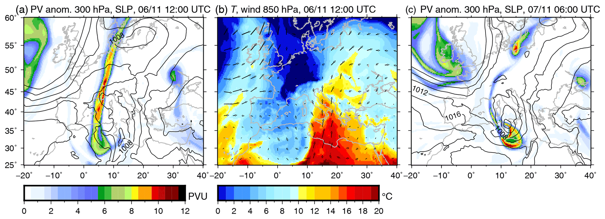
Figure 1Potential vorticity (PV) anomaly at 300 hPa (colour scale) and SLP (isocontours every 4 hPa) at 12:00 UTC on 6 November (a) and 06:00 UTC on 7 November (c); temperature (colour scale, ∘C) and wind at 850 hPa at 06:00 UTC on 6 November (b) from the ERA5 reanalysis.
2.2 Simulations
Three numerical simulations of the event were performed using the state-of-the-art atmospheric model Meso-NH (Lac et al., 2018) and the oceanic model NEMO (Madec and the NEMO Team, 2016).
2.2.1 Atmospheric model
The non-hydrostatic French research model Meso-NH version 5.3.0 is used here with a fourth-order centred advection scheme for the momentum components and the piecewise parabolic method advection scheme from Colella and Woodward (1984) for the other variables, associated with a leapfrog time scheme. A C grid in the Arakawa convention (Mesinger and Arakawa, 1976) is used for both horizontal and vertical discretisations, with a conformal projection system of horizontal coordinates. A fourth-order diffusion scheme is applied to the fluctuations of the wind variables, which are defined as the departures from the large-scale values. The turbulence scheme (Cuxart et al., 2000) is based on a 1.5-order closure coming from the system of second-order equations for the turbulent moments derived from Redelsperger and Sommeria (1986) in a one-dimensional simplified form assuming that the horizontal gradients and turbulent fluxes are much smaller than their vertical counterparts. The mixing length is parameterised according to Bougeault and Lacarrere (1989), who related it to the distance that a parcel with a given turbulent kinetic energy at level z can travel downwards or upwards before being stopped by buoyancy effects. Near the surface, these mixing lengths are modified according to Redelsperger et al. (2001) to match both the Monin–Obukhov similarity laws and the free-stream model constants. The radiative transfer is computed by solving long-wave and short-wave radiative transfer models separately using the ECMWF operational radiation code (Morcrette, 1991). The surface fluxes are computed within the SURFEX module (Surface Externalisée; Masson et al., 2013) using, over sea, the iterative bulk parameterisation ECUME (Belamari et al., 2005; Belamari and Pirani, 2007) linking the surface turbulent fluxes to the meteorological gradients through the appropriate transfer coefficients. The Meso-NH model shares its physical representation of parameters, including the surface flux parameterisation, with the French operational model AROME (Seity et al., 2011) used for the Météo-France NWP with a current horizontal grid spacing of 1.3 km. In this configuration, deep convection is explicitly represented, while shallow convection is parameterised using the eddy diffusivity Kain–Fritsch scheme (Pergaud et al., 2009).
In the present study, a first atmosphere-only simulation with a grid spacing of 4 km has been performed on a larger domain of 3200 km×2300 km (D1; see Fig. 2). This simulation started at 18:00 UTC on 6 November and lasted 42 h until 12:00 UTC on 8 November. Its initial and boundary conditions come from the ECMWF operational analyses Cy40R1 (horizontal resolution close to 16 km, 137 vertical levels) every 6 h.
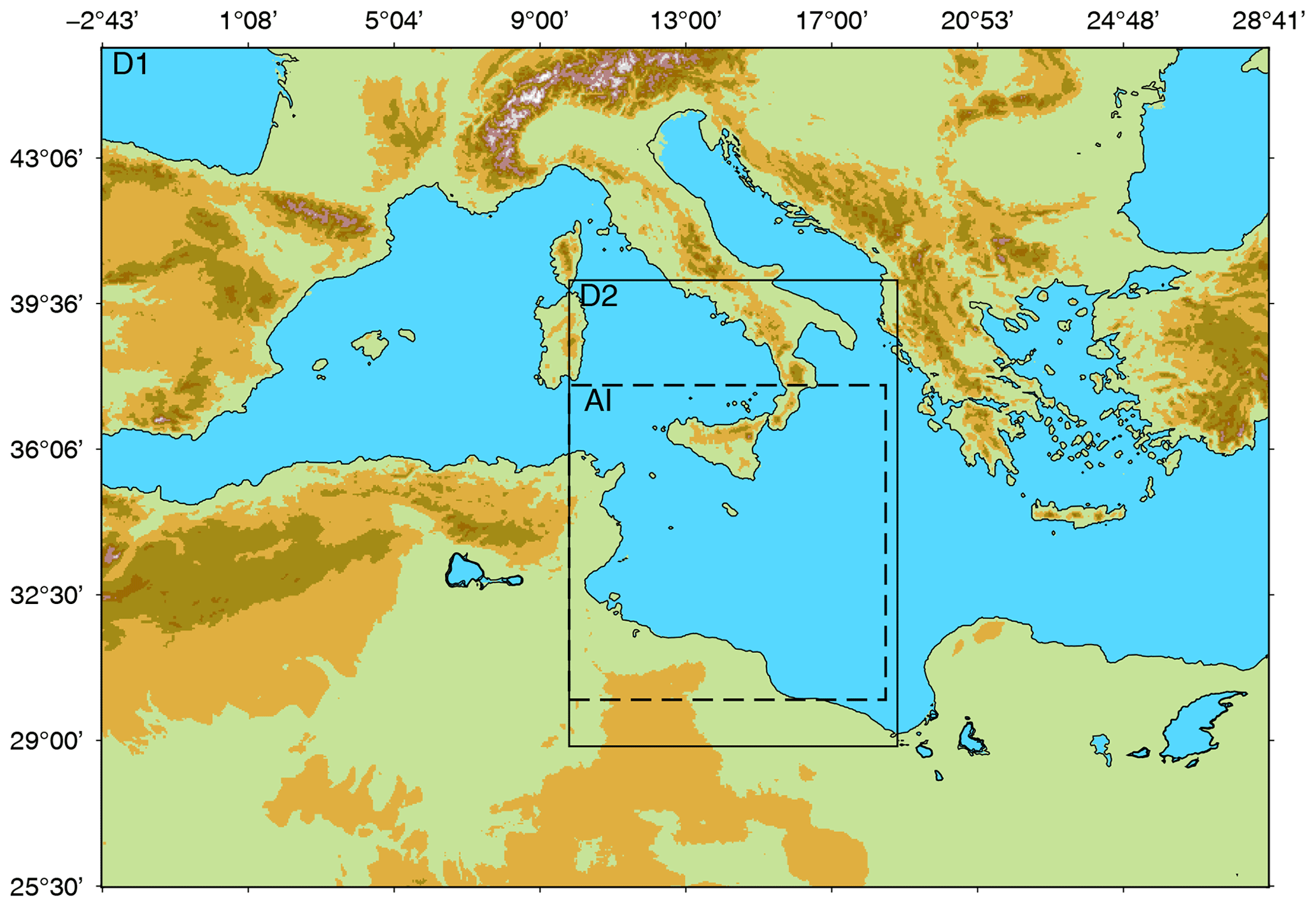
Figure 2Map of the large-scale domain D1, with the domain D2 indicated by the solid-line frame and the area of interest (AI) indicated by the dashed-line frame.
As described in the following, this 4 km simulation provides initial and boundary conditions for simulations on a smaller domain of 900 km×1280 km (D2; Fig. 2). This domain extension was chosen as a trade-off between computing time and an extension large enough to represent the physical processes involved in the cyclone life cycle, including the influence of the coasts. All simulations on the inner domain D2 share a time step of 3 s and their grid (with horizontal grid resolution of 1.33 km and 55 stretched terrain-following levels). Atmospheric and surface parameter fields are issued every 30 min.
2.2.2 Oceanic model
The ocean model used is NEMO (version 3_6) (Madec and the NEMO Team, 2016), with physical parameterisations as follows. The total variance dissipation scheme is used for tracer advection in order to conserve energy and enstrophy (Barnier et al., 2006). The vertical diffusion follows the standard turbulent kinetic-energy formulation of NEMO (Blanke and Delecluse, 1993). In the case of unstable conditions, a higher diffusivity coefficient of 10 m2 s−1 is applied (Lazar et al., 1999). The sea-surface height is a prognostic variable solved thanks to the filtered free-surface scheme of Roullet and Madec (2000). A no-slip lateral boundary condition is applied, and the bottom friction is parameterised by a quadratic function with a coefficient depending on the 2-D mean tidal energy (Lyard et al., 2006; Beuvier et al., 2012). The diffusion is applied along iso-neutral surfaces for the tracers using a Laplacian operator with the horizontal eddy diffusivity value νh of 30 m2 s−1. For the dynamics, a bi-Laplacian operator is used with the horizontal viscosity coefficient ηh of m4 s−1.
The configuration used here is sub-regional and eddy-resolving, with a 1∕36∘ horizontal resolution over an ORCA grid from 2.2 to 2.6 km resolution named SICIL36 (ORCA is a tripolar grid with variable resolution; Madec and Imbard, 1996), which was extracted from the MED36 configuration domain (Arsouze et al., 2013) and shares the same physical parameterisations with its “sister” configuration WMED36 (Lebeaupin Brossier et al., 2014; Rainaud et al., 2017). It uses 50 stretched z levels in the vertical, with level thickness ranging from 1 m near the surface to 400 m at the sea bottom (i.e. around 4000 m depth) and a partial step representation of the bottom topography (Barnier et al., 2006). It has four open boundaries corresponding to those of the D2 domain shown in Fig. 2, and its time step is set to 300 s. The initial and open boundary conditions come from the global 1∕12∘ resolution PSY2V4R4 daily analyses from Mercator Océan International (Lellouche et al., 2013).
2.2.3 Configuration of simulations
The 3-hourly outputs of the large-scale simulation on D1 are used as boundary and initial conditions for three different simulations on the smaller domain D2, based on the previously described atmospheric and oceanic configurations. These three simulations start at 00:00 UTC on 7 November and last 36 h, until 12:00 UTC on 8 November. The first atmosphere-only simulation called NOCPL uses a fixed SST forcing, while the CPL and NOCUR simulations are two-way coupled between Meso-NH and NEMO-SICIL36. In CPL, the SURFEX–OASIS coupling interface (Voldoire et al., 2017) enables exchanging the SST and two-dimensional surface currents from NEMO to Meso-NH and the two components of the momentum flux, the solar and non-solar heat fluxes and the freshwater flux from Meso-NH to NEMO every 15 min. The NOCUR run is similar, except that the surface currents are not transmitted from NEMO to Meso-NH.

Figure 3Comparison of the simulated tracks (triangles) of the non-coupled run (NOCPL; red), coupled run with SST only (NOCUR; cyan) and fully coupled run (CPL; blue) with the best track (black closed circles) based on observations as in Cioni et al. (2018). The position is shown every hour, with time labels every 3 h, starting at 09:00 UTC on 7 November until 12:00 UTC on 8 November. In colours is initial sea surface temperature (SST; ∘C) at 01:00 UTC on 7 November.
In order to ensure that the impact of the coupling in the NOCUR and CPL configurations originates from the time evolution of the SST rather than from a change in the initial SST field, the SST field used as a surface forcing in NOCPL is produced by the CPL run, 1 h after the beginning of the simulation (i.e. after the initial adjustment of the oceanic model). This field (Fig. 3) is kept constant throughout the simulation.
2.3 Validation
Figure 3 compares the tracks of Qendresa obtained in the three different simulations with the best track based on observations (brightness temperature from radiance in the 10.8 µm channel measured by the SEVIRI instrument aboard the MSG – Meteosat Second Generation – satellite; see Cioni et al., 2018). All the simulated tracks are shifted northwards with respect to the observations since the beginning of the simulations. The mean distance between the simulated and observed tracks is close to 85 km, with no significant difference between the simulations. Cioni et al. (2018) showed that using horizontal resolutions finer than 2.5 km is mandatory to accurately represent the fine-scale structure of this cyclone and its time evolution. Sensitivity studies showed that better resolution results in simulated track closer to observations. The best agreement is obtained with a nested configuration and an inner domain at 300 m resolution. In the present study, several sensitivity tests were performed on the smaller domain to improve the simulated track: (i) the starting time of the simulation was changed between 12:00 UTC on 6 November and 00:00 UTC on 7 November with an increment of 3 h; (ii) the number of vertical levels in Meso-NH was increased to 100, with stretching to ensure a better sampling in the atmospheric boundary layer; and (iii) the atmospheric simulation was performed without nesting, initial and boundary conditions from ECMWF, and a horizontal resolution of 2 km. Note that our inner domain D2 is close in its extension to the domain used by Cioni et al. (2018). None of these tests (eight in total) significantly improved the track, the northward shifting of the cyclone occurring in every case in the early hours of 7 November.

Figure 4Time series of the maximum of the 10 m wind speed and of the 10 m wind averaged over a 100 km radius around the cyclone centre (a) and minimum sea-level pressure (b) as obtained in the different simulations on 7 November and 8 November until 12:00 UTC. The thin red line in (a) indicates the 18 m s−1 wind speed threshold. The background shading (here and in the following time-series plots) indicates the development (light blue), mature (orange) and decay (grey) phases. The observations of SLP in Linosa (black plain circles) are shown for comparison in (b); the observations of wind speed from Malta, Lampedusa and Pantelleria are shown in (a) – see text.
The deepening and maximum intensity of the simulated cyclone are nevertheless close to the observed ones, even if a direct (i.e. co-localised) comparison is not possible due to the northward shift of its track. A strong deepening of almost 15 hPa is obtained in the first 12 h of the CPL simulation (Fig. 4b), with a minimum value at 12:30 UTC on 7 November close to the minimum observed at Linosa station. This station is the closest point to the best track at the time of the observed maximum intensity of the storm. The surface wind speed peaks at the same time (Fig. 4a), and its time evolution agrees well with METAR observations at the stations of Lampedusa, Pantelleria or Malta. Also, the time evolution of the wind speed averaged over a 50 km radius around the cyclone centre is in good agreement with the control simulation of Cioni et al. (2018). Despite the northward shift of its track, the medicane simulated by Meso-NH is very realistic and can be used to explore the processes at play, especially concerning the role of the sea surface thanks to the CPL simulation.
This part presents first the successive phases of the event based on an analysis of upper-level and mid-troposphere processes. Then, we assess the impact of accounting for the short-term evolution of the SST in the atmospheric surface processes.
3.1 Chronology of the simulated event
We use the methodology of Fita and Flaounas (2018) based on upper-level and low-level dynamics, asymmetry, and thermal wind to characterise the phases of the medicane. Figure 5 shows the 300 hPa PV anomaly, SLP, surface wind and equivalent potential temperature θe at 850 hPa from the NOCPL simulation. Phase space diagrams are commonly used to describe in a synthetic way the symmetric characteristics of the cyclone as well as the thermal characteristics and extent of its core. The present version in Fig. 6 showing the evolution of Qendresa from 01:00 UTC on 7 November to 12:00 UTC on 8 November is derived from the original work of Hart (2003) using the adaptation of Picornell et al. (2014) for smaller-scale cyclones. The radius used for computing the low-troposphere thickness asymmetry B and the low-troposphere and upper-troposphere thermal winds (−VTL and −VTU, respectively) were fitted to the radius of maximum wind at 850 hPa and is close to 100 km, and the low troposphere and upper troposphere are defined here as the 925–700 and 700–400 hPa levels, respectively. The radius value of 100 km is in agreement with several other studies focusing on medicanes and avoids a smooth-out of the warm-core structure (Chaboureau et al., 2012; Miglietta et al., 2011; Cavicchia et al., 2014; Picornell et al., 2014) but may lead to an underestimation of the cyclone extension. Indeed, the radius of maximum wind is ill defined or larger during the first stage of the cyclone, but it is steady and close to 90 km during the major part of its lifetime. As a result, the diagram obtained is likely less representative of the cyclone structure during its first hours but fits well after 10:00 UTC.
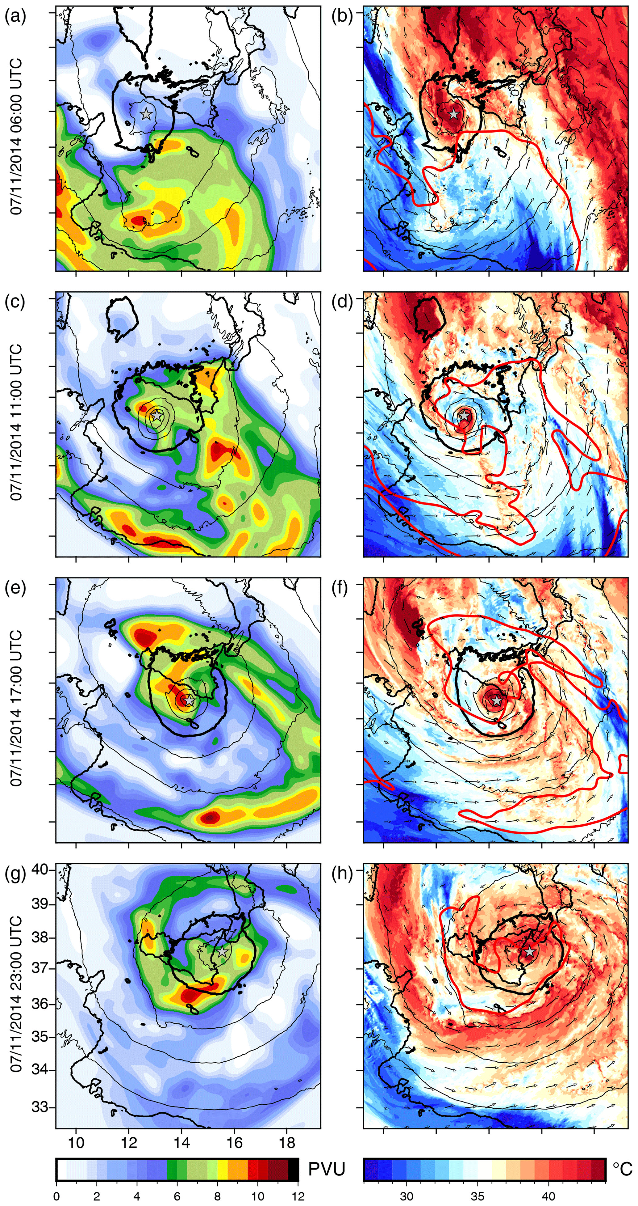
Figure 5Potential vorticity at 300 hPa (colour scale) and SLP (isocontours every 4 hPa; the 1000 hPa isobar is in bold) (a, c, e, g) and equivalent potential temperature (∘C; colour scale) and wind at 850 hPa, SLP, and 6 PVU at 300 hPa isocontours (red) (b, d, f, h) from the NOCPL simulation.
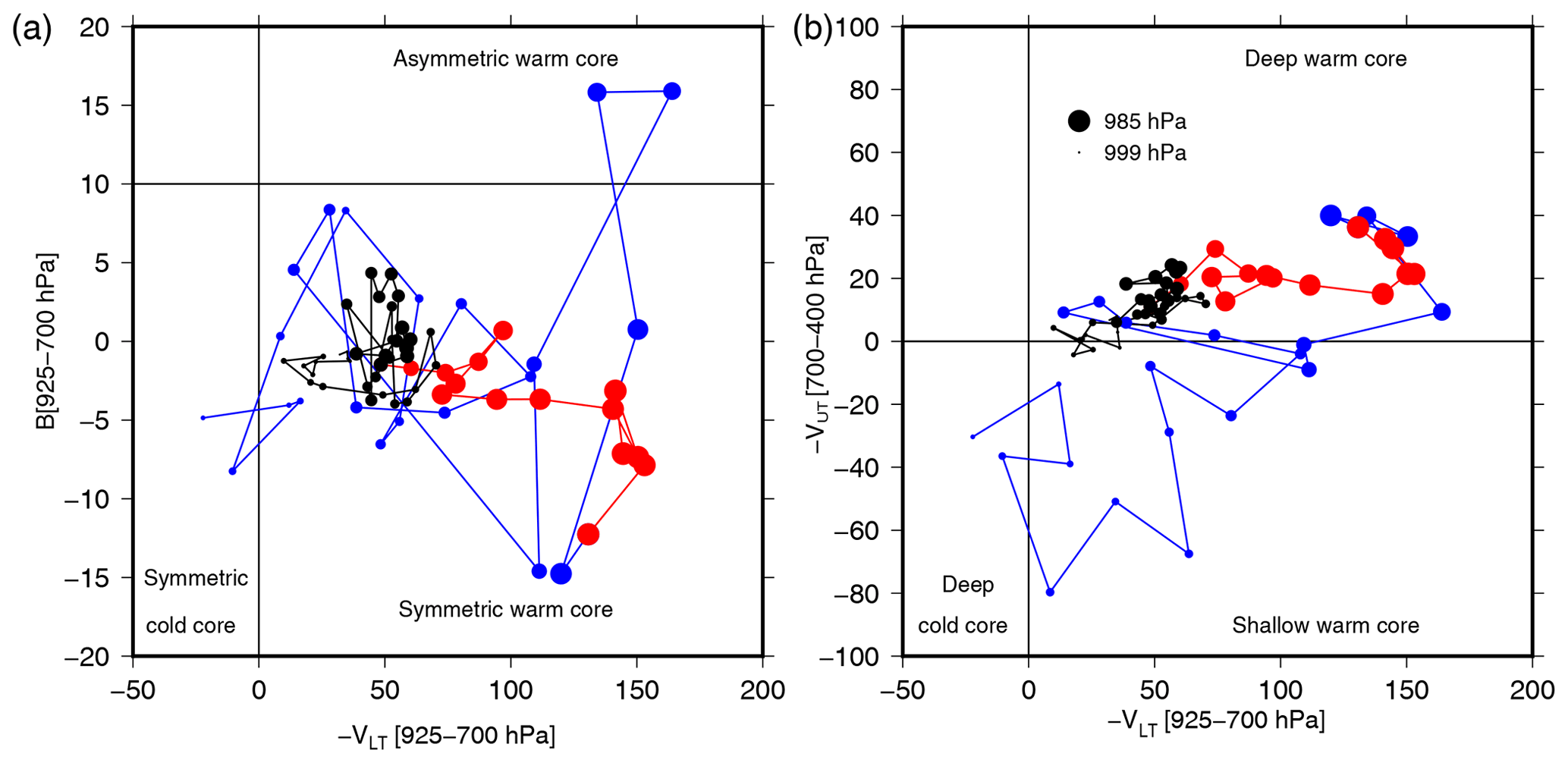
Figure 6Phase diagram of the NOCPL-simulated cyclone from 01:00 UTC on 7 November to 12:00 UTC on 8 November, with low-tropospheric thickness asymmetry inside the cyclone (B) with respect to low-tropospheric thermal wind (−VLT) (a) and upper-tropospheric thermal wind (−VUT) with respect to low-tropospheric thermal wind (b). The development phase is in blue, the mature phase in red and the decay phase in black.
At 06:00 UTC on 7 November, the PV streamer has moved northwards from Libya and is located to the south of the SLP minimum (Fig. 5a). A south–north cold front is visible in the 850 hPa θe, east of the cyclone centre, and the medicane centre is located under the left exit of the upper-level jet (Fig. 5b). The minimum SLP starts to decrease until reaching 985 hPa at around 11:00 UTC, corresponding to a strong deepening rate of 1.4 hPa h−1 for 10 h. This phase also marks the increase in the maximum wind at the low level and in the wind speed averaged over a 100 km radius around the cyclone centre (Fig. 4). It is referred to as “development phase” in the following. The heaviest rainfall occurs here (Fig. 7), with 10 h accumulated rain above 200 mm locally and instantaneous values above 50 mm h−1 east of Sicily and at sea between Pantelleria and Malta. As in Fita and Flaounas (2018), the maximum thermal wind is obtained during this phase (Fig. 6).
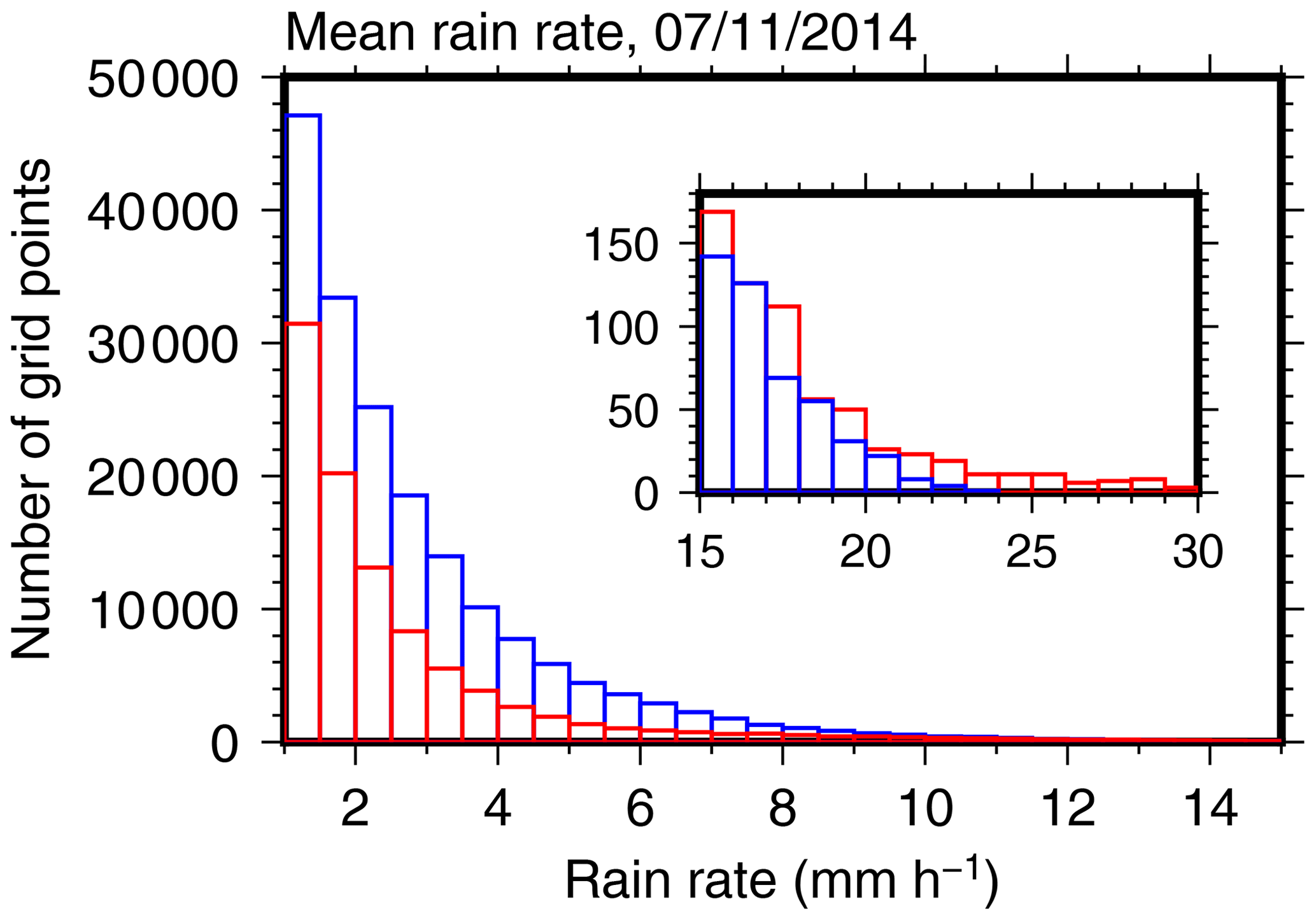
Figure 7Histogram of the mean rain rate distribution (in number of grid points) for the development (blue) and mature (red) phases in the NOCPL simulation. The enclosed figure zooms in on the highest rates.
Then, the upper-level jet moves further over the Ionian Sea and Sicily. The SLP minimum is aligned with the 300 hPa PV anomaly at 11:00 UTC on 7 November (Fig. 5c). This marks the beginning of the “mature phase”, with a maximum intensity at around 12:00 UTC (Fig. 4). The medicane presents the circular shape typical of tropical cyclones with spiral rainbands, and a warm, symmetric core (Fig. 5d) extended up to 400 hPa (Fig. 6). The upper-level PV anomaly stays wrapped around the SLP until 17:00 UTC, and both structures drift eastwards to the south of Italy (Fig. 5e). The medicane slowly decreases in intensity (Fig. 4) until it makes landfall in the southeast of Sicily at 18:00 UTC. The cold front drifts eastwards away of the cyclone centre, evolving into an occluded front wrapped around the SLP minimum (Fig. 5f). This mature phase, although the most intense of the cyclone, produces more scattered rainfall than the development phase (Fig. 7).
The cyclone then moves northeastwards towards the Ionian Sea and continuously weakens until 12:00 UTC on 8 November (“decay phase” hereafter). The SLP minimum steadily increases (Fig. 4); at this point, the upper-level PV anomaly has evolved into a cut-off and is still aligned with the cyclone centre (Fig. 5g), and the 850 hPa warm core has extended ∼250 km around the cyclone centre (Fig. 5h).
In the following, the impact of the ocean–atmosphere coupling on the cyclone intensity is assessed by comparing the results of the CPL, NOCUR and NOCPL simulations. The time period for this comparison is 7 November only, as the medicane lost a large part of its intensity in the evening of 7 November.
3.2 SST evolution
Taking into account the effect of the SST change only (NOCUR) results in a slightly slower and weaker deepening by 1.5 hPa and a maximum wind speed that is 3 m s−1 higher (Fig. 4). Including the effect of the surface currents on the atmospheric boundary layer gives a slightly more intense cyclone (1.5 hPa less and 8 m s−1 stronger maximum wind). Figure 3 shows no significant difference in the tracks between the NOCPL, NOCUR and CPL simulations, except when the cyclone centre loops east of Sicily at the end of the day. The median values of the SST difference between CPL and NOCPL over the whole domain and the values of the 5 %, 25 %, 75 % and 95 % quantiles are shown in Fig. 8. The median surface cooling is very weak (0.1 ∘C at the end of the development phase, ∼0.2 ∘C at the beginning of the decay phase). Its evolution during the decay phase is also weak, with values of 0.25 ∘C at 23:00 UTC, on 7 November. The maximum cooling is 0.6 ∘C. To focus on the effects of this surface cooling on the surface processes feeding the cyclone, we used a conditional sampling technique to isolate the areas with enthalpy flux above 600 W m−2 (this corresponds to the mean value of the 80 % quantile of the enthalpy flux on the day of 7 November). The enthalpy flux is defined here as the sum of the latent heat flux LE and the sensible heat flux H. In this area (EF600 hereafter), the SST difference and its time evolution are slightly larger, with a median difference of −0.2 ∘C at the beginning of the mature phase and −0.4 ∘C at the end of 7 November. In NOCUR, the SST difference in EF600 is slightly larger than in CPL, but the difference is not significant. The SST cooling in this area of less than 0.4 ∘C (median value) is much weaker than typical cooling values observed under tropical cyclones, which commonly reach 3 to 4 ∘C (e.g. Black and Dickey, 2008). In addition, the spatial extent of the cooling does not form a wake as in tropical cyclones (not shown).
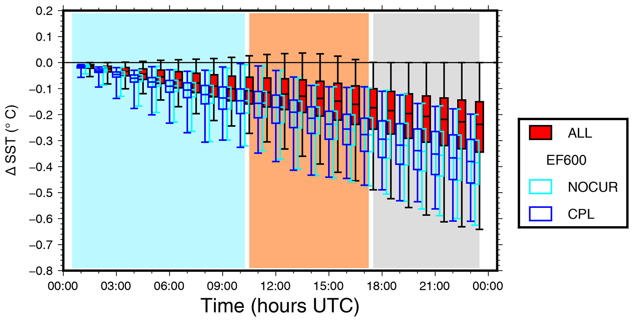
Figure 8Time series of the median differences between the SST in the CPL and NOCPL simulations, in the whole domain (red) and in the EF600 area (blue; see text for definition), on 7 November. The boxes indicate the 25 % and 75 % quantiles and the whiskers the 5 % and 95 % quantiles. The SST differences in the EF600 area between the NOCUR and NOCPL simulations are also shown (cyan). Some of the boxes have been slightly shifted horizontally for clarity.
The conclusion of this part is that surface cooling is 1 order of magnitude smaller than what is obtained under tropical cyclone, with no significant impact of the surface currents. However, quantifying the surface cooling in other medicanes could lead to contrasting results. For instance, a surface cooling of 2 ∘C was obtained in an ocean–atmosphere–waves coupled simulation of a strong storm in the Gulf of Lion (Renault et al., 2012). Investigating the reasons of such a discrepancy are beyond the scope of the present work. The stronger cooling could be due to the storm track staying at the same place in the Gulf of Lion for a long time. The difference can also come from a different oceanic preconditioning (their case occurred in May), with stronger stratification or a shallower mixed layer that amplifies cooling due to the mixing and entrainment process.
3.3 Impact on turbulent surface exchanges
A comparison of the time evolution of the turbulent fluxes in the NOCPL and CPL simulations shows very weak differences even in the EF600 area (Fig. 9a). At the end of the run, the mean difference of the enthalpy flux is 25 W m−2, with a standard deviation of 13 W m−2. This is weak compared to the values of the turbulent fluxes on this area, between 500 and 800 W m−2 for LE and 100 and 250 W m−2 for H. Expressed in percentage of the fluxes, the relative difference is ∼2 % at the beginning of the mature phase and 5 % at 21:00 UTC on 7 November. The difference of H is 7±4 W m−2 (relative difference between 4 % and 10 %). Thus, coupling has a very weak impact on the turbulent heat fluxes even in the EF600 area. Again, the effect of the surface currents (CPL vs. NOCUR in Fig. 9b) is not significant.
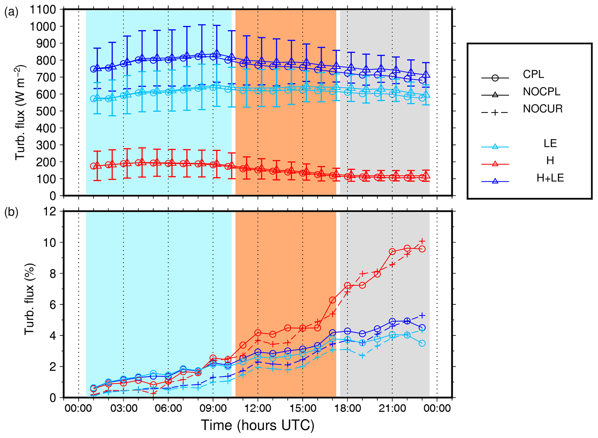
Figure 9Time series of the mean values and standard deviations (error bars) of the total turbulent heat flux (blue), latent heat flux (cyan) and sensible heat flux (red) in the CPL (open circles) and NOCPL (triangles) simulations (a) and of the mean difference between CPL and NOCPL turbulent fluxes (open circles; same colour code) and between NOCUR and NOCPL turbulent fluxes, in percentage relative to the NOCPL values (b) in the EF600 area.
In the following, except if otherwise specified, the results of the NOCPL simulation are used to investigate the medicane behaviour, focusing on the area of interest (AI in Fig. 2).
This section investigates which surface parameters control the surface heat fluxes during the different phases of the medicane, among the SST, surface wind, temperature and humidity.
4.1 Representation of surface fluxes and methods
In numerical atmospheric models, the turbulent heat fluxes are classically computed as a function of surface parameters using bulk formulae:
Here, ρ is the air density, cp the air thermal capacity and Lv the vaporisation heat constant. The gradient ΔU corresponds to the wind speed at the first level with respect to the sea surface, Δθ is the difference between the SST and the potential temperature at the first level θ, and Δq is the difference between the specific humidity at saturation, with temperature equal to SST and the specific humidity at the first level. The transfer coefficients Ch and Ce are defined as
and
with κ being the von Karman's constant, ψT and ψq empirical functions describing the stability dependence, Chn and Cen the neutral transfer coefficient for heat and moisture, and L the Obukhov length (which depends, in turn, on the virtual potential temperature at the first level and on the friction velocity u∗). In the ECUME parameterisation used in this study, the neutral transfer coefficients Chn and Cen are defined as polynomial functions of the 10 m equivalent neutral wind speed (defined as in Geernaert and Katsaros, 1986). They also depend on the wind speed at 10 m and on the Obukhov length through the stability functions. The Obukhov length is expressed as in Liu et al. (1979):
with Tv being the virtual temperature at the first level, depending on the temperature and specific humidity, and Tv∗ the scale parameter for virtual temperature, depending on the temperature and humidity at the first level. As a consequence, the transfer coefficients depend as the fluxes on the wind speed, on the temperature and specific humidity at the first level, and on the SST. In the following, we do not distinguish between the temperature and potential temperature at the first level.
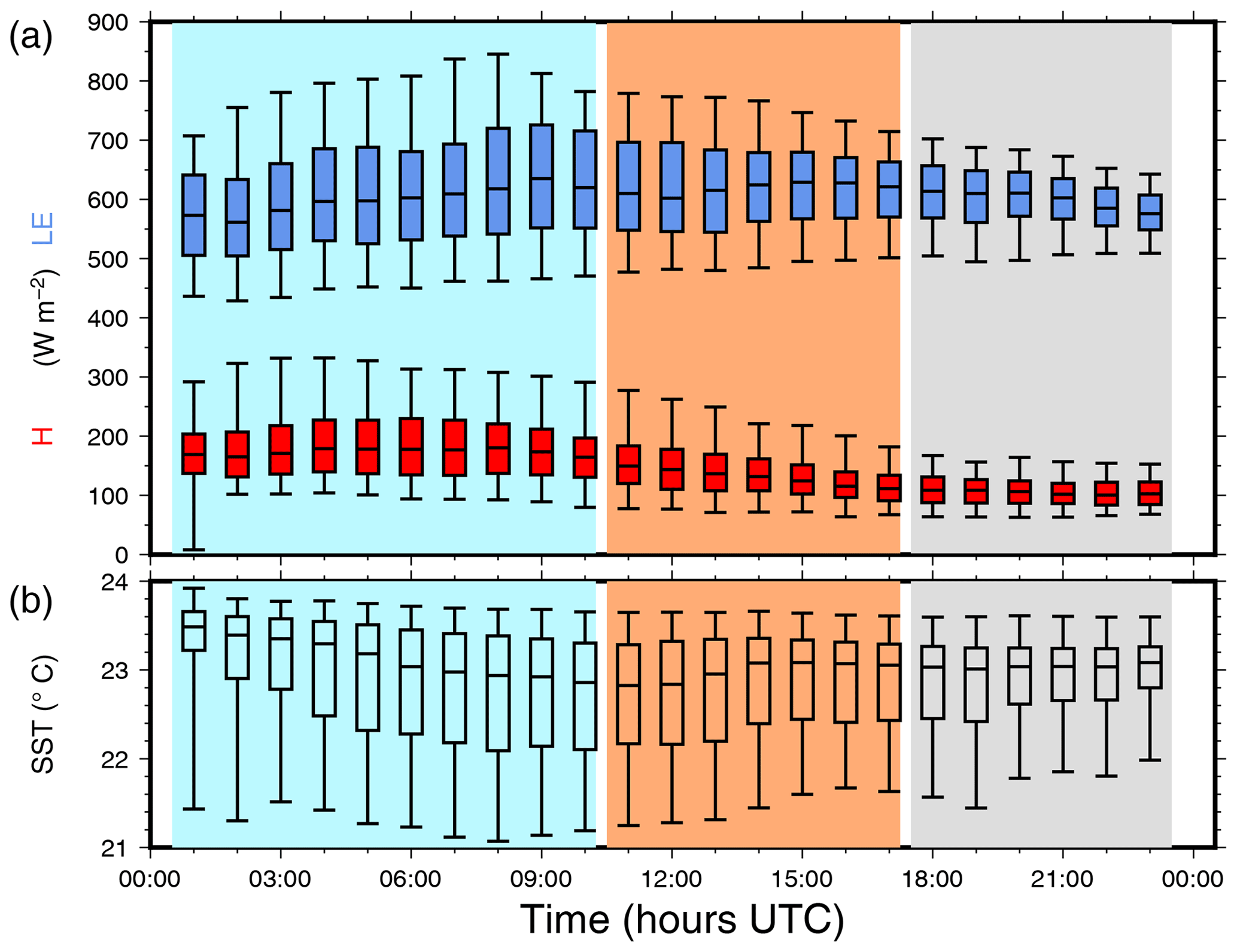
Figure 10Time series of the median values of latent (blue) and sensible heat fluxes (red; a) and of SST (b) in the EF600 area (see text) in the NOCPL run on 7 November. The boxes corresponds to the 25 % and 75 % quantiles and the whiskers to the 5 % and 95 % quantiles.
The time evolution of the median values and 5 %, 25 %, 75 % and 95 % quantiles of the latent and sensible heat fluxes is given in Fig. 10a for 7 November, in the EF600 area, and the time evolution of the median values and quantiles of the SST in Fig. 10b. The latent heat flux is always much higher than the sensible heat flux, as this is generally the case at sea when the SST is above 15 ∘C (e.g. Reale and Atlas, 2001). The sensible heat flux represents here 22 % of the enthalpy flux during the development phase and 12 % to 15 % during the decay phase. Both fluxes have asymmetric distributions, with upper tails (95 %) longer than lower tails (5 %). This is partly due to the conditional sampling ( W m−2) used here, as low fluxes are cut off. The median value of H is maximum at the end of the development phase (180 W m−2 at 08:00 UTC), while its 95 % quantile is maximum at the beginning of the development phase (332 W m−2 at 04:00 UTC). During the mature phase, both the median and 95 % quantile values of H decrease continuously. Conversely, the median value of LE is maximum (635 W m−2) at 09:00 UTC during the development phase, and it stays approximately constant until 15:00 UTC. The 95 % quantile is maximum (845 W m−2) at the end of the development phase. LE starts to decrease later and more slowly than H (at around 15:00 UTC, as the system has started to weaken). The median values of LE in this EF600 sampling are constant or slightly increasing until the evening (20:00 UTC), whereas the minimum values (5 % quantile) increase continuously until the end of the day. Again, this is probably partly due to the sampling used here.
The distributions of the SST are asymmetric throughout the event, with lower tails much longer than upper tails (Fig. 10b). The SST maximum (close to 24 ∘C) is almost constant with time. The lower and median values vary due to the conditional sampling EF600 and the motion of the cyclone away from the warm SST area.
To investigate the mutual dependencies and co-variabilities of the fluxes and parameters listed above, we used the rank correlation of Spearman, which corresponds to the linear correlation between the rank of the two variables in their respective sampling (Myers et al., 2010). This metric enables relating the variables of interest monotonically rather than linearly and is more appropriate in the case of non-linear relationships.
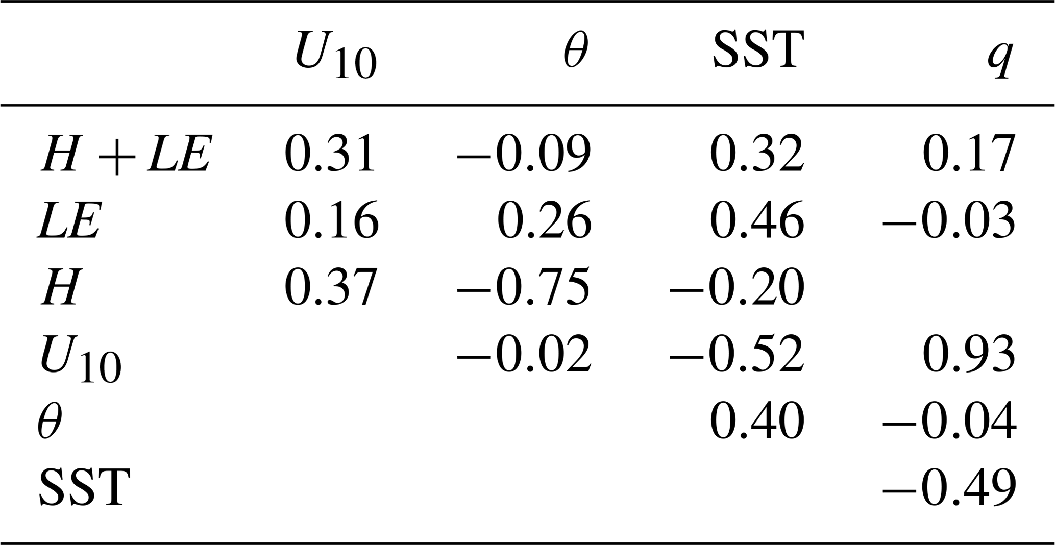
The co-variabilities are analysed in the whole domain first, to determine the main contribution to the fluxes globally, then in the EF600 area to isolate surface processes controlling the growth and maturity of the medicane. The values are given in Tables 1 to 3 for the EF600 area and for three time periods of the development, mature and decay phases, respectively, i.e. 09:00, 13:00 and 18:00 UTC on 7 November.
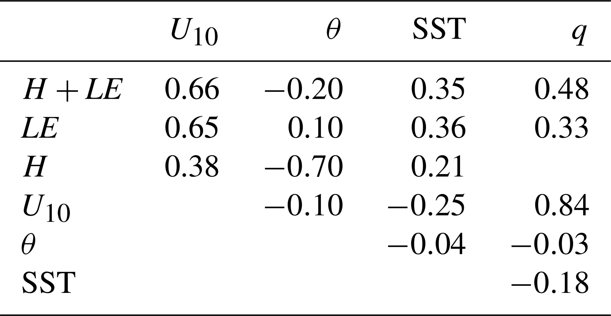
Table 1Spearman's rank correlations between the enthalpy flux, latent and sensible heat flux, and related parameters (10 m wind speed U10, potential temperature at 10 m θ, SST and humidity at 10 m q) at 09:00 UTC on 7 November, from the CPL simulation, in the EF600 area.

4.2 Development phase
At the low level, this phase corresponds to a low-pressure system resulting from the evolution of the instability generated by the lee cyclone of the northern African relief, with strong baroclinic structures. During the first hours, the areas of heavy precipitation are co-localised with frontal structures. A warm sector is visible east of the domain, with a cold front extending southeast from the south of Italy and a very strong low-level convergence between the southeasterly flow in the warm sector and the south-to-southwesterly flow in the cold sector (see Fig. 5b).
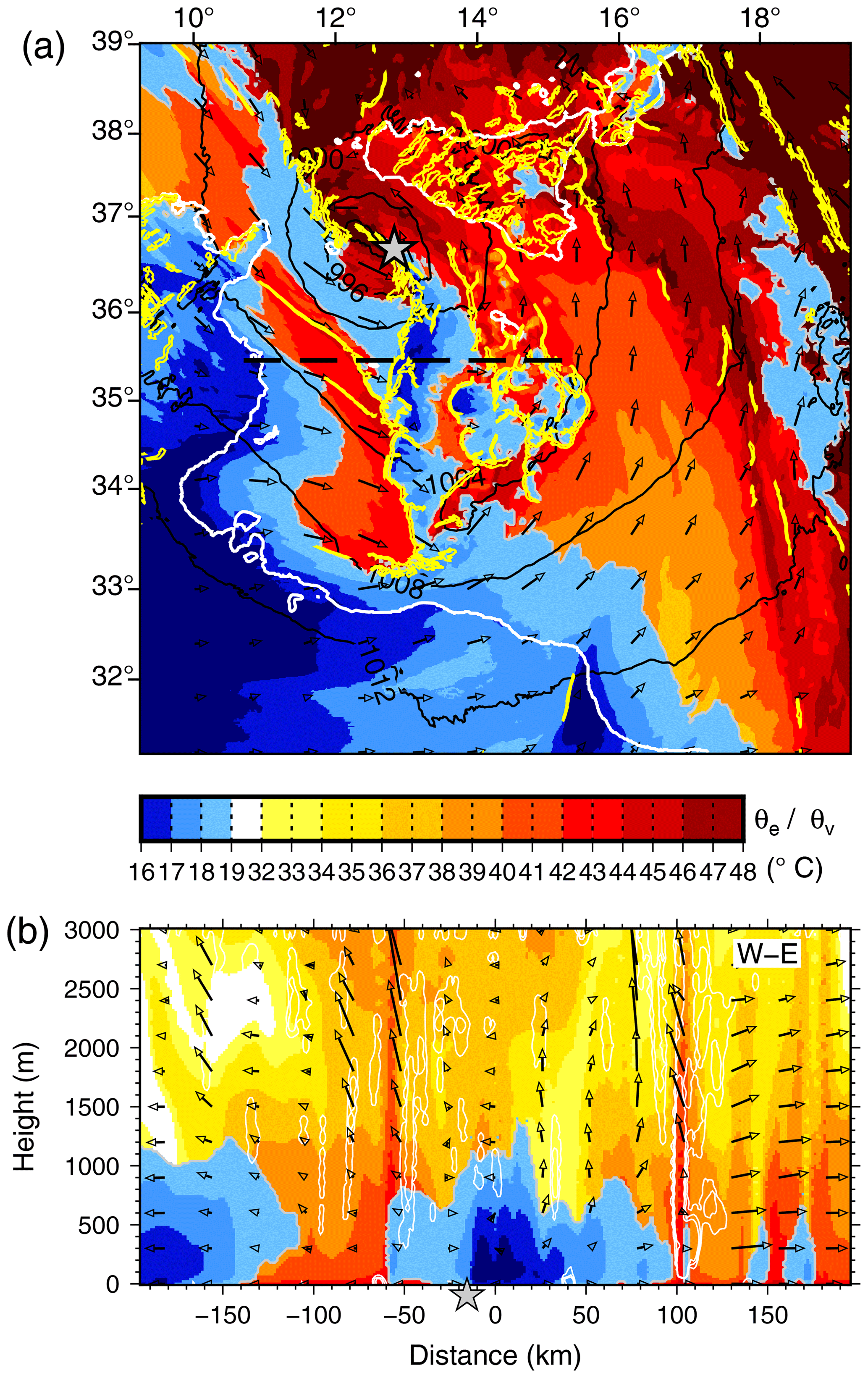
Figure 11Map of equivalent potential temperature (warm colours) and virtual potential temperature below 19 ∘C (blue shades) at first level; horizontal convergence rate above m s−2 at 100 m (yellow contours), 10 m wind (arrows) and SLP (black contours) at 08:30 UTC on 7 November (a); and vertical cross section of equivalent potential temperature and virtual potential temperature (colour scale), tangential wind (black vectors; the vertical component is amplified by a factor 20), and potential vorticity anomaly (white contour at 5 PVU) along a west–east transect (b) (dashed line in a). Grey stars indicate the position of the SLP minimum.
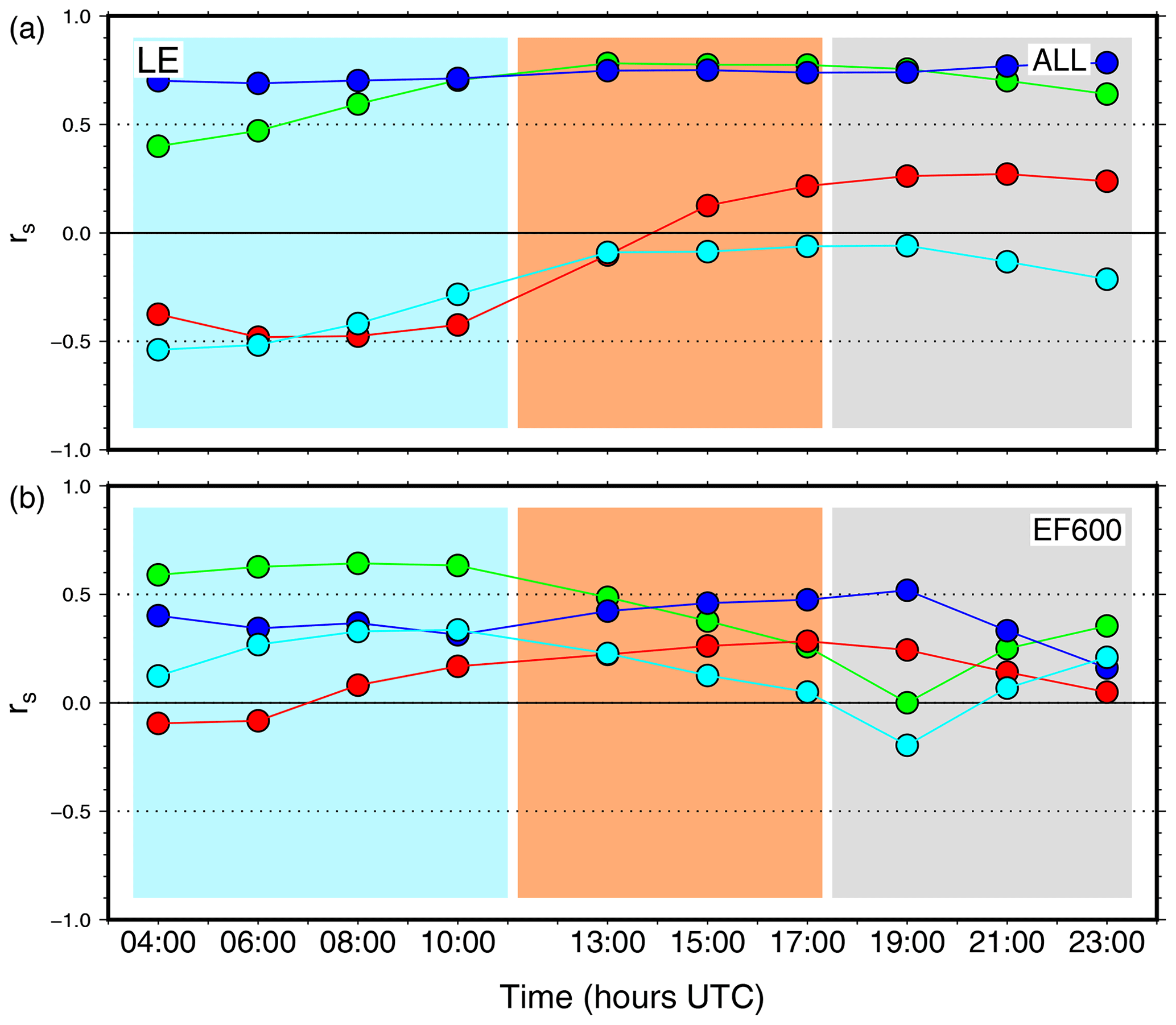
Figure 12Time series of Spearman's rank-order correlation rs between the latent heat flux LE and 10 m wind speed (green), potential temperature at 10 m (red), SST (blue), and specific humidity at 2 m (cyan) in the whole domain (a) and in the EF600 area (b) in the CPL simulation.
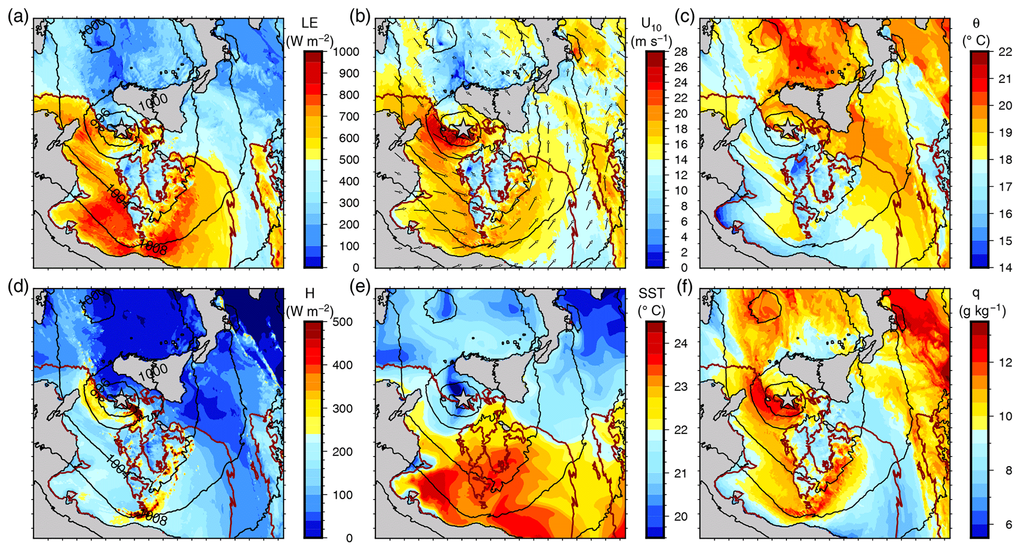
Figure 13Maps of the turbulent heat fluxes LE (a), H (d), 10 m wind U10 (b), 10 m potential temperature (c), SST (e) and specific humidity at 2 m (f) at 09:00 UTC on 7 November in the CPL simulation.
At 08:30 UTC on 7 November (Fig. 11), strong convergence lines develop close to the cyclonic centre, between Sicily and Tunisia. The low-level virtual potential temperature θv superimposed onto the equivalent potential temperature θe is used here as a marker of cold pools (with an upper limit of 19 ∘C for θv – Ducrocq et al., 2008; Bresson et al., 2012). Some of these cold pools result from evaporation under convective precipitation, while those located at sea along the northern African coast originate from dry and cold air advected from inland. The discrimination between these two kinds of cold pools was done using a simulation without the latent heat transfer due to rain evaporation (not shown here). The cold and moist air spreads to the surface, following density currents, and is advected northeastwards by the low-level flow. To the west and south of the domain, cold pools were formed at night by radiative processes over land and were advected over sea with a vertical extent of ∼1000 m (see the westernmost part of the W–E transect; Fig. 11b).
The upwind edge of the cold pools is the place of strong horizontal convergence at the low level, leading to uplift and deep convection of air masses with high θe. During the development phase, the cold pools move northwards with the southerly flow, towards the centre of the cyclone. Then, they contribute to triggering convection in the northwesterly low-level flow with high θe (Fig. 11b). The warm surface anomaly propagates close to the cyclone centre (now located under the 300 hPa PV anomaly) up to 3000 m and generates a low- to mid-troposphere PV anomaly. At the same time, a dry-air intrusion from the upper levels brings air masses with low θe and relative humidity below 20 % to 3000 m, resulting in an upper-to-mid-troposphere PV anomaly (Fig. 15a and c).
To identify the surface parameters controlling evaporation at sea, the time evolution of the Spearman's rank correlations between LE, U10, θ, the SST and q is given in Fig. 12 and Tables 1 to 3.
During this phase, in the whole domain, the parameters governing LE are the SST and the wind (positively correlated), the specific humidity (negatively) and the potential temperature (negatively). Potential temperature and humidity are also strongly positively correlated (rs=0.55 over the whole domain) because cold and dry air is advected from the Tunisian and Libyan continental surface by the southerly low-level flow (Fig. 13b, c and f; at 09:00 UTC). This air mass progressively charges itself in heat and moisture in the area of strongest enthalpy fluxes at sea to the north of Libya (Fig. 13a). The EF600 area, with strong fluxes and cold and dry air, corresponds also to warm SSTs (Fig. 13e). Here, LE is mainly controlled by the wind and by the SST, θ has no effect (weak or negative correlations; Fig. 12b, Table 1) and q has a weak effect.
LE is always much higher than H (Fig. 10a), resulting in the “strong flux area” EF600 being controlled by LE rather than H. LE is also more homogeneous than H in EF600. However, H can be strong locally (Fig. 13d). During this development phase, H is controlled mainly by θ at the first level (Fig. 14), partly indirectly through the stratification and transfer coefficient (not shown). In the EF600 area also, H is mainly governed by θ ( at 09:00 UTC), the SST influence is always weak and the wind plays a secondary role. The enhanced control by the potential temperature is partly due to the continental air masses advected from northern Africa and partly to the presence of the cold pools under the areas of deep convection and strong wind.
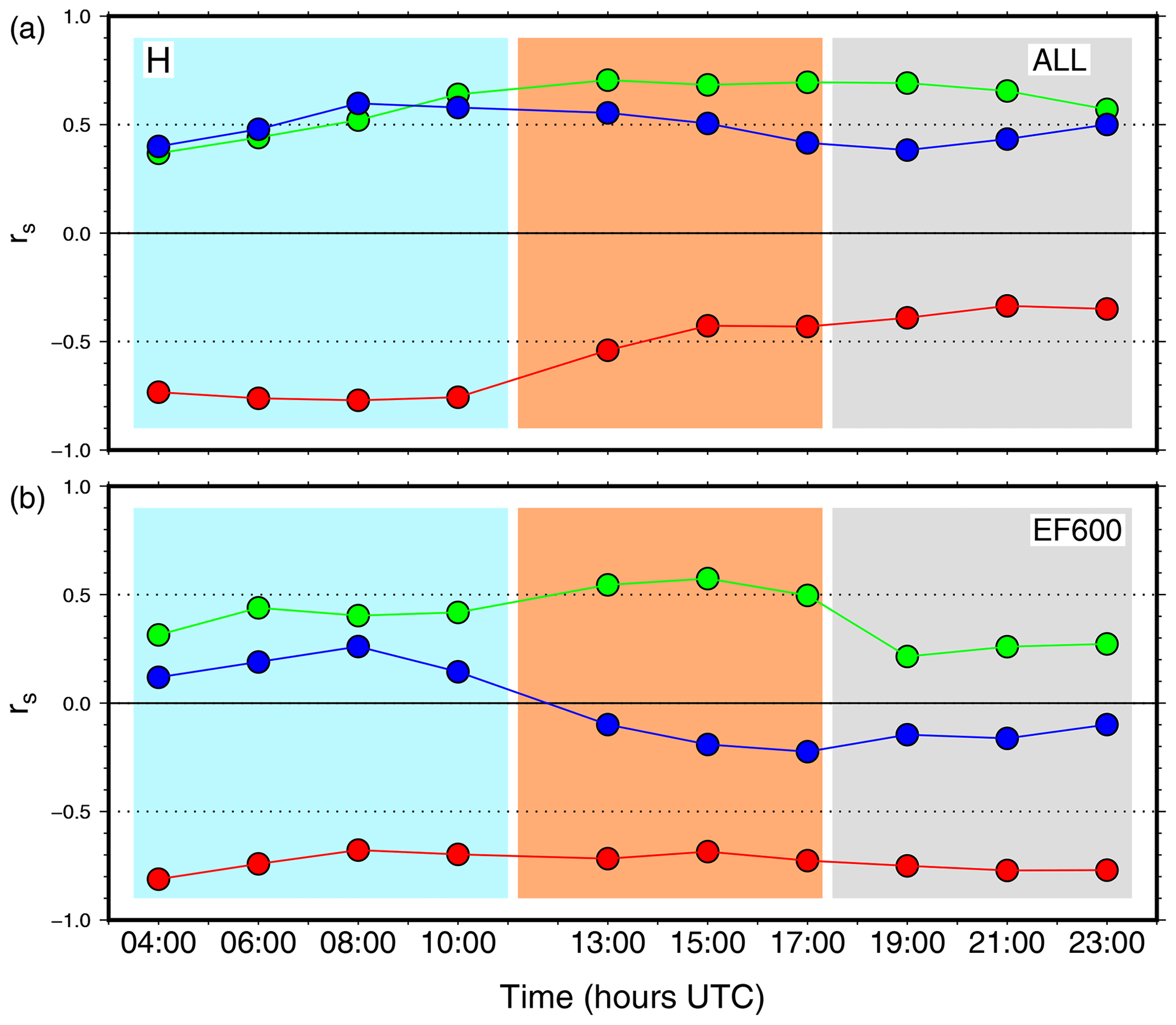
Figure 14Same as Fig. 12 but between the sensible heat flux H and 10 m wind speed (green), potential temperature at 10 m (red), and SST (blue).
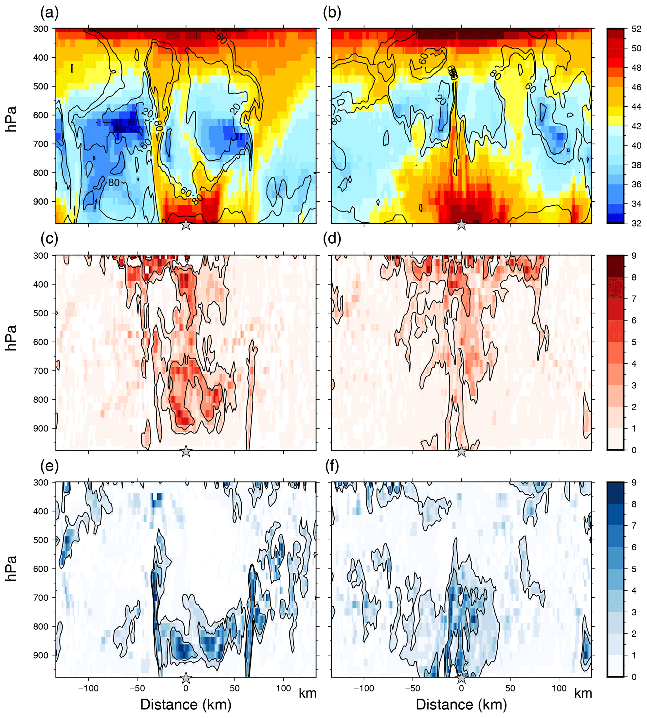
Figure 15Vertical cross sections of equivalent potential temperature θe (∘C; colour scale) and relative humidity (%; isolines) (a, b), DPV (intensity) (c, d), and WPV (intensity) (e, f) on a west–east transect across the cyclone centre, at 13:00 (a, c, e) and 18:00 UTC (b, d, f) on 7 November, in the CPL simulation. The black contours in (c) to (f) correspond to intensities 1 and 3 (as defined in Miglietta et al., 2017).
4.3 Mature phase
At 13:00 on 7 November, the PV anomalies at 700 and 300 hPa are aligned (Fig. 15c, e). A zonal cross section on the SLP minimum shows that a low-level PV anomaly above 5 PVU formed around the cyclone centre, extending from the surface up to the 300 hPa anomaly (Fig. 15). The warm core extends up to 850 hPa (Fig. 15a). Its upward development is limited by colder air (low θe) brought from aloft. There is low-level convergence (up to 800 hPa) towards the cyclone centre, and deep convection close to the centre, but no or very weak divergence at the mid-troposphere to upper troposphere. The cyclonic circulation was reinforced with horizontal wind speed above 8 m s−1 at every level more than 10 km away from the cyclone centre.
During this phase and the previous one, over the whole domain as in the EF600 area, evaporation is controlled equivalently by the SST and the wind speed, with a decreasing influence of the humidity (Fig. 12, Table 2). The EF600 area extends further north, closer to the cyclone centre, away from the area of cold and dry low-level air. This cold-air inflow starts to warm and moisten under the combined impact of the diurnal warming of the continental surfaces (not shown) and of the strong enthalpy fluxes offshore (Fig. 16a, c and f). The sensible heat flux is still controlled by the temperature, with an increasing influence of the wind (Table 2).

Figure 16Same as Fig. 13 but at 13:00 UTC on 7 November.
4.4 Decay phase
In the afternoon of 7 November, the cyclone first moves towards colder SSTs in the east of the Strait of Sicily (Fig. 3). Then, it crosses Sicily and reaches the Ionian Sea with even colder SSTs at around 20:00 UTC before slowly decaying and losing its tropical characteristics. Back trajectories are used to check whether warm- and moist-air extraction from the sea surface contributes to high θe values obtained around the cyclone centre. They are based on the method of Schär and Wernli (1993), adapted by Gheusi and Stein (2005). The chosen trajectories originate from three different places and arrive at the same place, at three vertical levels surrounding the level closest to 1500 m, at 23:00 UTC on 7 November (Fig. 17). Their equivalent potential temperature ranges from 31 to 38 ∘C at their first appearance in the domain and is close to 45 ∘C on average at their final point. Of these trajectories, θe increases almost continuously, with a strong jump during their transit at the low level (below 500 m) above the sea in the EF600 area (white contour in Fig. 17). A separate analysis of the two different stages in the trajectories was performed. Stage 1 corresponds to the period when the particles remain in the low-level flow (between 200 and 1200 m a.s.l.) south and east of Sicily and stage 2 to their convective ascent from ∼300 to 1500 m. During stage 1, the potential temperature of the particles decreases by 1 ∘C on average, while the mixing ratio increases by 2.8 g kg−1. This shows that the increase in θe is due to strong surface evaporation. During stage 2, the mixed ratio of the particles decreases by 2 g kg−1, and their potential temperature increases by 4.1 ∘C. This indicates condensation and latent heating and demonstrates the strong role of the sea surface in increasing the moisture and heat of the low-level flow before its approach on the cyclone centre and of diabatic processes in reinforcing its warm core.
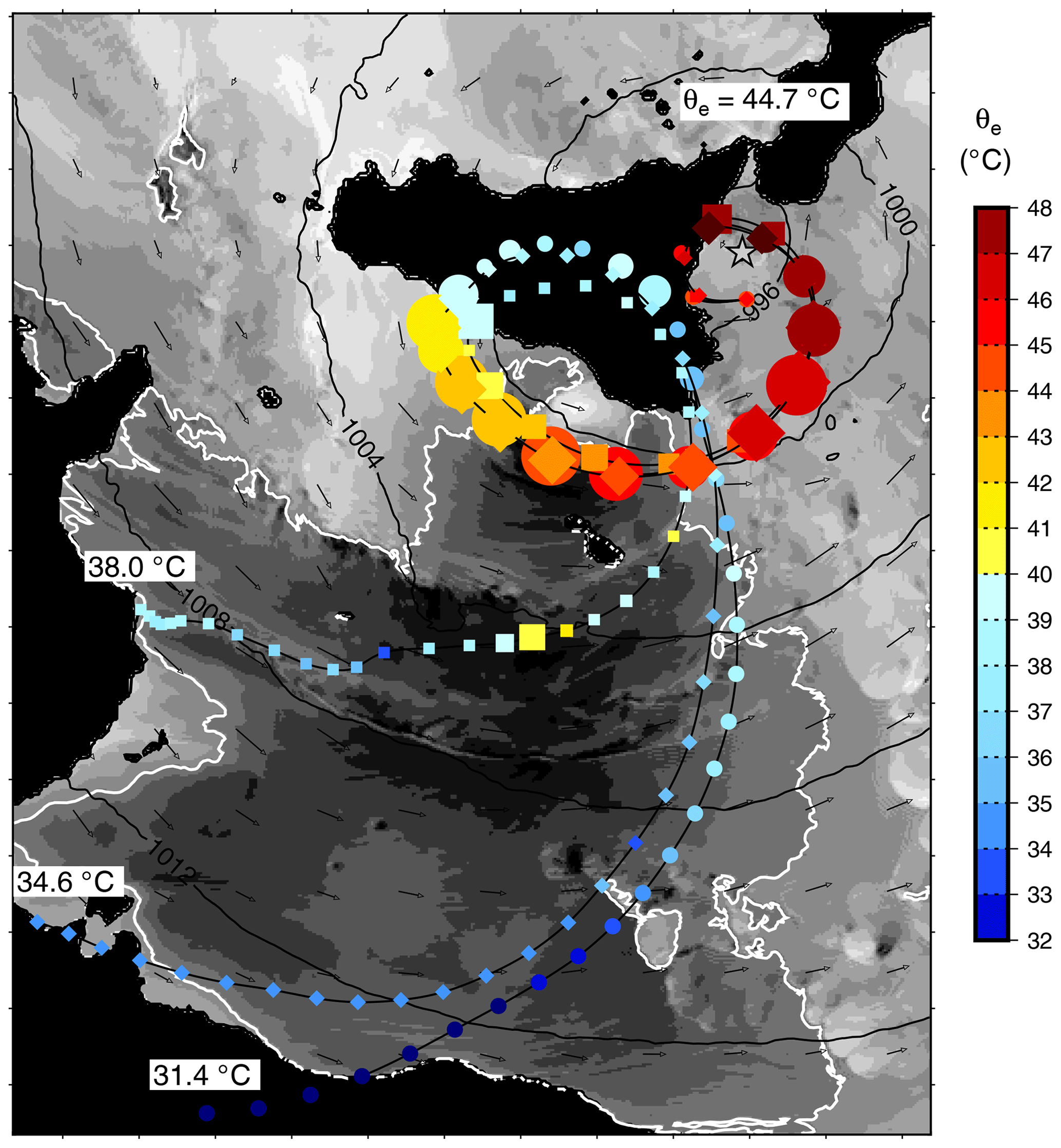
Figure 17Map of the back trajectories of air parcels arriving south of the cyclone centre at 23:00 UTC on 7 November, 1500 m a.s.l., at three different levels (circles, squares and diamonds). The first point of the trajectories corresponds to the start of the D2 domain simulation (00:00 UTC on 7 November). The colour scale indicates the equivalent potential temperature (∘C), and the size of the symbol is inversely proportional to altitude between 0 and 1000 m and constant above 1000 m. Also shown are the values of the final equivalent potential temperature and of the initial equivalent potential temperatures, the wind field at 900 hPa (black vectors), and the surface enthalpy flux (grey shades) with a threshold at 600 W m−2 (white contour) at 15:30 UTC, when the particles arrive at sea to the south of Sicily.
During the decay phase and in the whole domain the influence of the humidity on LE is weak (Fig. 12a). EF600 is still located on warm SSTs south of the domain (Fig. 18a, e) and corresponds also to the strongest winds on the right-hand side of the cyclone (Fig. 18b). Within this area, there is almost no influence of the temperature or humidity on LE (Table 3). The influence of the wind speed is decreasing; the role of the SST is strong until 21:00 UTC. After that, the cyclone reaches the northern Ionian Sea with much colder SSTs, and the effect of the wind speed becomes dominant at the very end (Fig. 12b). The sensible heat flux is governed by the wind (see the strong N–S gradient in Fig. 18b) rather than by the low-level temperature, except in the northern part of EF600 (where the wind speed is also the highest).
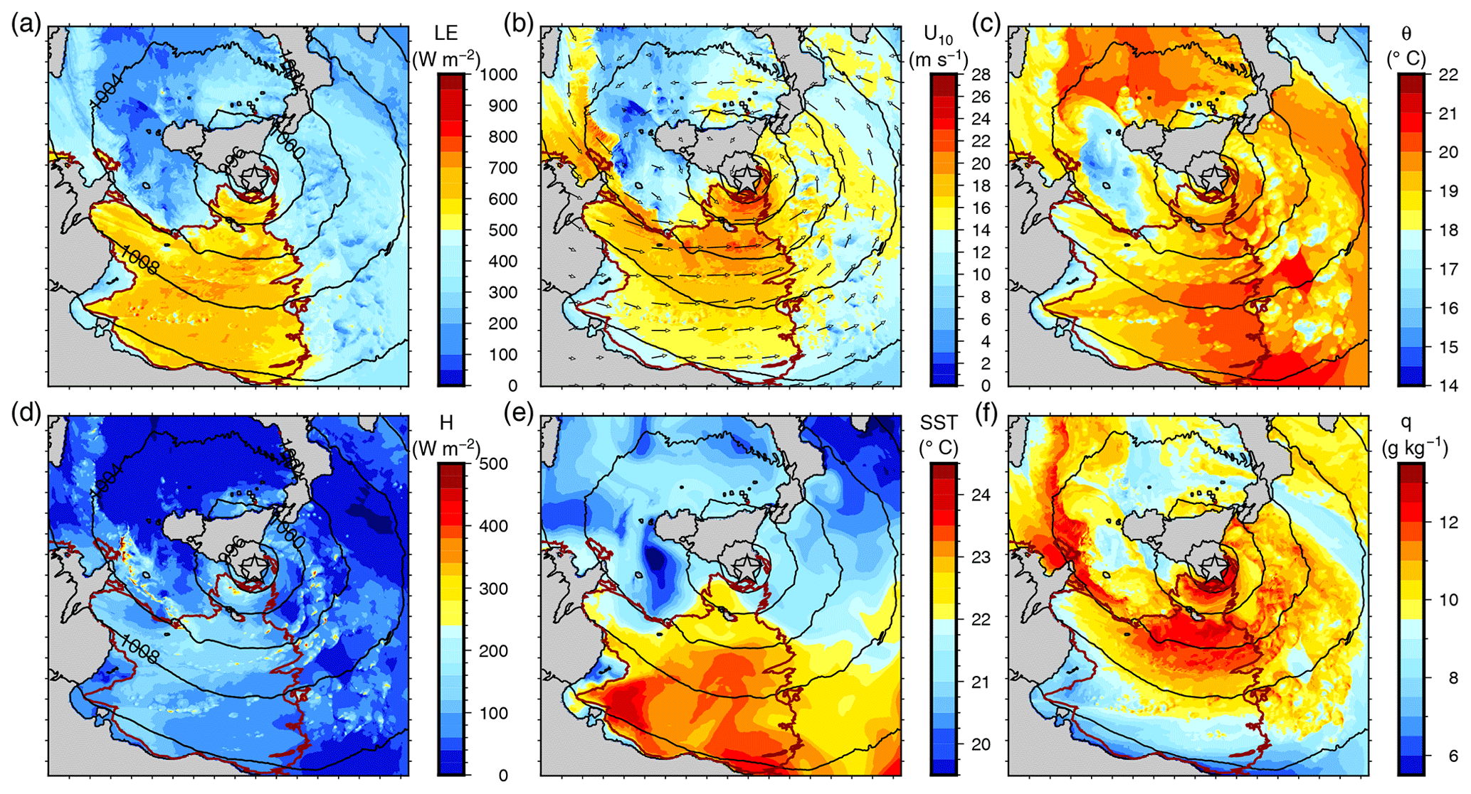
Figure 18Same as Fig. 13 but at 18:00 UTC on 7 November.
In summary, at the scale of the domain, both strong winds (in the cold sector during the development phase, then close to the cyclone centre and on its right side) and warm SSTs (in the south of the domain) are necessary for strong latent heat fluxes. Within the area of strong fluxes (also strong winds and warm SSTs), the evaporation is mainly controlled by the wind (development and mature phases) instead of by the SST (decay phase). In contrast, the sensible heat flux depends mainly on the potential temperature in the surface layer. Colder air masses lead to strong sensible heat flux rather than strong wind or warmer SSTs. During the two first phases, cold air is either advected from northern Africa or created by evaporation under convective precipitation (cold pools). During the decay phase, strong latent heat transfer over high SSTs warms the near-surface atmospheric layer and lowers the sensible heat transfer.
The comparison of the simulations with and without ocean coupling shows no significant impact of the evolution of the SST on the track, intensity or life cycle of the medicane. The weak SST cooling, notably during the first 24 h of the simulation, is likely responsible for that. In the strong flux area, where the enthalpy flux feeding the cyclone in heat and moisture maintains the convection and the latent heat release, the median value of the SST cooling is between 0.2 and 0.4 ∘C. The effect on H is −7 W m−2 during the mature phase and −12 W m−2 at 23:00 UTC on 7 November (less than 10 %). On LE, it is −19 and −37 W m−2 for the same two time periods (less than 5 %). Coupling with the surface currents has no significant impact on the simulation.
Nevertheless, in this specific case, the SST exerts a strong control on the latent heat flux that dominates the surface heat transfer throughout the event. During the development phase, there is also a strong influence of peculiarities of the central Mediterranean: the transition between deep convection and heavy precipitation associated with baroclinic processes and the cyclone taking place downwind of the dry and cold low-level flow from northern Africa. These air masses with low θv encounter moist and warm air at sea and enhance the deep convection, together with the cold pools formed by rain evaporation and downdrafts. These cold pools of various origins displace the deep convection at sea. Uplift of warm air masses increases the low-level PV and reinforces the vortex, which is moved northeastwards, closer to the PV anomaly aloft.
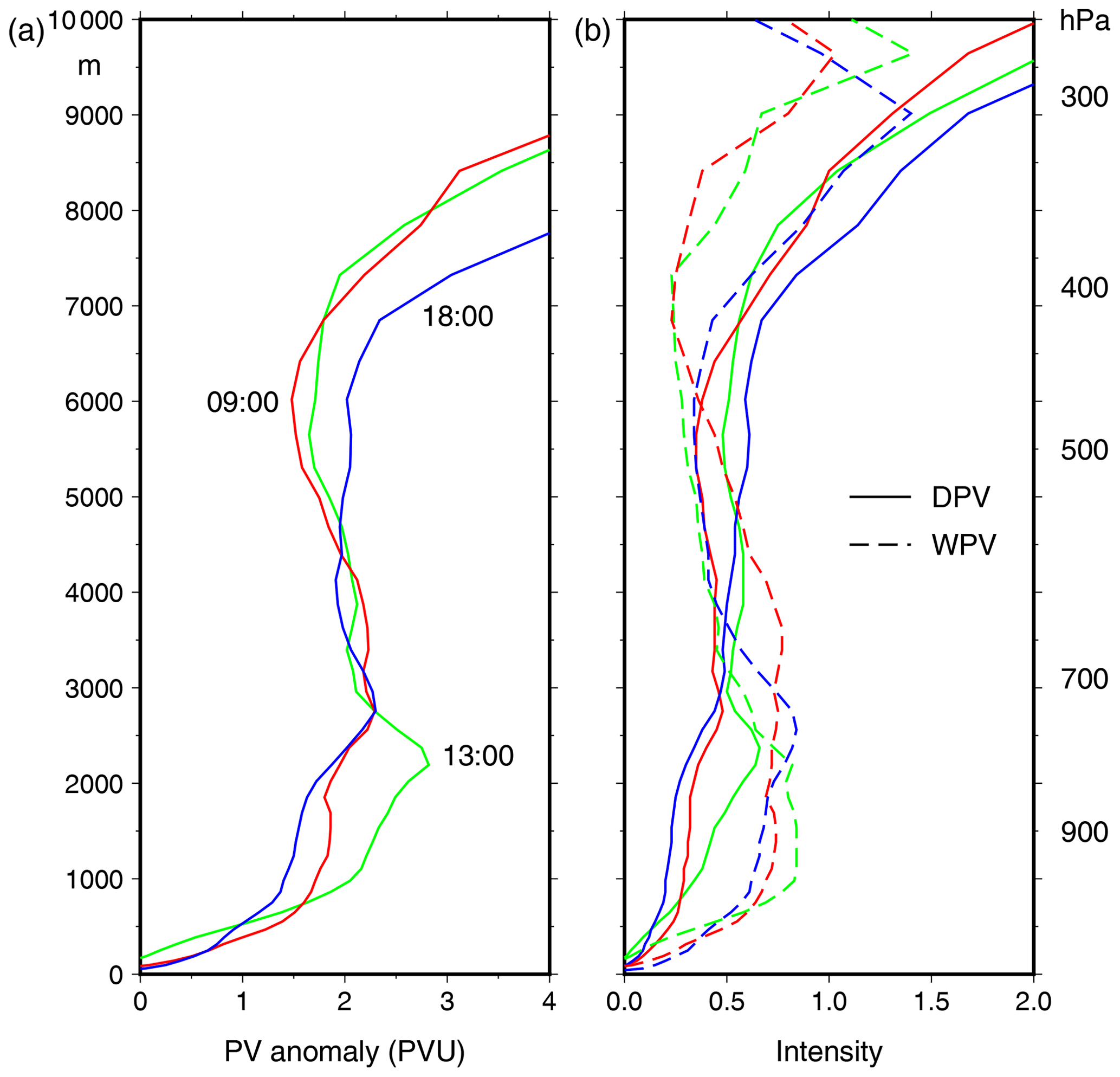
Figure 19Vertical profiles of PV (a) and DPV and WPV (b) averaged within a 100 km radius circle around the cyclone centre at 09:00 (red), 13:00 (green) and 18:00 UTC (blue) on 7 November in the CPL simulation.
Better knowing the intensity and the role of air–sea exchanges and the related mechanisms could permit sorting medicanes, as proposed by Miglietta and Rotunno (2019). Is the present case governed by WISHE-like mechanisms or rather by diabatic and baroclinic processes throughout its lifetime (second category in Miglietta and Rotunno, 2019)? Strong air–sea exchanges at the surface and latent heat release act to build the warm-core anomaly, as seen in Sects. 4.3 and 4.4. The surface enthalpy fluxes take intermediate values, with a maximum above 1500 W m−2 for a few hours in areas with warm SST and strong winds downwind of the dry low-level flow from northern Africa. Thermal features characteristic of tropical cyclones are present, like low-level cold-air advection from the south to the east and warm-air advection from the south to the north (Reale and Atlas, 2001). The gradient of θe between the surface and 900 hPa is around 6–7 ∘C. The wrapping of the PV streamer around the cyclone centre evolves into an upper-level cut-off at the end of the decay phase. Conversely, some typical features are not present: even if there is weak low-level convergence around the cyclone centre, no divergence is seen at the upper level. The maximum latent heat flux within the EF600 area is more controlled by the SST than by the wind speed (Figs. 12b and 13a, b and e). No minimum of potential temperature or potential vorticity develops at 300 hPa close to the cyclone centre during the mature phase, as a marker of the PV anomaly erosion by the convective activity, and the upper-level PV anomaly never completely detaches from the large-scale structure.
Figure 19 shows the vertical profiles of wet PV and dry PV (WPV and DPV; defined as in Miglietta et al., 2017) averaged on the 100 km radius circle around the cyclone centre. WPV is produced diabatically by latent heat release (their Eq. 4), and DPV is generated by intrusion of stratospheric air into the upper troposphere (their Eq. 3). The vertical profiles of PV, DPV and WPV show a minimum WPV between 700 and 400 hPa during the decay phase and a clear difference between DPV and WPV at the low level (Fig. 19b). The DPV is weak up to the mid-troposphere and increases sharply above 400 hPa. The WPV anomaly at the low level develops up to 700 hPa during the development phase, but its vertical extent reduces to 800 hPa during the mature phase (13:00 UTC – see also Fig. 15e). This is due to a dry-air intrusion during the mature and decay phases, which is limited downwards by the warm core (Fig. 15a). At the beginning of the decay phase, at 18:00 UTC, the latent heating within the cyclone core increases the low-level WPV and erodes the dry and cold (θe) air masses up to 650 hPa. The warm-core and WPV anomaly extend upwards (Fig. 15b, f), and the DPV anomaly is pushed up to 700 hPa (Fig. 15c, d).
This suggests that the medicane of November 2014 as simulated in this study presents characteristics close to an extratropical cyclone or medicane of the second category as in Miglietta and Rotunno (2019). Its development phase is triggered by a PV streamer bringing instability at the upper level and baroclinic processes followed by strong convection at sea. This convection is enhanced and maintained by cold pools due to rain evaporation at the low level or by advection of dry and cold air from northern Africa. The conjunction of advection of continental air masses with evaporation under storms has not been identified as leading to tropical transition of Mediterranean cyclones so far, even though it is probably rather ubiquitous. Indeed both phenomena are rather widespread in the Mediterranean. Surface fluxes are strong and contribute to enhancing the convection potential until the mature phase of the cyclone. Evaporation is mainly controlled by the SST and by the wind speed during the whole event, while the temperature difference between the SST and the cold air advected from northern Africa during the development and mature phase play a strong role during its development. The vertical development of the warm core is limited by a dry-air intrusion that does not reach the lowest levels of the troposphere. Dry-air intrusions have been recognised as common processes in Mediterranean cyclones by Flaounas et al. (2015), but their role in the cyclone life cycle was not clearly assessed. Here, we suggest that they can act to limit the extent of the convection at the beginning of the mature phase. The convective activity is stronger during the development than during the mature phase of the cyclone, resulting in heavy rainfall 12 to 6 h before the maximum wind speed, consistent with previous studies based on observations (Miglietta et al., 2013; Dafis et al., 2018). Finally, these results are consistent with those of Carrió et al. (2017), which show, by using a factor separation technique, that while the role of the upper-level PV anomaly is crucial in preconditioning the event, its rapid deepening is due to the synergy of latent heat release and upper-level dynamics.
Coupling the atmospheric model with a 3-D high-resolution oceanic model shows that, in the present case, the surface cooling is too weak to impact the atmospheric destabilisation processes at the low level. Nevertheless, the effect of the medicane on the oceanic surface layer is probably significant. To better understand the sea surface evolution and the role of coupling, the ocean mixed layer response to the medicane and the mechanisms involved will be investigated in more detail in future work.
The source codes are available online (WaveWatchIII at https://polar.ncep.noaa.gov/waves/wavewatch/, NOAA, 2020; OASIS at https://portal.enes.org/oasis, CERFACS, 2020; Meso-NH at http://mesonh.aero.obs-mip.fr/mesonh54, LA and CNRM, 2020, and SURFEX at http://www.umr-cnrm.fr/surfex/, CNRM, 2020).
The availability of additional data is indicated in the Sect. “Acknowledgements”.
MNB and CLB designed the simulations. MNB performed the simulations. Both authors interpreted the results and wrote the paper.
The authors declare that they have no conflict of interest.
This article is part of the special issue “Hydrological cycle in the Mediterranean (ACP/AMT/GMD/HESS/NHESS/OS inter-journal SI)”. It is not associated with a conference.
This work is a contribution to the HyMeX programme (Hydrological cycle in the Mediterranean eXperiment – http://www.hymex.org, last access: 8 June 2020) through INSU-MISTRALS support. The authors acknowledge the Pôle de Calcul et de Données Marines for the DATARMOR facilities (storage, data access, computational resources). The authors acknowledge the MISTRALS/HyMeX database teams (ESPRI/IPSL and SEDOO/OMP) for their help in accessing the surface weather station data. The PSY2V4R4 daily analyses were made available by the Copernicus Marine Environment Monitoring Service (http://marine.copernicus.eu, last access: 8 June 2020). The ERA5 reanalysis at hourly timescales (https://doi.org/10.24381/cds.bd0915c6) is produced by the European Centre for Medium-Range Weather Forecasts (ECMWF) and made available by the Copernicus Climate Change Service (https://cds.climate.copernicus.eu, last access: 8 June 2020). METAR observations of SLP and wind were retrieved through the Weather Underground portal at https://www.wunderground.com (last access: 8 June 2020). The authors thank Jean-Luc Redelsperger (LOPS) for valuable discussions. We also thank Emmanouil Flaounas and two anonymous reviewers, whose comments helped to greatly improve this paper.
This paper was edited by Christian Barthlott and reviewed by Emmanouil Flaounas and two anonymous referees.
Akhtar, N., Brauch, J., Dobler, A., Béranger, K., and Ahrens, B.: Medicanes in an oceanatmosphere coupled regional climate model, Nat. Hazards Earth Syst. Sci., 14, 2189–2201, https://doi.org/10.5194/nhess-14-2189-2014, 2014.
Arsouze, T., Beuvier, J., Béranger, K., Somot, S., Lebeaupin Brossier, C., Bourdallé-Badie, R., Sevault, F., and Drillet, Y.: Sensibility analysis of the Western Mediterranean Transition inferred by four companion simulations, The Mediterranean Science Commission, Monaco, in: Proceedings of the 40th CIESM Congress, November 2013, Marseille, France, 2013.
Barnier, B., Madec, G., Penduff, T., Molines, J.-M., Treguier, A.-M., Le Sommer, J., Beckmann, A., Biastoch, A., Böning, C., Dengg, J., Derval, C., Durand, E., Gulev, S., Remy, E., Talandier, C., Theetten, S., Maltrud, M., McClean, J., and De Cuevas, B.: Impact of partial steps and momentum advection schemes in a global ocean circulation model at eddy-permitting resolution, Ocean Dynam., 56, 543–567, https://doi.org/10.1007/s10236-006-0082-1, 2006.
Belamari, S.: Report on uncertainty estimates of an optimal bulk formulation for surface turbulent fluxes, Marine EnviRonment and Security for the European Area–Integrated Project (MERSEA IP), Deliverable D, 4, CNRM, Toulouse, 2005.
Belamari, S. and Pirani, A.: Validation of the optimal heat and momentum fluxes using the ORCA2-LIM global ocean-ice model, Marine EnviRonment and Security for the European Area–Integrated Project (MERSEA IP), Deliverable D, 4, CNRM, Toulouse, 2007.
Beuvier, J., Béranger, K., Lebeaupin Brossier, C., Somot, S., Sevault, F., Drillet, Y., Bourdallé-Badie, R., Ferry, N., and Lyard, F.: Spreading of the Western Mediterranean deep water after winter 2005: time scales and deep cyclone transport, J. Geophys. Res.-Oceans, 117, C07022, https://doi.org/10.1029/2011JC007679, 2012.
Black, W. J. and Dickey, T. D.: Observations and analyses of upper ocean responses to tropical storms and hurricanes in the vicinity of Bermuda, J. Geophys. Res., 113, C08009, https://doi.org/10.1029/2007JC004358, 2008.
Blanke, B. and Delecluse, P.: Variability of the tropical Atlantic Ocean simulated by a general circulation model with two different mixed-layer physics, J. Phys. Oceanogr., 23, 1363–1388, https://doi.org/10.1175/1520-0485(1993)023<1363:VOTTAO>2.0.CO;2, 1993.
Bougeault, P. and Lacarrère, P.: Parameterization of Orography-Induced Turbulence in a Mesobeta-Scale Model, Mon. Weather Rev., 117, 1872–1890. https://doi.org/10.1175/1520-0493(1989)117<1872:POOITI>2.0.CO;2, 1989.
Bresson, E., Ducrocq, V., Nuissier, O., Ricard, D., and de Saint-Aubin, C.: Idealized numerical study of southern France heavy precipitating events: Identification of favouring ingredients, Q. J. Roy. Meteor. Soc., 138, 1751–1763, 2012.
Carrió, D. S., Homar, V., Jansà, A., Romero, R., and Picornell, M. A.: Tropicalization process of the 7 November 2014 Mediterranean cyclone: numerical sensitivity study, Atmos. Res., 197, 300–312, 2017.
Cavicchia, L., von Storch, H., and Gualdi, S.: A long-term climatology of medicanes, Clim. Dynam., 43, 1183–1195, https://doi.org/10.1007/s00382-013-1893-7, 2014.
CERFACS: OASIS, available at: https://portal.enes.org/oasis, last access: 8 June 2020.
Chaboureau, J.-P., Pantillon, F., Lambert, D., Richard, E., and Claud, C.: Tropical transition of a Mediterranean storm by jet crossing, Q. J. Roy. Meteor. Soc., 138, 596–611, 2012.
Cioni, G., Cerrai, D., and Klocke, D.: Investigating the predictability of a Mediterranean tropical-like cyclone using a storm-resolving model, Q. J. Roy. Meteor. Soc., 144, 1598–1610, https://doi.org/10.1002/qj.3322, 2018.
Claud, C., Alhammoud, B., Funatsu, B. M., and Chaboureau, J.-P.: Mediterranean hurricanes: large-scale environment and convective and precipitating areas from satellite microwave observations, Nat. Hazards Earth Syst. Sci., 10, 2199–2213, https://doi.org/10.5194/nhess-10-2199-2010, 2010.
CNRM: SURFEX, available at: http://www.umr-cnrm.fr/surfex/, last access: 8 June 2020.
Colella, P. and Woodward, P. R.: The Piecewise Parabolic Method (PPM) for Gas-Dynamical Simulations, J. Comput. Phys., 54, 174–201, https://doi.org/10.1016/0021-9991(84)90143-8, 1984.
Cuxart, J., Bougeault, P., and Redelsperger, J. L.: A turbulence scheme allowing for mesoscale and large-eddy simulations, Q. J. Roy. Meteor. Soc., 126, 1–30, https://doi.org/10.1002/qj.49712656202, 2000.
D'Asaro, E. A., Sanford, T. B., Niiler, P. P., and Terrill, E. J.: Cold wake of Hurricane Frances, Geophys. Res. Lett., 34, L15609, https://doi.org/10.1029/2007GL030160, 2007.
Dafis, S., Rysman, J. F., Claud, C., and Flaounas, E.: Remote sensing of deep convection within a tropical-like cyclone over the Mediterranean Sea, Atmos. Sci. Lett., 19, e823, https://doi.org/10.1002/asl.823, 2018.
Davolio, S., Miglietta, M. M., Moscatello, A., Pacifico, F., Buzzi, A., and Rotunno, R.: Numerical forecast and analysis of a tropical-like cyclone in the Ionian Sea, Nat. Hazards Earth Syst. Sci., 9, 551–562, https://doi.org/10.5194/nhess-9-551-2009, 2009.
Di Muzio, E., Riemer, M., Fink, A. H., and Maier-Gerber, M.: Assessing the predictability of Medicanes in ECMWF ensemble forecasts using an object-based approach, Q. J. Roy. Meteor. Soc., 145, 1202–1217, 2019.
Ducrocq, V., Nuissier, O., and Ricard, D.: A numerical study of three catastrophic precipitating events over southern France. Part II: Mesoscale triggering and stationarity factors, Q. J. Roy. Meteor. Soc., 134, 131–145, https://doi.org/10.1002/qj.199, 2008.
Emanuel, K. A.: An air–sea interaction theory for tropical cyclones. Part I: Steady-state maintenance, J. Atmos. Sci., 43, 585–604, 1986.
Fita, L. and Flaounas, E.: Medicanes as subtropical cyclones: the December 2005 case from the perspective of surface pressure tendency diagnostics and atmospheric water budget, Q. J. Roy. Meteor. Soc., 144, 1028–1044, https://doi.org/10.1002/qj.3273, 2018.
Flaounas, E., Raveh-Rubin, S., Wernli, H., Drobinski, P., and Bastin, S.: The dynamical structure of intense Mediterranean cyclones, Clim. Dynam., 44, 2411–2427, https://doi.org/10.1007/s00382-014-2330-2, 2015.
Flaounas, E., Kelemen, F. D., Wernli, H., Gaertner, M. A., Reale, M., Sanchez-Gomez, E., Lionello, P., Calmanti, S., Podascanin, Z., Somot, S., Akhtar, N., Romera, R., and Conte, D.: Assessment of an ensemble of ocean–atmosphere coupled and uncoupled regional climate models to reproduce the climatology of Mediterranean cyclones, Clim. Dynam., 51, 1023–1040, 2018.
Gaertner, M. A., Jacob, D., Gil, V., Domínguez, M., Padorno, E., Sánchez, E., and Castro, M.: Tropical cyclones over the Mediterranean Sea in climate change simulations, Geophys. Res. Lett., 34, L14711, https://doi.org/10.1029/2007GL029977, 2007.
Gaertner, M. A., Gonzalez-Aleman, J. J., Romera, R., Dominguez, M., Gil, V., Sanchez, E., Gallardo, C., Miglietta, M. M., Walsh, K., Sein, D., Somot, S., dell'Aquila, A., Teichmann, C., Ahrens, B., Buonomo, E., Colette, A., Bastin, S., van Meijgaard, E., and Nikulin, G.: Simulation of medicanes over the Mediterranean Sea in a regional climate model ensemble: impact of ocean-atmosphere coupling and increased resolution, Clim. Dynam., 51, 1041–1057, 2017.
Geernaert, G. and Katsaros, K. B.: Incorporation of stratification effects on the oceanic roughness length in the derivation of the neutral drag coefficient, J. Phys. Oceanogr., 16, 1580–1584, 1986.
Gheusi, F. and Stein, J.: Lagrangian trajectory and air-mass tracking analyses with Meso-NH by means of Eulerian passive tracers, Techn. Doc., available at: http://mesonh.aero.obs-mip.fr/mesonh/dir_doc/lag_m46_22avril2005/lagrangian46.pdf (last access: 18 February 2019), 2005.
Hart, R. E.: A cyclone phase space derived from thermal wind and thermal asymmetry, Mon. Weather Rev., 131, 585–616, 2003.
Homar, V., Romero, R., Stensrud, D. J., Ramis, C., and Alonso, S.: Numerical diagnosis of a small, quasi-tropical cyclone over the western Mediterranean: dynamical vs. boundary factors, Q. J. Roy. Meteor. Soc., 129, 1469–1490, 2003.
LA and CNRM: Meso-NH, available at: http://mesonh.aero.obs-mip.fr/mesonh54, last access: 8 June 2020.
Lac, C., Chaboureau, J.-P., Masson, V., Pinty, J.-P., Tulet, P., Escobar, J., Leriche, M., Barthe, C., Aouizerats, B., Augros, C., Aumond, P., Auguste, F., Bechtold, P., Berthet, S., Bielli, S., Bosseur, F., Caumont, O., Cohard, J.-M., Colin, J., Couvreux, F., Cuxart, J., Delautier, G., Dauhut, T., Ducrocq, V., Filippi, J.-B., Gazen, D., Geoffroy, O., Gheusi, F., Honnert, R., Lafore, J.-P., Lebeaupin Brossier, C., Libois, Q., Lunet, T., Mari, C., Maric, T., Mascart, P., Mogé, M., Molinié, G., Nuissier, O., Pantillon, F., Peyrillé, P., Pergaud, J., Perraud, E., Pianezze, J., Redelsperger, J.-L., Ricard, D., Richard, E., Riette, S., Rodier, Q., Schoetter, R., Seyfried, L., Stein, J., Suhre, K., Taufour, M., Thouron, O., Turner, S., Verrelle, A., Vié, B., Visentin, F., Vionnet, V., and Wautelet, P.: Overview of the Meso-NH model version 5.4 and its applications, Geosci. Model Dev., 11, 1929–1969, https://doi.org/10.5194/gmd-11-1929-2018, 2018.
Lazar, A., Madec, G., and Delecluse, P.: The deep interior downwelling, the Veronis effect, and mesoscale tracer transport parameterizations in an OGCM, J. Phys. Oceanogr., 29, 2945–2961. https://doi.org/10.1175/1520-0485(1999)029<2945:TDIDTV>2.0.CO;2, 1999.
Lebeaupin Brossier, C., Arsouze, T., Béranger, K., Bouin, M.-N., Bresson, E., Ducrocq, V., Giordani, H., Nuret, M., Rainaud, R., and Taupier-Letage, I.: Ocean Mixed Layer responses to intense meteorological events during HyMeX-SOP1 from a high-resolution ocean simulation, Ocean Model., 84, 84–103, https://doi.org/10.1016/j.ocemod.2014.09.009, 2014.
Lellouche, J.-M., Le Galloudec, O., Drévillon, M., Régnier, C., Greiner, E., Garric, G., Ferry, N., Desportes, C., Testut, C.-E., Bricaud, C., Bourdallé-Badie, R., Tranchant, B., Benkiran, M., Drillet, Y., Daudin, A., and De Nicola, C.: Evaluation of global monitoring and forecasting systems at Mercator Océan, Ocean Sci., 9, 57–81, https://doi.org/10.5194/os-9-57-2013, 2013.
Liu, W. T., Katsaros, K. B., and Businger, J. A: Bulk parameterization of air-sea exchanges of heat and water vapor including the molecular constraints at the interface, J. Atmos. Sci., 36, 1722–1735, 1979.
Lyard, F., Lefevre, F., Letellier, T., and Francis, O.: Modelling the global ocean tides: modern insights from FES2004, Ocean Dyn., 56, 394–415, https://doi.org/10.1007/s10236-006-0086-x, 2006.
Madec, G. and Imbard, M.: A global ocean mesh to overcome the north pole singularity, Clim. Dynam., 12, 381–388, 1996.
Madec, G. and the NEMO Team: NEMO ocean engine. Note du Pole de modélisation, Institut Pierre-Simon Laplace (IPSL), France, ISSN No 1288-1619.27, 2016.
Masson, V., Le Moigne, P., Martin, E., Faroux, S., Alias, A., Alkama, R., Belamari, S., Barbu, A., Boone, A., Bouyssel, F., Brousseau, P., Brun, E., Calvet, J.-C., Carrer, D., Decharme, B., Delire, C., Donier, S., Essaouini, K., Gibelin, A.-L., Giordani, H., Habets, F., Jidane, M., Kerdraon, G., Kourzeneva, E., Lafaysse, M., Lafont, S., Lebeaupin Brossier, C., Lemonsu, A., Mahfouf, J.-F., Marguinaud, P., Mokhtari, M., Morin, S., Pigeon, G., Salgado, R., Seity, Y., Taillefer, F., Tanguy, G., Tulet, P., Vincendon, B., Vionnet, V., and Voldoire, A.: The SURFEXv7.2 land and ocean surface platform for coupled or offline simulation of earth surface variables and fluxes, Geosci. Model Dev., 6, 929–960, https://doi.org/10.5194/gmd-6-929-2013, 2013.
Mazza, E., Ulbrich, U., and Klein, R.: The tropical transition of the October 1996 medicane in the western Mediterranean Sea: a warm seclusion event, Mon. Weather Rev., 145, 2575–2595, 2017.
McTaggart-Cowan, R., Davies, E. L., Fairman Jr., J. G., Galarneau Jr., T. J., and Schultz, D. M.: Revisiting the 26.5 C sea surface temperature threshold for tropical cyclone development, B. Am. Meteorol. Soc., 96, 1929–1943, 2015.
Mesinger, F. and Arakawa, A.: Numerical Methods Used In Atmospheric Models, Global Atmospheric Research Program Publication Series, 17, available at: http://oceanrep.geomar.de/40278/ (last access: 8 June 2020), 1976.
Miglietta, M. M. and Rotunno, R.: Development mechanisms for Mediterranean tropical-like cyclones (medicanes), Q. J. Roy. Meteor. Soc., 145, 1444–1460, https://doi.org/10.1002/qj.3503, 2019.
Miglietta, M. M., Moscatello, A., Conte, D., Mannarini, G., Lacorata, G., and Rotunno, R.: Numerical analysis of a Mediterranean “hurricane” over south-eastern Italy: Sensitivity experiments to sea surface temperature, Atmos. Res., 101, 412–426, 2011.
Miglietta, M. M., Laviola, S., Malvaldi, A., Conte, D., Levizzani, V., and Price, C.: Analysis of tropical-like cyclones over the Mediterranean Sea through a combined modelling and satellite approach, Geophys. Res. Lett., 40, 2400–2405, 2013.
Miglietta, M. M., Cerrai, D., Laviola, S., Cattani, E., and Levizzani, V.: Potential vorticity patterns in Mediterranean “hurricanes”, Geophys. Res. Lett., 44, 2537–2545, 2017.
Morcrette, J.-J.: Radiation and cloud radiative properties in the ECMWF operational weather forecast model, J. Geophys. Res., 96D, 9121–9132, 1991.
Moscatello, A., Miglietta, M. M., and Rotunno, R.: Numerical analysis of a Mediterranean “hurricane” over southeastern Italy, Mon. Weather Rev., 136, 4373–4397, 2008.
Myers, J. L., Well, A. D., and Lorch, R. F. Jr: Research Design and Statistical Analysis, 3rd Edn., Taylor and Francis Eds., New York, 2010.
NOAA: WAVEWATCHIII, available at: https://polar.ncep.noaa.gov/waves/wavewatch/, last access: 8 June 2020.
Noyelle, R., Ulbrich, U., Becker, N., and Meredith, E. P.: Assessing the impact of sea surface temperatures on a simulated medicane using ensemble simulations, Nat. Hazards Earth Syst. Sci., 19, 941–955, https://doi.org/10.5194/nhess-19-941-2019, 2019.
Pergaud, J., Masson, V., Malardel, S., and Couvreux, F.: A parameterization of dry thermals and shallow cumuli for mesoscale numerical weather prediction, Bound.-Lay. Meteorol., 132, 83–106, https://doi.org/10.1007/s10546-009-9388-0, 2009.
Picornell, M. A., Campins, J., and Jansà, A.: Detection and thermal description of medicanes from numerical simulation, Nat. Hazards Earth Syst. Sci., 14, 1059–1070, https://doi.org/10.5194/nhess-14-1059-2014, 2014.
Pytharoulis, I.: Analysis of a Mediterranean tropical-like cyclone and its sensitivity to the sea surface temperatures, Atmos. Res., 208, 167–179, 2018.
Rainaud, R., Lebeaupin Brossier, C., Ducrocq, V., and Giordani, H.: High-resolution air-sea coupling impact on two heavy precipitation events in the Western Mediterranean, Q. J. Roy. Meteor. Soc., 143, 2448–2462, https://doi.org/10.1002/qj.3098, 2017.
Reale, O. and Atlas, R.: Tropical cyclone-like vortices in the extratropics: observational evidence and synoptic analysis, Weather Forecast., 16, 7–34, 2001.
Redelsperger, J. L. and Sommeria, G.: Three-dimensional simulation of a convective storm: Sensitivity studies on subgrid parameterization and spatial resolution, J. Atmos. Sci., 43, 2619–2635, https://doi.org/10.1175/1520-0469(1986)043<2619:TDSOAC>2.0.CO;2, 1986.
Redelsperger, J.-L., Mahé, F., and Carlotti, P.: A simple and general subgrid model suitable both for surface layer and free-stream turbulence, Bound.-Lay. Meteorol., 101, 375–408, https://doi.org/10.1023/A:1019206001292, 2001.
Reed, R. J., Kuo, Y.-H., Albright, M. D., Gao, K., Guo, Y.-R., and Huang, W.: Analysis and modeling of a tropical-like cyclone in the Mediterranean Sea, Meteorol. Atmos. Phys., 76, 183–202, 2001.
Renault, L., Chiggiato, J., Warner, J. C., Gomez, M., Vizoso, G., and Tintoré, J.: Coupled atmosphere-ocean-wave simulations of a storm event over the Gulf of Lion and Balearic Sea, J. Geophys. Res., 117, C09019, https://doi.org/10.1029/2012JC007924, 2012.
Ricchi, A., Miglietta, M. M., Barbariol, F., Benetazzo, A., Bergamasco, A., Bonaldo, D., Cassardo, C., Falcieri, F. M., Modugno, G., Russo, A., Sclavo, M., and Carniel, S.: Sensitivity of a Mediterranean tropical-like cyclone to different model configurations and coupling strategies, Atmosphere, 8, 92, 1–32, https://doi.org/10.3390/atmos8050092, 2017.
Rotunno, R. and Emanuel, K.: An air–sea interaction theory for tropical cyclones. Part II: Evolutionary study using a nonhydrostatic axisymmetric numerical model, J. Atmos. Sci., 44, 542–561, 1987.
Roullet, G. and Madec, G.: Salt conservation, free surface and varying levels: a new formulation for ocean genereal circulation models, J. Geophys. Res., 105, 23927–23942, https://doi.org/10.1029/2000JC900089, 2000.
Schade, L. R. and Emanuel, K. A.: The ocean's effect on the intensity of tropical cyclones: Results from a simple coupled atmosphere–ocean model, J. Atmos. Sci., 56, 642–651, 1999.
Schär, C. and Wernli, H.: Structure and evolution of an isolated semi-geostrophic cyclone, Q. J. Roy. Meteor. Soc., 119, 57–90, 1993.
Seity, Y., Brousseau, P., Malardel, S., Hello, G., Bénard, P., Bouttier, F., Lac, D., and Masson, V.: The AROME-France convective-scale operational model, Mon. Weather Rev., 139, 976–991, https://doi.org/10.1175/2010MWR3425.1, 2011.
Tibaldi, S., Buzzi, A., and Speranza, A.: Orographic cyclogenesis, in Extratropical cyclones, The Palmen Memorial volume, edited by: Newton, C. and Holopainen, E. O., American Meteorological Society, Boston, 107–127, 1990.
Tous, M. and Romero, R.: Meteorological environments associated with medicane development, Int. J. Climatol., 33, 1–14, 2013.
Trenberth, K.: Uncertainty in hurricanes and global warming, Science, 308, 1753–1754, https://doi.org/10.1126/science.1112551, 2005.
Voldoire, A., Decharme, B., Pianezze, J., Lebeaupin Brossier, C., Sevault, F., Seyfried, L., Garnier, V., Bielli, S., Valcke, S., Alias, A., Accensi, M., Ardhuin, F., Bouin, M.-N., Ducrocq, V., Faroux, S., Giordani, H., Léger, F., Marsaleix, P., Rainaud, R., Redelsperger, J.-L., Richard, E., and Riette, S.: SURFEX v8.0 interface with OASIS3-MCT to couple atmosphere with hydrology, ocean, waves and sea-ice models, from coastal to global scales, Geosci. Model Dev., 10, 4207–4227, https://doi.org/10.5194/gmd-10-4207-2017, 2017.