the Creative Commons Attribution 4.0 License.
the Creative Commons Attribution 4.0 License.
 | 04 Jun 2020
Analysis of 24 years of mesopause region OH rotational temperature observations at Davis, Antarctica – Part 1: long-term trends
W. John R. French
Frank J. Mulligan
Andrew R. Klekociuk
The long-term trend, solar cycle response, and residual variability in 24 years of hydroxyl nightglow rotational temperatures above Davis research station, Antarctica (68∘ S, 78∘ E) are reported. Hydroxyl rotational temperatures are a layer-weighted proxy for kinetic temperatures near 87 km altitude and have been used for many decades to monitor trends in the mesopause region in response to increasing greenhouse gas emissions. Routine observations of the OH(6-2) band P-branch emission lines using a scanning spectrometer at Davis station have been made continuously over each winter season since 1995. Significant outcomes of this most recent analysis update are the following: (a) a record-low winter-average temperature of 198.3 K is obtained for 2018 (1.7 K below previous low in 2009); (b) a long-term cooling trend of K per decade persists, coupled with a solar cycle response of 4.3±1.02 K per 100 solar flux units; and (c) we find evidence in the residual winter mean temperatures of an oscillation on a quasi-quadrennial (QQO) timescale which is investigated in detail in Part 2 of this work.
Our observations and trend analyses are compared with satellite measurements from Aura/MLS version v4.2 level-2 data over the last 14 years, and we find close agreement (a best fit to temperature anomalies) with the 0.00464 hPa pressure level values. The solar cycle response (3.4±2.3 K per 100 sfu), long-term trend ( K per decade), and underlying QQO residuals in Aura/MLS are consistent with the Davis observations. Consequently, we extend the Aura/MLS trend analysis to provide a global view of solar response and long-term trend for Southern and Northern Hemisphere winter seasons at the 0.00464 hPa pressure level to compare with other observers and models.
- Article
(6316 KB) - Companion paper
- BibTeX
- EndNote


Long-term monitoring of basic atmospheric parameters is fundamentally important to understanding natural, periodic, and episodic variability in atmospheric processes; to provide data to verify increasingly sophisticated atmospheric models; and to resolve and quantify perturbations due to global change on decadal to century timescales. Dynamical processes, including gravity waves, tides, planetary waves, large-scale circulation patterns and quasi-periodic teleconnections (such as the quasi-biennial oscillation, QBO; El Niño–Southern Oscillation, ENSO; and the Pacific Decadal Oscillation, PDO), changes to the chemical composition and radiative balance (particularly due to anthropogenic emissions of greenhouse and chlorofluorocarbon gases), and external forcing such as the 27 d solar rotation and 11-year solar activity cycle, all play significant roles (directly and through interactions) in defining and perturbing the mean state of the atmosphere. Decades of well-calibrated measurements are required to accurately quantify variations and trends on these timescales.
Meteorological reanalyses derived from the assimilation of a vast number of surface observations provide time series for useful trend analyses in the lower atmosphere, e.g. Bengtsson et al. (2004). A few satellite-based data sets are now also reaching multi-decadal timescales, e.g. the Thermosphere Ionosphere Mesosphere Energetics Dynamics satellite's Sounding of the Atmosphere using Broadband Emission Radiometry instrument (TIMED /SABER) (Mertens et al., 2003), and the Earth Observing System satellite Aura Microwave Limb Sounder (Aura/MLS) (Schwartz et al., 2008), which extend observations to the upper atmosphere. Of current and particular interest to climate science in the modern era are the atmospheric temperature trends in response to increasing global greenhouse gas emissions, principally from carbon dioxide (CO2). Modelling studies over many years suggest that the sensitivity to CO2 changes in the upper atmosphere, particularly at high latitudes, is much larger than in the lower atmosphere (e.g. Roble (2000), the Canadian Middle Atmosphere Model, CMAM (Fomichev et al., 2007) and the Hamburg Model of the Neutral and Ionized Atmosphere, HAMMONIA (Schmidt et al., 2006)).
Above the stratosphere, the low collision frequency means that CO2 preferentially radiates absorbed energy to space, resulting in a net cooling. Thus, the expected long-term temperature trends in the mesosphere and lower thermosphere due to CO2 are negative. Ground-based optical measurements of the Meinel emission bands of the hydroxyl (OH) molecule produced by the exothermic hydrogen (H)–ozone (O3) reaction ( eV) have been used extensively over almost 6 decades as a method of measuring atmospheric temperature in the vicinity of the mesopause (Kvifte, 1961; Sivjee, 1992; Beig et al., 2003, 2008; Beig, 2006, 2011a). The emission is centred at about 87 km altitude and the rotational temperatures derived are representative of the kinetic temperatures, weighted by the shape and width of the layer (∼8 km full-width at half-maximum, FWHM). Temperatures thus obtained have always been considered ambiguous to the extent that they are dependent on the altitude of the emitting layer, and they are weighted by the altitude profile of that layer. In the case of the OH* layer, different vibrational bands are known to be weighted towards different altitude layers (von Savigny et al., 2012), and on short timescales, individual bands vary in altitude with diurnal, semi-diurnal, annual, semi-annual, and solar cycle variations (García-Comas et al., 2017; Liu and Shepherd, 2006; Mulligan et al., 2009). Over long timescales (more than one solar cycle), however, recent studies using satellite data (Gao et al., 2016; von Savigny, 2015) and OH chemistry-dynamics (OHCD) models have shown that the OH* layer altitude is remarkably insensitive to changes in CO2 concentration or solar cycle variation. This makes these measurements very valuable for monitoring long-term changes in the atmosphere.
This work provides an update on the analysis of the OH rotational temperature measurements taken through each winter season at Davis station, Antarctica (68∘ S, 78∘ E). The data set used here extends for 24 consecutive years, and this analysis includes a further 8 years of measurements since the previously published trend assessment using these data (French and Klekociuk, 2011). Here we expand on the earlier analysis to provide a more detailed assessment of the solar response, trends, and variability in the Davis record in comparison with v4.2 measurements from the Microwave Limb Sounder (MLS) on the Aura satellite (Aura/MLS) and a network of similar ground-based observations (coordinated by the Network for Detection of Mesospheric Change, NDMC; Reisin et al., 2014).
The paper is outlined as follows. The instrumentation used and the acquired rotational temperature data collection are presented in Sects. 2 and 3. The analysis of solar cycle response and the long-term linear trend is undertaken in Sect. 4, including comparisons with other ground-based observers and satellite measurements. A discussion of the results, summary, and conclusions drawn are given in Sects. 5 and 6.
We use the following terminology for the analysed temperature series in this paper. From the measured temperatures and their nightly, monthly, seasonal, or winter means, temperature anomalies are produced by subtracting the climatological mean or monthly mean (we fit solar cycle and linear trend to the anomalies), residual temperatures additionally have the solar cycle component subtracted (used in the discussion of long-term trends), and detrended temperatures additionally have the long-term linear trend subtracted (used in the discussion about remaining variability).
A SPEX Industries Czerny–Turner grating spectrometer of 1.26 m focal length has been used to autonomously scan the OH(6-2) P-branch emission spectra (λ839–851 nm) at Davis (68.6∘ S, 78.0∘ E) each winter season over the last 24 years (1995–2018). Night-time observations (Sun > 8∘ below the horizon) are only possible between mid-February (∼ day 048) and the end of October (∼ day 300) at the latitude of Davis.
The spectrometer views the sky in the zenith with a 5.3∘ field of view and an instrument resolution of ∼0.16 nm, sufficient to separate P1 and P2 branch lines but not to resolve their Lambda-doubling components. Observations are made regardless of cloud or moon conditions and take of the order of 7 min to acquire a complete spectrum.
Spectral response calibration has been maintained by reference to several tungsten filament low brightness source units (a total of 4164 scans over the 24 years at Davis), which are in turn cross-referenced to national standard lamps at the Australian National Measurement Institute (a total of 781 cross-reference calibrations over 24 years). The response correction accounts mainly for the fall-off in the response of the cooled gallium arsenide (GaAs) photomultiplier detector and amounts to 8.5 % between the P1(2) and P1(5) of the OH(6-2) band. The total change in spectral response correction over 24 years is less than 0.3 % (equates to less than 0.3 K for the P1(2)∕P1(5) ratio) despite changing the diffraction grating in 2006 and four changes of the GaAs photomultiplier detector, which are carefully characterised over the years. The assigned annual calibration uncertainty is generally <0.3 K except for 1995 (1.8 K) due to calibration via a secondary calibration lamp and for 2002 (1.2 K) due to detector cooling problems. Further details of the instrument are contained in Greet et al. (1997) and French et al. (2000).
We use the three possible ratios from the P1(2), P1(4), and P1(5) emission line intensities to derive a weighted mean temperature. Intensity values are interpolated to a common time between consecutive spectra to reduce uncertainty associated with the 7 min acquisition cycle time. The weighting factor is the statistical counting error (based on the error in estimating each line intensity, taken as the square root of the total number of counts for each line). P1(2) is corrected for the ∼2 % contribution by Q1(5), computed using the final weighted temperature. Line backgrounds are selected to balance the small auroral contribution of the N21PG and Meinel bands and solar Fraunhofer absorption for spectra acquired under moonlit conditions. Correction factors account for the difference in Lambda doubling between the P-branch lines determined with knowledge of the instrument line shape from high-resolution scans of a frequency-stabilised laser.
Langhoff et al. (1986) transition probabilities are used to derive rotational temperatures as they are closest to the experimentally measured, temperature-independent line ratios determined for the OH(6-2) band using the same instrument in French et al. (2000). Recent work by Noll et al. (2019), show that these remain a reasonable choice as the Langhoff et al. (1986) coefficients show relatively small errors in the comparison of populations from P- and R-branch lines, as well as those of van der Loo and Groenenboom (2007) and Brooke et al. (2016). Other published sets (e.g. Mies, 1974; Turnbull and Lowe, 1989; van der Loo and Groenenboom, 2007; Brooke et al., 2016) can offset the absolute temperatures derived by up to 12 K. While the choice is important for comparisons of absolute temperature between observers, it does not affect the trend analysis reported here (as long as the same transition probability set has been used consistently for all years) as the offset is removed by subtracting the climatological mean (trends are derived from temperature anomalies).
Selection criteria limit extreme values of weighted standard deviation (<20 K) and counting error (<15 K), slope (<0.06 counts/Å), magnitude (<250 counts per second), and rate of change (<3 counts per minute) of the backgrounds and the rate of change of branch line intensities (<6 %) between consecutive scans. Further details of the rotational temperature analysis procedure are available in Burns et al. (2003) and French and Burns (2004).
Of over 624 000 measurements (typically ∼26 000 profiles yr−1), 403 437 derived temperatures pass the reasonably tight selection criteria (many low signal-to-noise ratio profiles taken through thick cloud or high background profiles around full moon are rejected). These yield 5309 nightly mean temperatures, where there are at least 10 valid samples that contribute within ±12 h of local midnight (∼ 18:50 universal time, UT). The time series spans two solar cycles (cycles 23 and 24) with peaks in 2001 and 2014. Annual mean temperatures show a dependence on solar activity (see French and Klekociuk (2011) for a comparison of different measures of solar activity with the Davis OH temperature data). We use the 10.7 cm solar radio flux index (F10.7; 1 solar flux unit (sfu) = 10−22 W m−2 Hz−1) as our preferred measure of solar activity (F10.7 is fitted and subtracted to examine residual variability). A plot of the nightly and winter mean temperatures with the F10.7 time series used in this work is provided in Fig. 1.
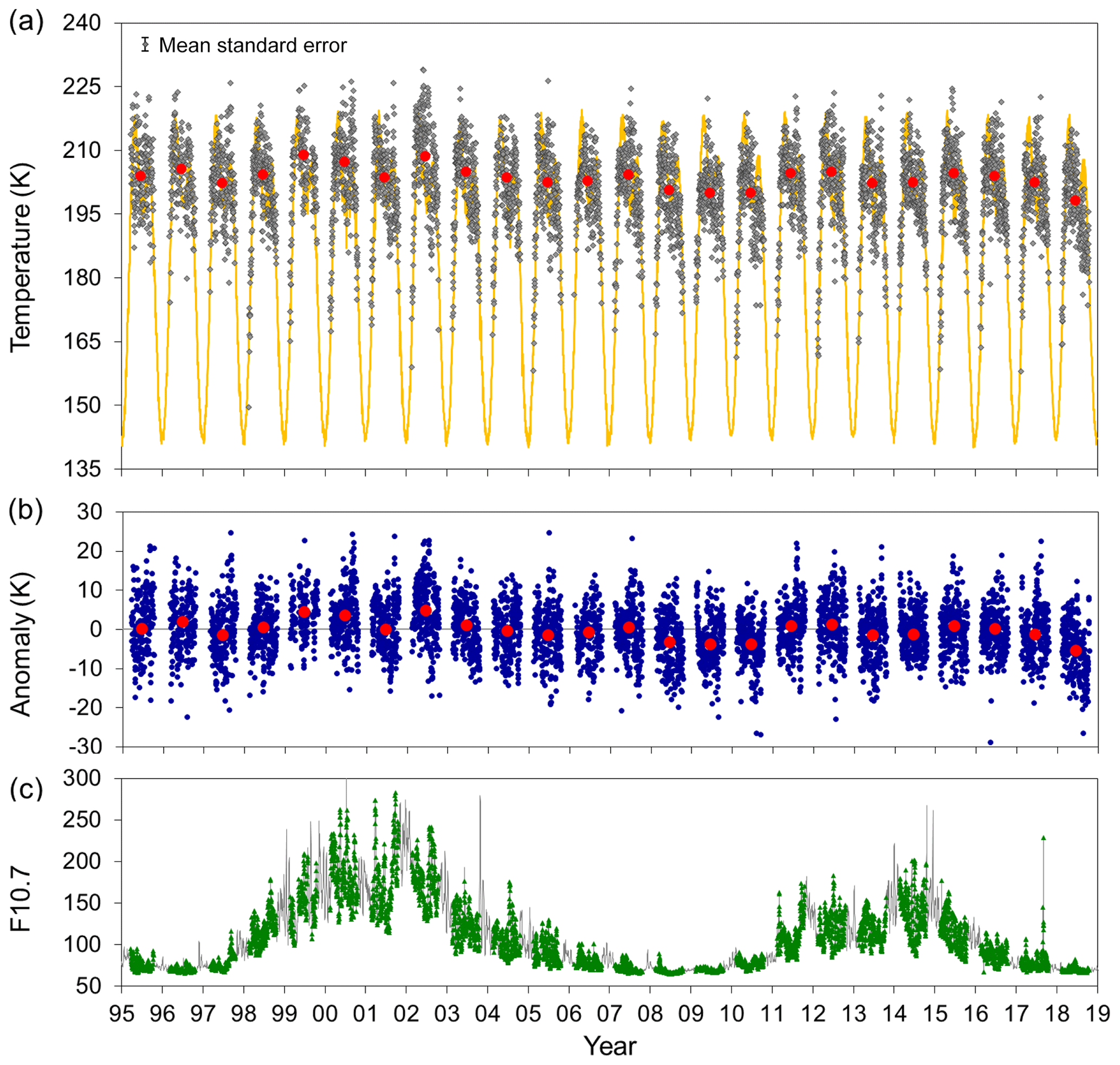
Figure 1(a) Davis nightly mean temperatures (grey dots; 5309 samples) and winter mean temperatures (D106-259; red points) plotted over the NRL-MSISE00 model temperature for 68∘ S (87 km altitude, local midnight values) for seasonal reference (Picone et al., 2002; gold line). (b) Nightly mean and winter mean temperature anomalies derived by subtracting the climatological mean (see text). (c) Daily mean F10.7 cm solar flux index (green points correspond to Davis OH temperature samples over the grey line, which are all daily observations).
A climatological mean is derived from a fit to the superposition of nightly mean temperatures for all annual series (Fig. 2). The climatological mean is characterised by a rapid autumn transition (February–March) increasing at 1.2 K d−1 until a turn-over on about 29 March (day of year D088), a slow winter decline (April–September) of −0.4 K d−1 that is punctuated by mid-April (∼ D113) and mid-August (∼ D227) dips corresponding to reversals in the mean meridional flow (Murphy et al., 2007), followed by a rapid spring transition (October–November) of −1.0 K d−1. Subtracting the climatological mean produces 5309 nightly mean temperature anomalies. Winter mean temperatures are calculated over the interval from 15 April (D106) to 15 September (D259), which avoids the winter-to-summer transition intervals and lower numbers of nightly observations due to the shorter night length in March and October. A seasonal fit (annual amplitude 41.9 K, semi-annual 23.0 K, terannual 7.5 K; green line) and the NRL-MSISE00 reference atmosphere (87 km altitude, local midnight values for Davis; gold points) are also added to Fig. 2 for reference and comparison. The model is limited in its representation of the seasonal cycle as only annual and semi-annual terms are modelled.
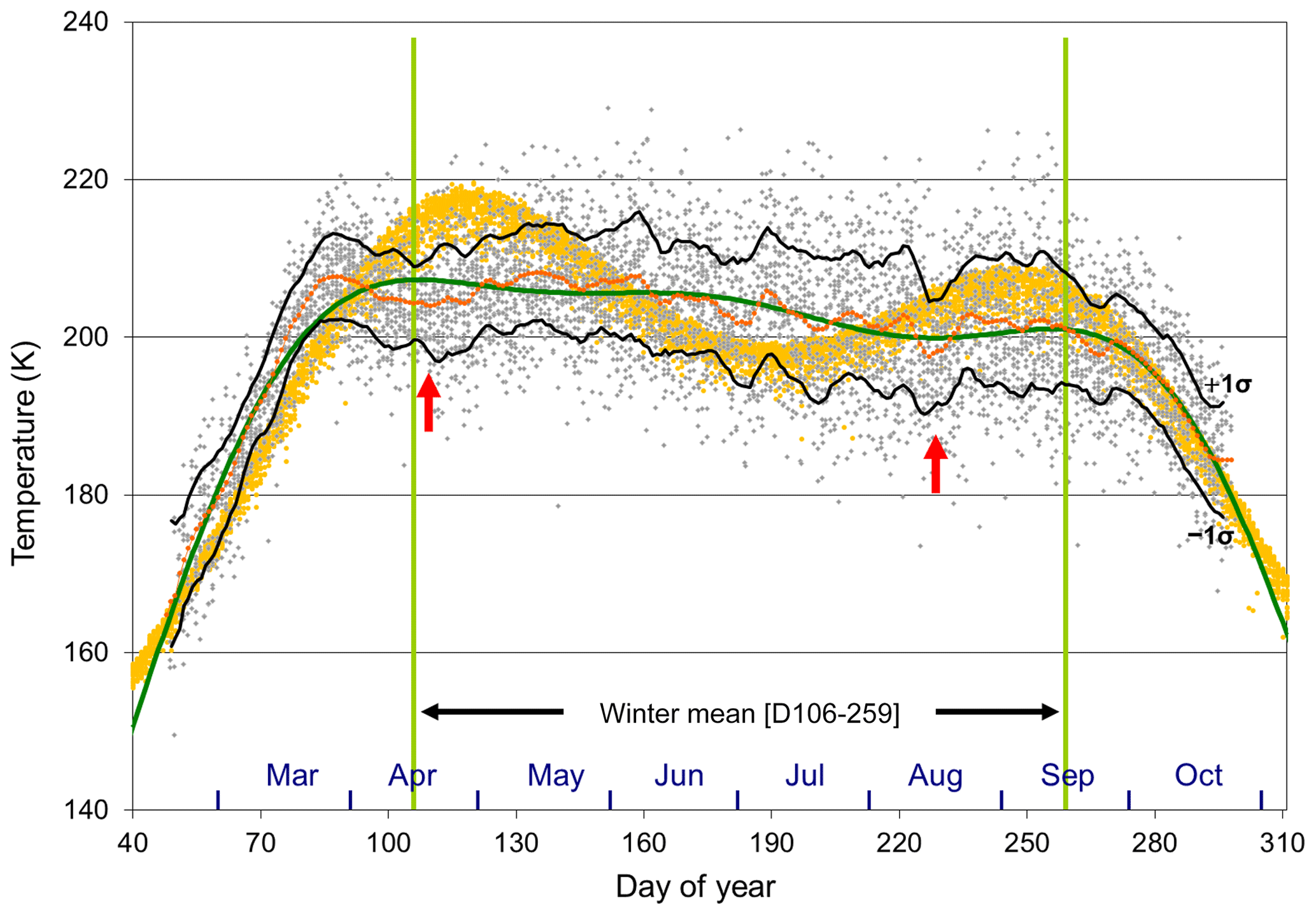
Figure 2Superposed nightly mean temperatures from 1995 to 2018 (grey points) and a 5 d running mean which represents the climatological mean (orange line) with 1σ intervals (black lines). The seasonal variation (annual, semi-annual, terannual fit; green line) and mid-April and mid-August dips (red arrows) are also indicated. Green vertical lines mark the calculation region for winter mean temperatures (avoiding spring and autumn transition intervals). The NRL-MSISE00 reference atmosphere (local midnight values for Davis) is also added for comparison (gold points).
4.1 Davis winter mean trends
Winter mean temperature anomalies over the 24 years of observations are plotted in Fig. 3a. The time series is fitted with a linear model containing a solar cycle term (F10.7) and long-term linear trend. This model yields a solar cycle response coefficient (S) of 4.30±1.02 K per 100 sfu (95 % confidence limits 2.2 K per 100 sfu <S<6.4 K per 100 sfu) and a long-term linear trend (L) of K per decade (95 % confidence limits −0.14 K per decade <L<−2.26 K per decade) and accounts for 58 % of the temperature variability.
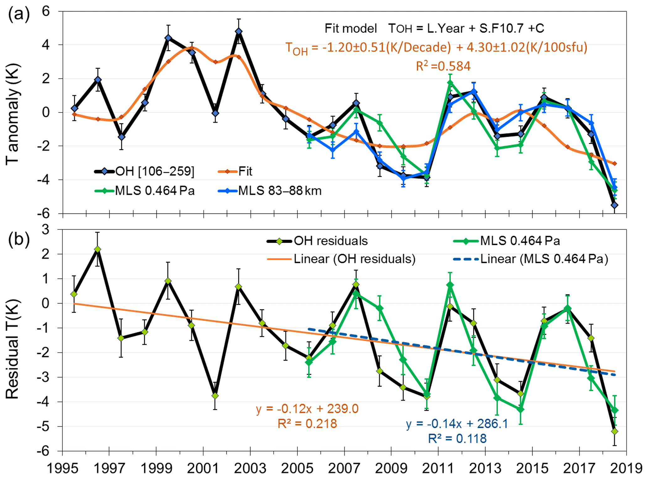
Figure 3(a) Winter mean (D106-259) temperature anomalies (black line) for Davis station (68∘ S, 78∘ E) fitted with a linear model containing a solar cycle term (F10.7cm flux) and long-term linear trend (orange line). Fit coefficients are 4.30±1.02 K per 100 sfu (95 % confidence limits 2.18 to 6.42 K per 100 sfu) and K per decade (95 % confidence limits −0.14 to −2.26 K per decade) and account for 58 % of the temperature variability. Also plotted (from 2005) are Aura/MLS temperature anomalies derived from the AMJJAS means of all satellite observations within 500 km of Davis station. (b) As for (a), but with the solar cycle component removed to better reveal the long-term trend and quasi-quadrennial oscillation (QQO). OH residuals (black line) are compared with Aura/MLS temperature residuals at the 0.00464 hPa level, corrected with the same solar cycle component as used for the Davis OH measurements.
The stability of trend coefficients were tested for the presence of sampling gaps in the OH temperature record. With the exception of 1999, when two intervals D095-126 and 213-249 were used to scan the OH(8-3) band, and 1996 lacking D176-202, all other years only have more than 85 % nights within the winter averaging window sampled (i.e. 85 % of the nights have a valid nightly average temperature with at least 10 measurements that pass selection criteria). A sample bias could be introduced in computing the anomalies if there was a significant departure from the climatological mean in those intervals. The test examined the effect on the derived coefficients by omitting individual years sequentially from the model fit computation. These show the range of L and S coefficients if a data gap for the entire winter interval was missing in a particular year. All coefficients derived from the omitted year computations remained within the uncertainty limits of the solar cycle and long-term trend coefficients when all years were included.
We report that a new record-low winter-mean temperature of 198.3 K was set for the Davis measurements in 2018, which is 1.7 K below the previous minimum recorded in 2009 (200.0 K). This is not entirely due to the low solar activity in 2018 (winter mean flux of 70.4 sfu) as both 2008 (66.9 sfu) and 2009 (69.1 sfu) had lower mean flux and the comparable years 1996 (70.6 sfu) and 2007 (71.9 sfu) was 7.4 K (205.7 K) and 6.1 K warmer (204.4 K) respectively.
Extracting the solar cycle contribution from the time series yields the long-term linear trend and residual variability plotted in Fig. 3b. It is apparent from this plot that a significant oscillation on an approximately 4-year (quasi-quadrennial) timescale remains. A least-squares fit of a sinusoid function to the data yields a period of 4.2 years and peak–peak amplitude of ∼3 K. This feature will be examined in detail in Part 2 of this work (French et al., 2020).
Distributions of the nightly mean residual temperatures for each year are shown for comparison in Fig. 4. The histogram colour scale indicates the winter mean temperature from the warmest year (1999; red) to the coldest year (2018; blue). Distributions vary between years from sharp normal distributions (e.g. 1998, 2007, 2016) to broad flat distributions (e.g. 1996, 1997) to skewed or double-peaked distributions (e.g. 2004, 2012, 2014, 2018). These differences can be attributed to the variability in large-scale planetary wave activity from year to year (French and Klekociuk, 2011).

Figure 4Histograms of nightly mean residual temperatures showing the distribution about the mean winter temperature (given in top right corner) coloured from red (warmest year: 1999) to blue (coldest year: 2018).
4.2 Seasonal variability in trends
Seasonal trend coefficients are examined using a 60 d sliding window and also from monthly average anomalies. Figure 5 shows the seasonal variability in solar cycle and long-term trend coefficients as compared to the winter mean trends (D106-259, 154 d mean; red lines) derived for Fig. 3. Seasonal solar response shows a maximum in May–June (∼5 K per 100 sfu) and a minimum around August (∼2 K per 100 sfu). Note that April and August temperatures are affected by the characteristic dips seen in the climatological mean during these months (see Fig. 2). Linear trend coefficients show maximum cooling responses in April–May ( K per decade) and in August–October ( K per decade). Virtually no long-term cooling trend is apparent for the midwinter months of June–July.
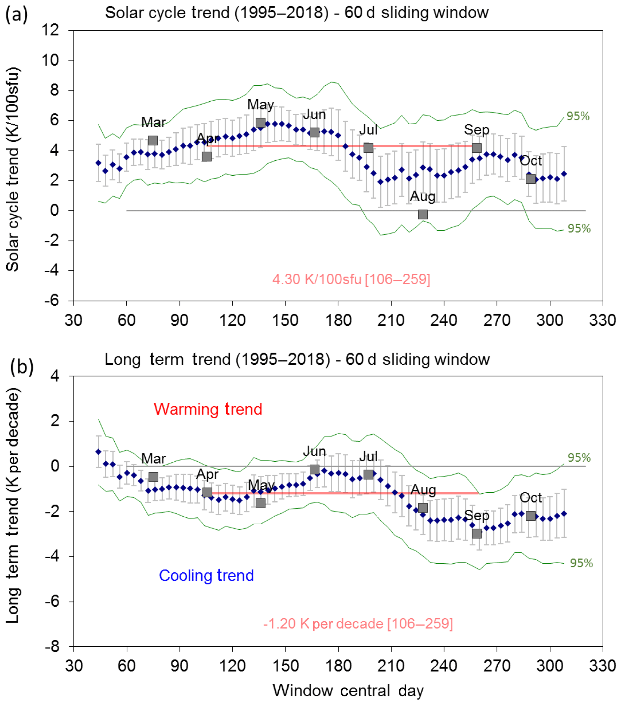
Figure 5The seasonal variability in (a) solar cycle and (b) long-term trend coefficients derived using a 60 d sliding window (blue dots) and as monthly trends (grey boxes) compared to the winter mean trends (red lines) derived for Fig. 3. The green lines show the confidence limits (95 %) for the trend coefficients.
4.3 Aura/MLS trend comparison
For comparison with the Davis trend measurements, we use version v4.2 level-2 data from the Microwave Limb Sounder (MLS) instrument on the Earth Observing System Aura satellite launched in July 2004 (Schwartz et al., 2008). Aura/MLS provides almost complete global coverage (82∘ S–82∘ N) of limb scanned vertical profiles (∼5–100 km) of temperature and geopotential height derived from the thermal microwave emissions near the spectral lines 118 GHz O2 and 234 GHz O18O. Previous comparisons of these data with MLS v2.2 temperatures were conducted by French and Mulligan (2010).
Overplotted in Fig. 3a (extending from 2005) are the equivalent Aura/MLS mean temperature anomalies computed by averaging all observations within 500 km of Davis, for the months of April to September (AMJJAS) over altitudes 83–88 km (blue line, obtained from a linear interpolation of Aura/MLS geopotential height profiles to geometric height in 1 km steps) and at the 0.00464 hPa (native Aura/MLS retrieval) pressure level (green line). The Aura/MLS data were selected according to the quality control recommendations described in Livesey et al. (2018). Approximately 60 samples per month (∼2 per day) are coincident within this range. We see very close agreement with both the pressure and interpolated altitude coordinates, considering that at these altitudes the vertical resolution (FWHM of the averaging kernel) of Aura/MLS in approximately 15 km (Schwartz et al., 2008), compared to the ∼8 km FWHM integration of the hydroxyl layer temperatures. The Aura/MLS measurements closely follow the solar response, the long-term linear trend, and the magnitude and period of the quasi-quadrennial oscillation (QQO).
We prefer the use of Aura/MLS pressure level data for the comparison with OH temperatures since it is the concentration (density) of reacting species that governs the hydroxyl layer position (primarily collisional quenching with O2 and N2 on the bottom side of the layer and reaction with atomic oxygen on the top side of the layer; e.g. Xu et al., 2012). Statistically (from a chi-squared fit to the anomalies), the closest agreement is with the 0.00464 hPa pressure level, and this is overplotted in Fig. 3b, corrected using the same solar cycle response that was determined from the Davis OH measurements. The linear long-term trend fit for Aura/MLS over 14 years is K per decade which compares very well to K per decade for the 24 years of Davis OH measurements, considering the seasonal variability shown above (Sect. 4.2) and the underlying QQO residual evident in both series, which has a significant effect on the fit over the different data spans.
We examine the QQO feature in greater detail in the second part of this work (French et al., 2020), but here, given the close agreement of Davis and Aura/MLS 0.00464 hPa trends in Fig. 3b, we apply the same model fit procedure to derive the Aura/MLS solar cycle and linear long-term trend coefficients to obtain a global picture of trends at the hydroxyl layer equivalent pressure level (0.00464 hPa). Figure 6 shows global trends determined by averaging Aura/MLS pressure level 0.00464 hPa temperature anomalies into a (latitude × longitude) grid, over Southern Hemisphere (SH) winter months (April–September; AMJJAS; panel a, trend; panel c, solar response) compared to Northern Hemisphere (NH) winter months (October–March; ONDJFM; panel (b) trend; panel (d) solar response). Each grid box has been corrected for the solar cycle response determined from a linear regression of temperature to F10.7 over the 14 years of Aura/MLS measurements. The long-term linear trend (panels a and b) and solar cycle response (panels c and d) for each grid box, together with their corresponding zonal means are presented. The maps contain some interesting features; enhanced bands of solar activity response occur at mid-latitudes in both winter hemispheres, although they are strongest in the SH (colour scales are the same for each hemisphere). Minima in sensitivity to solar forcing occur over the Equator and the poles. Long-term trends over the Aura/MLS era are not globally uniform. While the global mean trend for the SH winter (AMJJAS) is −0.31 K per decade, there are regions of warming, notably around the Equator, southern Africa, Europe, and the Atlantic Ocean, and the strongest cooling is found over Antarctica and northern Canada. For the NH winter (ONDJFM) the global mean is −0.11 K per decade with generally global cooling, except for warming over Antarctica, Europe, southern Africa, and the northern Pacific Ocean.
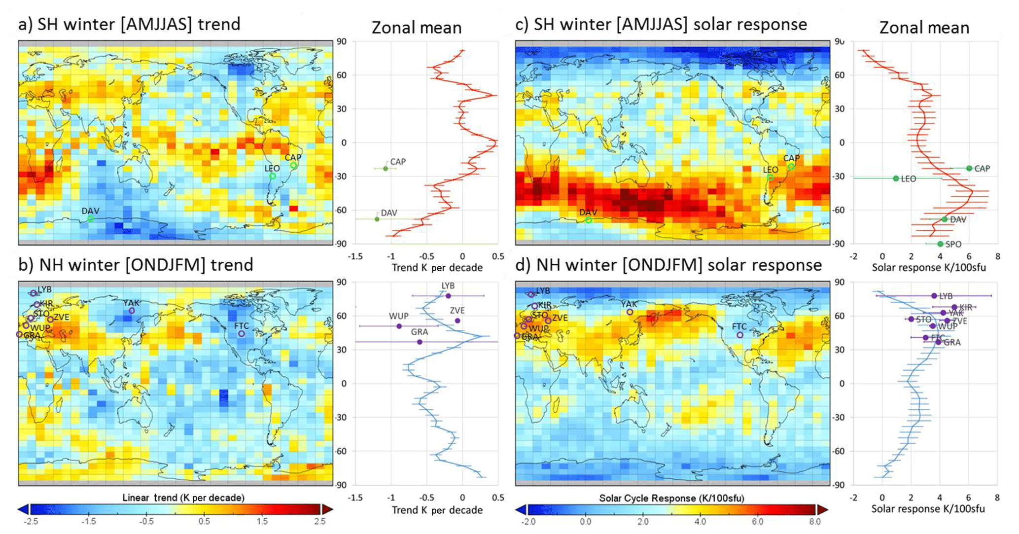
Figure 6Global temperature trends (a, b) and solar cycle responses (c, d), together with their corresponding zonal means determined from 14 years of MLS v4.2 pressure level 0.0046 hPa (hydroxyl layer equivalent), averaged into a 5∘ latitude × 10∘ longitude grid, and over Southern Hemisphere winter months (AMJJAS; a, c) compared to Northern Hemisphere winter months (ONDJFM; b, d). The linear trend and solar cycle response coefficients have been derived individually for each grid box from Aura/MLS over 14 years with no lag. Station locations indicate the Aura/MLS comparison, with ground-based observations of long-term trend and solar response given in Table 1.
4.4 Trend comparisons with other ground-based observations
It is useful to compare these Aura/MLS-derived solar response and trend coefficients with other observations, carefully bearing in mind that these observations may span different time intervals than available in the Aura/MLS measurement epoch. At Davis the solar cycle response (indicated by the green point and label DAV in Fig. 6c) determined over 24 years matches well with the zonal mean at 68∘ S determined from the Aura/MLS measurements. Davis appears to be on the poleward boundary of the strong band of solar sensitivity (∼40–70∘ S) in the SH winter. The long-term trend at Davis is marked by the green point and label DAV in panel a in Fig. 6 and, as we have seen from Fig. 3, agrees well with Aura/MLS.
Table 1 summarises the data span, derived long-term trend, and solar cycle coefficients from a collection of ground-based observers. Where new results are available these have been updated from Table 2 in French and Klekociuk (2011) and as compiled in Beig et al. (2008). Solar cycle and long-term trend coefficients from these sites are also marked in Fig. 6 where possible. The majority of these observations agree well (within error estimates) with the Aura/MLS zonal mean solar response and long-term trends evaluated here, given the different measurement epochs and geographic variability in the trends coefficients shown by Aura/MLS.
Table 1A comparison of solar cycle response and temperature trend observations from the ground-based OH observer network with updates since 2011 where available.

As some observers have found, there is an important question about a time delay in the OH layer temperature response to solar forcing via the various solar absorption mechanisms in the atmosphere. The major absorbers and altitude of solar extreme ultraviolet radiation are molecular oxygen (Schumann–Runge continuum, 80–130 km; Schumann–Runge electronic and vibrational bands, 40–95 km; Herzberg continuum, below 50 km) and ozone (Hartley–Huggins bands, below 50 km).
We have previously found a lag of around 160 d (F10.7 leads temperature) is best fit to the linear model (French and Klekociuk, 2011); others have found shorter lags: 80 d at Longyearbyen, Svalbard (Holmen et al., 2014); some have found larger lags: 25 months at Maimaga station, Yakutia (Ammosov et al., 2014; Reisin et al., 2014). Recalculating the long-term trends for Aura/MLS assuming a uniform global solar response (as for Davis) or with a 160 d lag and zonal mean solar response does not significantly change the warming and cooling patterns shown in Fig. 2, but the lag does reduce the cooling trend (on average by 0.16 K per decade for the Southern Hemisphere winter and 0.11 K per decade for the Northern Hemisphere winter) and increases the fit error. Beig (2011a, b), in their reviews of long-term trends in the temperature of the mesosphere and lower thermosphere (MLT), highlight the difficulty of distinguishing between the anthropogenic and solar cycle influences. In their results, mesopause region temperature trends were found to be either slightly negative or zero. At that time, it was believed that the solar response becomes stronger with increasing latitude in the mesosphere with typical values in the range of a few degrees per 100 solar flux units in the lower part of the mesosphere but reaching 4–5 K per 100 sfu near the mesopause. More recent studies using longer data sets (Ammosov et al., 2014; Holmen et al., 2014; Perminov et al., 2018) and satellite data (Tang et al., 2016) have reinforced that view.
Trend breaks began to appear in mesopause region temperatures in 2006 (Offermann et al., 2006, 2010), and these continue until now in certain locations (e.g. Jacobi et al., 2015; Kalicinsky et al., 2018; Yuan et al., 2019). These can be quite varied from site to site, ranging from −10 to +5 K per decade. Some of these estimates simply suffer from lack of observations (measurement spans less than a solar cycle). Few are longer than two solar cycles, but those of note are included in Table 1. OH temperature trend studies in the Southern Hemisphere are less common. Reid et al. (2017) report MLT-region nightglow intensities, temperatures, and emission heights near Adelaide (35∘ S, 138∘ E), Australia. Five years (2001–2006) of spectrometer measurements using OH(6-2) and O2(0-1) temperature are compared with 2 years of Aura/MLS data and 4.5 years of SABER data. Venturini et al. (2018) report mesopause region temperature variability and its trend in southern Brazil (Santa Maria, 30∘ S, 54∘ W), based on SABER data over the period 2003–2014. Nath and Sridharan (2014) examined the response of the middle atmosphere temperature to variations in solar cycle, QBO, and ENSO in the altitude range of 20–100 km and 10–15∘ N latitude using monthly averaged zonal mean SABER observations for the years 2002–2012. They found cooling trends in most of the stratosphere and the mesosphere (40–90 km). In the mesosphere, they found the temperature response to the solar cycle to be increasingly positive above 40 km. The temperature response to ENSO was found to be negative in the middle stratosphere and positive in the lower and upper stratosphere, whereas it appeared largely negative in the height range of 60–80 km and positive above 80 km.
5.1 Relationship between Davis trends and CO2 and O3 change
Our updated trend assessment over 24 years yields a cooling rate of K per decade for the mean winter (D106-259) temperatures in the hydroxyl layer above Davis. A slightly greater rate of K per decade is derived if the full year (D040-310) of observations is included in the annual means. Over the same period, annual mean surface CO2 volume mixing ratios (VMRs) increased from 360.82 ppm (1995) to 408.52 ppm (2018) (Mauna Loa values from Global Greenhouse Gas Reference Network https://www.esrl.noaa.gov/gmd/ccgg/trends/, last access: 15 May 2020), an increase of 47.7 ppm or 13.2 % (19.9 ppm per decade or 5.5 % per decade). Qian et al. (2019) quote a CO2 trend figure of 5.2 % per decade (or 5.1 % if the seasonal variation is removed before the linear trend calculated) based on measurements made by TIMED/SABER from 2002 to 2015. If the primary factor for the observed temperature trend is considered to be CO2 radiative cooling, a coefficient of −0.06 K per ppm CO2 or −0.22 K per % CO2 is implied. This is approximately twice the value obtained by Huang (2018) (her Fig. 2) who employed a linear scaling of the result of a doubling of CO2 concentration by Roble and Dickinson (1989). A CO2 increase of 26.5 % from 1960 to 2015 was accompanied by a temperature decrease of 1.4 % at an altitude of 89.4 km near Salt Lake City, Utah (18∘ N, 290∘ E).
CO2 is well mixed through the lower atmosphere with a constant VMR of up to about 80 km. Above this height, diffusion and photolysis processes begin to have an effect, reducing the VMR (Garcia et al., 2014), but these processes vary with latitude and season (Rezac et al., 2015; López-Puertas et al., 2017).
In a recent summary of progress in trends in the upper atmosphere, Laštovička (2017) identified greenhouse gases, particularly CO2 as the primary driver of long-term trends there. The overall effect of greenhouse gases at mesospheric altitudes is radiative cooling. The important secondary trend drivers in the mesosphere and lower thermosphere (MLT) are stratospheric ozone, water vapour concentration, and atmospheric dynamics. Temperature trends are predominantly negative, and recent progress in understanding the magnitude of the cooling has arisen from confirmation and quantification of the role of ozone. Lübken et al. (2013) present the results of trend studies in the mesosphere in the period 1961–2009 from the Leibniz-Institute Middle Atmosphere (LIMA) chemistry-transport model, which is driven with European Centre for Medium–Range Weather Forecasts (ECMWF) reanalysis below 40 km, and observed variations in CO2 and O3. They find that CO2 is the main driver of temperature change in the mesosphere, with O3 contributing approximately one-third to the trend. Linear temperature trends were found to vary substantially depending on the time period chosen primarily due to the influence of the complicated temporal variation in ozone. Figure 3 of Lübken et al. (2013) shows a monotonically increasing trend in CO2 compared with a much more complicated temporal ozone variation (essentially constant until 1980, a rapid decrease from 1980 to 1995, followed by an increase since then). Trends in ozone vary as a function of both altitude and latitude, with positive trends dominating in the lower stratosphere and mesosphere (Laštovička, 2017). Increases in water vapour concentration are considered a secondary but non-negligible effect, particularly in the lower thermosphere (Akmaev et al., 2006). The trend effect of dynamics was found to be very slightly negative in the mesosphere but very small compared with the radiatively induced trends. At the mesopause, the trend due to dynamics was positive and significantly larger (∼1 K per decade). These results were found to be in good agreement with observations from lidars, stratospheric sounding units (SSU) (Randall et al., 2009), and radio reflection heights which have decreased by more than 1 km in the last 50 years due to shrinking in the stratosphere or lower mesosphere caused by cooling.
The Whole Atmosphere Community Climate Model (WACCM) extended into the thermosphere (upper boundary ∼700 km) (WACCM-X) was used by Qian et al. (2019) (with the lower atmosphere constrained by reanalysis data) to investigate temperature trends and the effect of solar irradiance on temperature trends in the mesosphere during the period 1980–2014. The overall temperature trend in the mesopause region at 85 km was statistically insignificant at K per decade. Solar irradiance effects on the global average temperature are positive and decrease monotonically with decreasing altitude from a value of ∼3 K per 100 sfu in the lower thermosphere to ∼1 K per 100 sfu at 55 km. This is readily explained by the decreasing external energy from the Sun with reducing altitude. A monthly mean global average trend of 2.46 K per 100 sfu is quoted for the mesopause near 85 km. The mesosphere is affected by solar irradiance directly from local heating through absorption of radiation and indirectly through dynamics by its effects on the geostrophic winds which control the upward propagation of gravity waves and planetary waves generated in the troposphere. Zonal mean temperatures show significant variability as a function of altitude, latitude, and season. Qian et al. (2019) provide zonally averaged temperature trend values as a function of altitude (50–110 km) and latitude for each month (their Fig. 3), some of which are statistically significant. Solar cycle effects on temperature are in reasonable agreement with the Davis coefficients (shown in Fig. 5a) with positive values ranging from ∼3 to 5 K per 100 sfu, the largest values occurring in July and October (compare Qian et al., 2019 Fig. 4). The long-term trend is predominantly negative with values in the range of −1 to −3 K per decade with the largest cooling occurring in March and September at the latitude and altitude of the OH temperatures measured at Davis station. WACCM-X shows slightly positive trend values in the months of February, November, and December at Davis station, but OH(6-2) temperature data are not available in these months. The September maximum in cooling is in reasonable agreement with the Davis measurements shown in Fig. 5 of this work.
More recent results from Garcia et al. (2019) using WACCMv4 free-running (coupled ocean) simulations for the period 1955–2100 using IPCC RCP 6.0 attribute the changes in the trends of the temperature profile to monotonic increases in CO2 concentration together with a decrease in O3 until 1995 followed by a subsequent increase. Garcia et al. (2019) assign half of the stratopause negative temperature trend to ozone-depleting substances. At the mesopause, the global mean trend in temperature is approximately −0.6 K per decade. Solar cycle signals at the mesopause are in the range of 2–3 K per 100 sfu with slightly higher values in the southern polar cap. Very large seasonal trends in temperature at all altitudes are associated with the development of the Antarctic ozone hole. Trends are largest in the November–December period, and teleconnections are made with the upper mesosphere via gravity wave (GW) filtering by the zonal wind anomaly in the southern polar cap.
5.2 Trend breaks
When analysing long-term trends, several authors (Lübken et al., 2013; Qian et al., 2019) emphasise the importance of specifying the length of the time period, as well as the beginning and end of the period, because trend drivers can be different for different periods (e.g. Yuan et al., 2019). Yuan et al. (2019) report long-term trends of the nocturnal mesopause temperature and altitude from lidar observations at mid-latitude (41–42∘ N, 105–112∘ W) in the period 1990–2018. They divided their observations into two categories: the high mesopause (HM) above 97 km during the non-summer months, mainly formed by radiative cooling, and the low mesopause (LM) below 92 km during the non-winter months generated by mostly by adiabatic cooling. This idea of the mesopause at two different altitudes is well established (e.g. von Zahn et al., 1996; Xu et al., 2007; Thulasiraman and Nee, 2002). Although Yuan et al. (2019) obtained a cooling trend of more than 2 K per decade in the mesopause temperature along with a decreasing trend in mesopause height since 1990, the temperature trend has been statistically insignificant since 2000.
Trend breaks have been reported at other mid-latitude stations (Offermann et al., 2006, 2010), where a discontinuity was found in the overall trend in the year 2001–2002. Using some of the same data as Offermann et al. (2006), Kalicinsky et al. (2016) reported a trend break in the middle of 2008. Before the break point, there is a clear negative trend reported to be K per decade, whereas after 2008, a large positive trend of 6.4±3.3 K per decade is determined. Two possible explanations are suggested for the trend break: the first is that it is the result of a combination of the solar cycle and a long-period oscillation such as the 22-year Hale cycle of the Sun. A second possible explanation of the very substantial change in the trend at 2008 is a combination of the solar flux with a sensitivity of 4.1±0.8 K per 100 sfu together with a long-period oscillation of 24–26 years with an amplitude of about 2 K. Kalicinsky et al. (2018) find support for this idea in the identification of a quasi-decadal oscillation in the summer mesopause over western Europe in plasma-scale height observations (near 80 km altitude), which are in anti-correlation with the potential oscillation in temperature from OH* measurements. The anti-correlation in the two data sets is explained on the basis of the fact that they originate below (plasma-scale height data) and above (OH* temperature data) the temperature minimum in the mesopause region in summer. Jacobi et al. (2015) find that the long-term behaviour of both meridional and zonal winds at 90–95 km in northern mid-latitude stations exhibits trend breaks in summer near 1999, although the winter data are well described by a single linear trend over the years 1980–2015. We find no obvious sign of a discontinuity in the trend obtained in the Davis data from 1995 to 2018. There is no significant change in the long-term trend or solar response when extending the period of study from 16 years (2005–2010 coefficients 4.79±1.02 K per 100 sfu and K per decade; French and Klekociuk, 2011) to 24 years (this work). Neither coefficient has changed outside the uncertainty.
5.3 Effect of changes in the OH* layer height
There is widespread acceptance that cooling of the middle atmosphere due to increases in CO2 concentration has resulted in shrinking of the middle atmosphere (e.g. Grygalashvyly et al., 2014; Sonnemann et al., 2015). This does raise the question, however, of whether the OH* layer is fixed to a constant pressure level rather than a constant altitude. There are mixed reports on this topic. In a long-term study of the effects of chemistry, greenhouse gases, and the solar modulation on OH* layer trends using the Leibniz Institute Middle Atmosphere (LIMA) chemistry-transport model covering the period 1969 to 2009, Grygalashvyly et al. (2014) reported a downward shift in the OH* layer by about 0.3 km per decade in all seasons due to shrinking of the middle atmosphere resulting from radiative cooling by increasing CO2 concentrations. Wüst et al. (2017) report a descent in the mean altitude of the OH* layer of 0.02 km yr−1 from 14 years of SABER data (2002–2015) in the alpine region of southern Europe (44–48∘ N, 6–12∘ E). They refer to a paper by Bremer and Peters (2008) which reports low-frequency reflection heights (ca. 80–83 km) between 1959 and 2006 and derive a figure of 0.032 km yr−1.
Sivakandan et al. (2016) have published a long-term variation paper on OH peak emission altitude and volume emission rate over Indian low latitudes using SABER data. A weak decreasing trend of 19.56 m yr−1 was reported for the peak emission altitude of the night-time OH* layer. García-Comas et al. (2017) reported a slightly larger decrease of 40 m per decade in SABER OH volume emission rate weighted altitude at mid-latitudes, which accompanied a 0.7 % per decade increase in OH intensity and a 0.6 K per decade decrease in OH equivalent temperature.
A vertical shift of the OH* layer either upward or downward gives rise to a change in the emission-weighted temperature, which is measured by ground-based optical instruments (French and Mulligan, 2010; Liu and Shepherd, 2006; von Savigny, 2015). Von Savigny (2015) reported no apparent trend or solar cycle in OH emission altitude at the local time of the SCIAMACHY night-time observations in the period 2003–2011. However, Teiser and von Savigny (2017) found evidence of an 11-year solar cycle in the vertically integrated emission rate and in the centroid emission altitude of both the OH(3-1) and OH(6-2) bands in SCIAMACHY data. Gao et al. (2016) found no evidence that the OH* peak heights are affected by solar cycle in 13 years of TIMED/SABER data and deduced that the solar cycle variation in temperature obtained from ground-based OH nightglow observations was essentially immune from the OH emission altitude variations. Huang (2018) found no systematic response of airglow O(1S) green line, O2(0-1), or OH(8-3) VER peak heights with the F10.7 solar cycle using two airglow models OHCD and MACD-90. The Huang (2018) result is supported by Gao et al. (2016) using TIMED/SABER data and by von Savigny (2015) using SCIAMACHY data. These confirmations of the remarkable long-term stability of the peak altitude of the OH* layer in an atmosphere with increasing CO2 concentration and changing solar radiation are essential for the use of long-term studies of mesopause region temperatures derived from ground-based OH* optical measurements.
We have examined the altitude variation in the OH* layer over Davis during the period 2002–2018 using the OH-B channel volume mission rate (VER) from TIMED/SABER (version 2.0) sensitive in the wavelength range of 1.56–1.72 µm, which includes mostly the OH(4-2) and OH(5-3) bands. All VER altitude profiles between day 105 and day 259 that satisfied the selection criteria (tangent point within 500 km of Davis and solar zenith angle >97∘), employed by French and Mulligan (2010), were used to determine the altitude of the layer. The altitude of the peak was obtained from a Gaussian profile fitted to the VER profile (for more details, see French and Mulligan, 2010). The slope of the best-fit line to the winter annual average peak altitude was km yr−1 as shown in Fig. 7, i.e. no significant change in altitude of the layer over the period in agreement with the result of Gao et al. (2016).
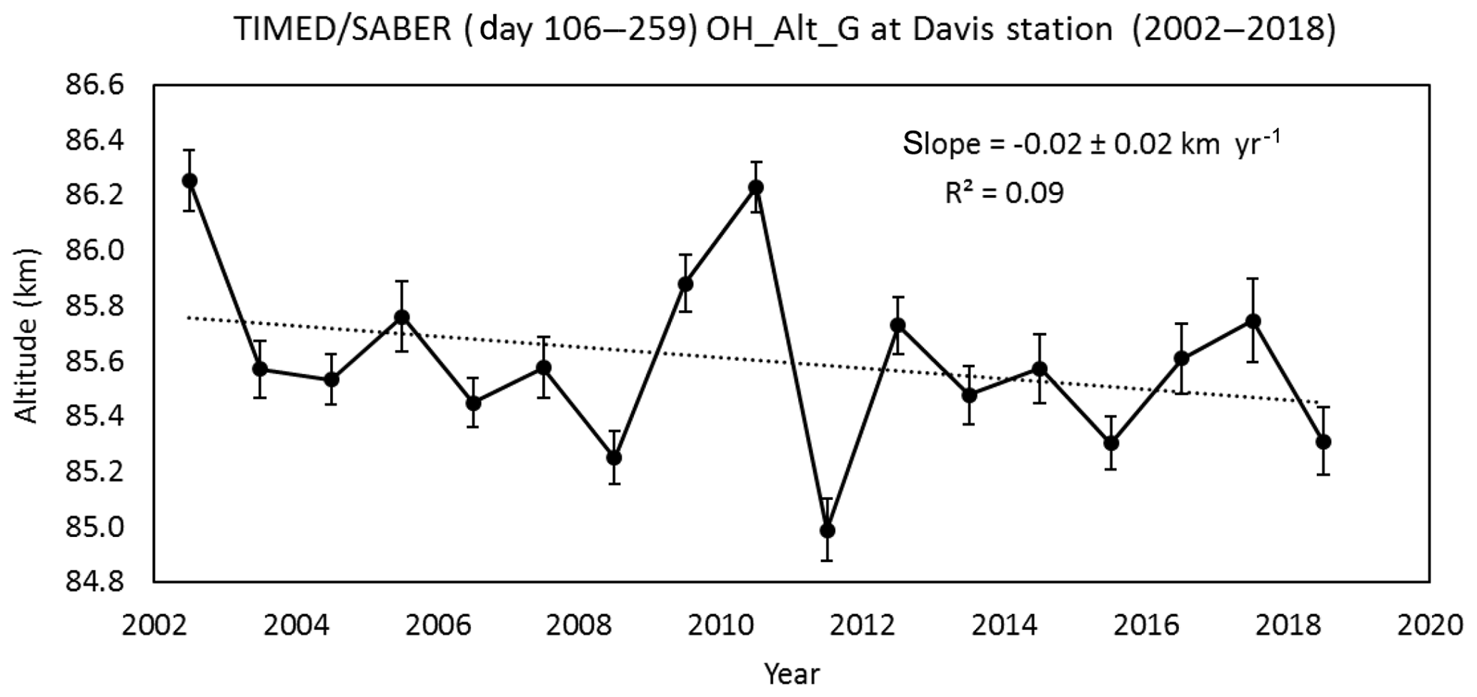
Figure 7The trend in the mean winter OH layer altitude, derived from TIMED/SABER (version 2.0) OH-B channel volume emission rate. The slope of the best-fit line is km yr−1, i.e. no significant change in altitude of the layer over this interval.
5.4 Global solar cycle and long-term trends
The long-term trend measured at Davis is well matched with the result from Aura/MLS over 14 years for the Southern Hemisphere winter months (AMJJAS) at the 0.00464 hPa level. Clearly though, applying the same analysis to the global temperature field reveals that trends are far from globally uniform (Fig. 6). In the SH winter the most significant cooling trends are seen over the southern polar cap and northern Canada, with warming trends over southern Africa, around the Equator and over Europe and Russia. NH winter cooling trends are strongest over eastern Russia and North America, but warming trends remain over Europe.
There are a number of limitations and assumptions made for these derived trends: (i) there are only 14 years from which to extract a solar cycle component; (ii) a solar cycle component is computed for each grid box – the zonal means calculated are generally within 2 K per 100 sfu of other reported solar response coefficients, but there is a strong latitudinal and seasonal dependence (strongest solar flux response in mid-latitude winter hemisphere – near-zero response in high-latitude summer); (iii) we have assumed no lag between solar flux variations and the temperature response, whereas previous work for the Davis response for example indicates a ∼160 d lag is optimal at least for Davis (French and Klekociuk, 2011); and (iv) for comparison with other hydroxyl temperature long-term trends we assume the global OH layer height is well matched with the Aura/MLS 0.00464 hPa level.
To address uncertainties about the solar response coefficient (item ii above) we have recalculated the global trends assuming a fixed response for each grid box (4.2 K per 100 sfu as derived from the Davis observations) and also as zonal means but for a lag of 160 d (F10.7 leads T) as previously found for Davis. This analysis determines that, by and large, the warming and cooling patterns observed in Fig. 6 do not change significantly for the different solar cycle response computations.
While the WACCM-X results presented by Qian et al. (2019) are in reasonable agreement with the OH temperature behaviour measured at Davis station, the zonally averaged pattern of solar cycle response and linear trend obtained from WACCM-X differs considerably from that obtained from the analysis of the Aura/MLS data at the 0.00464 hPa level shown in Fig. 6. In the Aura/MLS results, the solar response in both hemispheres in winter shows a great deal more variation as a function of latitude than is evident in the WACCM-X results at 87 km (Fig. 4 of Qian et al., 2019). The zonally averaged Aura/MLS pattern shows maxima (∼6 K per 100 sfu) in southern mid-latitudes in the SH winter and similarly a maximum (although a smaller peak ∼4 K per 100 sfu compared to the SH response) in northern mid-latitudes in the NH winter. The solar cycle response is essentially zero at 82∘ north and south during the NH winter months, but it is of the order of 3 K per 100 sfu at 82∘ south in SH winter. The SH winter months have the largest variation, with a pronounced maximum in the latitude range of ∼10 to 40∘ S. (The maximum also shows longitudinal structure with a much broader maximum between 90∘ east and 90∘ west which is centred at higher southern latitudes.) Several authors (Perminov et al., 2014; Pertsev and Perminov, 2008) have reported that winter OH* temperatures are more sensitive to the solar flux variation than summer temperatures, and this agrees with the Aura/MLS variation shown here.
The long-term trend modelled by WACCM-X is predominantly negative or zero at the altitude of the OH layer (87 km) at all latitudes and in all months apart from February, November, and December, when a positive trend of up to ∼3 K per decade is present at high southern latitudes (see Fig. 3 in Qian et al., 2019). Aura/MLS results also show a predominantly slightly negative trend ∼0.5–1 K per decade, except at the Equator, and at mid-latitudes in the SH winter months.
Solomon et al. (2018) simulated the anthropogenic global change through the entire atmosphere using WACCM-X in a free-running mode (i.e. lower atmosphere below 50 km not constrained by ECMWF reanalysis data) using constant low solar activity conditions. They find substantial cooling in the mesosphere of the order of −1 K per decade, increasing to −2.8 K per decade in the thermosphere. Temperature decreases were small near the mesopause compared with the variation in the annual mean, thus making trends there somewhat uncertain. Solomon et al. (2018) conclude that inconsistent observational results in the mesopause region, together with little or no global mean trends is due to the dominance of dynamical processes in controlling mesopause temperature, which exhibits significant inter-annual variability, even without variable solar forcing.
The SABER data set (2002–2015) was used by Tang et al. (2016) to study the response of the cold-point temperature of the mesopause (T-CPM) to solar activity. The results showed that the T-CPM is significantly correlated to solar activity at all latitudes, and the solar response becomes stronger with increasing latitude. The solar-cycle dependence of the mesopause cold-point temperature (T-CPM) is due to the relative importance of CO2 and NO infrared cooling (Tang et al., 2016). NO density at solar maximum is about 3 times that at solar minimum. Consequently, CO2 cooling is relatively less important at solar maximum but is the dominant cooling mechanism during solar minimum.
Values of the solar response of T-CPM reported by Tang et al. (2016) increased from 2.82±0.73 K per 100 sfu at 0–10∘ S to 6.35±1.16 K per 100 sfu at 60–70∘ S (see their Fig. 5a). Correlation coefficients of mesopause temperature with F10.7 cm solar irradiance data were higher for mid-latitudes (>0.9) than at the Equator (∼0.7) and at higher latitude (see their Fig. 5b). The correlation coefficient found for 70∘ S (∼0.8) is consistent with the value obtained for the OH* temperatures (Fig. 3a) (R2=0.584 or R=0.76) obtained in this work. At low latitudes, one would expect the QBO and ENSO to be significant factors (see, e.g., Nath and Sridharan, 2014), but at high latitudes, gravity wave activity is a candidate for the missing variance. Inter-annual variations in GWs at high latitudes are correlated with the strength of the polar vortex. A stronger polar vortex filters out more eastward propagating GWs, thus leading to more westward GW drag, which drives stronger meridional circulation (Karlsson and Shepherd, 2018).
Although the altitude of the mesospheric cold-point changes with season (e.g. Yuan et al., 2019) and tends to be higher than the centroid height of the OH* layer, the global solar response value obtained for T-CPM (4.89±0.67 K per 100 sfu) is in good agreement with the solar response coefficient derived from ground-based OH* observations.
The solar response of the T-CPM in Tang et al. (2016) shows some significant differences from the results in Fig. 6 (zonal mean cycle from Aura/MLS) of this work. The solar response of the T-CPM increases more or less monotonically with latitude, whereas the solar response observed by Aura/MLS maximises at higher mid-latitudes. Of course the height of the T-CPM is some 7 km higher on average, as indicated in Fig. 9b of Tang et al. (2016).
As a final comment on the global trends, it is noted that the largest errors in the linear trend fit for the SH winter understandably occur coincident with the regions positively or negatively correlated with the QQO (not shown here). The fit can be significantly improved if the QQO component can be understood and modelled. We investigate the QQO in detail in Part 2 of this work.
We provide updates for the long-term trend and solar cycle response derived from 24 years of spectrometer observations of hydroxyl airglow at Davis research station, Antarctica (68∘ S, 78∘ E). A cooling trend in the mean winter temperatures (D106-259) of K per decade (95 % confidence limits −0.14 K per decade <L<−2.26 K per decade) is obtained coupled with a solar cycle response coefficient of 4.30±1.02 K per 100 sfu (95 % confidence limits 2.2 K per 100 sfu <S<6.4 K per 100 sfu). The observed cooling is consistent with radiative cooling due to increasing CO2 concentrations and a rate of −0.06 K per ppm CO2 or −0.22 K per % CO2 is implied (ignoring possible contributions of stratospheric ozone change to the trend). A significant note is that a new record-low winter-mean temperature was set for the Davis measurements in 2018, with a value of 198.3 K, which is 1.7 K below the previous minimum recorded in 2009 (200.0 K). An examination of the seasonal variation in the trend fit parameters reveals that very little (no significant) long-term trend occurs over the 2 midwinter months of June and July, but 95 % significant trends of −1.5 to −2.6 K per decade occur during the April–May and August–October intervals. From an examination of TIMED/SABER VER profiles we see no evidence that the trend results obtained can be significantly attributed to a change in the height of the OH layer.
We do not see evidence of a trend break or a change in the nature of the underlying trend after accounting for the solar cycle response in the Davis OH temperatures; however, this simple solar-cycle and linear trend model fit accounts for only 58 % of the temperature variability. The remaining variability reveals evidence of a temperature oscillation on a quasi-quadrennial (∼4-year period) timescale.
We compare our observations with Aura/MLS version v4.2 level-2 data over the last 14 years when these satellite data are available and find close agreement (a best fit to the variance in mean winter anomaly) with the 0.00464 hPa (native Aura/MLS retrieval) pressure level values. The solar cycle response, long-term trend, and underlying QQO residuals are consistent with the Davis observations. Consequently, we derive global maps of Aura/MLS trend and solar response coefficients for the SH and NH winter periods to compare with other observers and models. Significant patterns for the zonally averaged solar cycle response are maxima in southern mid-latitudes in the SH winter and in northern mid-latitudes in the NH winter. Long-term trends are predominantly slightly negative (∼0.5–1 K per decade), except at the Equator and at mid-latitudes in the SH winter months. Comparisons are also made with the WACCM-X model and mesopause cold-point temperature versus a solar activity study using TIMED/SABER data of Tang et al. (2016), both of which reveal significant differences in the zonally averaged patterns of solar cycle response and linear trend compared to the Aura/MLS data at 0.00464 hPa.
Further analysis using the data sets described here is undertaken to explore the QQO signal revealed in the residual temperatures. A second part of this paper (French et al., 2020) concerns this observation.
All Davis hydroxyl rotational data described in this paper are available through the Australian Antarctic Data Centre website (project no. AAS4157) via the following link https://data.aad.gov.au/metadata/records/Davis_OH_airglow (Burns and French, 2002). The satellite data used in this paper were obtained from the Aura/MLS data centre (see https://mls.jpl.nasa.gov, Schwartz et al., 2008), and the SABER data centre (see http://saber.gats-inc.com/data.php, Russell et al., 1999) and are publicly available.
WJRF managed data collection, performed data analysis, and prepared the paper with contributions from all co-authors.
FJM was responsible for the analysis of SABER data, manuscript editing, figures, and references.
ARK was responsible for the analysis of Aura/MLS satellite data and manuscript editing.
The authors declare that they have no conflict of interest.
The authors thank the dedicated work of the Davis optical physicists and engineers over many years in the collection of airglow data and calibration of instruments.
We thank both the Aura/MLS and TIMED/SABER science teams for the use of the global satellite data as described in data availability.
We acknowledge the efforts of the Network for Detection of Mesospheric Change (https://ndmc.dlr.de/, last access: 14 May 2020) in coordinating research to understand mesospheric change processes.
This work is undertaken within the Australian Antarctic Program (project AAS 4157) under the Australian Government Department of Agriculture, Water and the Environment.
This paper was edited by Franz-Josef Lübken and reviewed by two anonymous referees.
Akmaev, R. A., Fomichev, V. I., and Zhu, X.: Impact of middle-atmospheric composition changes on greenhouse cooling in the upper atmosphere, J. Atmos. Sol.-Terr. Phys., 68, 1879–1889, https://doi.org/10.1016/j.jastp.2006.03.008, 2006.
Ammosov, P., Gavrilyeva, G., Ammosova, A., and Koltovskoi, I.: Response of the mesopause temperatures to solar activity over Yakutia in 1999–2013, Adv. Sp. Res., 54, 2518–2524, https://doi.org/10.1016/J.ASR.2014.06.007, 2014.
Azeem, S. M. I., Sivjee, G. G., Won, Y.-I., and Mutiso, C.: Solar cycle signature and secular long-term trend in OH airglow temperature observations at South Pole, Antarctica, J. Geophys. Res.-Sp. Phys., 112, A01305, https://doi.org/10.1029/2005JA011475, 2007.
Beig, G.: Trends in the mesopause region temperature and our present understanding-an update, Phys. Chem. Earth, 31, 3–9, https://doi.org/10.1016/j.pce.2005.03.007, 2006.
Beig, G.: Long-term trends in the temperature of the mesosphere/lower thermosphere region: 1. Anthropogenic influences, J. Geophys. Res.-Sp. Phys., 116, A00H11, https://doi.org/10.1029/2011JA016646, 2011a.
Beig, G.: Long-term trends in the temperature of the mesosphere/lower thermosphere region: 2. Solar response, J. Geophys. Res.-Sp. Phys., 116, A00H12, https://doi.org/10.1029/2011JA016766, 2011b.
Beig, G., Keckhut, P., Lowe, R. P., Roble, R. G., Mlynczak, M. G., Scheer, J., Fomichev, V. I., Offermann, D., French, W. J. R., Shepherd, M. G., Semenov, A. I., Remsberg, E. E., She, C. Y., Lübken, F. J., Bremer, J., Clemesha, B. R., Stegman, J., Sigernes, F., and Fadnavis, S.: Review of mesospheric temperature trends, Rev. Geophys., 41, 1015, https://doi.org/10.1029/2002RG000121, 2003.
Beig, G., Scheer, J., Mlynczak, M. G., and Keckhut, P.: Overview of the temperature response in the mesosphere and lower thermosphere to solar activity, Rev. Geophys., 46, RG3002, https://doi.org/10.1029/2007RG000236, 2008.
Bengtsson, L., Hagemann, S., and Hodges, K. I.: Can climate trends be calculated from reanalysis data?, J. Geophys. Res., 109, D11111, https://doi.org/10.1029/2004JD004536, 2004.
Bremer, J. and Peters, D.: Influence of stratospheric ozone changes on long-term trends in the meso- and lower thermosphere, J. Atmos. Sol. Terr. Phys., 70, 1473–1481, 2008.
Brooke, J. S. A., Bernath, P. F., Western, C. M., Sneden, C., Afşar, M., Li, G., and Gordon, I. E.: Line strengths of rovibrational and rotational transitions in the X 2 Π ground state of OH, J. Quant. Spectrosc. Ra., 168, 142–157, https://doi.org/10.1016/j.jqsrt.2015.07.021, 2016.
Burns, G. and French, J.: Rotational temperature studies of the hydroxyl airglow layer above Davis, Antarctica, Ver. 8, Australian Antarctic Data Centre, available at: https://data.aad.gov.au/metadata/records/Davis_OH_airglow/ (last access: 15 May 2020), 2002.
Burns, G. B., Kawahara, T. D., French, W. J. R., Nomura, A., and Klekociuk, A. R.: A comparison of hydroxyl rotational temperatures from Davis (69∘ S, 78∘ E) with sodium lidar temperatures from Syowa (69∘ S, 39∘ E), Geophys. Res. Lett., 30, 1025, https://doi.org/10.1029/2002GL016413, 2003.
Clemesha, B., Takahashi, H., Simonich, D., Gobbi, D., and Batista, P.: Experimental evidence for solar cycle and long-term change in the low-latitude MLT region, J. Atmos. Sol.-Terr. Phys., 67, 191–196, https://doi.org/10.1016/j.jastp.2004.07.027, 2005.
Espy, P. J., Ochoa Fernández, S., Forkman, P., Murtagh, D., and Stegman, J.: The role of the QBO in the inter-hemispheric coupling of summer mesospheric temperatures, Atmos. Chem. Phys., 11, 495–502, https://doi.org/10.5194/acp-11-495-2011, 2011.
Fomichev, V. I., Jonsson, A. I., de Grandpré, J., Beagley, S. R., McLandress, C., Semeniuk, K., and Shepherd, T. G.: Response of the middle atmosphere to CO2 doubling: Results from the Canadian middle atmosphere model, J. Clim., 20, 1121–1144, https://doi.org/10.1175/JCLI4030.1, 2007.
French, W. J. R. and Burns, G. B.: The influence of large-scale oscillations on long-term trend assessment in hydroxyl temperatures over Davis, Antarctica, J. Atmos. Sol.-Terr. Phys., 66, 493–506, https://doi.org/10.1016/j.jastp.2004.01.027, 2004.
French, W. J. R. and Klekociuk, A. R.: Long-term trends in Antarctic winter hydroxyl temperatures, J. Geophys. Res., 116, D00P09, https://doi.org/10.1029/2011JD015731, 2011.
French, W. J. R. and Mulligan, F. J.: Stability of temperatures from TIMED/SABER v1.07 (2002–2009) and Aura/MLS v2.2 (2004–2009) compared with OH(6-2) temperatures observed at Davis Station, Antarctica, Atmos. Chem. Phys., 10, 11439–11446, https://doi.org/10.5194/acp-10-11439-2010, 2010.
French, W. J. R., Burns, G. B., Finlayson, K., Greet, P. A., Lowe, R. P., and Williams, P. F. B.: Hydroxyl (6-2) airglow emission intensity ratios for rotational temperature determination, Ann. Geophys., 18, 1293–1303, https://doi.org/10.1007/s00585-000-1293-2, 2000.
French, W. J. R., Klekociuk, A. R., and Mulligan, F. J.: Analysis of 24 years of mesopause region OH rotational temperature observations at Davis, Antarctica – Part 2: Evidence of a quasi-quadrennial oscillation (QQO) in the polar mesosphere, Atmos. Chem. Phys., in review, 2020.
Gao, H., Xu, J., and Chen, G.: The responses of the nightglow emissions observed by the TIMED/SABER satellite to solar radiation, J. Geophys. Res.-Sp. Phys., 121, 1627–1642, https://doi.org/10.1002/2015JA021624, 2016.
García-Comas, M., López-González, M. J., González-Galindo, F., de la Rosa, J. L., López-Puertas, M., Shepherd, M. G., and Shepherd, G. G.: Mesospheric OH layer altitude at midlatitudes: variability over the Sierra Nevada Observatory in Granada, Spain (37∘ N, 3∘ W), Ann. Geophys., 35, 1151–1164, https://doi.org/10.5194/angeo-35-1151-2017, 2017.
Garcia, R. R., López-Puertas, M., Funke, B., Marsh, D. R., Kinnison, D. E., Smith, A. K., and González-Galindo, F.: On the distribution of CO2 and CO in the mesosphere and lower thermosphere, J. Geophys. Res., 119, 5700–5718, https://doi.org/10.1002/2013JD021208, 2014.
Garcia, R. R., Yue, J., and Russell, J. M.: Middle atmosphere temperature trends in the 20 th and 21 st centuries simulated with the Whole Atmosphere Community Climate Model (WACCM), J. Geophys. Res.-Sp. Phys., 124, 7984–7993, https://doi.org/10.1029/2019ja026909, 2019.
Greet, P. A., French, W. J. R., Burns, G. B., Williams, P. F. B., Lowe, R. P., and Finlayson, K.: OH(6-2) spectra and rotational temperature measurements at Davis, Antarctica, Ann. Geophys., 16, 77–89, https://doi.org/10.1007/s00585-997-0077-3, 1997.
Grygalashvyly, M., Sonnemann, G. R., Lübken, F. J., Hartogh, P., and Berger, U.: Hydroxyl layer: Mean state and trends at midlatitudes, J. Geophys. Res. Atmos., 119, 12391–12419, https://doi.org/10.1002/2014JD022094, 2014.
Holmen, S. E., Dyrland, M. E., and Sigernes, F.: Mesospheric temperatures derived from three decades of hydroxyl airglow measurements from Longyearbyen, Svalbard (78∘ N), Acta Geophys., 62, 302–315, https://doi.org/10.2478/s11600-013-0159-4, 2014.
Huang, T.-Y.: Influences of CO2 increase, solar cycle variation, and geomagnetic activity on airglow from 1960 to 2015, J. Atmos. Sol.-Terr. Phys., 171, 164–175, https://doi.org/10.1016/J.JASTP.2017.06.008, 2018.
Jacobi, C., Lilienthal, F., Geißler, C., and Krug, A.: Long-term variability of mid-latitude mesosphere-lower thermosphere winds over Collm (51∘ N, 13∘ E), J. Atmos. Sol.-Terr. Phys., 136, 174–186, https://doi.org/10.1016/j.jastp.2015.05.006, 2015.
Kalicinsky, C., Knieling, P., Koppmann, R., Offermann, D., Steinbrecht, W., and Wintel, J.: Long-term dynamics of OH * temperatures over central Europe: trends and solar correlations, Atmos. Chem. Phys., 16, 15033–15047, https://doi.org/10.5194/acp-16-15033-2016, 2016.
Kalicinsky, C., Peters, D. H. W., Entzian, G., Knieling, P., and Matthias, V.: Observational evidence for a quasi-bidecadal oscillation in the summer mesopause region over Western Europe, J. Atmos. Sol.-Terr. Phys., 178, 7–16, https://doi.org/10.1016/j.jastp.2018.05.008, 2018.
Karlsson, B. and Shepherd, T. G.: The improbable clouds at the edge of the atmosphere, Phys. Today, 71, 30–36, https://doi.org/10.1063/PT.3.3946, 2018.
Kim, G., Kim, J.-H., Kim, Y. H., and Lee, Y. S.: Long-term trend of mesospheric temperatures over Kiruna (68∘ N, 21∘ E) during 2003–2014, J. Atmos. Sol.-Terr. Phys., 161, 83–87, https://doi.org/10.1016/j.jastp.2017.06.018, 2017.
Kvifte, G.: Temperature measurements from OH bands, Planet, Space Sci., 5, 153–157, https://doi.org/10.1016/0032-0633(61)90090-3, 1961.
Langhoff, S. R., Werner, H. J., and Rosmus, P.: Theoretical Transition Probabilities for the OH Meinel System, J. Mol. Spectrosc., 118, 507–529, 1986.
Laštovička, J.: A review of recent progress in trends in the upper atmosphere, J. Atmos. Sol.-Terr. Phys., 163, 2–13, https://doi.org/10.1016/j.jastp.2017.03.009, 2017.
Liu, G. and Shepherd, G. G.: An empirical model for the altitude of the OH nightglow emission, Geophys. Res. Lett., 33, L09805, https://doi.org/10.1029/2005GL025297, 2006.
Livesey, N. J., Read, W. G., Wagner, P. A., Froidevaux, L., Lambert, A., Manney, G. L., Millán Valle, L. F., Pumphrey, H. C., Santee, M. L., Schwartz, M. J., Wang, S., Fuller, R. A., Jarnot, R. F., Knosp, B. W., Martinez, E., and Lay, R. R.: Earth Observing System (EOS) Aura Microwave Limb Sounder (MLS) Version4.2x Level 2 data quality and description document Version 4.2x–3.1, 1–163, available at: https://mls.jpl.nasa.gov/data/v4-2_data_quality_document.pdf (last access: 15 May 2020), 2018.
López-Puertas, M., Funke, B., Jurado-Navarro, A., García-Comas, M., Gardini, A., Boone, C. D., Rezac, L., and Garcia, R. R.: Validation of the MIPAS CO2 volume mixing ratio in themesosphere and lower thermosphere and comparison with WACCM simulations, J. Geophys. Res., 122, 8345–8366, https://doi.org/10.1002/2017JD026805, 2017.
Lübken, F.-J., Berger, U., and Baumgarten, G.: Temperature trends in the midlatitude summer mesosphere, J. Geophys. Res.-Atmos., 118, 13347–13360, https://doi.org/10.1002/2013JD020576, 2013.
Mertens, C. J., Mlynczak, M. G., López-Puertas, M., Wintersteiner, P. P., Picard, R. H., Winick, J. R., Gordley, L. L., and Russell III, J. M.: Retrieval of kinetic temperature and carbon dioxide abundance from nonlocal thermodynamic equilibrium limb emission measurements made by the SABER experiment on the TIMED satellite, Proc SPIE 4882, Remote Sensing of Clouds and the Atmosphere VII, 162–171, 2003.
Mies, F. H.: Calculated vibrational transition probabilities of OH(X2Π), J. Mol. Spectrosc., 53, 150–188, https://doi.org/10.1016/0022-2852(74)90125-8, 1974.
Mulligan, F. J., Dyrland, M. E., Sigernes, F., and Deehr, C. S.: Inferring hydroxyl layer peak heights from ground-based measurements of OH(6-2) band integrated emission rate at Longyearbyen (78∘ N, 16∘ E), Ann. Geophys., 27, 4197–4205, https://doi.org/10.5194/angeo-27-4197-2009, 2009.
Murphy, D. J., French, W. J. R., and Vincent, R. A.: Long-period planetary waves in the mesosphere and lower thermosphere above Davis, Antarctica, J. Atmos. Sol.-Terr. Phys., 69, 2118–2138, https://doi.org/10.1016/J.JASTP.2007.06.008, 2007.
Nath, O. and Sridharan, S.: Long-term variabilities and tendencies in zonal mean TIMED–SABER ozone and temperature in the middle atmosphere at 10–15∘ N, J. Atmos. Sol.-Terr. Phys., 120, 1–8, https://doi.org/10.1016/j.jastp.2014.08.010, 2014.
Noll, S., Winkler, H., Goussev, O., and Proxauf, B.: OH level populations and accuracies of Einstein-A coefficients from hundreds of measured lines, Atmos. Chem. Phys. Discuss., https://doi.org/10.5194/acp-2019-1102, in review, 2019.
Offermann, D., Jarisch, M., Donner, M., Steinbrecht, W., and Semenov, A. I.: OH temperature re-analysis forced by recent variance increases, J. Atmos. Sol.-Terr. Phys., 68, 1924–1933, https://doi.org/10.1016/J.JASTP.2006.03.007, 2006.
Offermann, D., Hoffmann, P., Knieling, P., Koppmann, R., Oberheide, J., and Steinbrecht, W.: Long-term trends and solar cycle variations of mesospheric temperature and dynamics, J. Geophys. Res., 115, D18127, https://doi.org/10.1029/2009JD013363, 2010.
Perminov, V. I., Semenov, A. I., Medvedeva, I. V., and Pertsev, N. N.: Temperature variations in the mesopause region according to the hydroxyl-emission observations at midlatitudes, Geomagn. Aeron., 54, 230–239, https://doi.org/10.1134/S0016793214020157, 2014.
Perminov, V. I., Semenov, A. I., Pertsev, N. N., Medvedeva, I. V., Dalin, P. A., and Sukhodoev, V. A.: Multi-year behaviour of the midnight OH* temperature according to observations at Zvenigorod over 2000–2016, Adv. Sp. Res., 61, 1901–1908, https://doi.org/10.1016/J.ASR.2017.07.020, 2018.
Pertsev, N. and Perminov, V.: Response of the mesopause airglow to solar activity inferred from measurements at Zvenigorod, Russia, Ann. Geophys., 26, 1049–1056, https://doi.org/10.5194/angeo-26-1049-2008, 2008.
Picone, J. M., Hedin, A. E., Drob, D. P., and Aikin, A. C.: NRLMSISE-00 empirical model of the atmosphere: Statistical comparisons and scientific issues, J. Geophys. Res.-Sp. Phys., 107, 1468, https://doi.org/10.1029/2002JA009430, 2002.
Qian, L., Jacobi, C., and McInerney, J.: Trends and Solar Irradiance Effects in the Mesosphere, J. Geophys. Res.-Sp. Phys., 124, 1343–1360, https://doi.org/10.1029/2018JA026367, 2019.
Randall, C. E., Harvey, V. L., Siskind, D. E., France, J., Bernath, P. F., Boone, C. D., and Walker K. A.: NOx descent in the Arctic middle atmosphere in early 2009, Geophys. Res. Lett., 36, L18811, https://doi.org/10.1029/2009GL039706, 2009.
Reid, I. M., Spargo, A. J., Woithe, J. M., Klekociuk, A. R., Younger, J. P., and Sivjee, G. G.: Seasonal MLT-region nightglow intensities, temperatures, and emission heights at a Southern Hemisphere midlatitude site, Ann. Geophys., 35, 567–582, https://doi.org/10.5194/angeo-35-567-2017, 2017.
Reisin, E. R., Scheer, J., Dyrland, M. E., Sigernes, F., Deehr, C. S., Schmidt, C., Höppner, K., Bittner, M., Ammosov, P. P., Gavrilyeva, G. A., Stegman, J., Perminov, V. I., Semenov, A. I., Knieling, P., Koppmann, R., Shiokawa, K., Lowe, R. P., López-González, M. J., Rodríguez, E., Zhao, Y., Taylor, M. J., Buriti, R. A., Espy, P. J., French, W. J. R., Eichmann, K.-U., Burrows, J. P., and von Savigny, C.: Traveling planetary wave activity from mesopause region airglow temperatures determined by the Network for the Detection of Mesospheric Change (NDMC), J. Atmos. Sol.-Terr. Phys., 119, 71–82, https://doi.org/10.1016/J.JASTP.2014.07.002, 2014.
Rezac, L., Jian, Y., Yue, J., Russell, J. M., Kutepov, A., Garcia, R., Walker, K., and Bernath, P.: Validation of the global distribution of CO2 volume mixing ratio in the mesosphere and lower thermosphere from SABER, J. Geophys. Res., 120, 12067–12081, https://doi.org/10.1002/2015JD023955, 2015.
Roble, R. G.: On the feasibility of developing a global atmospheric model extending from the ground to the exosphere, Washington DC American Geophysical Union Geophysical Monograph Series, edited by: Siskind, D. E., Eckermann, S. D., and Summers, M. E., 53–67, 2000.
Roble, R. G. and Dickinson, R. E.: How will changes in carbon dioxide and methane modify the mean structure of the mesosphere and thermosphere?, Geophys. Res. Lett., 16, 1441–1444, https://doi.org/10.1029/GL016i012p01441, 1989.
Russell III, J. M., Mlynczak, M. G., Gordley, L. L., Tansock Jr., J. J., and Esplin, R. W.: Overview of the SABER experiment and preliminary calibration results, Proc. SPIE 3756, Optical Spectroscopic Tech. Instrum. Atmos. Space Res. III, 277–288, https://doi.org/10.1117/12.366382, 1999 (data available at: http://saber.gats-inc.com/data.php, last access: 15 May 2020).
Scheer, J., Reisin, E. R., and Mandrini, C. H.: Solar activity signatures in mesopause region temperatures and atomic oxygen related airglow brightness at El Leoncito, Argentina, J. Atmos. Sol.-Terr. Phys., 67, 145–154, https://doi.org/10.1016/j.jastp.2004.07.023, 2005.
Schmidt, H., Brasseur, G. P., Charron, M., Manzini, E., Giorgetta, M. A., Diehl, T., Fomichev, V. I., Kinnison, D., Marsh, D., and Walters, S.: The HAMMONIA chemistry climate model: Sensitivity of the mesopause region to the 11-year solar cycle and CO2 doubling, J. Clim., 19, 3903–3931, https://doi.org/10.1175/JCLI3829.1, 2006.
Schwartz, M. J., Lambert, A., Manney, G. L., Read, W. G., Livesey, N. J., Froidevaux, L., Ao, C. O., Bernath, P. F., Boone, C. D., Cofield, R. E., Daffer, W. H., Drouin, B. J., Fetzer, E. J., Fuller, R. A., Jarnot, R. F., Jiang, J. H., Jiang, Y. B., Knosp, B. W., Krüger, K., Li, J.-L. F., Mlynczak, M. G., Pawson, S., Russell, J. M., Santee, M. L., Snyder, W. V., Stek, P. C., Thurstans, R. P., Tompkins, A. M., Wagner, P. A., Walker, K. A., Waters, J. W., and Wu, D. L.: Validation of the Aura Microwave Limb Sounder temperature and geopotential height measurements, J. Geophys. Res., 113, D15S11, https://doi.org/10.1029/2007jd008783, 2008 (data available at: https://mls.jpl.nasa.gov, last access: 15 May 2020).
Sivakandan, M., Ramkumar, T. K., Taori, A., Rao, V., and Niranjan, K.: Long-term variation of OH peak emission altitude and volume emission rate over Indian low latitudes, J. Atmos. Sol.-Terr. Phys., 138–139, 161–168, https://doi.org/10.1016/j.jastp.2016.01.012, 2016.
Sivjee, G. G.: Airglow hydroxyl emissions, Planet. Space Sci., 40, 235–242, https://doi.org/10.1016/0032-0633(92)90061-R, 1992.
Solomon, S. C., Liu, H., Marsh, D. R., McInerney, J. M., Qian, L., and Vitt, F. M.: Whole Atmosphere Simulation of Anthropogenic Climate Change, Geophys. Res. Lett., 45, 1567–1576, https://doi.org/10.1002/2017GL076950, 2018.
Sonnemann, G. R., Hartogh, P., Berger, U., and Grygalashvyly, M.: Hydroxyl layer: trend of number density and intra-annual variability, Ann. Geophys., 33, 749–767, https://doi.org/10.5194/angeo-33-749-2015, 2015.
Tang, C., Liu, D., Wei, H., Wang, Y., Dai, C., Wu, P., Zhu, W., and Rao, R.: The response of the temperature of cold-point mesopause to solar activity based on SABER data set, J. Geophys. Res.-Sp. Phys., 121, 7245–7255, https://doi.org/10.1002/2016JA022538, 2016.
Teiser, G. and von Savigny, C.: Variability of OH(3-1) and OH(6-2) emission altitude and volume emission rate from 2003 to 2011, J. Atmos. Sol.-Terr. Phys., 161, 28–42, https://doi.org/10.1016/J.JASTP.2017.04.010, 2017.
Thulasiraman, S. and Nee, J. B.: Further evidence of a two-level mesopause and its variations from UARS high-resolution Doppler imager temperature data, J. Geophys. Res., 107, 4355, https://doi.org/10.1029/2000JD000118, 2002.
Turnbull, D. N. and Lowe, R. P.: New hydroxyl transition probabilities and their importance in airglow studies, Planet. Space Sci., 37, 723–738, https://doi.org/10.1016/0032-0633(89)90042-1, 1989.
van der Loo, M. P. J. and Groenenboom, G. C.: Theoretical transition probabilities for the OH Meinel system, J. Chem. Phys., 126, 114314, https://doi.org/10.1063/1.2646859, 2007.
Venturini, M. S., Bageston, J. V., Caetano, N. R., Peres, L. V., Bencherif, H., and Schuch, N. J.: Mesopause region temperature variability and its trend in southern Brazil, Ann. Geophys., 36, 301–310, https://doi.org/10.5194/angeo-36-301-2018, 2018.
von Savigny, C.: Variability of OH(3-1) emission altitude from 2003 to 2011: Long-term stability and universality of the emission rate–altitude relationship, J. Atmos. Sol.-Terr. Phys., 127, 120–128, https://doi.org/10.1016/J.JASTP.2015.02.001, 2015.
von Savigny, C., McDade, I. C., Eichmann, K.-U., and Burrows, J. P.: On the dependence of the OH* Meinel emission altitude on vibrational level: SCIAMACHY observations and model simulations, Atmos. Chem. Phys., 12, 8813–8828, https://doi.org/10.5194/acp-12-8813-2012, 2012.
von Zahn, U., Höffner, J., Eska, V., and Alpers, M.: The mesopause altitude: Only two distinctive levels worldwide?, Geophys. Res. Lett., 23, 3231–3234, https://doi.org/10.1029/96GL03041, 1996.
Wüst, S., Bittner, M., Yee, J.-H., Mlynczak, M. G., and Russell III, J. M.: Variability of the Brunt–Väisälä frequency at the OH* layer height, Atmos. Meas. Tech., 10, 4895–4903, https://doi.org/10.5194/amt-10-4895-2017, 2017.
Xu, J., Liu, H.-L., Yuan, W., Smith, A. K., Roble, R. G., Mertens, C. J., Russell, J. M., and Mlynczak, M. G.: Mesopause structure from Thermosphere, Ionosphere, Mesosphere, Energetics, and Dynamics (TIMED)/Sounding of the Atmosphere Using Broadband Emission Radiometry (SABER) observations, J. Geophys. Res., 112, D09102, https://doi.org/10.1029/2006JD007711, 2007.
Xu, J., Gao, H., Smith, A. K., and Zhu, Y. :Using TIMED/SABER nightglow observations to investigate hydroxyl emission mechanisms in the mesopause region, J. Geophys.Res., 117, D02301, https://doi.org/10.1029/2011JD016342, 2012.
Yuan, T., Solomon, S. C., She, C.-Y., Krueger, D. A., and Liu, H. -L.: The long-term trends of nocturnal mesopause temperature and altitude revealed by Na lidar observations between 1990 and 2018 at mid-latitude, J. Geophys. Res.-Atmos., 124, 5970–5980, https://doi.org/10.1029/2018JD029828, 2019.