the Creative Commons Attribution 4.0 License.
the Creative Commons Attribution 4.0 License.
 | 28 May 2020
Aerosol indirect effects on the temperature–precipitation scaling
Sylvain Mailler
Philippe Drobinski
Aerosols may impact precipitation in a complex way involving their direct and indirect effects. In a previous numerical study, the overall microphysical effect of aerosols was found to weaken precipitation through reduced precipitable water and convective instability. The present study aims to quantify the relative importance of these two processes in the reduction of summer precipitation using temperature–precipitation scaling. Based on a numerical sensitivity experiment conducted in central Europe aiming to isolate indirect effects, the results show that, all others effects being equal, the scaling of hourly convective precipitation with temperature follows the Clausius–Clapeyron (CC) relationship, whereas the decrease in convective precipitation does not scale with the CC law since it is mostly attributable to increased stability with increased aerosol concentration rather than to decreased precipitable water content. This effect is larger at low surface temperatures at which clouds are statistically more frequent and optically thicker. At these temperatures, the increase in stability is mostly linked to the stronger reduction in temperature in the lower troposphere compared to the upper troposphere, which results in lower lapse rates.


The temperature–precipitation relationship has often been studied because it has been hypothesized to give insight into the change in precipitation in a warming climate. In this context, one may distinguish extreme precipitation studies from mean precipitation studies. The Clausius–Clapeyron (CC) law relates changes in temperature to changes in water vapour content assuming constant relative humidity:
where es is the water vapour saturation pressure, T is the temperature, Lv is the latent heat of vaporization, and Rv is the gas constant for air. It has been suggested that precipitation extremes correspond to events where the whole column of moisture is precipitated out and are therefore expected to scale with the CC law (Pall et al., 2007; Muller, 2013). However many deviations from CC scaling have been observed. The literature has described a peak-like shape for the temperature–precipitation extremes relationship with CC scaling for the cold season and negative scaling for the warm season (Drobinski et al., 2016). Sub-CC scaling for warm temperatures can be explained by either the decrease in relative humidity (Hardwick et al., 2010; Panthou et al., 2014), the decrease in precipitation duration (Utsumi et al., 2011; Singleton and Toumi, 2013; Panthou et al., 2014), the decrease in precipitation efficiency, or changes in dynamics (Drobinski et al., 2016). Conversely, Lenderink and van Meijgaard (2008) have found an increase in precipitation extremes (their 99.9th and 99th percentiles) beyond CC scaling for temperatures between 12 and 23∘C at De Bilt in the Netherlands. It has been argued that this “super-CC” scaling is due to the transition between stratiform and convective precipitation (Haerter and Berg, 2009; Berg and Haerter, 2013; Molnar et al., 2015) and enhanced dynamics in convective clouds at higher temperatures (Lenderink et al., 2017). Although less documented than extremes, a “hook shape” of the temperature–precipitation relationship, that is a positive slope at low temperatures and a negative slope at high temperatures, is also suggested for mean precipitation (Zhao and Khalil, 1993; Madden and Williams, 1978; Crhová and Holtanová, 2017; Rodrigo, 2019) as well as differences between land and sea areas (Adler et al., 2008; Trenberth and Shea, 2005). CC scaling is less expected for global mean precipitation, which is more constrained by an energetic budget than extreme precipitation (Allen and Ingram, 2002; Held and Soden, 2006; Muller et al., 2011; Muller, 2013). On the local scales, the energy budget includes a term accounting for the transport of dry static energy, which may suppress the constraint in many regions, as shown by Muller and O'Gorman (2011). The study of Hardwick et al. (2010) suggests that Australia belongs to the regions where the constraint still holds. Indeed, they have systematically found lower slopes for median precipitation than for extreme precipitation in their four selected in situ measurement stations in Australia.
The fact that the CC law is not always adequate for describing the temperature–precipitation relationship in a given climate does not mean that if one were to perturb the climate, the change in precipitation would not follow CC scaling. Indeed, using regional climate models (RCMs) in the Mediterranean region and within the framework of the HyMeX programme (Drobinski et al., 2014), Drobinski et al. (2018) found CC scaling between past and future climate while observing hook shapes for both past and future climate temperature–precipitation relationships. It has often been shown that extreme precipitation would increase at a rate similar to the CC law, whereas mean precipitation would increase at a lower rate in a warming climate (Allen and Ingram, 2002; Boer, 1993; Trenberth, 1998; Held and Soden, 2006).
Apart from greenhouse gas forcing, the forcing of aerosols is another feature that can modify climate and therefore the temperature–precipitation relationship. Aerosols affect climate through their direct and semi-direct effects as well as through their effects on cloud microphysics (indirect effects). While their direct effect is rather well understood, many uncertainties remain for the indirect effects. Stevens and Feingold (2009) described aerosol–cloud interactions as buffered systems in which many processes seem to partly compensate each other. Among these effects, the Twomey (1977) effect, also called the “first indirect effect”, is an increase in the cloud optical depth (COD) through reduced cloud droplet radius for constant liquid water content with increased aerosol concentration. Aerosol indirect effects may also increase cloud lifetime (Albrecht, 1989), but as of today no consensus exists on the reality of this effect (Small et al., 2009; Seifert et al., 2015; Malavelle et al., 2017), and its representation in climate models is highly dependent on the model's microphysical formulation (Zhou and Penner, 2017). Many hypotheses have been suggested for the effect of aerosols in convective clouds, such as convective invigoration (Khain et al., 2004, 2005; Rosenfeld et al., 2008; Lebo and Seinfeld, 2011; Fan et al., 2013), which would be the consequence of an increased release of latent heat due to ice formation associated with a decrease in warm rain formation with increased aerosol loads. Miltenberger et al. (2018) have, however, observed an invigoration of deep convective clouds below the freezing level, indicating that the previous theory may not hold under certain conditions. Instead, they proposed that the observed enhancement of precipitation once convection is organized is caused by reduced dry air entrainment in the convective core of polluted clouds. Aerosols were also hypothesized to affect precipitation through changes in cloud evaporation (Xue and Feingold, 2006; Dagan et al., 2015; Liu et al., 2019) or through changes in entrainment rates (Dagan et al., 2015; Miltenberger et al., 2018).
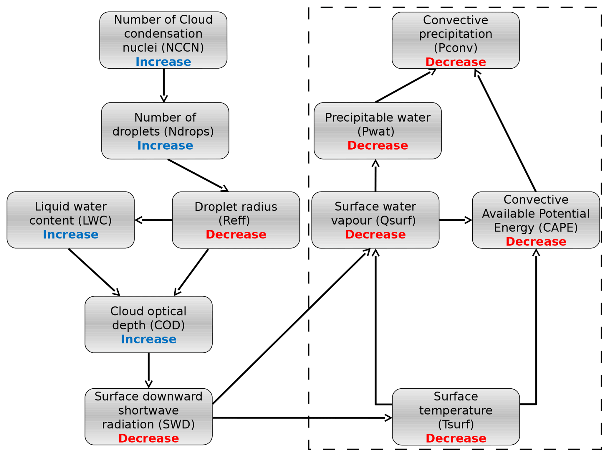
Figure 1Schematic summary of the aerosol causal sequence for the indirect effects of aerosols on convective precipitation (adapted from Da Silva et al., 2018). The dotted rectangle indicates the part of the scheme which is detailed in the present study.
A common feature of both direct and indirect effects of aerosols is a global decrease in precipitation through a decrease in evaporation from the surface due to the reduction of short-wave downwelling fluxes at the surface (Ramanathan et al., 2001; Lelieveld et al., 2002; Bollasina et al., 2011; Salzmann et al., 2014). Many modelling case studies may underestimate this longer-term feedback when performing short-time simulations or simulations in a small domain (Khain et al., 2004, 2005; Khain and Lynn, 2009; Lebo and Seinfeld, 2011; Lebo and Morrison, 2014; Lebo, 2014; Miltenberger et al., 2018). Conversely, long-term simulations are often performed at a coarse resolution using convective parameterizations that do not implement the microphysical effect of aerosols on convective clouds (Bollasina et al., 2011; Salzmann et al., 2014). Few studies take into account both the microphysical effects of aerosols on convection and the aerosol long-term radiative feedback by realizing high-resolution simulations over a few months (Morrison and Grabowski, 2011; Fan et al., 2013), which does not prevent uncertainties related to their representation by RCMs in these intermediate configurations. The study of Da Silva et al. (2018) over the Euro-Mediterranean area is one such study in which the decrease in surface precipitation was related to the radiative path previously described (see Fig. 1). The authors have shown that the consecutive surface cooling not only reduces the water content but also stabilizes the atmosphere as suggested by Fan et al. (2013), Morrison and Grabowski (2011), and Stjern et al. (2017), and hence acts to reduce precipitation with increased aerosol concentration. A third path is possible as a combination of these two paths since the reduction in water vapour mixing ratio at the surface would also contribute to increase the stability of the atmosphere through less latent heat released with increased aerosol concentrations. To our knowledge, an evaluation of the relative contribution of these paths to precipitation reduction due to aerosol indirect effects has not been proposed yet. This study aims to determine these contributions and therefore can be seen as a natural follow-up to Da Silva et al. (2018). For that purpose, we use the temperature–precipitation relationship, which appears to be a natural framework since both effects are a consequence of the decrease in surface temperature.
Section 2 details the configuration of the Weather Research and Forecasting Model (WRF) used, the simulations, and the method that have been performed for this sensitivity analysis. Section 3 analyses the temperature–precipitation scaling and quantifies each contribution to the reduction in central European summertime precipitation under the effect of a massive concentration of cloud condensation nuclei. Section 4 concludes the study.
2.1 Model configuration
Version 3.7.1 of the WRF (Skamarock et al., 2008) is used in this study. The model was run with a 50 km (low resolution; LR), a 16.6 km (medium resolution; MR), and a 3.3 km (high resolution; HR) horizontal resolution in a domain displayed in Fig. 2. It is forced by the Global Forecast System (GFS) model (National Centers for Environmental Prediction et al., 2000) as initial and boundary conditions. Temperature, humidity, geopotential, and velocity components are nudged towards GFS analysis data with a Newtonian-type method using a relaxation coefficient of s−1 as recommended by, for example, Salameh et al. (2010), Omrani et al. (2013, 2015).
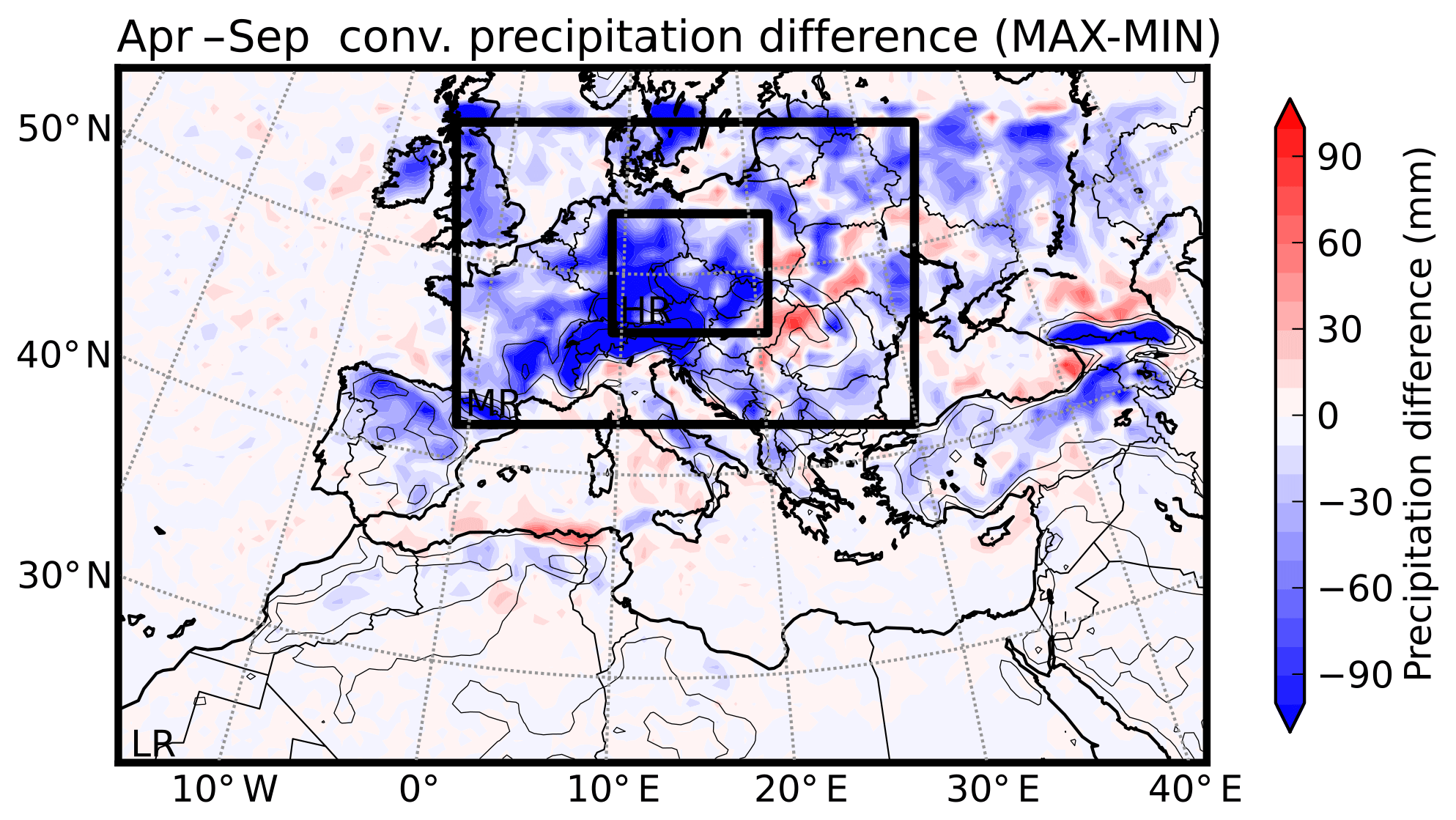
Figure 2Differences in convective precipitation between the MAX and the MIN simulations. The whole map is the LR simulation domain, the medium black box is the intermediate domain MR, and the small box is the HR domain.
The microphysical scheme used is the Thompson and Eidhammer (2014) scheme, which explicitly calculates the number concentrations of aerosols. The latter are represented in a simplified way according to their capacity to nucleate cloud water (“water-friendly” aerosols; WFAs) or ice water (“ice-friendly” aerosols; IFAs). Aerosol number concentrations are initialized and forced at domain boundaries by a climatology based on Goddard Chemistry Aerosol Radiation and Transport (GOCART) model (Ginoux et al., 2001) simulations. While no surface emissions are applied to IFAs, surface emission fluxes are applied to WFAs in order to approximately equilibrate the loss of WFAs due to scavenging and nucleation. The radiation scheme is RRTMG (rapid radiative transfer model for general circulation models; Iacono et al., 2008) and uses the cloud water droplets, ice, and snow effective radii of the Thompson and Eidhammer (2014) microphysical scheme to resolve the radiative transfer equations. Another climatology of aerosols from Tegen et al. (1997) is used in this radiative scheme and therefore is not affected by any changes in the microphysical aerosol climatology, which enables us to perform sensitivity experiments on the indirect effects of aerosols with a fixed aerosol direct effect. The Kain (2004) scheme is used to parameterize convection. The microphysical effects of aerosols are not taken into account explicitly in this parameterization, although they can affect convection indirectly through modifications in the temperature or moisture profiles.
This configuration is the same as in Da Silva et al. (2018), to which the reader is referred for additional detail.
2.2 Simulation experiments
The model was run to make two extreme simulations in terms of WFA and IFA microphysical concentrations. Both simulations start on 1 April 2013 (after 1 month of spin-up) and end on 17 September 2013. A very high aerosol emission level (1.75×10⁷ kg s−1 for the whole domain) is applied in the first simulation, referred to as MAX or polluted simulation, and a very low aerosol emission level ( kg s−1 for the whole domain) is applied for the other simulation, referred to as MIN or pristine simulation. Although these emission rates are extreme, maximal and minimal values permitted by the microphysics scheme reduce the range of variation of the number of WFAs (NWFAs) to between ∼10 and ∼10 000 cm−3, and of the number of IFAs (NIFAs) to between 0.005 and 10 000 cm−3. Therefore these latter extreme emission rates ensure that both the NIFAs and the NWFAs in the MIN (and MAX) simulation remain close to their minimal (and maximal) permitted values, which correspond to a factor of 2×10⁶ for the NIFAs and a factor of 103 for the NWFAs between the MAX and the MIN simulations. Such high differences in aerosol concentration between the two simulations ensure that aerosol indirect effects are strong enough to emerge from the potential noise between the MAX and the MIN simulations. On the flip side, extreme values of aerosol concentrations reach the bounds of permitted values in the microphysical scheme, suggesting that for these ranges of concentrations, the uncertainties associated with the parameterizations of microphysical processes may be more pronounced.
Another set of MIN and MAX simulations has been performed at a resolution at which convection is resolved (3.3 km) and in a smaller domain (HR domain) as seen in Fig. 2. An intermediate set of simulations was used to perform one-way nesting between the LR and the HR simulations, ensuring that the LR simulations force the HR simulations at their boundaries. These intermediate simulations were done at a resolution of 16.6 km in an intermediate domain (MR; see Fig. 2) and with the same configuration as the LR simulations. Under these conditions, each grid cell of the LR domain corresponds to exactly 15×15 grid cells of the HR domain. The HR simulations have been performed without activating any convection scheme since horizontal resolution (3.3 km) is sufficient to resolve convection processes, which is the only difference in model configuration between the LR simulations and the HR simulations. While the microphysical effects of aerosol on convective clouds were not taken into account due to the use of a convection scheme insensitive to aerosol concentrations, the whole set of indirect effects is represented in the HR simulations, including small-scale and large-scale processes.
2.3 Temperature–precipitation bin method
The simulation domain covers the Euro-Mediterranean region as displayed in Fig. 2. This figure also shows the difference in accumulated convective precipitation over the period of study between the MAX and the MIN simulations. It shows that most of the negative signal is concentrated over land regions where precipitation is more intense in this period of the year (Da Silva et al., 2018). The following analysis of convective precipitation reduction in the MAX simulation is conducted over the HR domain. Indeed, the location of the HR domain was chosen because of the high negative values of convective precipitation differences between the MAX and the MIN simulations in this area and because it is far away from oceanic areas where flux imbalance with the non-coupled oceanic surface may hinder interpretation as discussed in Da Silva et al. (2018). Because of the short duration of our simulations, temperature at the first vertical grid level (centred around 28 m above the ground; hereafter referred to as surface) and convective precipitation hourly time series were collected for all grid points of the WRF that were inside the HR domain and then concatenated. To avoid snow precipitation, we selected only the events with daily mean temperatures warmer than 5 ∘C.
The method used to scale precipitation with temperature is similar to the one used by Hardwick et al. (2010). Temperature has a diurnal variation and may be impacted by precipitation events. Since for each precipitation event we want the corresponding temperature that represents the air mass, the daily average temperature is used. We selected hours with strictly positive precipitation amount in both the MIN and MAX time series and placed the pairs of daily mean temperatures and hourly precipitation into eight bins of 5896 samples according to the daily temperatures. In each bin the 50th percentile of daily mean temperature, the 50th percentile of precipitation, and the 95th percentile of precipitation are used for our analysis.
We focus on the contributions of precipitation efficiency, surface water vapour mixing ratio, and maximum vertical wind speed to the difference of convective precipitation scaling with a temperature between the MAX and the MIN simulations. We define precipitation efficiency as the ratio between the total mass of condensate of a column and the effective rate of precipitation that reaches the surface. For the LR simulations, it is calculated using hourly output variables of the WRF and following the parameterization of Kain (2004) implemented in the model in which precipitation efficiency is a decreasing function of cloud base height and vertical wind shear. Because the model output frequency is lower than the typical convective characteristic time, we expect large uncertainties. Precipitation efficiency is not explicitly calculated in the HR simulations; we therefore estimated it using the ratio of precipitation divided by the product of maximum vertical wind speed and surface water mixing ratio. For the LR simulations, the maximum vertical wind speed is calculated using the square root of surface-based convective available potential energy (CAPE), which is more representative of convective vertical motions than the resolved vertical velocity. These three variables are computed 1 h before the convective precipitation occurrence to better represent the air inside the updraught of the convective cell rather than the air inside its downdraught.
The contribution of each variable to the change in precipitation between the MAX and MIN simulations is computed for both median and extreme precipitation events, which are defined as follows. Median events are all events in which precipitation is between the 40th and the 60th percentile in at least one of the simulations (MIN or MAX). Extreme events are all events beyond the 90th percentile in at least one of the simulations (MIN or MAX). Median and extreme events are sorted as a function of the corresponding daily mean temperature and placed in eight bins with the same number of events per bin. For median or extreme precipitation, the median daily mean temperature is paired with each of the four variables (precipitation, precipitation efficiency, surface water vapour mixing ratio, and maximum vertical wind speed along the atmospheric column) in the MIN and the MAX simulations.
3.1 Sensitivity of temperature–precipitation scaling to change in aerosol loads
Figure 3 displays the 50th (panels a, c) and 95th (panels b, d) percentiles of hourly convective (panels a, b) and total (panels c, d) precipitation as a function of daily mean temperature at the surface for both the LR MIN (magenta) and the LR MAX (blue) simulations. Median total precipitation displays a negative scaling with surface temperature for both LR and HR simulations (Fig. 4a). Since the temperature range is spread over two seasons, it is likely that changes in large-scale forcings between spring and summer events may explain the decrease in median precipitation with surface temperature. Sub-CC scaling for median total precipitation is consistent with the study of Hardwick et al. (2010) in Australia. On the other hand, median convective precipitation follows a nearly CC scaling in our LR simulations, indicating that, unlike median total precipitation events, convective precipitation events seem to be mostly affected by changes in surface temperature rather than changes in large-scale dynamics.
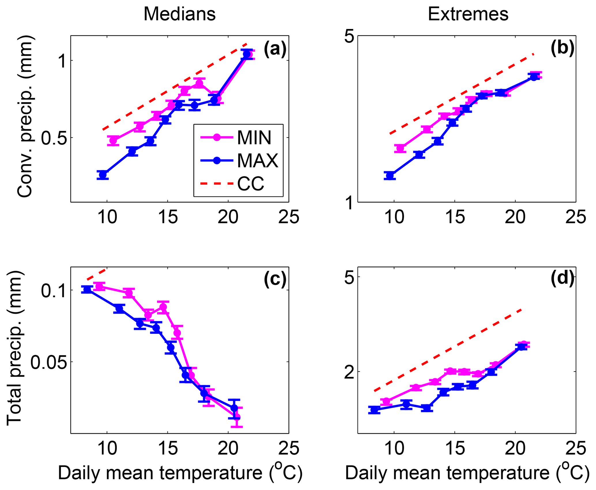
Figure 3Hourly convective (a, b) and total (c, d) precipitation as a function of daily mean temperature at the surface for median (a, c) and extreme (95th percentile; b, d) precipitation and for both the LR MIN (magenta) and LR MAX (blue) simulations. The dashed red line indicates the CC slope calculated using the August–Magnus–Roche approximation for saturated vapour pressure (Alduchov and Eskridge, 1996). Error bars represent the 95 % confidence interval of the precipitation percentiles.

Figure 4Hourly total precipitation as a function of daily mean temperature at the surface for median (a) and extreme (95th percentile; b) precipitation and for both the HR MIN (magenta) and HR MAX (blue) simulations. The dashed red line indicates the CC slope calculated using the August–Magnus–Roche approximation for saturated vapour pressure. Error bars represent the 95 % confidence interval of the precipitation percentiles.
Regarding convective precipitation extremes, a nearly CC scaling appears in the LR simulation. Using in situ measurements in Switzerland, Molnar et al. (2015) found a scaling of 8.9 % ∘C−1 of hourly convective precipitation as a function of daily mean temperature. Lower but similar slopes are obtained in our study with a value of 6.1 % ∘C−1 for the LR MIN simulation and a value of 8.6 % ∘C−1 in the LR MAX simulation. Berg and Haerter (2013) and Loriaux et al. (2013) showed that the scaling between total extreme precipitation and daily mean temperature could be super-CC because of the distribution of convective and stratiform precipitation with respect to daily mean temperature. Convective precipitation is generally more intense and occurs at higher temperatures. Supposing that both convective and stratiform precipitation follow CC scaling, they argued that total precipitation will display a super-CC scaling for temperatures corresponding to the transition between stratiform and convective precipitation. Such an effect does not appear in our study since we can observe a slight sub-CC scaling for total extreme precipitation. The scaling of total extreme precipitation is therefore different from the hook shape found in the Drobinski et al. (2018) study in the Mediterranean area. As expected (Li et al., 2011), precipitation extremes are increased in the HR simulations with respect to the LR simulations. However, the slopes of the HR simulations are rather similar to the slopes of total precipitation in the LR simulations.
Differences between the MAX and the MIN simulations are similar for both extremes and medians in the HR and LR simulations. We find that convective precipitation is reduced in the MAX simulation, but only at low temperatures. This temperature dependency slightly changes the scaling between the MAX and the MIN simulations, with higher slopes in the MAX simulation (around 8.5 % ∘C−1 in LR) compared to the MIN simulation (around 6.2 % ∘C−1 in LR). The fact that indirect effects of aerosols are weaker at high temperatures is probably due to the lower occurrence of clouds under these conditions. Figure 5 shows the mean COD calculated as in Da Silva et al. (2018), as a function of daily mean temperature for both the MIN and MAX simulations for low and high resolutions. It shows a decrease in COD with temperatures in all of the simulations. When averaging over hours with a strictly positive COD, we found that the optical thickness of clouds is relatively constant over the temperature range (not shown), confirming that the decrease in COD with temperature is mostly due to a decrease in the occurrence of clouds with temperature. This tendency maximizes the indirect effects of aerosols at low temperatures and minimizes them at high temperatures. In their study of the impact of the microphysical scheme on the scaling of precipitation extremes with temperature, Singh and O'Gorman (2014) have also shown that the main effect occurs at low temperatures. They attributed the change in slope at low temperatures to a difference in the parameterization of hydrometeor fall speed. They argued that slower hydrometeor fall speed decreases precipitation efficiency through enhanced evaporation and detrainment and through reduced precipitation rate. In our case, convective precipitation is diagnosed with the same convective scheme in the LR MAX and LR MIN simulations, which takes into account neither aerosol concentration nor rain fall speed. Such a microphysical effect is therefore impossible for the LR simulations. In the HR simulations, however, convective precipitation is diagnosed by the microphysical scheme, which does represent the terminal fall speed of hydrometeors that may be different depending on the aerosol concentration, as found in other studies (Koren et al., 2015; Dagan et al., 2018). This effect is one among others that possibly acts to change the precipitation efficiency between the HR MAX and the HR MIN simulations. The next section is dedicated to evaluating how strong these changes in precipitation efficiency are relative to the background radiative effect between the MIN and the MAX simulations.
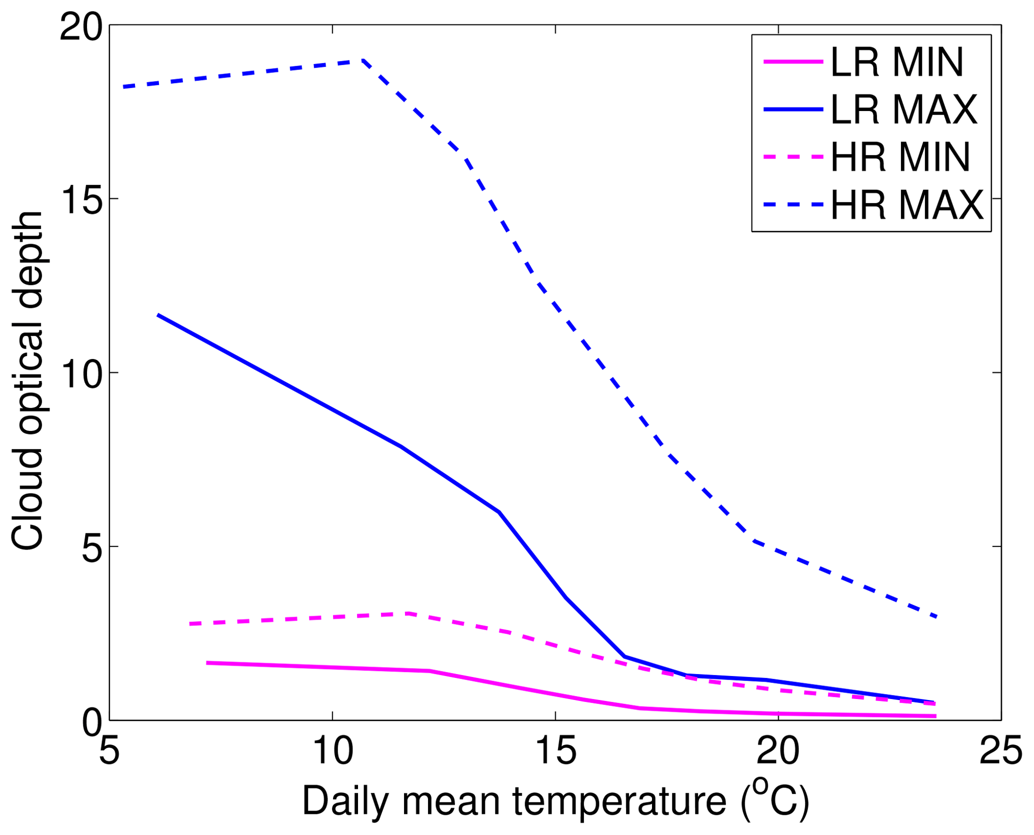
Figure 5Hourly COD as a function of daily mean temperature for the LR MIN (full magenta line), LR MAX (dashed blue line), HR MIN (dashed magenta line), and HR MAX (dashed blue line) simulations.
3.2 Process analysis
To analyse the reduction in convective precipitation at low temperatures, we consider that precipitation can be approximately described by the following equation (Drobinski et al., 2016; Da Silva, 2018):
with ε corresponding to the precipitation efficiency, Q the water vapour mixing ratio at the surface, and W the maximum vertical wind speed. This description is mostly valid for convective precipitation which results from a parcel that raises from the surface (Da Silva et al., 2018). Assuming the small changes in precipitation that we observe between the MAX and the MIN simulations, one can write
Figure 6 displays relative changes in convective precipitation vertical wind speed, precipitation efficiency, and the surface water vapour mixing ratio between the LR MAX and LR MIN simulations for median and extreme precipitation. As expected from Fig. 5, the decrease in convective precipitation in the MAX simulation with respect to the MIN simulation tends to be weaker with increasing temperature, from −25 % at 10 ∘C to almost 0 % at 22 ∘C. Among the three factors that may impact the precipitation intensity, the vertical velocity seems to explain much of the reduction in convective precipitation. Indeed, among the 25 % of precipitation reduction at low temperatures, around 15 % is attributable to the weakening of vertical velocity in the MAX simulation. It is also striking in Fig. 6 that the variations in the difference of vertical velocity and of convective precipitation with temperature are perfectly similar, with stronger reductions for low temperatures than for higher ones, while both precipitation efficiency and the surface water vapour mixing ratio display insignificant or erratic variations with temperature. Indeed, the high variations in precipitation efficiency differences with temperature for precipitation extremes may not reflect a physical process but only the difficulty in retrieving precipitation efficiency from hourly outputs.
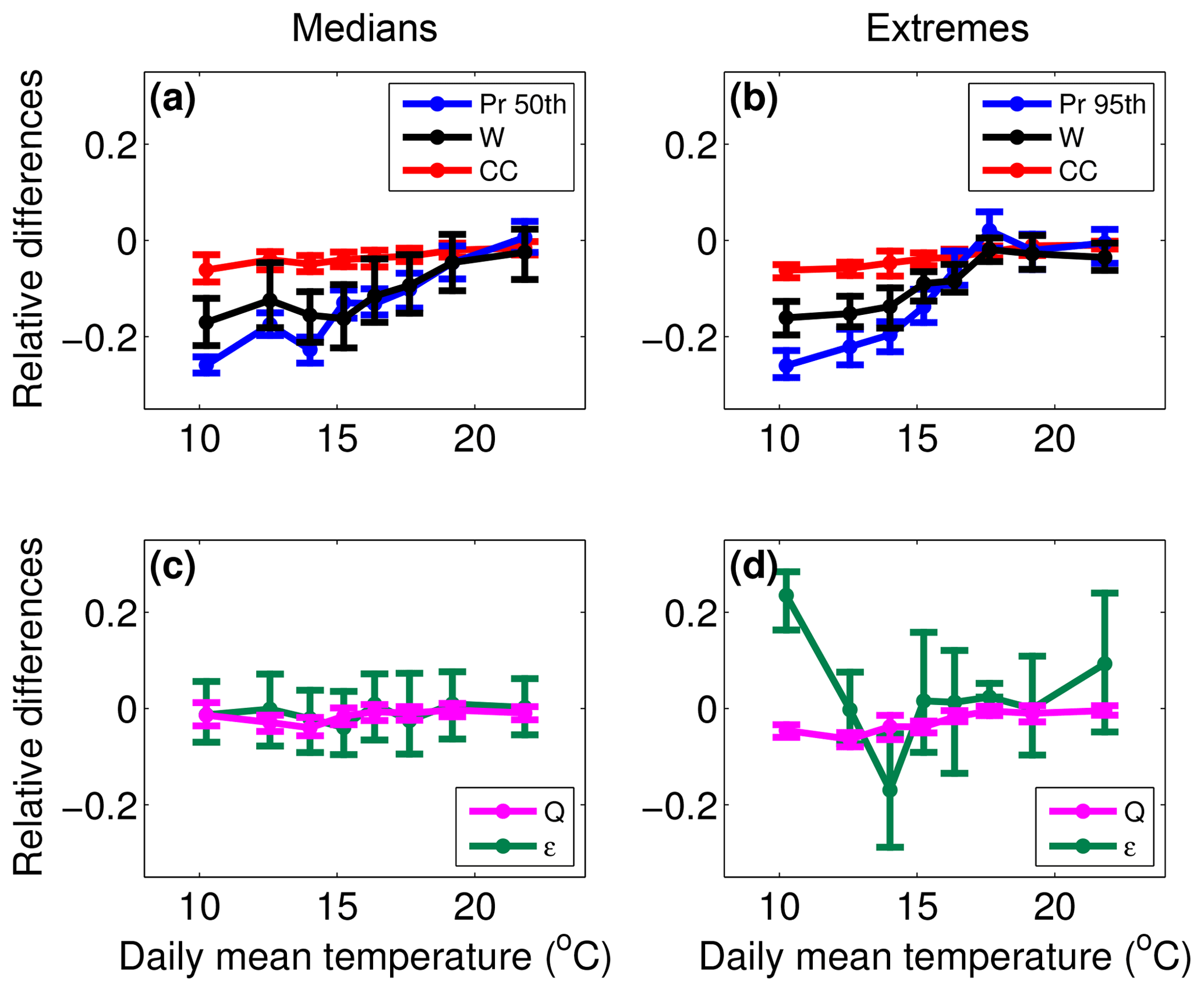
Figure 6Relative differences between LR MAX and LR MIN simulations of convective precipitation (blue, a, b), vertical velocity (black, a, b), surface water vapour mixing ratio (magenta, c, d), and precipitation efficiency (green, c, d) for median (a, c) and extreme (b, d) convective precipitation events as a function of the mean between the MIN and MAX daily mean temperature. The change expected according to the Clausius–Clapeyron law is displayed in red (a, b). Error bars represent the 95 % confidence interval of the precipitation percentiles.
The fact that vertical velocity drives the changes in convective precipitation explains why CC scaling is completely inaccurate for predicting changes in convective precipitation by indirect effects. In fact, even the differences in the surface water vapour mixing ratio between the MAX and MIN simulations do not exactly follow a CC scaling due to increased relative humidity in the MAX simulation: while the CC law prediction is around −4 %, the reduction in the surface water vapour mixing ratio in the MAX simulation is often less significant. One would expect that the sub-CC scaling of surface water vapour mixing ratio differences would result in a sub-CC scaling of convective precipitation differences, but it is actually the reverse (super-CC scaling) because of stronger changes in vertical velocity. The results are similar for both extreme and median precipitation except for precipitation efficiency differences, which display small variations for median precipitation and erratic variations for extreme precipitation, which may not have a physical meaning. Indeed, differences in precipitation efficiency are constrained by the scaling of precipitation (Eq. 3) and thus are expected to be negligible compared to the changes in vertical velocity. In our LR simulations, precipitation efficiency is calculated as a decreasing function of cloud base height and vertical wind shear. The increased relative surface humidity in the LR MAX simulation compared to the LR MIN simulation therefore would acts to increase the precipitation efficiency of the polluted simulation. The contribution of the change in the vertical wind shear is less evident, and its high temporal and spatial variability (Markowski and Richardson, 2007) may explain errors in retrieving precipitation efficiency from hourly outputs.
Figure 7 is the same as Fig. 6 with the exception that it uses total HR precipitation. Although the differences in vertical velocity and the surface water vapour mixing ratio for median precipitation events have approximately the same behaviour as temperature in the HR simulation with respect to the LR simulation, MAX–MIN differences in the median of total HR precipitation are stronger than the differences of the median of LR convective precipitation. Such positive bias compared to LR convective precipitation differences may be expected since Da Silva et al. (2018) showed that stratiform precipitation is increased in the MAX simulation. In contrast, it was found that hourly extreme precipitation is dominated by convective events at high temperatures (Loriaux et al., 2013). The decomposition of precipitation as a product of a thermodynamics, dynamics, and microphysics term made in the present study is theoretically better adapted to convective precipitation than to stratiform precipitation (Da Silva, 2018) and thus is not efficient in explaining differences in total median precipitation. In our LR simulations, we found that convective precipitation dominates extreme total precipitation from 10 ∘C (not shown), thus for most of our temperature bins. Therefore, the scaling of precipitation used in the present study (Eq. 2) can be used for extreme total precipitation in the HR simulation. Differences in extreme total precipitation in the HR simulation are similar to the differences in extreme convective precipitation in the LR simulation and scale well with the differences in maximum vertical velocities.
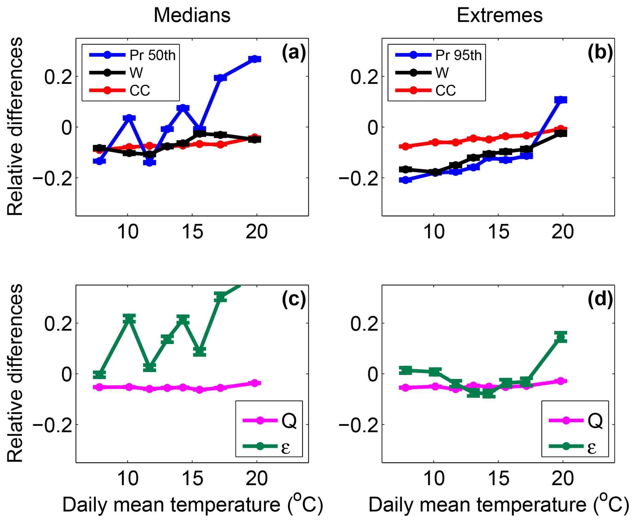
Figure 7Relative differences between HR MAX and HR MIN simulations of total precipitation (blue) and vertical velocity (black, a, b), precipitation efficiency (green, c, d), and surface water vapour mixing ratio (Q, magenta, c, d) for median (a, c) and extreme (b, d) precipitation events as a function of the mean between the MIN and MAX daily mean temperature. The change expected according to the Clausius–Clapeyron law is displayed in red (a, b). Error bars represent the 95 % confidence interval of the precipitation percentiles.
In this set of simulations with explicit convection, changes in aerosol concentration may have larger effects on convective precipitation efficiency since aerosols directly interact with convective clouds. Such impact has moreover been stated in many previous studies (Fan et al., 2009; Lebo and Seinfeld, 2011; Lebo and Morrison, 2014; Koren et al., 2015; Dagan et al., 2018; Miltenberger et al., 2018; Liu et al., 2019). The similarity of the precipitation differences with and without parameterized convection suggests that the changes in convective precipitation efficiency are relatively small in the HR simulation. Precipitation efficiency was calculated only indirectly since it is not parameterized for explicitly resolved precipitation. This was done by using the ratio of precipitation to the product of maximum vertical velocity and surface water vapour mixing ratio. Changes in precipitation efficiency between the MAX and the MIN simulations remain small in most of the temperature range. However, one can note a more significant increase in precipitation efficiency (around 15 %) in the warmest temperature bin, which is associated with increased precipitation extremes in the MAX simulation. The exact nature of increased precipitation efficiency only at the highest temperatures is not obvious and requires further investigations which are beyond the scope of the present study. The use of hourly outputs may also not be adapted to analyse these particular extreme events at high temperatures which were shown to be shorter than extreme precipitation events at lower temperatures (Utsumi et al., 2011; Drobinski et al., 2016; Gao et al., 2018).
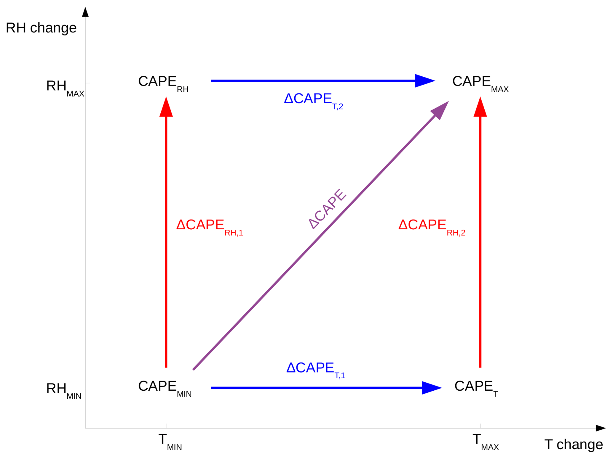
Figure 8Schematic of the two possible CAPE differences that permit us to evaluate the contribution of the vertical profile of temperature (ΔCAPET,1 and ΔCAPET,2) and the contribution of the vertical humidity profile (ΔCAPERH,1 and ΔCAPERH,2) to the change in total CAPE between the MAX and the MIN simulations (ΔCAPE).
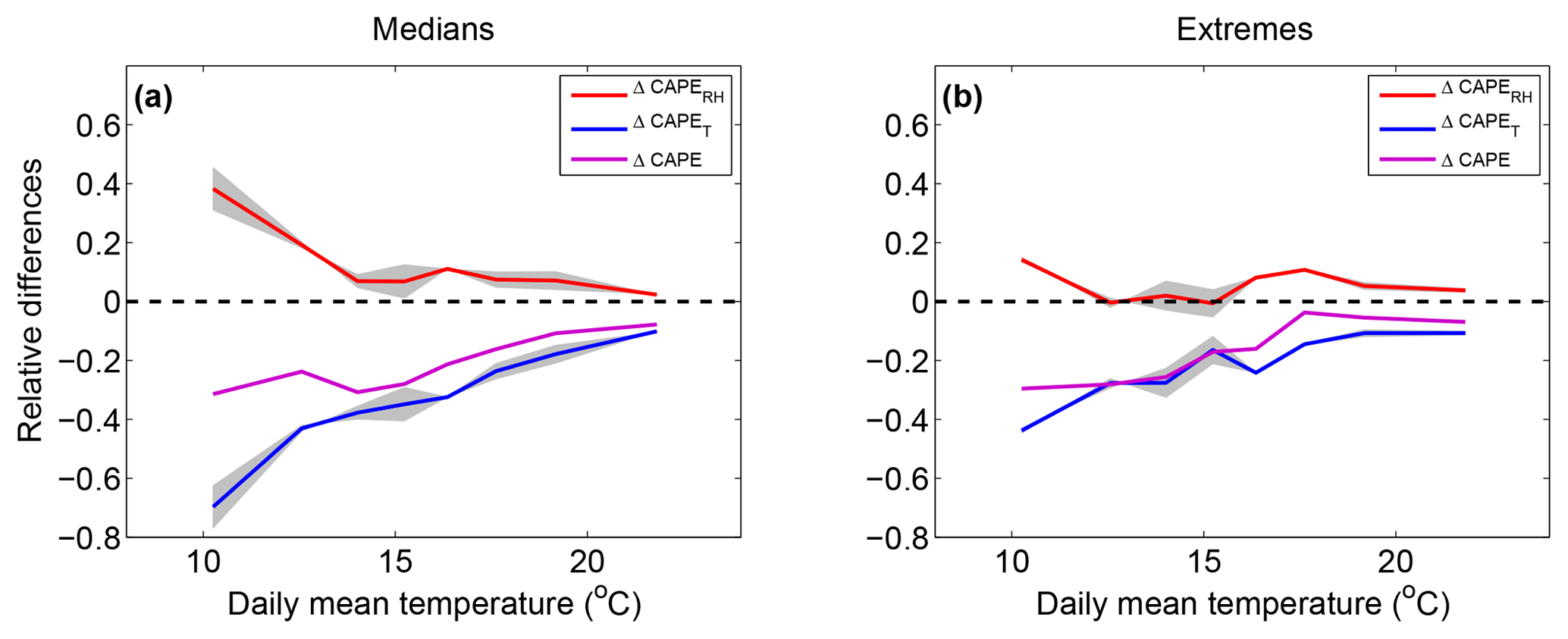
Figure 9Relative differences in CAPE between the LR MAX and the LR MIN simulations for median (a) and extreme (b) convective precipitation events (magenta, ΔCAPE). The temperature contribution (ΔCAPET) is displayed in blue and the relative humidity contribution (ΔCAPERH) in red.
3.3 Contributions of humidity and temperature to stability changes
As mentioned in Sect. 2.3, vertical velocity is calculated as the square root of CAPE. As seen in Fig. 1, CAPE may be affected by both surface temperature and surface humidity. CAPE is calculated using the entire profile of temperature and relative humidity (RH). Along these lines, we want to quantify the contribution of both the temperature and RH profile changes to the decrease in CAPE in the MAX simulation. For that purpose we have substituted the vertical profile of temperature in the MIN simulation with the vertical profile of temperature from the MAX simulation, and we have calculated two additional CAPEs, i.e. CAPET (and CAPERH) calculated with the temperature profile from the MAX (and MIN) simulation and the relative humidity from the MIN (and MAX) simulation, as represented in Fig. 8. Using the four CAPEs (CAPEMIN, CAPEMAX, CAPERH, and CAPET) we can compute relative differences (ΔCAPERH,1, ΔCAPERH,2, ΔCAPET,1, ΔCAPET,2, and ΔCAPE; see Fig. 8) and thus infer the contribution of temperature and RH vertical profiles to the change in CAPE between the MAX and the MIN simulations.
Figure 9 shows the total change in CAPE between the MAX and MIN simulations (ΔCAPE), the RH contribution , and the temperature contribution as a function of daily mean temperature for median and extreme precipitation events. The amount of CAPE is lower in the MAX simulation with respect to the MIN simulation, and ΔCAPE is more negative at low temperatures (−30 %) than at high temperatures (almost 0 %). However one can see that ΔCAPET and ΔCAPERH have opposite signs. Indeed, the RH contribution is positive and decreases from about +40 % at 10 ∘C to about 0 % at 22 ∘C for median precipitation events. The fact that this contribution is positive is not a surprise since we have seen in Fig. 6 that the surface RH is higher in the MAX simulation. We can see that this apparently weak increase in RH in the MAX simulation has a strong effect on the CAPE at low temperatures. However the main contribution is negative and comes from the differences in vertical temperature profiles: values range between −70 % at low temperatures and −15 % at high temperatures. Moreover, one can see similar variations in ΔCAPE and ΔCAPET with temperature.
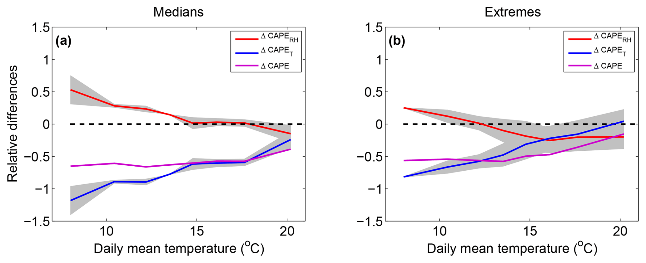
Figure 10Relative differences in CAPE between the HR MAX and HR MIN simulations for median (a) and extreme (b) precipitation events (magenta, ΔCAPE). The temperature vertical profile contribution (ΔCAPET) is displayed in blue and the relative humidity vertical profile contribution (ΔCAPERH) in red.
Figure 10 is the same as Fig. 9 but for the HR simulations and total precipitation. The amount of ΔCAPE is larger in the HR simulation, with values that exceed −50 % for a wide range of low temperatures in both median and extreme precipitation. These large values of ΔCAPE result in small negative differences in maximum vertical wind speed that do not exceed −10 % and are not correlated with total precipitation differences for median total precipitation events (see Fig. 7) because of the coexistence of convective and stratiform events. For extreme events, which mostly consist of convective events, the discrepancy between the strong changes in CAPE and the weaker changes in vertical velocities between the HR MAX and the HR MIN simulation may be explained by enhanced release of latent heat at the freezing level caused by increased vertical mass transport of water droplets in polluted conditions, as suggested by previous studies (Khain et al., 2004, 2005; Rosenfeld et al., 2008; Lebo and Seinfeld, 2011; Fan et al., 2013). Indeed, in the present study, CAPE is calculated using a simple formula that does not account for differences in the load of rising parcels as long as their temperature and their relative humidity remain unchanged. According to the theory described in Rosenfeld et al. (2008), the aerosol concentrations of our MAX simulation may, however, be too high for invigorating updraughts but would instead weaken them. The reduced changes in vertical velocity between our HR MAX and HR MIN simulations may therefore have another origin. It is also expected that the diffusion efficiency increases when increasing aerosol loading since the resulting increase in cloud drop number would lead to an increase in the total surface area of cloud droplets, enhancing condensation and latent heat release (Pinsky et al., 2012). However, our simulations were done using a saturation adjustment scheme, which excludes the possibility of increased cloud condensation (and its resulting stronger updraught) in the HR MAX simulation due to this process. Miltenberger et al. (2018) observed large increases in latent heating in the warm phase of clouds; these increases are thus not related to the theory of convective invigoration exposed in Rosenfeld et al. (2008). They attributed these changes to more organized cloud structures that limit dry air intrusions in the core of convective cells. Such an effect may also hold in our simulations since cloud cover and surface relative humidity are increased in the HR MAX simulation compared to the HR MIN simulation (not shown). According to the differences between the variations in CAPE and the variations in vertical velocities, this effect would limit the decrease in precipitation by about 10 % in the HR MAX simulation.
The contributions are otherwise similar to those of the LR simulations, with mainly a positive contribution of RH and a strongly negative contribution from the temperature vertical profile.
The amount of CAPE is a non-linear function of the temperature and humidity profiles. Therefore, the change ΔCAPET,1 is different from the change ΔCAPET,2. Similarly, the change ΔCAPERH,1 is different from the change ΔCAPERH,2. The quantities ΔCAPET,1 and ΔCAPET,2 (as well as ΔCAPERH,1 and ΔCAPERH,2) delimit a grey area in Fig. 9 that represents the uncertainty (relative to the non-linearity of CAPE) of the temperature (and RH) contribution. One can see that the effects of CAPE non-linearity are generally lower than the difference between each contribution. Where the grey areas do not intersect, i.e. in almost the entire temperature range for median precipitation, and for the cooler part of the distribution for extreme precipitation, a comparison of ΔCAPET, ΔCAPERH, and ΔCAPE strengthens the interpretation presented above: the negative value of ΔCAPE can be attributed to temperature changes, partially buffered by RH changes.
However the vertical temperature profile can be changed in several ways; e.g. one can only change the vertical gradient of temperature or uniformly reduce the temperature on the vertical. In the first configuration the decrease in CAPE would be purely due to the increase in stability of the environment, whereas in the second configuration the decrease in CAPE would be due to the surface air parcel temperature, more precisely to its reduced release of latent heat due to a reduction in its initial water vapour content.
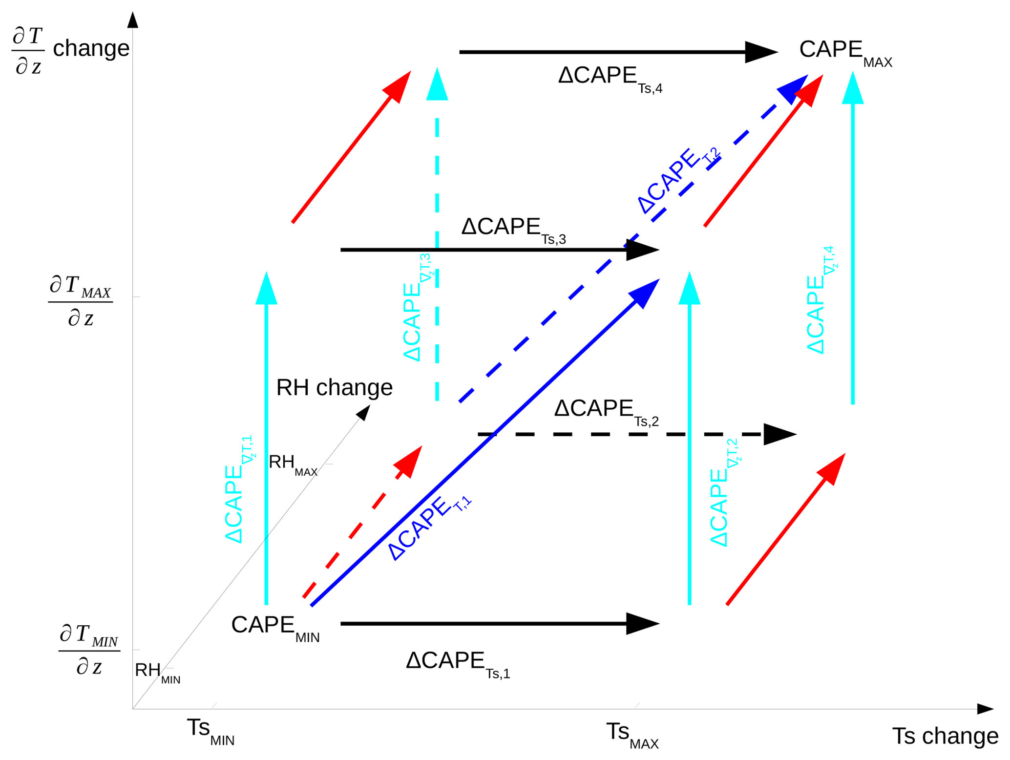
Figure 11Schematic of the four possible CAPE differences that permit us to evaluate the contribution of the vertical gradient of temperature (, , , and ) and the contribution of the surface temperature (, , , and ) to ΔCAPE.
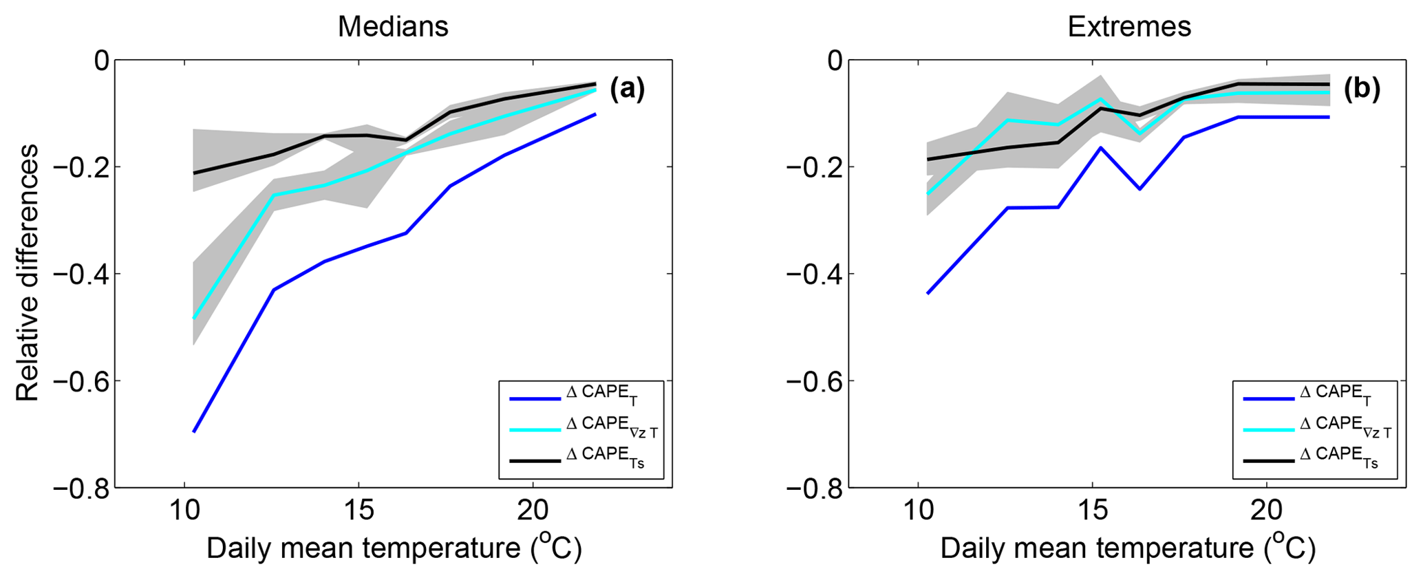
Figure 12Temperature vertical profile contribution to the change in CAPE between the LR MAX and the LR MIN simulation for median (a) and extreme (b) convective precipitation events (blue, ΔCAPET). The surface temperature contribution () is displayed in black and the temperature vertical gradient contribution () in cyan.
In this part, the temperature contribution is decomposed into two contributions: one from the vertical gradient of temperature and one from the surface temperature. The amount of CAPE can now be viewed as a function of three variables: the RH profile, the vertical temperature gradient, and the surface temperature. As displayed in Fig. 11, for a given RH profile (from the MIN or the MAX simulation), we have substituted the vertical temperature gradient (and surface temperature) from the MIN simulation with the vertical temperature gradient (and surface temperature) from the MAX simulation, and we have calculated four additional CAPEs using the four new mixed profiles. By calculating relative differences in CAPE, one can evaluate the contribution of the surface temperature and of the vertical gradient of temperature .
Figure 12 shows , , and ΔCAPET (as in Fig. 8) as a function of daily mean temperature for the LR simulations. The contribution of the vertical gradient of temperature and the contribution of the surface temperature are both negative, indicating not only that the surface temperature is lower in the MAX simulation but also that this cooling is less significant in the higher layers of the troposphere. Both processes tend to reduce the CAPE in the MAX simulation with respect to the MIN simulation. For median precipitation, the reduction in CAPE due to the vertical gradient of temperature (−10 % at high temperatures to −50 % at low temperatures) is more significant than the reduction in CAPE due to the surface temperature (−10 % at high temperatures to −20 % at low temperatures). For extreme precipitation, contributions are similar and range between −20 % at low temperatures to −5 % at high temperatures.
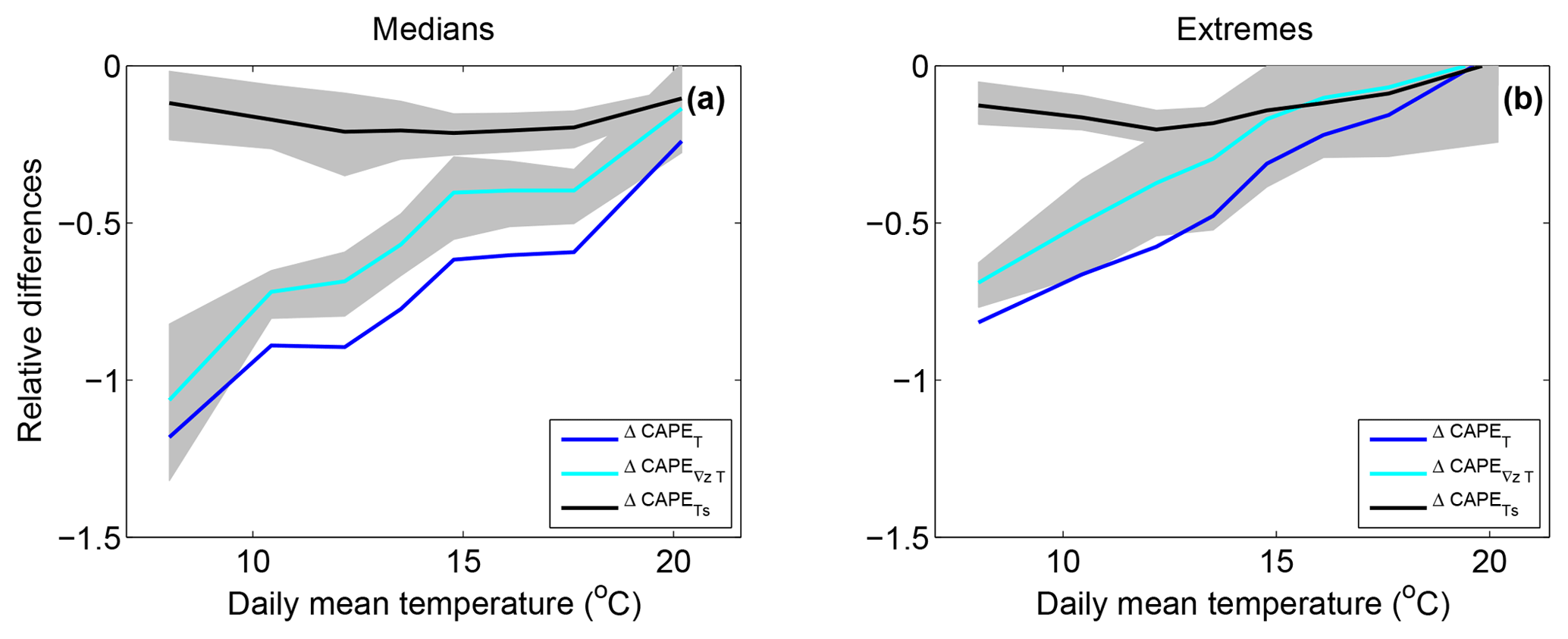
Figure 13Temperature vertical profile contribution to the change in CAPE between the HR MAX and the HR MIN simulation for median (a) and extreme (b) precipitation events (blue, ΔCAPET). The surface temperature contribution () is displayed in black and the temperature vertical gradient contribution () in cyan.
A similar analysis in the HR simulations is displayed in Fig. 13. The results are very similar to those from the LR simulations with the exception that for extreme precipitation with low temperatures, the temperature gradient contribution is significantly larger than the surface temperature contribution.
The maximum and the minimum values of (and ) delimit a grey area in Figs. 12 and 13 that represents the uncertainty related to the CAPE non-linearity. It shows that for both HR and LR simulations, the contributions are clearly different at low temperatures for median precipitation events, whereas the uncertainty ranges tend to overlap at high temperatures. For extreme events, the non-linearity of CAPE does not permit us to distinguish between the two contributions for the entire range of temperatures of the LR simulations. In the HR simulations, the non-linearity uncertainty is also too large at high temperatures to differentiate between the two contributions. However the contribution of the vertical gradient of temperature is significantly weaker than the contribution of the surface temperature at the lowest temperatures of the HR simulations.
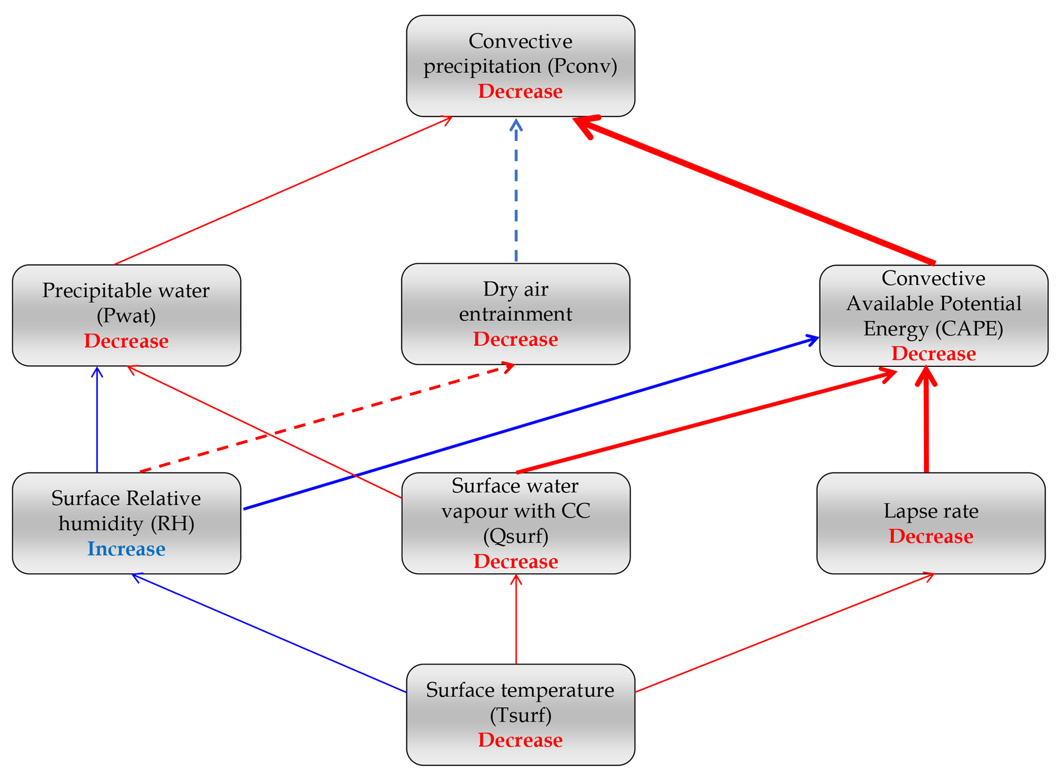
Figure 14Detailed schematic summary of the causal sequence that links the decrease in surface temperature to the decrease in convective precipitation in our polluted simulation. The size of the arrows gives a qualitative estimation of the contributions of each process. Dashed arrows indicate uncertain paths.
An evaluation of the processes involved in the reduction in convective precipitation by aerosol indirect effects is performed in the present study in the framework of the temperature–precipitation relationship. Figure 14 summarizes the various processes involved and their qualitative contribution (size of the arrows). The temperature–precipitation approach permits us to show that aerosol indirect effects on convective precipitation are larger at low temperatures than at high temperatures because clouds are statically more frequent and optically thicker at cool temperatures in our area of interest. Da Silva et al. (2018) found that convective precipitation is weakened in polluted environments through reduced atmospheric instability and water availability. With a simple decomposition of the decrease in convective precipitation in the polluted simulation, we show that this decrease is dominated by differences in atmospheric stability rather than differences in the moisture content of air parcels (Fig. 14). Therefore, the reduction in convective precipitation in the polluted simulation does not follow the Clausius–Clapeyron law: the simulated reduction in convective precipitation in a polluted environment compared to a pristine environment as determined in our simulations is actually stronger than the Clausius–Clapeyron scaling. Although taken into account in our simulations with explicit convection, the remaining aerosol indirect effects have only a relatively small impact on the precipitation efficiency of most of the extreme events in our simulations compared to the stability effect on convective updraughts. A noticeable increase in precipitation efficiency was, however, detected at the highest temperatures in the polluted simulation. The exact nature of the associated increase in precipitation extreme is beyond the scope of this study and requires further investigations.
Using the CAPE parameter as a measure of the atmospheric stability, we performed an in-depth analysis that estimates the contribution of each variable to the weakening of convective updraughts in the polluted simulation. Quantifying uncertainties related to the non-linearity of the CAPE is essential to correctly attribute the contribution of each variable to the stability modifications. Our method gives a first estimation of these uncertainties and shows that they are small enough to assess the following conclusions. The weakening of vertical velocity in convective updraughts is essentially explained by the stabilization of the vertical profile of temperature, which is partly compensated by an increase in relative humidity in the polluted simulation (Fig. 14). Our study also suggests the existence of a convective invigoration effect that also acts to compensate the stabilization in the HR simulations. The origin of the invigoration could be linked to reduced dry air intrusions in the convective cores of our polluted simulation, as hypothesized in the study of Miltenberger et al. (2018). The modification of the vertical temperature gradient, due to a stronger cooling in the boundary layer than in the free troposphere in the polluted simulation, is the most significant contribution for median precipitation events, whereas for extreme precipitation it is of similar magnitude as the contribution of the surface temperature decrease. Our simulations performed at high resolution are consistent with these results even though their interpretation is made more difficult by the fact that convective and stratiform precipitation are melted together while having opposite responses to aerosol indirect effects (as seen in Da Silva et al., 2018).
Due to the poor understanding of aerosol indirect effects (Fan et al., 2016) and the known uncertainties associated with numerical modelling (Crétat et al., 2012; Diaconescu et al., 2007; Flaounas et al., 2011; Foley, 2010; Ramarohetra et al., 2015; Seth and Giorgi, 1998), aerosol indirect effects have been found to be sensitive to the model configuration (Seifert and Beheng, 2006; Lebo and Seinfeld, 2011; Lebo et al., 2012; Fan et al., 2012; Morrison, 2012; Lebo and Morrison, 2014; Hill et al., 2015; Johnson et al., 2015; White et al., 2017; Heikenfeld et al., 2019). The results found with our specific model configuration are uncertain in this sense and need to be confirmed by further numerical and observational studies. It is also worth noting that these results were obtained using extremely low and extremely high aerosol concentrations. While this approach permits us to effectively retrieve the precipitation response to a drastic change in aerosol concentration, it is uncertain whether the magnitude of the involved processes does not change under less extreme aerosol conditions, as stated in other studies (Rosenfeld et al., 2008; Dagan et al., 2015; Miltenberger et al., 2018). Despite these limitations, our configuration highlights the importance of the background aerosol cloud radiative feedback and its repercussions on convective precipitation through changes in the thermodynamic profile of the atmosphere, which are often underestimated in case study simulations. It is suggested in this study that this effect might be higher than any convective invigoration effect, as predicted in Fan et al. (2013) using shorter simulations in a smaller domain. A more realistic estimation of the aerosol indirect effects on convective precipitation could be carried out with the use of online-coupled models in which aerosol concentration is evaluated with precise emission and transport schemes (Tuccella et al., 2019).
The WRF simulations used in this study can be obtained from the MISTRAL database website (registration required) at https://doi.org/10.14768/MISTRALS-HYMEX.1503 (Da Silva, 2019) or upon request to the authors.
PD, SM, and NDS designed the numerical experiments. NDS and SM performed the simulations. NDS prepared the manuscript with contributions from all co-authors.
The authors declare that they have no conflict of interest.
This article is part of the special issue “Hydrological cycle in the Mediterranean (ACP/AMT/GMD/HESS/NHESS/OS inter-journal SI)”. It is not associated with a conference.
This work is a contribution to the HyMeX project (HYdrological cycle in the Mediterranean EXperiment) as part of the INSU-MISTRALS programme. The authors are grateful to the editor and the two anonymous reviewers for their careful work and their valuable help in improving the manuscript.
This paper was edited by Philip Stier and reviewed by two anonymous referees.
Adler, R. F., Gu, G., Wang, J., Huffman, G. J., Curtis, S., and Bolvin, D.: Relationships between global precipitation and surface temperature on interannual and longer timescales (1979–2006), J. Geophys. Res.-Atmos., 113, D22104, https://doi.org/10.1029/2008JD010536, 2008. a
Albrecht, B.: Aerosols, cloud microphysics, and fractional cloudiness, Science, 245, 1227–1230, https://doi.org/10.1126/science.245.4923.1227, 1989. a
Alduchov, O. A. and Eskridge, R. E.: Improved Magnus Form Approximation of Saturation Vapor Pressure, J. Appl. Meteorol., 35, 601–609, https://doi.org/10.1175/1520-0450(1996)035<0601:IMFAOS>2.0.CO;2, 1996. a
Allen, M. R. and Ingram, W. J.: Constraints on future changes in climate and the hydrologic cycle, Nature, 419, 228–232, https://doi.org/10.1038/nature01092, 2002. a, b
Berg, P. and Haerter, J.: Unexpected increase in precipitation intensity with temperature — A result of mixing of precipitation types?, Atmos. Res., 119, 56–61, https://doi.org/10.1016/j.atmosres.2011.05.012, 2013. a, b
Boer, G. J.: Climate change and the regulation of the surface moisture and energy budgets, Clim. Dynam., 8, 225–239, https://doi.org/10.1007/BF00198617, 1993. a
Bollasina, M. A., Ming, Y., and Ramaswamy, V.: Anthropogenic Aerosols and the Weakening of the South Asian Summer Monsoon, Science, 334, 502–505, https://doi.org/10.1126/science.1204994, 2011. a, b
Crétat, J., Pohl, B., Richard, Y., and Drobinski, P.: Uncertainties in simulating regional climate of Southern Africa: sensitivity to physical parameterizations using WRF, Clim. Dynam., 38, 613–634, https://doi.org/10.1007/s00382-011-1055-8, 2012. a
Crhová, L. and Holtanová, E.: Simulated relationship between air temperature and precipitation over Europe: sensitivity to the choice of RCM and GCM, Int. J. Climatol., 38, 1595–1604, https://doi.org/10.1002/joc.5256, 2017. a
Dagan, G., Koren, I., and Altaratz, O.: Competition between core and periphery-based processes in warm convective clouds – from invigoration to suppression, Atmos. Chem. Phys., 15, 2749–2760, https://doi.org/10.5194/acp-15-2749-2015, 2015. a, b, c
Dagan, G., Koren, I., and Altaratz, O.: Quantifying the effect of aerosol on vertical velocity and effective terminal velocity in warm convective clouds, Atmos. Chem. Phys., 18, 6761–6769, https://doi.org/10.5194/acp-18-6761-2018, 2018. a, b
Da Silva, N.: Around the temperature-precipitation relationship in the Euro-Mediterranean region, Theses, Université Paris-Saclay, available at: https://pastel.archives-ouvertes.fr/tel-02059296, last access: December 2018. a, b
Da Silva, N.: Aerosol indirect effect sensitivities, ESPRI/IPSL, https://doi.org/10.14768/MISTRALS-HYMEX.1503, 2019. a
Da Silva, N., Mailler, S., and Drobinski, P.: Aerosol indirect effects on summer precipitation in a regional climate model for the Euro-Mediterranean region, Ann. Geophys., 36, 321–335, https://doi.org/10.5194/angeo-36-321-2018, 2018. a, b, c, d, e, f, g, h, i, j, k
Diaconescu, E. P., Laprise, R., and Sushama, L.: The impact of lateral boundary data errors on the simulated climate of a nested regional climate model, Clim. Dynam., 28, 333–350, https://doi.org/10.1007/s00382-006-0189-6, 2007. a
Drobinski, P., Ducrocq, V., Alpert, P., Anagnostou, E., Béranger, K., Borga, M., Braud, I., Chanzy, A., Davolio, S., Delrieu, G., Estournel, C., Boubrahmi, N. F., Font, J., Grubišić, V., Gualdi, S., Homar, V., Ivančan-Picek, B., Kottmeier, C., Kotroni, V., Lagouvardos, K., Lionello, P., Llasat, M. C., Ludwig, W., Lutoff, C., Mariotti, A., Richard, E., Romero, R., Rotunno, R., Roussot, O., Ruin, I., Somot, S., Taupier-Letage, I., Tintore, J., Uijlenhoet, R., and Wernli, H.: HyMeX: A 10-Year Multidisciplinary Program on the Mediterranean Water Cycle, B. Am. Meteorol. Soc., 95, 1063–1082, https://doi.org/10.1175/BAMS-D-12-00242.1, 2014. a
Drobinski, P., Alonzo, B., Bastin, S., Da Silva, N., and Muller, C.: Scaling of precipitation extremes with temperature in the French Mediterranean region: What explains the hook shape?, J. Geophys. Res.-Atmos., 121, 3100–3119, https://doi.org/10.1002/2015JD023497, 2016. a, b, c, d
Drobinski, P., Da Silva, N., Panthou, G., Bastin, S., Muller, C., Ahrens, B., Borga, M., Conte, D., Fosser, G., Giorgi, F., Güttler, I., Kotroni, V., Li, L., Morin, E., Önol, B., Quintana-Segui, P., Romera, R., and Torma, C. Z.: Scaling precipitation extremes with temperature in the Mediterranean: past climate assessment and projection in anthropogenic scenarios, Clim. Dynam., 51, 1237–1257, https://doi.org/10.1007/s00382-016-3083-x, 2018. a, b
Fan, J., Yuan, T., Comstock, J. M., Ghan, S., Khain, A., Leung, L. R., Li, Z., Martins, V. J., and Ovchinnikov, M.: Dominant role by vertical wind shear in regulating aerosol effects on deep convective clouds, J. Geophys. Res.-Atmos., 114, D22206, https://doi.org/10.1029/2009JD012352, 2009. a
Fan, J., Rosenfeld, D., Ding, Y., Leung, L. R., and Li, Z.: Potential aerosol indirect effects on atmospheric circulation and radiative forcing through deep convection, Geophys. Res. Lett., 39, L09806, https://doi.org/10.1029/2012GL051851, 2012. a
Fan, J., Leung, L. R., Rosenfeld, D., Chen, Q., Li, Z., Zhang, J., and Yan, H.: Microphysical effects determine macrophysical response for aerosol impacts on deep convective clouds, P. Natl. Acad. Sci. USA, 110, E4581–E4590, https://doi.org/10.1073/pnas.1316830110, 2013. a, b, c, d, e
Fan, J., Wang, Y., Rosenfeld, D., and Liu, X.: Review of Aerosol–Cloud Interactions: Mechanisms, Significance, and Challenges, J. Atmos. Sci., 73, 4221–4252, https://doi.org/10.1175/JAS-D-16-0037.1, 2016. a
Flaounas, E., Bastin, S., and Janicot, S.: Regional climate modelling of the 2006 West African monsoon: Sensitivity to convection and planetary boundary layer parameterisation using WRF, Clim. Dynam., 36, 1083–1105, https://doi.org/10.1007/s00382-010-0785-3, 2011. a
Foley, A.: Uncertainty in regional climate modelling: A review, Prog. Phys. Geog., 34, 647–670, https://doi.org/10.1177/0309133310375654, 2010. a
Gao, X., Zhu, Q., Yang, Z., Liu, J., Wang, H., Shao, W., and Huang, G.: Temperature Dependence of Hourly, Daily, and Event-based Precipitation Extremes Over China, Sci. Rep., 8, 17564–17564, https://doi.org/10.1038/s41598-018-35405-4, 2018. a
Ginoux, P., Chin, M., Tegen, I., Prospero, J. M., Holben, B., Dubovik, O., and Lin, S.-J.: Sources and distributions of dust aerosols simulated with the GOCART model, J. Geophys. Res.-Atmos., 106, 20255–20273, https://doi.org/10.1029/2000JD000053, 2001. a
Haerter, J. O. and Berg, P.: Unexpected rise in extreme precipitation caused by a shift in rain type?, Nat. Geosci., 2, 372–373, https://doi.org/10.1038/ngeo523, 2009. a
Hardwick, J. R., Westra, S., and Sharma, A.: Observed relationships between extreme sub-daily precipitation, surface temperature, and relative humidity, Geophys. Res. Lett., 37, L22805, https://doi.org/10.1029/2010GL045081, 2010. a, b, c, d
Heikenfeld, M., White, B., Labbouz, L., and Stier, P.: Aerosol effects on deep convection: the propagation of aerosol perturbations through convective cloud microphysics, Atmos. Chem. Phys., 19, 2601–2627, https://doi.org/10.5194/acp-19-2601-2019, 2019. a
Held, I. M. and Soden, B. J.: Robust Responses of the Hydrological Cycle to Global Warming, J. Climate, 19, 5686–5699, https://doi.org/10.1175/JCLI3990.1, 2006. a, b
Hill, A. A., Shipway, B. J., and Boutle, I. A.: How sensitive are aerosol-precipitation interactions to the warm rain representation?, J. Adv. Model. Earth Syst., 7, 987–1004, https://doi.org/10.1002/2014MS000422, 2015. a
Iacono, M. J., Delamere, J. S., Mlawer, E. J., Shephard, M. W., Clough, S. A., and Collins, W. D.: Radiative forcing by long-lived greenhouse gases: Calculations with the AER radiative transfer models, J. Geophys. Res.-Atmos., 113, D13103, https://doi.org/10.1029/2008JD009944, 2008. a
Johnson, J. S., Cui, Z., Lee, L. A., Gosling, J. P., Blyth, A. M., and Carslaw, K. S.: Evaluating uncertainty in convective cloud microphysics using statistical emulation, J. Adv. Model. Earth Syst., 7, 162–187, https://doi.org/10.1002/2014MS000383, 2015. a
Kain, J. S.: The Kain–Fritsch Convective Parameterization: An Update, J. Appl. Meteorol., 43, 170–181, https://doi.org/10.1175/1520-0450(2004)043<0170:TKCPAU>2.0.CO;2, 2004. a, b
Khain, A. and Lynn, B.: Simulation of a supercell storm in clean and dirty atmosphere using weather research and forecast model with spectral bin microphysics, J. Geophys. Res.-Atmos., 114, D19209, https://doi.org/10.1029/2009JD011827, 2009. a
Khain, A., Pokrovsky, A., Pinsky, M., Seifert, A., and Phillips, V.: Simulation of Effects of Atmospheric Aerosols on Deep Turbulent Convective Clouds Using a Spectral Microphysics Mixed-Phase Cumulus Cloud Model. Part I: Model Description and Possible Applications, J. Atmos. Sci., 61, 2963–2982, https://doi.org/10.1175/JAS-3350.1, 2004. a, b, c
Khain, A., Rosenfeld, D., and Pokrovsky, A.: Aerosol impact on the dynamics and microphysics of deep convective clouds, Q. J. Roy. Meteor. Soc., 131, 2639–2663, https://doi.org/10.1256/qj.04.62, 2005. a, b, c
Koren, I., Altaratz, O., and Dagan, G.: Aerosol effect on the mobility of cloud droplets, Environ. Res. Lett., 10, 104011, https://doi.org/10.1088/1748-9326/10/10/104011, 2015. a, b
Lebo, Z. J.: The Sensitivity of a Numerically Simulated Idealized Squall Line to the Vertical Distribution of Aerosols, J. Atmos. Sci., 71, 4581–4596, https://doi.org/10.1175/JAS-D-14-0068.1, 2014. a
Lebo, Z. J. and Morrison, H.: Dynamical Effects of Aerosol Perturbations on Simulated Idealized Squall Lines, Mon. Weather Rev., 142, 991–1009, https://doi.org/10.1175/MWR-D-13-00156.1, 2014. a, b, c
Lebo, Z. J. and Seinfeld, J. H.: Theoretical basis for convective invigoration due to increased aerosol concentration, Atmos. Chem. Phys., 11, 5407–5429, https://doi.org/10.5194/acp-11-5407-2011, 2011. a, b, c, d, e
Lebo, Z. J., Morrison, H., and Seinfeld, J. H.: Are simulated aerosol-induced effects on deep convective clouds strongly dependent on saturation adjustment?, Atmos. Chem. Phys., 12, 9941–9964, https://doi.org/10.5194/acp-12-9941-2012, 2012. a
Lelieveld, J., Berresheim, H., and Borrmann, S.: Global air pollution crossroads over the Mediterranean, Science, 298, 794–799, https://doi.org/10.1126/science.1075457, 2002. a
Lenderink, G. and van Meijgaard, E.: Increase in hourly precipitation extremes beyond expectations from temperature changes, Nat. Geosci., 1, 511–514, https://doi.org/10.1038/ngeo262, 2008. a
Lenderink, G., Barbero, R., Loriaux, J. M., and Fowler, H. J.: Super-Clausius–Clapeyron Scaling of Extreme Hourly Convective Precipitation and Its Relation to Large-Scale Atmospheric Conditions, J. Climate, 30, 6037–6052, https://doi.org/10.1175/JCLI-D-16-0808.1, 2017. a
Li, F., Collins, W. D., Wehner, M. F., Williamson, D. L., Olson, J. G., and Algieri, C.: Impact of horizontal resolution on simulation of precipitation extremes in an aqua-planet version of Community Atmospheric Model (CAM3), Tellus A, 63, 884–892, 2011. a
Liu, H., Guo, J., Koren, I., Altaratz, O., Dagan, G., Wang, Y., Jiang, J. H., Zhai, P., and Yung, Y. L.: Non-Monotonic Aerosol Effect on Precipitation in Convective Clouds over Tropical Oceans, Sci. Rep., 9, 7809–7809, https://doi.org/10.1038/s41598-019-44284-2, 2019. a, b
Loriaux, J. M., Lenderink, G., De Roode, S. R., and Siebesma, A. P.: Understanding Convective Extreme Precipitation Scaling Using Observations and an Entraining Plume Model, J. Atmos. Sci., 70, 3641–3655, https://doi.org/10.1175/JAS-D-12-0317.1, 2013. a, b
Madden, R. A. and Williams, J.: The correlation between temperature and precipitation in the United States and Europe, Mon. Weather Rev., 106, 142–147, https://doi.org/10.1175/1520-0493(1978)106<0142:TCBTAP>2.0.CO;2, 1978. a
Malavelle, F. F., Haywood, J. M., Jones, A., Gettelman, A., Clarisse, L., Bauduin, S., Allan, R. P., Karset, I. H. H., Kristjánsson, J. E., Oreopoulos, L., Cho, N., Lee, D., Bellouin, N., Boucher, O., Grosvenor, D. P., Carslaw, K. S., Dhomse, S., Mann, G. W., Schmidt, A., Coe, H., Hartley, M. E., Dalvi, M., Hill, A. A., Johnson, B. T., Johnson, C. E., Knight, J. R., O'Connor, F. M., Partridge, D. G., Stier, P., Myhre, G., Platnick, S., Stephens, G. L., Takahashi, H., and Thordarson, T.: Strong constraints on aerosol-cloud interactions from volcanic eruptions, Nature, 546, 485–491, https://doi.org/10.1038/nature22974, 2017. a
Markowski, P. and Richardson, Y.: Observations of Vertical Wind Shear Heterogeneity in Convective Boundary Layers, Mon. Weather Rev., 135, 843–861, https://doi.org/10.1175/MWR3334.1, 2007. a
Miltenberger, A. K., Field, P. R., Hill, A. A., Rosenberg, P., Shipway, B. J., Wilkinson, J. M., Scovell, R., and Blyth, A. M.: Aerosol–cloud interactions in mixed-phase convective clouds – Part 1: Aerosol perturbations, Atmos. Chem. Phys., 18, 3119–3145, https://doi.org/10.5194/acp-18-3119-2018, 2018. a, b, c, d, e, f, g
Molnar, P., Fatichi, S., Gaál, L., Szolgay, J., and Burlando, P.: Storm type effects on super Clausius–Clapeyron scaling of intense rainstorm properties with air temperature, Hydrol. Earth Syst. Sci., 19, 1753–1766, https://doi.org/10.5194/hess-19-1753-2015, 2015. a, b
Morrison, H.: On the robustness of aerosol effects on an idealized supercell storm simulated with a cloud system-resolving model, Atmos. Chem. Phys., 12, 7689–7705, https://doi.org/10.5194/acp-12-7689-2012, 2012. a
Morrison, H. and Grabowski, W. W.: Cloud-system resolving model simulations of aerosol indirect effects on tropical deep convection and its thermodynamic environment, Atmos. Chem. Phys., 11, 10503–10523, https://doi.org/10.5194/acp-11-10503-2011, 2011. a, b
Muller, C.: Impact of Convective Organization on the Response of Tropical Precipitation Extremes to Warming, J. Climate, 26, 5028–5043, https://doi.org/10.1175/JCLI-D-12-00655.1, 2013. a, b
Muller, C. J. and O'Gorman, P. A.: An energetic perspective on the regional response of precipitation to climate change, Nat. Clim. Change, 1, 266–271, https://doi.org/10.1038/nclimate1169, 2011. a
Muller, C. J., O’Gorman, P. A., and Back, L. E.: Intensification of Precipitation Extremes with Warming in a Cloud-Resolving Model, J. Climate, 24, 2784–2800, https://doi.org/10.1175/2011JCLI3876.1, 2011. a
National Centers for Environmental Prediction/National Weather Service/NOAA/U.S. Department of Commerce: NCEP FNL Operational Model Global Tropospheric Analyses, continuing from July 1999. Research Data Archive at the National Center for Atmospheric Research, Computational and Information Systems Laboratory, updated daily, https://doi.org/10.5065/D6M043C6, 2000. a
Omrani, H., Drobinski, P., and Dubos, T.: Optimal nudging strategies in regional climate modelling: investigation in a Big-Brother experiment over the European and Mediterranean regions, Clim. Dynam., 41, 2451–2470, https://doi.org/10.1007/s00382-012-1615-6, 2013. a
Omrani, H., Drobinski, P., and Dubos, T.: Using nudging to improve global-regional dynamic consistency in limited-area climate modeling: What should we nudge?, Clim. Dynam., 44, 1627–1644, https://doi.org/10.1007/s00382-014-2453-5, 2015. a
Pall, P., Allen, M. R., and Stone, D. A.: Testing the Clausius–Clapeyron constraint on changes in extreme precipitation under CO2 warming, Clim. Dynam., 28, 351–363, https://doi.org/10.1007/s00382-006-0180-2, 2007. a
Panthou, G., Mailhot, A., Laurence, E., and Talbot, G.: Relationship between Surface Temperature and Extreme Rainfalls: A Multi-Time-Scale and Event-Based Analysis, J. Hydrometeorol., 15, 1999–2011, https://doi.org/10.1175/JHM-D-14-0020.1, 2014. a, b
Pinsky, M., Khain, A., Mazin, I., and Korolev, A.: Analytical estimation of droplet concentration at cloud base, J. Geophys. Res.-Atmos., 117, https://doi.org/10.1029/2012JD017753, 2012. a
Ramanathan, V., Crutzen, P. J., Kiehl, J. T., and Rosenfeld, D.: Aerosols, Climate, and the Hydrological Cycle, Science, 294, 2119–2124, https://doi.org/10.1126/science.1064034, 2001. a
Ramarohetra, J., Pohl, B., and Sultan, B.: Errors and uncertainties introduced by a regional climate model in climate impact assessments: example of crop yield simulations in West Africa, Environ. Res. Lett., 10, 124014, https://doi.org/10.1088/1748-9326/10/12/124014, 2015. a
Rodrigo, F. S.: Coherent variability between seasonal temperatures and rainfalls in the Iberian Peninsula, 1951–2016, Theor. Appl. Climatol., 135, 473–490, https://doi.org/10.1007/s00704-018-2400-1, 2019. a
Rosenfeld, D., Lohmann, U., Raga, G. B., O’Dowd, C. D., Kulmala, M., Fuzzi, S., Reissell, A., and Andreae, M. O.: Flood or Drought: How Do Aerosols Affect Precipitation?, Science, 321, 1309–1313, https://doi.org/10.1126/science.1160606, 2008. a, b, c, d, e
Salameh, T., Drobinski, P., and Dubos, T.: The effect of indiscriminate nudging time on large and small scales in regional climate modelling: Application to the Mediterranean basin, Q. J. Roy. Meteor. Soc., 136, 170–182, https://doi.org/10.1002/qj.518, 2010. a
Salzmann, M., Weser, H., and Cherian, R.: Robust response of Asian summer monsoon to anthropogenic aerosols in CMIP5 models, J. Geophys. Res.-Atmos., 119, 11321–11337, https://doi.org/10.1002/2014JD021783, 2014. a, b
Seifert, A. and Beheng, K. D.: A two-moment cloud microphysics parameterization for mixed-phase clouds. Part 2: Maritime vs. continental deep convective storms, Meteorol. Atmos. Phys., 92, 67–82, https://doi.org/10.1007/s00703-005-0113-3, 2006. a
Seifert, A., Heus, T., Pincus, R., and Stevens, B.: Large-eddy simulation of the transient and near-equilibrium behavior of precipitating shallow convection, J. Adv. Model. Earth Syst., 7, 1918–1937, https://doi.org/10.1002/2015MS000489, 2015. a
Seth, A. and Giorgi, F.: The effects of domain choice on summer precipitation simulation and sensitivity in a regional climate model, J. Climate, 11, 2698–2712, 1998. a
Singh, M. S. and O'Gorman, P. A.: Influence of microphysics on the scaling of precipitation extremes with temperature, Geophys. Res. Lett., 41, 6037–6044, https://doi.org/10.1002/2014GL061222, 2014. a
Singleton, A. and Toumi, R.: Super-Clausius–Clapeyron scaling of rainfall in a model squall line, Q. J. Roy. Meteor. Soc., 139, 334–339, https://doi.org/10.1002/qj.1919, 2013. a
Skamarock, W., Klemp, J., Dudhia, J., Gill, D., Barker, D., Wang, W., Huang, X.-Y., Duda, M., and Powers, J.: A Description of the Advanced Research WRF Version 3, NCAR Tech. Note NCAR/TN-475+STR, https://doi.org/10.5065/D68S4MVH, 113 pp., 2008. a
Small, J. D., Chuang, P. Y., Feingold, G., and Jiang, H.: Can aerosol decrease cloud lifetime?, Geophys. Res. Lett., 36, L16806, https://doi.org/10.1029/2009GL038888, 2009. a
Stevens, B. and Feingold, G.: Untangling aerosol effects on clouds and precipitation in a buffered system, Nature, 461, 607–613, https://doi.org/10.1038/nature08281, 2009. a
Stjern, C. W., Samset, B. H., Myhre, G., Forster, P. M., Hodnebrog, ., Andrews, T., Boucher, O., Faluvegi, G., Iversen, T., Kasoar, M., Kharin, V., Kirkevåg, A., Lamarque, J.-F., Olivié, D., Richardson, T., Shawki, D., Shindell, D., Smith, C. J., Takemura, T., and Voulgarakis, A.: Rapid adjustments cause weak surface temperature response to increased black carbon concentrations, J. Geophys. Res.-Atmos., 122, 11462–11481, https://doi.org/10.1002/2017JD027326, 2017. a
Tegen, I., Hollrig, P., Chin, M., Fung, I., Jacob, D., and Penner, J.: Contribution of different aerosol species to the global aerosol extinction optical thickness: Estimates from model results, J. Geophys. Res.-Atmos., 102, 23895–23915, https://doi.org/10.1029/97JD01864, 1997. a
Thompson, G. and Eidhammer, T.: A Study of Aerosol Impacts on Clouds and Precipitation Development in a Large Winter Cyclone, J. Atmos. Sci., 71, 3636–3658, https://doi.org/10.1175/JAS-D-13-0305.1, 2014. a, b
Trenberth, K. E.: Atmospheric Moisture Residence Times and Cycling: Implications for Rainfall Rates and Climate Change, Climatic Change, 39, 667–694, https://doi.org/10.1023/A:1005319109110, 1998. a
Trenberth, K. E. and Shea, D. J.: Relationships between precipitation and surface temperature, Geophys. Res. Lett., 32, L14703, https://doi.org/10.1029/2005GL022760, 2005. a
Tuccella, P., Menut, L., Briant, R., Deroubaix, A., Khvorostyanov, D., Mailler, S., Siour, G., and Turquety, S.: Implementation of Aerosol-Cloud Interaction within WRF-CHIMERE Online Coupled Model: Evaluation and Investigation of the Indirect Radiative Effect from Anthropogenic Emission Reduction on the Benelux Union, Atmosphere, 10, 20, https://doi.org/10.3390/atmos10010020, 2019. a
Twomey, S.: The Influence of Pollution on the Shortwave Albedo of Clouds, J. Atmos. Sci., 34, 1149–1152, https://doi.org/10.1175/1520-0469(1977)034<1149:TIOPOT>2.0.CO;2, 1977. a
Utsumi, N., Seto, S., Kanae, S., Maeda, E. E., and Oki, T.: Does higher surface temperature intensify extreme precipitation?, Geophys. Res. Lett., 38, L16708, https://doi.org/10.1029/2011GL048426, 2011. a, b
White, B., Gryspeerdt, E., Stier, P., Morrison, H., Thompson, G., and Kipling, Z.: Uncertainty from the choice of microphysics scheme in convection-permitting models significantly exceeds aerosol effects, Atmos. Chem. Phys., 17, 12145–12175, https://doi.org/10.5194/acp-17-12145-2017, 2017. a
Xue, H. and Feingold, G.: Large-Eddy Simulations of Trade Wind Cumuli: Investigation of Aerosol Indirect Effects, J. Atmos. Sci., 63, 1605–1622, https://doi.org/10.1175/JAS3706.1, 2006. a
Zhao, W. and Khalil, M. A. K.: The Relationship between Precipitation and Temperature over the Contiguous United States, J. Climate, 6, 1232–1236, https://doi.org/10.1175/1520-0442(1993)006<1232:TRBPAT>2.0.CO;2, 1993. a
Zhou, C. and Penner, J. E.: Why do general circulation models overestimate the aerosol cloud lifetime effect? A case study comparing CAM5 and a CRM, Atmos. Chem. Phys., 17, 21–29, https://doi.org/10.5194/acp-17-21-2017, 2017. a