the Creative Commons Attribution 4.0 License.
the Creative Commons Attribution 4.0 License.
 | 15 May 2020
Simulating age of air and the distribution of SF6 in the stratosphere with the SILAM model
Rostislav Kouznetsov
Mikhail Sofiev
Julius Vira
Gabriele Stiller
The paper presents a comparative study of age of air (AoA) derived from several approaches: a widely used passive-tracer accumulation method, the SF6 accumulation, and a direct calculation of an ideal-age tracer. The simulations were performed with the Eulerian chemistry transport model SILAM driven with the ERA-Interim reanalysis for 1980–2018.
The Eulerian environment allowed for simultaneous application of several approaches within the same simulation and interpretation of the obtained differences. A series of sensitivity simulations revealed the role of the vertical profile of turbulent diffusion in the stratosphere, destruction of SF6 in the mesosphere, and the effect of gravitational separation of gases with strongly different molar masses.
The simulations reproduced well the main features of the SF6 distribution in the atmosphere observed by the MIPAS (Michelson Interferometer for Passive Atmospheric Sounding) satellite instrument. It was shown that the apparent very old air in the upper stratosphere derived from the SF6 profile observations is a result of destruction and gravitational separation of this gas in the upper stratosphere and the mesosphere. These processes make the apparent SF6 AoA in the stratosphere several years older than the ideal-age AoA, which, according to our calculations, does not exceed 6–6.5 years. The destruction of SF6 and the varying rate of emission make SF6 unsuitable for reliably deriving AoA or its trends. However, observations of SF6 provide a very useful dataset for validation of the stratospheric circulation in a model with the properly implemented SF6 loss.
- Article
(8958 KB) - Full-text XML
- BibTeX
- EndNote


The age of air (AoA) is defined as the time spent by an air parcel in the stratosphere since its entry across the tropopause (Li and Waugh, 1999; Waugh and Hall, 2002). The distribution of the AoA is controlled by the global atmospheric circulations, primarily the Brewer–Dobson and polar circulations. In particular, the temporal variation of AoA has been used as an indicator of the long-term changes in the stratospheric circulation (Engel et al., 2009; Waugh, 2009). AoA has been extensively used for evaluation and comparison of general circulation and chemical transport models in the stratosphere (Waugh and Hall, 2002; Engel et al., 2009).
Simulations of the AoA as defined above have been performed with Lagrangian transport models. The trajectories are initiated with positions distributed in the stratosphere and integrated backwards in time until they cross the tropopause. The time elapsed since the initialization is attributed as age of air at the point of initialization. Moreover, the distribution of the ages of particles originating from some location can be used to get the age spectrum there. Until recently, Lagrangian simulations of AoA did not explicitly account for turbulent mixing in the stratosphere (Eluszkiewicz et al., 2000; Waugh and Hall, 2002; Diallo et al., 2012; Monge-Sanz et al., 2012). Accounting for mixing adds up to 2 years to the mean AoA in the tropical upper stratosphere (Garny et al., 2014). In Lagrangian models, the mixing can be simulated with random-walk of the particles (Garny et al., 2014) or by inter-parcel mixing (Plöger et al., 2015; Brinkop and Jöckel, 2019).
The Eulerian simulations of AoA can be formulated in several ways. The approaches with an accumulating tracer, whose mixing ratio increases linearly in the troposphere, were used in a comprehensive study by Krol et al. (2018) and several studies before (e.g. Eluszkiewicz et al., 2000; Monge-Sanz et al., 2012). Another approach is to simulate a steady distribution of a decaying tracer, such as 221Rn, emitted at the surface at a constant rate (Krol et al., 2018). Besides that, a special tracer that is analogous to the Lagrangian clock has been used. The tracer appears in the literature under names such as “clock-type tracer” (Monge-Sanz et al., 2012) or “ideal age” (Waugh and Hall, 2002). The ideal age has a constant rate of increasing of mixing ratio everywhere, except for the surface where it is continuously forced to zero. Similar tracers have long been used to simulate the transport times of oceanic water (e.g. England, 1995; Thiele and Sarmiento, 1990).
Direct observations of the age of air, as it is defined above, are not possible; therefore, AoA is usually derived from the observed mixing ratios of various tracers with known tropospheric mixing ratios and lifetimes (Bhandari et al., 1966; Koch and Rind, 1998; Jacob et al., 1997; Patra et al., 2011) or from the long-living tracers with known variations in the tropospheric mixing ratios. The studies published to date used carbon dioxide (CO2; Andrews et al., 2001; Engel et al., 2009), nitrous oxide (N2O; Boering et al., 1996; Andrews et al., 2001), sulfur hexafluoride (SF6; Waugh, 2009; Stiller et al., 2012), methane (CH4; Andrews et al., 2001; Remsberg, 2015), and various fluorocarbons (Leedham Elvidge et al., 2018).
For accumulating tracers, the mean AoA at some point in the stratosphere is calculated as a lag between the times when a certain mixing ratio is observed near the surface and at that point. The lag time is equivalent to the mean AoA defined above only in the case of the strictly linear growth and the uniform distribution of the tracer in the troposphere (Hall and Plumb, 1994).
In reality, there is no tracer whose mixing ratio in the troposphere grows strictly linearly. The violation of the assumption of the linear growth leads to biases in the resulting AoA distribution and its trends. It has been pointed out that the increasing growth rates of CO2 and SF6 lead to a low bias of AoA and its trends and make these tracers ambiguous proxies of the AoA (Garcia et al., 2011). Various corrections have been applied in several studies (Hall and Plumb, 1994; Waugh and Hall, 2002; Engel et al., 2009; Stiller et al., 2012; Leedham Elvidge et al., 2018) to deduce the “true” AoA from observations of tracers with the increasing growth rates. The effect of the correction method on the AoA estimates has not been investigated and must be considered a source of uncertainty in the resulting estimates. Thus, Garcia et al. (2011) concluded that accounting for the biases in the trend estimates due to varying growth rates would likely require uniform and continuous knowledge of the evolution of the trace species, which is not available from any existing observational dataset. Recently Leedham Elvidge et al. (2018) showed a minor sensitivity of the AoA to the choice of the correction method but without detailed analysis of the assumptions behind these methods. For a similar problem with the ages of oceanic water, it has been shown (Waugh et al., 2003) that, in the case of a inhomogeneously growing tracer, the tracer age is strongly influenced by the shape of the transient time distribution (TTD, also known as the “age spectrum”) at the particular location and time.
Another major source of uncertainty in the observational AoA is the violation of conservation of the tracer due to sources and sinks, such as oxidation of carbon monoxide and methane for CO2 or mesospheric destruction for SF6. The mesospheric sink of SF6 leads to “over-ageing”, especially pronounced in the area of the polar vortices. The magnitude of the over-ageing was estimated to be as at least 2 years (Waugh and Hall, 2002). Besides being visible in many evaluations, e.g. Stiller et al. (2012, Fig. 4) and Kovács et al. (2017, Fig. 8), the over-ageing of the polar winter stratospheric air was studied by Ray et al. (2017, Fig. 4) within the dedicated exercise.
The simulations of SF6 and the AoA in the atmosphere with the WACCM model (Kovács et al., 2017) have also reproduced the effect of over-ageing. However, its magnitude was much smaller than that inferred from the SF6 retrievals of the limb-viewing MIPAS (Michelson Interferometer for Passive Atmospheric Sounding) instrument operated on board of the Envisat satellite in 2002–2012 (Stiller et al., 2012) and from the in situ observations of the ER-2 aircraft (Hall et al., 1999). Kovács et al. (2017) offered two possible reasons for the discrepancy: either SF6 loss is still underestimated in WACCM or MIPAS SF6 observations are low biased above ∼20 km. Neither of the cases have been analysed in depth, which leaves the status of MIPAS, currently the richest observational dataset for the stratospheric SF6, unclear.
The aim of the present study is to provide self-consistent simulations of the spatio-temporal distribution of the AoA and of the SF6 mixing ratio in the troposphere and the stratosphere during the last 39 years. The main modelling tool is the Eulerian chemistry transport model SILAM (System for Integrated modeLling of Atmospheric coMposition). The stratospheric balloon observations and retrievals of the limb-viewing MIPAS instrument mentioned above are used for validation of the simulated distribution.
With these simulations we
-
compare different methods of estimating the AoA and quantify the inconsistencies in the AoA and its trends arising from violations of the underlying assumptions behind each method,
-
analyse the causes of the discrepancies in the upper stratosphere between different methods of deriving the AoA,
-
provide a solid basis for further studies of stratospheric circulation with observations of various trace gases and for studies of climate effects of SF6.
The paper is organized as follows. Section 2 gives an overview of the modelling tools and the modelling and observational data used for the study. Section 3 describes the developments made for SILAM in order to perform the simulations: vertical eddy-diffusivity parameterization in the stratosphere and the lower mesosphere and the SF6 destruction parametrization, as well as the model configuration used for the study. The sensitivity tests and evaluation of the simulations against the MIPAS retrievals and stratospheric balloon measurements of SF6 mixing ratios are given in Sect. 4. Sensitivity of the AoA and its trends to the simulation setup and the choice of particular SF6 tracer as an AoA proxy is studied in Sect. 5. The uncertainties of the used modelling approach and implications of AoA derived from SF6 tracer are discussed in Sect. 6. The results are summarized in Sect. 7.
2.1 SILAM model
SILAM (System for Integrated modeLling of Atmospheric coMposition, http://silam.fmi.fi, last access: 13 May 2020) is an offline 3D chemical transport model. SILAM features a mass-conservative positive-definite advection scheme that makes the model suitable for long-term runs (Sofiev et al., 2015). The model can be run at a range of resolutions starting from a kilometre scale in a limited-area up to a global coverage. The vertical structure of the modelling domain consists of stacked layers starting from the surface. The layers can be defined either in z- or hybrid sigma-pressure coordinates. The model can be driven with a variety of NWP (numerical weather prediction) or climate models.
The global 3D simulations of atmospheric transport for a variety of tracers representing AoA and SF6 (see Sect. 3.4 for details) were performed with SILAM for the years 1980–2018 with the global long–lat grid of cells (250×123 grid cells plus polar closures) and 60 hybrid sigma-pressure layers starting from the surface. The uppermost layer was between pressures of 0.1 and 0.2 hPa, whereas other layer bounds corresponded to the half levels of the meteorological driver – the ERA-Interim reanalysis (Sect. 2.2). The model time step was 15 min and the output consisted of daily-mean 3D concentrations of the tracers and air density. Emission data were taken from the SF6 emission inventory (Rigby et al., 2010), which was extrapolated until 2016 as described in Sect. 3.4. Physical–chemical transformations of the SF6-related tracers required developments described in Sect. 3.3.
In order to accurately model the AoA and the needed tracers, the vertical diffusion part of the transport scheme of SILAM has been refined to account for gravitational separation. In addition, several tracers with corresponding transformation routines have been implemented into the model. The SILAM configuration, used for the present study, is described in Sect. 3.4.
2.2 ECMWF ERA-Interim reanalysis
The ERA-Interim reanalysis of the European Centre for Medium-Range Weather Forecasts (ECMWF) had been used as a meteorological driver for our simulations. The dataset has T255 spectral resolution and covers the whole atmosphere with 60 hybrid sigma-pressure levels having the uppermost layer from 0.2 to 0 hPa with nominal pressure of 0.2 hPa (Dee et al., 2011). The reanalysis uses a 12 h data assimilation cycle, and the forecasts are stored with a 3 h time step. We used the fields retrieved from the ECMWF's MARS archive on a long–lat grid, 500×250 points, with a step of 0.72∘. The four forecast times (+3, +6, +9 and +12 h) were used from every assimilation cycle to obtain a continuous dataset with 3 h time step. To drive the dispersion model, the data on horizontal winds, temperature, and humidity for 1980–2018 were used.
Since the resolution of the driving meteorology was twice higher than that of SILAM, the meteorological input for both cell interface for winds and cell mid-points for other parameters (surface pressure, temperature, and humidity) was available without interpolation. The gridded ERA-Interim fields are, however, a result of reprojection of the original meteorological fields computed as spherical harmonics. Moreover, the difference in the topmost layer of the ERA-Interim and SILAM data required vertical reprojection at the top of the domain. Together with the limited precision of the gridded fields retrieved from the ECMWF archive, they caused some inconsistency between the surface-pressure tendencies and the vertically integrated air-mass fluxes calculated from the meteorological fields in SILAM. Albeit small, such inconsistencies cause spurious variations in wind-field divergence that might result in gradual accumulation of errors in the tracer mixing ratios. To maintain strict global and local air-mass budget throughout the run, the wind fields were adjusted by distributing the residuals of pressure tendency and vertically integrated horizontal air-mass fluxes as a correction to the horizontal winds, as suggested by Heimann and Keeling (1989). The correction was, at most, of the order of centimetres per second, which is comparable to the precision of the input wind fields. The vertical wind component was then rediagnosed from the divergence of the horizontal air-mass fluxes for the SILAM layers as described in Sofiev et al. (2015). Validity of this procedure was demonstrated by its authors Heimann and Keeling (1989) and its applicability to the current case was confirmed in the Sect. 5.2 by comparison with another model simulations driven by ERA-Interim (Diallo et al., 2012).
The ERA-Interim reanalysis has been used earlier for Lagrangian simulations of AoA (Diallo et al., 2012) and has been found to provide ages that agree with those inferred from in situ observations in the lower stratosphere.
2.3 MIPAS observations of SF6
To evaluate the results of the SF6 modelling, we used the data from the MIPAS instrument operated on board Envisat in 2002–2012. MIPAS is a limb-sounding Fourier transform spectrometer with a high spectral resolution measuring in the infrared part of spectrum. Due to its limb geometry, the instrument provided good vertical resolution of the derived trace-gas profiles and showed high sensitivity to low-abundance species around the tangent point. Along the orbit path, MIPAS measured a profile of atmospheric radiances about every 400 km with an altitude coverage, in its nominal mode, from 6 to 70 km. The vertical sampling was 1.5 km in the lower part of the stratosphere (up to 32 km) and 3 km above, with a vertical field of view covering 3 km at the tangent point. Over a day, about 1300 profiles along 14.4 orbits were measured, covering all latitudes up to the poles at sunlit and dark conditions. The vertical distributions of trace gases were derived from the radiance profiles by an inversion procedure, fitting simulated spectra to the measured ones while varying the atmospheric state parameters.
The retrieval of SF6 is based on the spectral signature of this species in the vicinity of 10.55 µm wavelength and is described in Stiller et al. (2008), Stiller et al. (2012), and Haenel et al. (2015). In the current study, we use an updated version of the SF6 data (compared to the one described in Haenel et al., 2015) called V5H/R_SF6_21/224/225. The new algorithm uses the new absorption cross-section data on the SF6 and a new CFC-11 band in the vicinity of the SF6 signature by Harrison (2018) instead of the older cross-section data by Varanasi et al. (1994). The updated version provides up to 0.6 pmol mol−1 higher SF6 mixing ratios in the upper part of the stratosphere (above 30 km) than the old versions and is closer to independent reference data. Note that whilst we regard this newer version of MIPAS SF6 data as an improvement, it has not yet been reported in a publication, and on that basis it is subject to uncertainty.
The retrieved profiles are sampled on an altitude grid spaced at 1 km, whereas the actual resolution of the profiles is between 4 and 10 km for altitudes below 30 km. The retrievals are supplemented with averaging kernels and error covariance matrices describing the uncertainties due to random noise in the radiance measurements, hereinafter referred to as measurement noise error, target noise error, or retrieval noise error. This error component, which is normally of the order of 10 % of the retrieved value, is fully uncorrelated from profile to profile, and therefore it virtually cancels out when averaged over a large number of profiles. In contrast, there exist systematic error components that are fully correlated between the profiles. Their assessment is difficult and depends on the knowledge about sources of systematic errors. Stiller et al. (2008) has assessed them to be of the order of 10 % at 60 km and 4 % at 30 km. These error components have to be considered when comparisons of monthly or seasonal means with other data are performed.
Destruction of atmospheric SF6 occurs at altitudes above 60 km (Totterdill et al., 2015) that fall within the topmost layer of the ERA-Interim data. The exchange processes in the upper stratosphere and lower mesosphere have to be adequately parameterized together with the destruction process. In our simulations we have suppressed the transport of SF6 with mean wind through the modelling domain top (0.1 hPa, 65 km) and parameterized the SF6 loss due to the eddy and molecular diffusion towards the altitudes where the destruction occurs. In this section we introduce the set of parameterizations that were implemented in SILAM for this study.
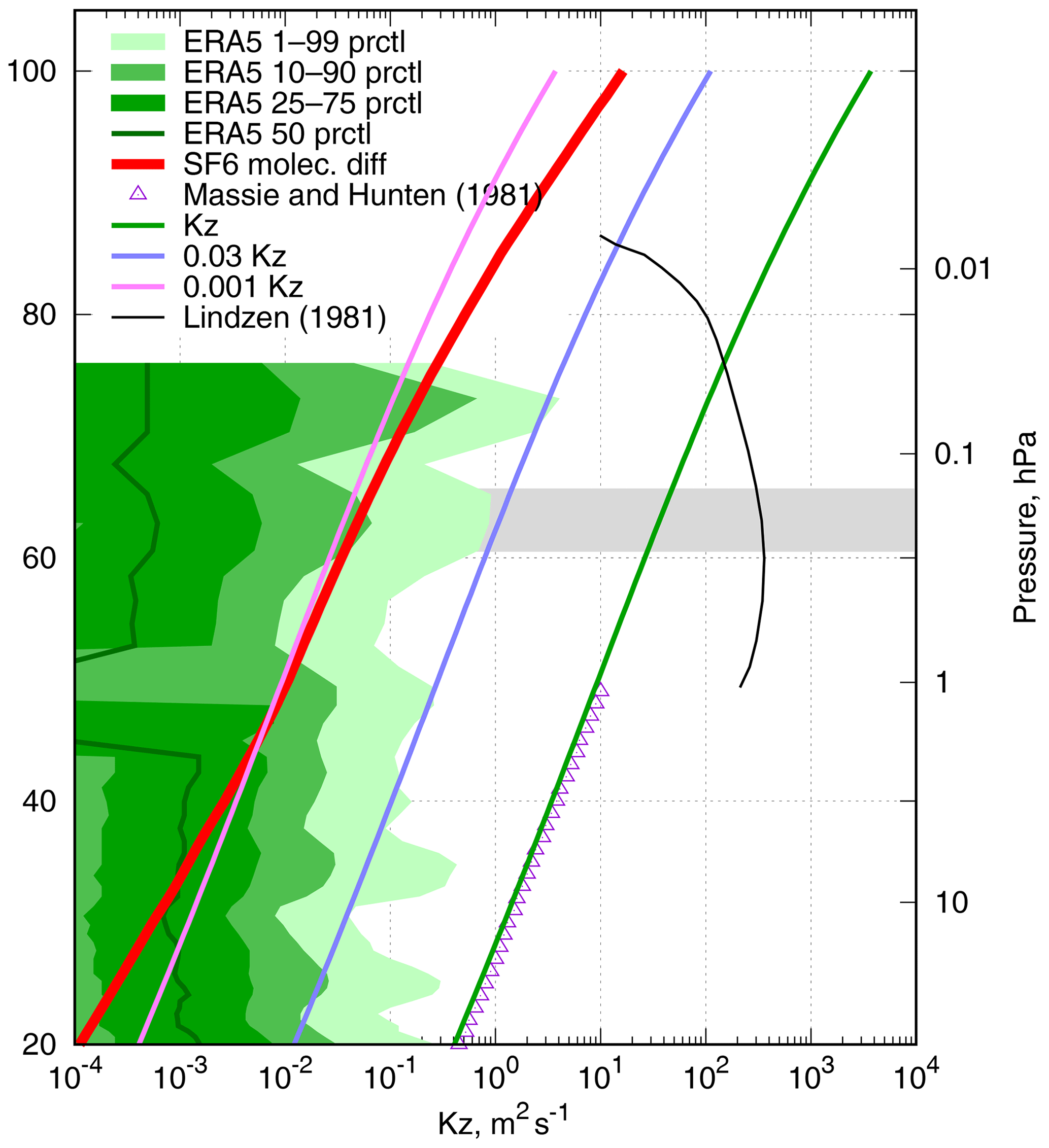
Figure 1Vertical profiles of diffusion coefficients are shown. The distribution of the ERA5 profiles of the “mean turbulent diffusion coefficient for heat” parameter, molecular diffusivity for SF6 in the U.S. Standard Atmosphere, and the three prescribed Kz profiles are shown. The eddy diffusion profile due to breaking gravity waves (after Lindzen, 1981) is given for the reference.
3.1 Eddy diffusivity
A large variety of vertical profiles for eddy diffusivity in the stratosphere and the lower mesosphere can be found in literature. In many studies in the 1970s–1980s, the vertical profiles were derived from observed tracer concentrations neglecting the mean transport. Most studies suggested that the vertical eddy diffusion has a minimum of 0.2–0.5 m2 s−1 (Pisso and Legras, 2008) at 15–20 km, agreeing quite well to the ones derived from the radar measurements in the range of 15–20 km (Wilson, 2004). Above that altitude, Kz was suggested to gradually increase by about 1.5 orders of magnitude towards 50 km due to breaking gravity waves (Lindzen, 1981).
The theoretical estimates of the effective exchange coefficients, considering the layered and patchy structure of stratospheric turbulence, suggest 0.5–2.5 m2 s−1 for the upper troposphere and 0.015–0.02 m2 s−1 for the lower stratosphere (Osman et al., 2016), which is about an order of magnitude lower than the estimates above.
The values of the eddy exchange coefficient at heights of 10–20 km estimated from the high-resolution balloon temperature measurements (Gavrilov et al., 2005) are ∼0.01 m2 s−1 with no noticeable vertical variation. It is not clear, however, how representative the derived values are for UTLS (upper troposphere and lower stratosphere) in general. We could not find any reliable observations of vertical diffusion in a range of 30–50 km.
The parameterization for vertical eddy diffusivity above the boundary layer used in SILAM has been adapted from the IFS model of the European Centre for Medium-Range Weather Forecasts (ECMWF, 2015). However, in the upper troposphere the predicted eddy diffusivity is nearly zero. For numerical reasons, a lower limit of 0.01 m2 s−1 is set for Kz in SILAM. Our sensitivity tests have shown that long-term simulations are insensitive to this limit as long as it is low enough. The Kz in the stratosphere is routinely set to the limiting value with relatively rare peaks, mostly in UTLS. Such a scheme essentially turns off turbulent diffusion in the stratosphere. The same is true for the recent ERA5 reanalysis dataset (Copernicus Climate Change Service (C3S), 2017) that provides the values of Kz among other model-level fields: the eddy diffusion routinely falls below the molecular diffusivity above 40 km (Fig. 1).
As a reference for this study, we took a tabulated profile of Hunten (1975), as it was quoted by Massie and Hunten (1981). The original profile covers the range up to 50 km, and the extrapolation up to 80 km matches the theoretical estimates by Lindzen (1981) and by Allen et al. (1981). We approximate the profile as a function of pressure in the range of 100–0.01 hPa (15–60 km):
The approximated profile was stitched with the default SILAM profile with a gradual transition within an altitude range of 10–15 km to keep the tropospheric dispersion intact. This profile gives values of Kz 3–6 orders of magnitude higher than the ones provided by the ERA5 reanalysis (Fig. 1) and 1–2 orders of magnitude higher than the estimates of Legras et al. (2005).
In order to cover the range of Kz values between the ERA5 profiles and the reference one (Eq. 1), we used two intermediate profiles obtained by scaling the reference one with factors 0.03 and 0.001. The three prescribed eddy-diffusivity profiles are hereinafter referred to as “1-Kz”, “0.03-Kz”, and “0.001-Kz”, respectively. The dynamic eddy-diffusivity profile adopted from the ECMWF IFS is referred to as “ECMWF-Kz”. In all simulations, the parameterization of Kz in the troposphere is the same, and linear transition from the SILAM Kz to the prescribed one occurs in the altitude range of 10–15 km.
3.2 Molecular diffusivity and gravitational separation
In tropospheric and stratospheric chemistry transport models (CTMs), gaseous admixtures are transported as tracers (i.e. advection and turbulent mixing do not depend on the species properties), whereas the molecular diffusion is negligible. Models that cover the mesosphere, such as WACCM (Smith et al., 2011), account for molecular diffusion explicitly. Since some of the Kz parameterizations of the previous section often result in values below the molecular diffusivity, the parametrization of molecular diffusion has been implemented in SILAM.
The molecular diffusivity of SF6 in the air at temperature T0=300 K and pressure p0=1000 hPa is m2 s−1 (Marrero and Mason, 1972, Table 22). The diffusivity at different temperature T and pressure p is given by
(e.g. Cussler, 1997). The vertical profile of molecular diffusivity in the U.S. Standard Atmosphere (NOAA et al., 1976) is shown in (Fig. 1). Note that the value for the reference diffusivity of SF6 used in this paper is about a half of the one used in simulations with WACCM by Kovács et al. (2017). The reason is that WACCM uses a universal parametrization (Smith et al., 2011, Eq. 7 there) for all compounds. That parametrization relies solely on molecular mass of a tracer and does not account for, for example, the molecule collision radius. The latter is about twice larger for SF6 than for most of stratospheric tracers. Thus, for this study we use the value from Marrero and Mason (1972), which results from fitting laboratory data for diffusion of SF6 in the air.
The vertical diffusion transport velocity of admixture with number concentration and molecular mass in neutrally stratified media is given by Mange (1957):
where μ is molecular mass of air, g is acceleration due to gravity, k is the Boltzmann constant, and T is temperature. With the ideal gas law p=nkT, in which p is pressure and n is number concentration, and the static law , where ρ=μn is air density, Eq. (3) can be reformulated in terms of admixture mixing ratio and pressure. Then the vertical gradient of the equilibrium mixing ratio will be
It is non-zero for an admixture of a molecular mass different from the one of air. Integrating the gradient Eq. (4) over the vertical, one can find that the equilibrium mixing ratios ξ1 and ξ2 at two levels with corresponding pressures p1 and p2 are related as
For heavy admixtures, such as SF6 ( kg mol−1) the equilibrium gradient of a mixing ratio is substantial. For example, the difference of the equilibrium mixing ratio of SF6 between 0.1 and 0.2 hPa is a factor of 16.
In most of the atmosphere, the effect of gravitational separation is insignificant due to the overwhelming effect of other mixing mechanisms, whereas in the upper stratosphere the molecular diffusivity may become significant. Therefore, in the upper stratosphere heavy gases can no longer be considered tracers and the molecular diffusion should be treated explicitly. The effect of gravitational separation of nitrogen and oxygen isotopes in the stratosphere has been observed (Ishidoya et al., 2008, 2013; Sugawara et al., 2018); however, for isotopes the ratio of masses is relatively small, so the observed differences were also small (up to 10−5). For SF6, the molecular mass difference is much larger.
In order to enable the gravitational separation in SILAM, we have introduced the molecular diffusion mechanism, which can be enabled along with the turbulent diffusion scheme. The exchange coefficients due to molecular diffusion between the model layers are precalculated according to Eq. (3) and discretized for the given layer structure for each species according to its diffusivity and molar mass. The U.S. Standard Atmosphere (NOAA et al., 1976) was assumed for the vertical profiles of temperature and air density during precalculation of the exchange coefficients. The exchange has been applied throughout the domain at every model time step with a simple explicit scheme.
3.3 SF6 destruction
Estimates of AoA from the SF6 tracer rely on the assumption of it being a passive tracer. SF6 is indeed essentially stable in the troposphere and the stratosphere. IPCC (2013, Sect. 8.2.3.5) mentions that photolysis in the stratosphere as the main mechanism of SF6 loss but without any reference to original studies. The statement is probably taken from Ravishankara et al. (1993). Reddmann et al. (2001) pointed at associative electron attachment in the upper stratosphere and mesosphere as the main destruction mechanism for SF6 below 80 km. The recent study of Totterdill et al. (2015) gives some 1–2 orders of magnitude slower rates of electron attachment but keeps it the dominant mechanism of the SF6 destruction in the altitude range up to 100 km. The highest destruction rate of 10−5 s−1 occurs at the altitude of 80 km (Fig. 2). An important feature of this profile is that the destruction rate becomes significant above the top of our modelling domain (0.1 hPa, 65 km). The ERA-Interim meteorological fields have the uppermost level at 0.1 hPa and do not resolve the vertical structure of the atmosphere above that level. In order to assess the loss of SF6, we have to parameterize the combined effect of the SF6 transport through the 0.1 hPa and its destruction. Then the resulting fluxes can be applied as the upper boundary condition for our simulations.
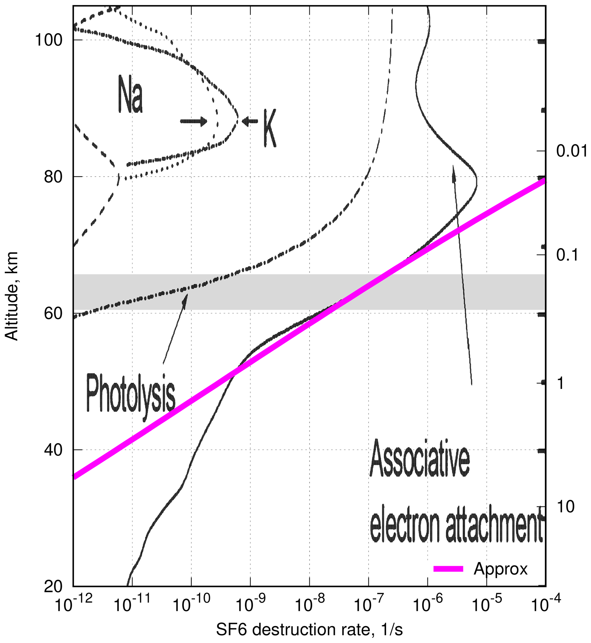
Figure 2The vertical profiles of SF6 destruction rate (after Totterdill et al., 2015) and its approximation in the range of 55–75 km, given by Eq. (6).
As an approximation to the vertical profile of the destruction rate in an altitude range of 50–80 km, we have fitted the corresponding part of the curve in Fig. 9a of Totterdill et al. (2015) with a power function of pressure (magenta line in Fig. 2):
where τ is the lifetime of SF6 at the altitude corresponding to pressure p.
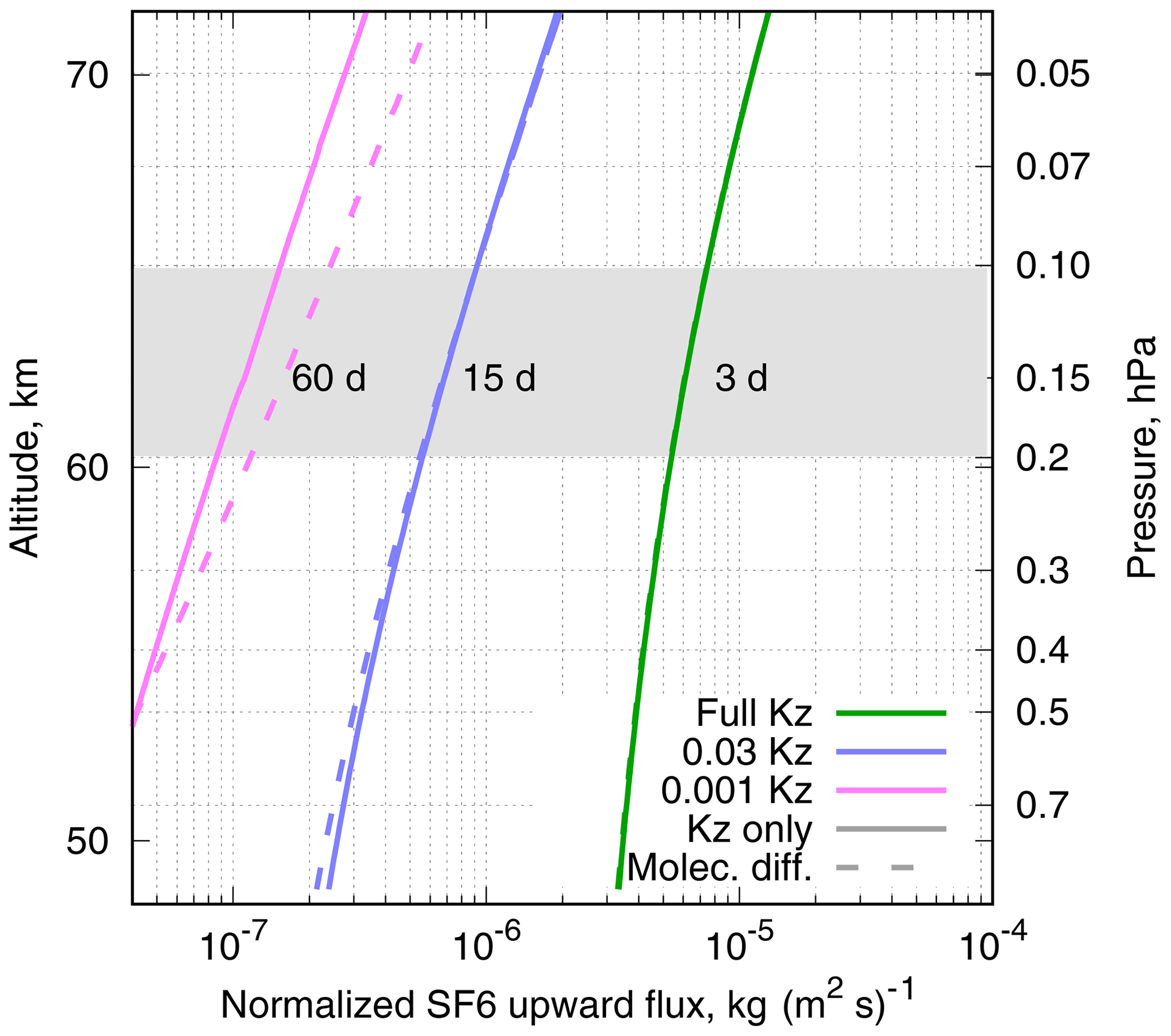
Figure 3Vertical profiles of steady-state upward flux of SF6 normalized with mass mixing ratio, F(p)∕ξ(p), for eddy-diffusivity and lifetime profiles given by Eqs. (1) and (6). The topmost model layer of SILAM and effective lifetimes of SF6 there due to the destruction in the mesosphere for different Kz profiles are given.
The topmost level of the ERA-Interim meteorological dataset is located at 0.1 hPa, which is below the layer where the destruction of SF6 occurs. Therefore, we have to put a boundary condition on our simulations to account for the upward flux of SF6 through the upper boundary of the simulation domain. For that, we assume that the SF6 distribution above the computational domain top is in equilibrium with the destruction and the vertical flux.
Assuming the profiles for Kz(p) and the SF6 lifetime τ(p) are given by Eqs. (1) and (6), one can obtain a steady-state distribution of the mass-mixing ratio, ξ, of SF6 due to destruction in the mesosphere at any point where both Eqs. (1) and (6) are valid and vertical advection is negligible. The latter assumption implies that the diffusive vertical flux overwhelms the advective one. The validity and implications of neglecting the regular vertical transport are discussed below. The steady-state profile of ξ can be obtained from a solution of the steady-state diffusion equation with a sink:
where ρ(p) is air density, g is acceleration due to gravity, and the upward flux of SF6 is given by
The above equation was solved numerically as a boundary value problem with unit mixing ratio at a height of 1 hPa and vanishing flux, F(p) at p=0, for the set of Kz profiles. The shooting method with bisection was used to get the steady-state profiles of ξ(p) and F(p), corresponding to ξ(1 hPa)=1. For all considered cases, the flux F(p) decreased by several orders of magnitude already at the level of a few pascals (Pa), i.e. below the maximum of the depletion profile of Totterdill et al. (2015), indicating that the particular shape of τ(p) above that level does not influence the fluxes at the domain top (0.1 hPa). The steady-state upward flux of SF6 F(p) normalized with the corresponding mixing ratio at each pressure, F(p)∕ξ(p), for the three test profiles of Kz is shown in Fig. 3 with solid lines.
The gravitational separation can be accounted for by introducing a term responsible for molecular diffusion and its equilibrium state Eq. (4) into the vertical flux Eq. (8) :
The profiles of F(p)∕ξ(p) resulting from F(p) in Eq. (7) are given in Fig. 3 with dashed lines. The magnitude of F(p)∕ξ(p) gives an equivalent regular vertical air-mass flux that would result in the same vertical flux of SF6 if it were passive and non-diffusive. The equivalent regular vertical velocity ωeq (in units of the Lagrangian tendency of a parcel pressure due to vertical advection) can be expressed as
Accounting for molecular diffusion may either enhance or reduce the upward flux of SF6 in the model. Along with setting the equilibrium state with the bulk of a heavy admixture being in the lower layers, molecular diffusion provides additional means for transport to the upper layers where the destruction occurs. For very low eddy diffusivities, the molecular diffusion is a sole mechanism of the upward transport of SF6 towards depletion layers. For higher eddy diffusivity, the effect of molecular diffusion and gravitational separation becomes negligible.
For the model consisting of stacked well-mixed finite layers, the loss of SF6 from the topmost layer due to the steady upward flux would be proportional to the SF6 mixing ratio in the layer. This loss of mass is equivalent to a linear decay of SF6 in the layer at a rate
where Δp is pressure drop in the layer.
In the upper layer of our simulations (between 0.1 and 0.2 hPa, grey rectangle in Fig. 3), the SF6 lifetime τ due to turbulent diffusion is about 3 d for Kz of Eq. (1). After scaling the Kz(p) profile with factors of 0.03 and 0.001, one gets the lifetimes of 15 and 60 d, respectively. Note that the molecular diffusion sets the upper limit to the SF6 lifetime in the topmost model layer: it can not be longer than 60 d for the 0.1–0.2 hPa layer. Close to this regime, the system becomes insensitive to the actual profile and values of the turbulent diffusion coefficient. The loss of SF6 through the domain top was implemented as a linear decay of SF6 in the topmost model layer, at a rate corresponding to the Kz(p) profile used in each simulation.
3.4 Simulated tracers
SILAM performs the 3D transport by means of a dimension split: transport along each dimension is performed separately as 1D transport. To minimize the inconsistency between the tracer transport and air-mass fluxes caused by the dimension split at finite time step, the splitting sequence has been inverted at each time step. The residual inconsistency was resolved by using a separate unity tracer, which was initialized to the constant mass mixing ratio of 1 at the beginning of a simulation. Should advection be perfect, the concentration of the unity tracer would be equivalent to air density (mixing ratio would stay equal to 1). The mixing ratios of the simulated tracers were then evaluated as a ratio of the tracer mass in a cell to the mass of the unity tracer.
In order to assess the effects of gravitational separation and destruction on the atmospheric distribution of SF6, we used four tracers: SF6 as a passive tracer sf6pass, SF6 with gravitational separation but no destruction sf6nochem (no chemistry), SF6 with destruction but no gravitational separation sf6nograv, and SF6 with both gravitational separation and destruction in the upper model level sf6.
All SF6 tracers had the same emission according to the SF6 emission inventory (Rigby et al., 2010). The inventory covers 1970–2008 and was extrapolated with a linearly growing trend of 0.294 Gg yr−2 until July 2016. The last 2.5 years were run without the SF6 emissions to evaluate its destruction rate. Note that the emission extrapolation gives 9.4 Gg yr−1 for 2016, which is somewhat higher than the later estimate of 8.8 Gg yr−1 (Engel et al., 2018).
Besides the four SF6 tracers, we used a passive tracer emitted uniformly at the surface at constant rate during the whole simulation time and an ideal-age tracer. The ideal-age tracer is defined as a tracer whose mixing ratio ξia obeys the continuity equation (Waugh and Hall, 2002)
(where ℒ is the advection–diffusion operator), and boundary condition ξia=0 at the surface. The ideal-age tracer is transported as a regular gaseous tracer and updated at every model time step Δt with the unity tracer correction:
where Mia and Munity are masses of the ideal-age tracer and of the unity tracer in the grid cell. The mixing ratio of the ideal-age tracer is a direct measure of the mean age of air in a cell, so the tracer is a direct Eulerian analogue of the time-tagged Lagrangian particles with clock reset at the surface. Note that the AoA derived from the ideal-age tracer and AoA from a passive tracer with a linearly growing near-surface mixing ratio are equivalent (Waugh and Hall, 2002), and implementation of both provides a redundancy needed to ensure self-consistency of our results.
The simulations were performed with four eddy-diffusivity profiles described in Sect. 3.1 and the corresponding destruction rates of sf6 and sf6nograv tracers in the uppermost model layer. All runs were initialized with the mixing ratios from the final state of a special initialization run. The initialization simulation with 0.1-Kz eddy diffusivity was started from 1970 with zero fields for all tracers, except for the unity tracer that was set to unity mixing ratio. The simulation used 1970–1989 emissions for SF6 species from the same inventory as for the main runs (Rigby et al., 2010), and it was driven with the twice repeated ERA-Interim meteorological fields for 1980–1989. The mixing ratios of all SF6 tracers at the end of the initialization run were scaled to match the total SF6 burden of 20.17 Gg in 1980 (Levin et al., 2010).
4.1 Gravitational separation and mesospheric depletion
To evaluate the relative importance of gravitational separation, mesospheric depletion, and their effect on the SF6 concentrations, we compared the simulations for the SF6 tracers and evaluated the relative reduction of the SF6 content in the stratosphere due to these processes. As a conservative estimate of the reduction, we evaluated the relative differences between the tracers in the latitude belt of 70–85∘ S, since both processes have the most pronounced effect in the southern polar vortex, where the downwelling of Brewer–Dobson circulation is the strongest.
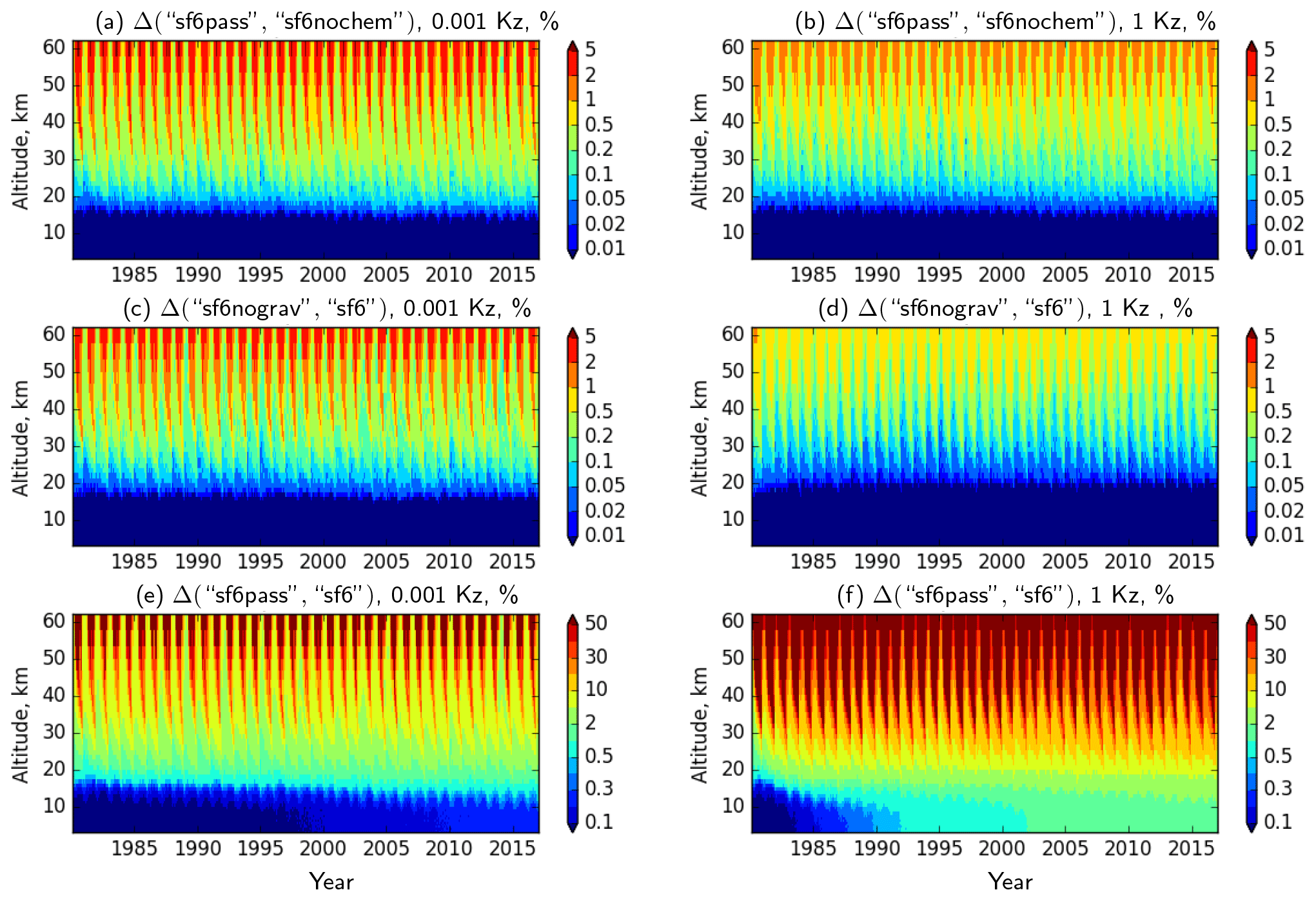
Figure 4The relative reduction of the SF6 content (in %) at 70–85∘ S due to gravitational separation with (a, b) and without (c, d) depletion and due to the combined effect of depletion and separation (e, f) at two extreme Kz cases. Note the different colour scales for (e) and (f).
Hereafter we quantify the relative difference between atmospheric contents of two SF6 tracers, “X” and “Y” as
The relative differences for the SF6 tracers in the southern polar region (70–85∘ S) simulated with two extreme Kz profiles is given in Fig. 4 as a function of time and altitude. Note that every 5 % of the decrease of SF6 with respect to its passive counterpart corresponds to about 1 year of a positive bias in AoA derived from the SF6 mixing ratios.
The reduction of the SF6 content due to gravitational separation, if the mesospheric depletion is disabled, is given by the relative difference of sf6nochem and sf6pass (Fig. 4a, b). Expectedly, the effect of gravitational separation is most pronounced for the case of low eddy diffusivity (0.001-Kz), and the reduction of SF6 in the altitude range of 30–50 km reaches 2 %–5 %. In the case of strong mixing, the effect of separation is about 1 %.
The reduction of the SF6 content due to gravitational separation in the presence of stratospheric depletion is given by the relative difference of sf6nograv and sf6 tracers. The effect of the separation for low Kz is very similar between the depletion and no-depletion cases (Fig. 4c vs. Fig. 4a). Depletion reduces the effect of the gravitational separation for high Kz (Fig. 4b vs. Fig. 4d). Regardless of depletion, stronger Kz reduces the effect of the gravitational separation; however, the latter is still non-negligible if precisions of the order of a month for AoA are required.
The combined effect of depletion and gravitational separation is seen in the relative difference of sf6pass and sf6 tracers (Fig. 4e and f). For both Kz cases, the effect of depletion is stronger than the diffusive separation by more than 1 order of magnitude. Regardless of the Kz profiles, the reduction exceeds 50 %, which roughly corresponds to 10 years of an offset in the apparent AoA.
In all cases the reduction of the SF6 content has a strong annual cycle associated with the cycle of the downwelling in winter and the upwelling in summer. Besides, the reduction has a noticeable inter-annual variability that poses substantial difficulties for applying a consistent correction to the apparent AoA. Contrary to the former two comparisons, strong eddy mixing leads to a strong reduction of SF6 since it intensifies the transport to the depletion layers and thus enhances the depletion rate.
The simulations for different Kz have been initialized with the same state obtained from a separate spin-up simulation with 0.01-Kz, which was scaled to match total burden of SF6 in 1980. Thus a relaxation of the SF6 vertical distribution during the first few years of the simulations is clearly seen in Fig. 4. For the 1-Kz case (Fig. 4f), the gradual increase of the difference between SF6 and its passive version in the troposphere can be seen as well. The rate of this increase is about 0.5 % per 39 years of the simulations. This rate should not be confused with the depletion rate of SF6 in the atmosphere since the difference is a combined effect of depletion and growth of emission rate, despite the fact that the latter is exactly the same for both tracers.
The above comparison indicates that depletion has the stronger effect on the SF6 mixing ratio in the upper stratosphere than gravitational separation and molecular diffusion. However, the important role of molecular diffusion in the model is that it maintains the upward flux towards the mesosphere in the simulations even if the eddy diffusivity ceases.
Further in this paper only the sf6pass and sf6 tracers will be used.
4.2 Evaluation against balloon profiles
The tropospheric concentrations of SF6 in our simulations have been insensitive to the SF6 destruction or to the eddy-diffusivity profiles in the stratosphere. The difference in the modelled profiles can, however, be seen above the tropopause. For comparison, we took the simulations with prescribed eddy diffusivity in the stratosphere (1-Kz, 0.03-Kz, and 0.001-Kz; see Sect. 3.1) and with dynamic eddy diffusivity ECMWF-Kz. The simulations were matched with the stratospheric balloon observations (Fig. 5) published by Patra et al. (1997), Engel et al. (2006), Ray et al. (2014), and Ray et al. (2017).

Figure 5Observed SF6 balloon profiles and corresponding daily-mean SILAM profiles for the date of observations. The observational data obtained from Patra et al. (1997), Ray et al. (2014, 2017), and Engel et al. (2006) are for (a)–(d) correspondingly. The observation uncertainties are about 2 % (1σ) for Hyderabad profiles (a) and smaller than the size of the symbol for Kiruna profiles (b, d). The model profiles from the WACCM model are from Ray et al. (2017).
Two balloon profiles observed at Hyderabad (17.5∘ N, 78.6∘ E) in 1987 and 1994 by Patra et al. (1997) indicate an increase of the SF6 content during the time between the soundings (Fig. 5a). Both profiles have a clear transition layer from tropopause at ∼17 km to the undisturbed upper stratosphere above ∼25 km. The simulated profiles agree quite well with the observed profiles, except for the most diffusive case that gave notably smoother profiles and somewhat overstated SF6 mixing ratios due to too strong upward transport by diffusion through the tropopause and in the lower stratosphere.
The profile in Fig. 5b has been obtained from Kiruna (68∘ N, 21∘ E) in early spring 2000 during the SAGE III Ozone Loss and Validation Experiment, SOLVE, (Ray et al., 2002) with the lightweight airborne chromatograph (Moore et al., 2003). The profile is affected by the polar vortex and clearly indicates a strong reduction of SF6 with height with a pronounced local minimum at 32 km. The corresponding SILAM profiles tend to overestimate the SF6 volume mixing ratio (vmr). The SF6 profiles for ECMWF-Kz and 0.001-Kz match each other, since vertical mixing is negligible in both cases. The most diffusive profile, 1-Kz, has the strongest depletion in the upper part but the largest deviation from the observations below 20 km. The intermediate-diffusion profile (0.03-Kz) is almost as close to the observations as the non-diffusive profile. Moreover, the 0.03-Kz profile has a minimum at the same altitude as the observed one, albeit the modelled minimum is substantially less deep.
For comparison, Fig. 5b also contains monthly-mean profiles from the WACCM simulations by Ray et al. (2017). The WACCM profiles match very well with the observations below 17 km but turn nearly constant above, thus under-representing the depletion of SF6 inside the polar vortex. Monthly-mean SILAM profiles (not shown) were much closer to the plotted daily profiles than to the ones of WACCM. However, the WACCM simulations did not include the electron attachment mechanism.
For the mid-latitude profile in Fig. 5c from Aire-sur-l'Adour, France (43.7∘ N, 0.3∘ W), all SILAM profiles except for 1-Kz fall within the observational error bars provided together with the data by Ray et al. (2017). Similar to the Kiruna case in Fig. 5b, the SILAM profiles are smoother than the observed ones and are unable to reproduce the sharp transition at 20 km.
Another profile from within the polar vortex (Fig. 5d) was observed at the same Kiruna site as the one in Fig. 5b, but three years later. The observed profile also has a minimum that is much deeper than in the modelled profiles. Similar to the case in Fig. 5b, the 0.03-Kz profile is the only one that has a pronounced minimum at the same altitude as the observed one. The minimum is a result of the spring breakdown of the polar vortex when a regular downdraught ceases and atmospheric layers decouple from each other. The reduced depth of the modelled minimum is probably caused by insufficient decoupling of the layers in the driving meteorology.
In all above cases, the 1-Kz profile is clearly far too diffusive in the non-polar cases, whereas for the Kiruna cases it overstates the lower part of the profiles and smears out the vertical structure of the profiles further above the tropopause. The SF6 profiles simulated with ECMWF-Kz and 0.001-Kz match each other in all simulations, since vertical mixing is negligible in both cases. The SF6 resulting from the 0.03-Kz case appears to be the most realistic out of the four considered simulations: they are close to the observed ones and have the local minima at the correct altitudes for both Kiruna profiles.
4.3 Evaluation of SF6 against MIPAS data
The MIPAS observations provide the richest observational dataset for the stratospheric SF6 profiles. However, each individual observation has a substantial retrieval noise error, which is noticeably larger than the difference between the observation and any of the SILAM simulations. The largest diversity of the modelled SF6 profiles was observed in polar regions; therefore, below we show the mean profiles for each season in the southern and the northern polar areas. Besides that, we consider statistics of the model performance against MIPAS measurements in the lower and upper stratosphere separately. For simplicity, we do not show the statistics for the ECMWF-Kz runs, since they are very similar to the ones for 0.001-Kz.
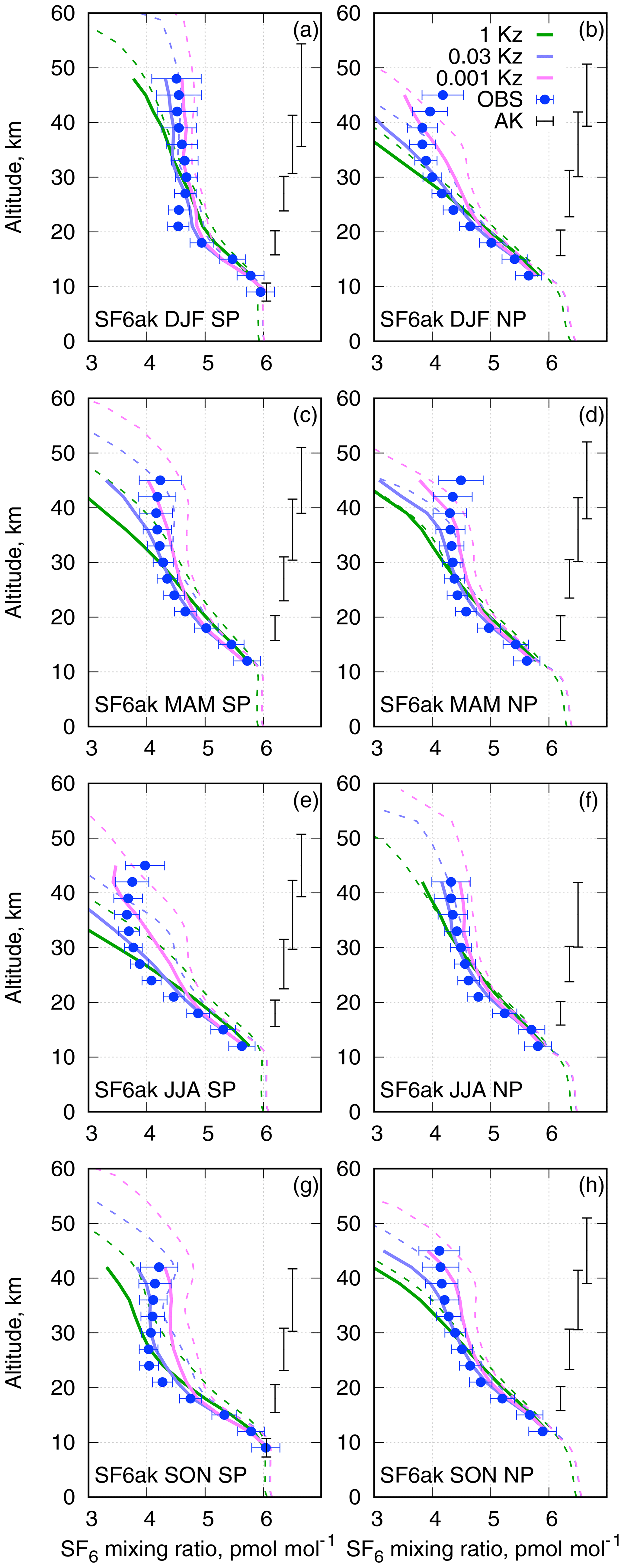
Figure 6Seasonal mean co-located SILAM SF6 and MIPAS profiles for 2007, for southern and northern polar regions. Typical ranges covering 75 % of the averaging kernel are given with the error bars at the right-hand side of each panel. The horizontal error bars indicate systematic uncertainties of the observations that are fully correlated among profiles and do not cancel out when averaging over a large number of measurements. Dashed lines are zonal-mean SILAM profiles for a given season taken without co-location.
For the comparison, the daily-mean model profiles were co-located to the observed ones in space and time, after which an averaging kernel of the corresponding MIPAS profile was applied to the SILAM profile. For the comparison, we took only the data points with all of the following criteria met:
-
MIPAS visibility flag equals 1;
-
MIPAS averaging kernel diagonal elements exceed 0.03;
-
MIPAS retrieval vertical resolution, i.e. the full width at the half maximum of the row of the averaging kernel, is better than 20 km;
-
MIPAS volume mixing ratio noise error of SF6 is less than 3 pmol mol−1.
The mean seasonal profiles of the SF6 mixing ratio for southern and northern polar regions derived from the MIPAS observations and the SILAM simulations for 2007 are given in Fig. 6. In order to facilitate the comparison of our evaluation with the earlier study of Kovács et al. (2017), we have chosen the same year and same layout of the panels as Fig. 3 there. The main differences between Kovács et al. (2017) and the current evaluation are the following.
-
We used averages of co-located model profiles (bold lines). The non-co-located seasonal- and area-mean model profiles are given as thin dashed lines for comparison.
-
We use a newer version of the MIPAS SF6 data with considerably larger values (up to 0.6 pmol mol−1) in the upper stratosphere, compared to the version that was used by Kovács et al. (2017).
-
The horizontal error bars for the observed data indicate that the systematic error component is fully correlated among the profiles and does not cancel out by averaging or, in other words, the estimate of a possible bias, as analysed by Stiller et al. (2008). These errors are of the order of 4 % (below 30 km) up to 10 % (at 60 km). The contribution of the retrieval noise error is essentially negligible due to averaging. The error bars shown by Kovács et al. (2017) are noticeably larger, probably indicating that they are for the individual observed values rather than the uncertainties of the mean.
-
We use 3 km vertical bins for the profiles to make the points in the MIPAS profiles distinguishable.
-
We also plot the vertical extent of the averaging kernels corresponding to their half widths.
First of all, there is a substantial difference between the co-located and non-co-located model profiles. The difference is caused by the uneven sampling of the atmosphere by the satellite both in space and in time. In particular, MIPAS, being a polar-orbiting instrument, makes more profiles per unit area closer to the pole than further away. The difference gets somewhat reduced if one uses equal weights for all model grid cells instead of area-weighted averaging, especially for wide latitude belts. The major difference comes probably from the inability of MIPAS to retrieve SF6 profiles in the presence of polar stratospheric clouds that clutter lower layers of the stratosphere and make the sampling of polar regions quite uneven both in time and in the vertical. This hypothesis agrees with the fact that the difference is most pronounced for the winter pole, especially for the South Pole in JJA, and almost invisible at a summer pole.
The comparison in Fig. 6 shows that the profiles from the SILAM simulations agree quite well to the observations in the altitude range below 20–25 km, with the most diffusive, 1-Kz, slightly overestimating the SF6 mixing ratios. In the range above 25 km, the 1-Kz profiles indicate a decrease of SF6 with altitude that is too fast. The 0.03-Kz profiles give the best results up to ∼40 km, except for the South Pole in JJA and the North Pole in DJF.
An interesting feature of the winter-pole MIPAS profiles is an increase of the SF6 mixing ratio above 40 km. This increase might be caused by issues with retrievals as the systematic errors of the retrievals increase with altitude. However, non-monotonic profiles can occur due to the mean atmospheric dynamics (see the non-co-located 0.001-Kz profile in Fig. 6g).
None of the model setups are capable of reproducing the observations above 40 km. Wintertime poles also pose a problem to the model. The disagreement indicates a deficiency in the model representation of air flows in the upper part of the domain caused by insufficient vertical resolution of ERA-Interim in the upper stratosphere and lower mesosphere and a lack of pole-to-pole circulation. This discrepancy is in line with the comparisons in Fig. 5 for polar regions. The model tends to overstate the SF6 content in the lower part of the polar vortex and understate it above 40 km.

Figure 7Time series of monthly scores for the SILAM SF6 mixing ratios for the whole period of the MIPAS observations in the altitude range of 10–35 km. The statistics are standard deviations of model–measurement difference (SD), absolute bias, and normalized mean bias (NMB). The statistics of the model mixing ratios extracted at nominal MIPAS altitudes are given as thin lines.
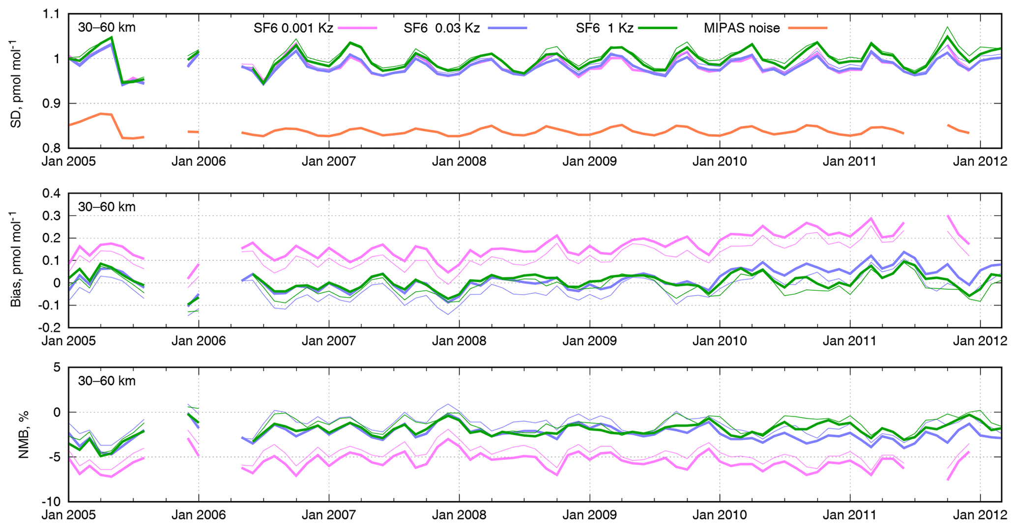
We also computed statistical scores of the simulated SF6 mixing ratios for each month of the MIPAS mission. The statistics were computed separately for the altitude ranges of 10–35 km (Fig. 7) and 30–60 km (Fig. 8). As the difference in the statistical scores between the three selected simulations is quite minor, we used only observations with the retrieval target noise error below 1 pmol mol−1.
The root-mean-square error turned out to be mostly controlled by the bias, and it does not allow for a clear distinction between the simulated cases. In order to disentangle the effect of bias, we have calculated the standard deviation of the model–measurement difference (SD), absolute bias, and normalized mean bias (NMB):
where M and O are modelled and observed values, respectively, and 〈⋅〉 denotes averaging over the selected model–observation pairs for the given range of times and altitudes. Along with the SD, we have plotted the RMSE of the observations due to the retrieval noise in the original MIPAS data, labelled as “MIPAS noise” in the top panels of Figs. 7 and 8.
In the altitude range of 10–35 km, the SD of model–measurement difference is uniform in time with minor peaks in August–September (Fig. 7). The level of the noise error constitutes about 85 % of the total model–measurement difference. Application of the averaging kernel to the model profiles reduces the SD. The intermediate-diffusivity case, 0.03-Kz, clearly shows the least SD uniformly over the whole observation period; the same case indicates the least absolute bias.
In the range of 30–60 km altitudes (Fig. 8), the level of the retrieval noise is noticeably higher than in the lower stratosphere. The least biased case is 1-Kz, which, however, has the largest SD. The SDs of 0.03-Kz and 0.001-Kz are on par, but the latter has the strongest bias. Thus for this altitude range the intermediate-diffusivity case also shows the best performance.
Note the slight increase of the model bias after 2009, which is likely caused by our overestimating of the emission rates since that time (see Sect. 3.4). This increase of the bias does not appear in Fig. 8 due to the delay in the response of the content in the upper layers to the changes in surface emissions.
4.4 Lifetime of SF6 in the atmosphere
In order to estimate the atmospheric lifetime of SF6, we turned off the emission of all SF6 tracers in July 2016 and let the model run until the end of 2018 without emissions (Fig. 9). The decrease of the simulated burden after the emission stop can be used to estimate the removal rate from the atmosphere.
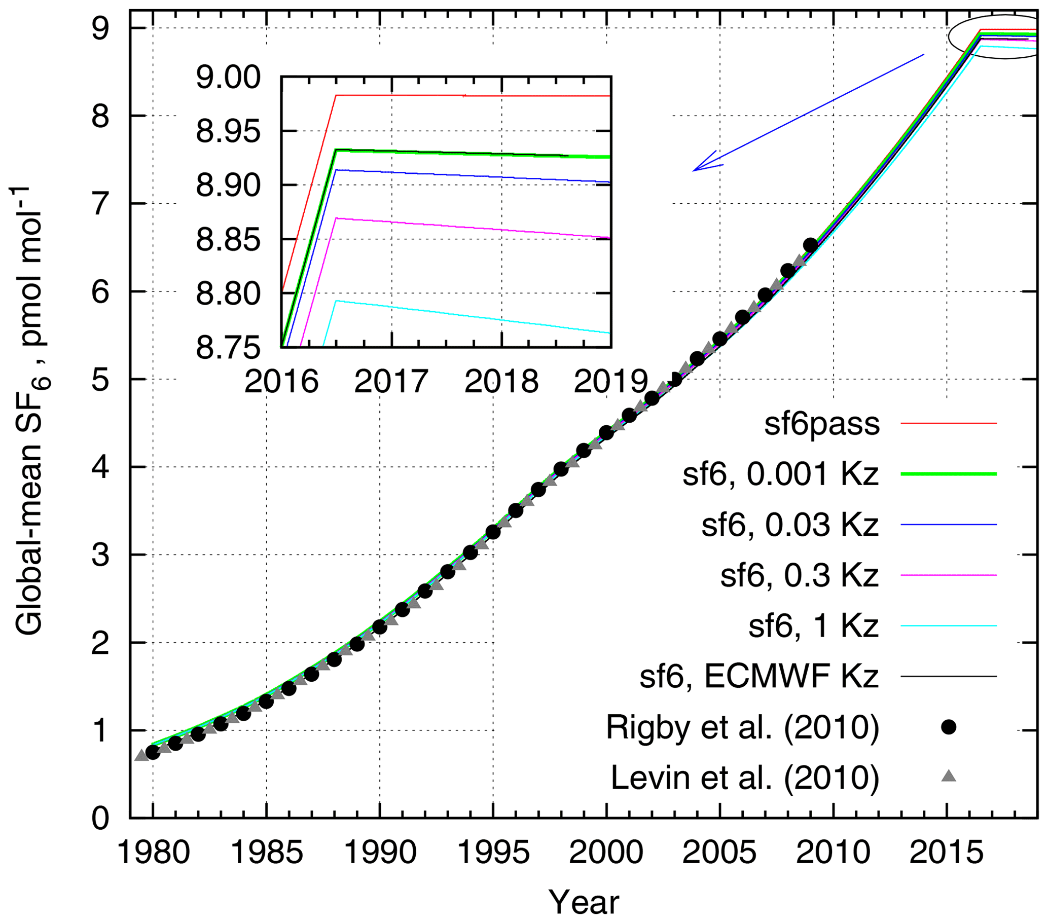
Figure 9The time series of mean mixing ratio of SF6 in the atmosphere simulated with emissions stopped in July 2016. The total burdens by Levin et al. (2010) and by Rigby et al. (2010) are shown for comparison.
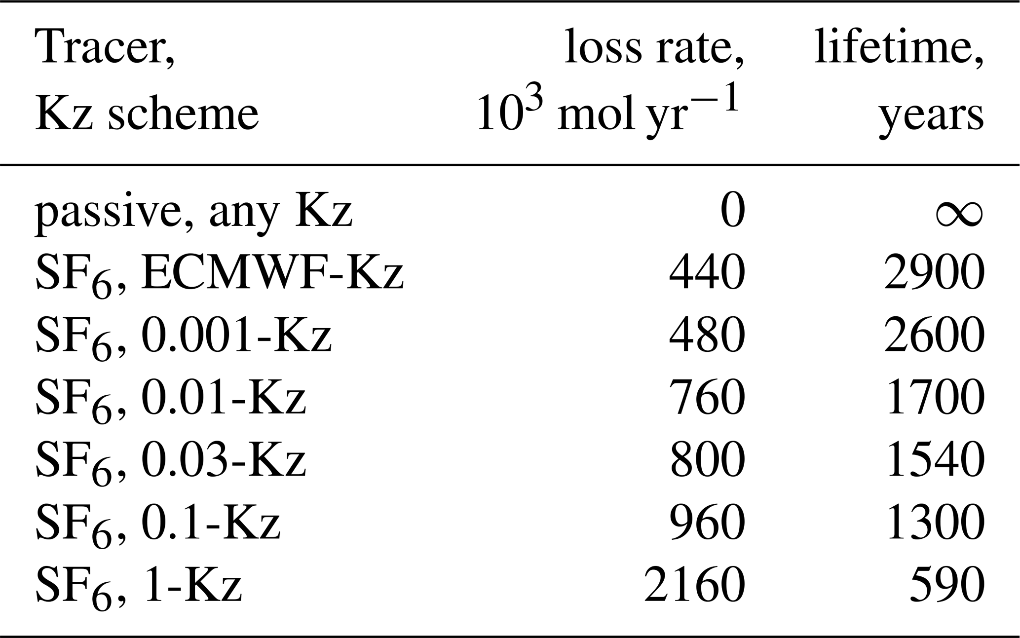
Table 1SF6 destruction rate after stopping the emissions and corresponding lifetimes. Mid-2011 burden of 1.27×10⁹ moles is used as a reference for the lifetime estimate.
Time series of the total burden of SF6 in the atmosphere in the simulations are given in Fig. 9. For easier comparison to the observed mixing ratios, the burden has been normalized with 1.78×10²⁰ moles – the total amount of air in the atmosphere – to get the mean mixing ratio. The tabulated values for the atmospheric burden of SF6 from Levin et al. (2010) and Rigby et al. (2010) are given for comparison. Since the removal of SF6 from the atmosphere is mostly controlled by the transport towards the depletion layer, the vertical exchange is the key controlling factor.
The decrease of the atmospheric SF6 content after the emission stop is given in the inset in Fig. 9. As expected, after July 2016 the content of passive SF6 stays constant, while the others begin to decrease at a rate that depends on the transport properties in the stratosphere with the faster removal for the stronger eddy diffusivity. The removal rate is driven by the SF6 content in the upper stratosphere, which is not in equilibrium with the total atmospheric content. A typical delay between the SF6 mixing ratio in the troposphere and the upper stratosphere, i.e. the AoA in the topmost model layer, is about 5–6 years. Therefore, for a reference we used the total amount of atmospheric SF6 5 years before the emission stop, i.e. 1.23×10⁹ mol, which corresponds to the mean mixing ratio of 7 pmol mol−1. Dividing the destruction rate with the reference amount, one gets the range of corresponding simulated SF6 lifetimes in the atmosphere: 600 to 2900 years. Despite the range of the tested diffusivities of 3 orders of magnitude, the loss rate varies only within a factor of 5 (Table 1).
The term “lifetime” implies a linear decay; however, due to emissions the distribution of SF6 in the atmosphere is far from equilibrium, so the decay is not proportional to the burden. A more accurate way to estimate the lifetime would be to perform a multi-decade simulation without sources to get the distribution into a quasi-equilibrium with the mesospheric sink. In such a quasi-equilibrium the model of linear decay of SF6 in the whole atmosphere becomes applicable and the lifetime can be estimated as a simple ratio of the burden to the loss rate. The uncertainty in the equilibrium burden corresponding to the modelled loss rates in Table 1 can be estimated as the range of AoA in the upper stratosphere (∼0.5 years) divided by the growth rate of the burden (0.04 yr−1), i.e. about 2 %. A larger uncertainty comes from the over-simplistic parametrization of the loss in the model, which is more difficult to quantify.
The best-performing simulation, 0.03-Kz, resulted in 1540 years lifetime. Given the uncertainties above, it meets the ranges suggested by earlier studies. It is in a good agreement with the range of 800–3200 years from the model studies (Ravishankara et al., 1993; Morris et al., 1995), and it is close to the upper bound of the 580–1400 years range recently obtained by Ray et al. (2017) from the balloon profile given in Fig. 5b.
Our estimate is also slightly above the range given by Kovács et al. (2017), who obtained 1120–1475 years. However, in the simulations by Kovács et al. (2017) the mixing ratios of SF6 in the stratosphere and the lower mesosphere were noticeably higher than those retrieved by MIPAS and practically flat in the range of 30–50 km. Such modelled profiles likely indicate a vertical exchange in the model that is too strong; a loss that is too strong, as a consequence; and corresponding low bias of the estimated lifetime.
5.1 Eddy diffusivity and simulated AoA
The effect of the vertical eddy diffusivity on AoA in the stratosphere was evaluated with the same set of three prescribed and one dynamic Kz profiles, as for SF6 simulations. An example of annual-mean distributions of AoA is given in Fig. 10. The Hunten (1975) Kz profile (Fig. 10a) gives AoA in the stratosphere of about 3.5 years. It is much shorter than the estimates of the stratospheric AoA (e.g. Waugh, 2009; Engel et al., 2009) from the observations of various tracers. Three other profiles of Kz result in almost identical average distributions of AoA with typical stratospheric AoA of 5.5 years, which agrees quite well with the experimental estimates. In these cases AoA is controlled by the transport with mean winds. Since 0.03-Kz profiles result in the most realistic distribution of SF6 in our simulations, in the current section we will use simulated distributions of tracers with this parameterization.
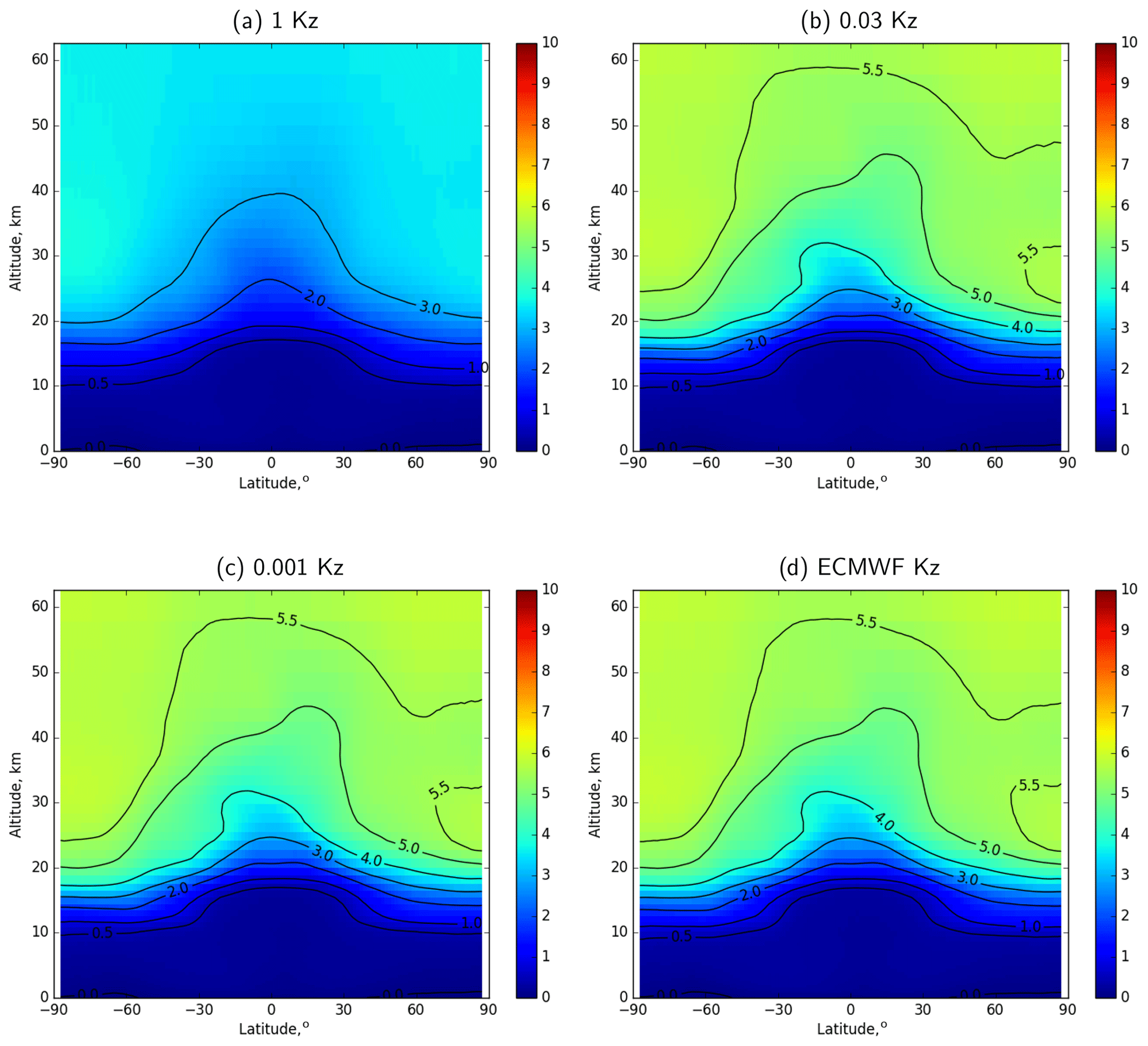
Figure 10The zonal-mean spatial distribution of the ideal-age AoA for 2011 calculated for different eddy-diffusivity profiles.
5.2 AoA and apparent SF6 AoA
The AoA for all tracers (except for the ideal age) was calculated as a simple time lag between the mixing ratio at each point of the domain and the mean near-surface mixing ratio. As it has been pointed out by Waugh and Hall (2002), this lag equals to AoA only in the case of a fully passive tracer with linearly growing (or decreasing) near-surface mixing ratio. Corrections have been applied to the AoA derived from SF6 in many studies (Volk et al., 1997; Stiller et al., 2008, 2012; Engel et al., 2009) to account for non-linear growth of the near-surface SF6 mixing ratio and for its mesospheric sink. The corrections rely heavily on various assumptions that can hardly be rigorously verified. Therefore, in this study we do not apply any corrections to the AoA derived from the time lags of tracers. The corrections and assumptions behind them are discussed in Sect. 6.
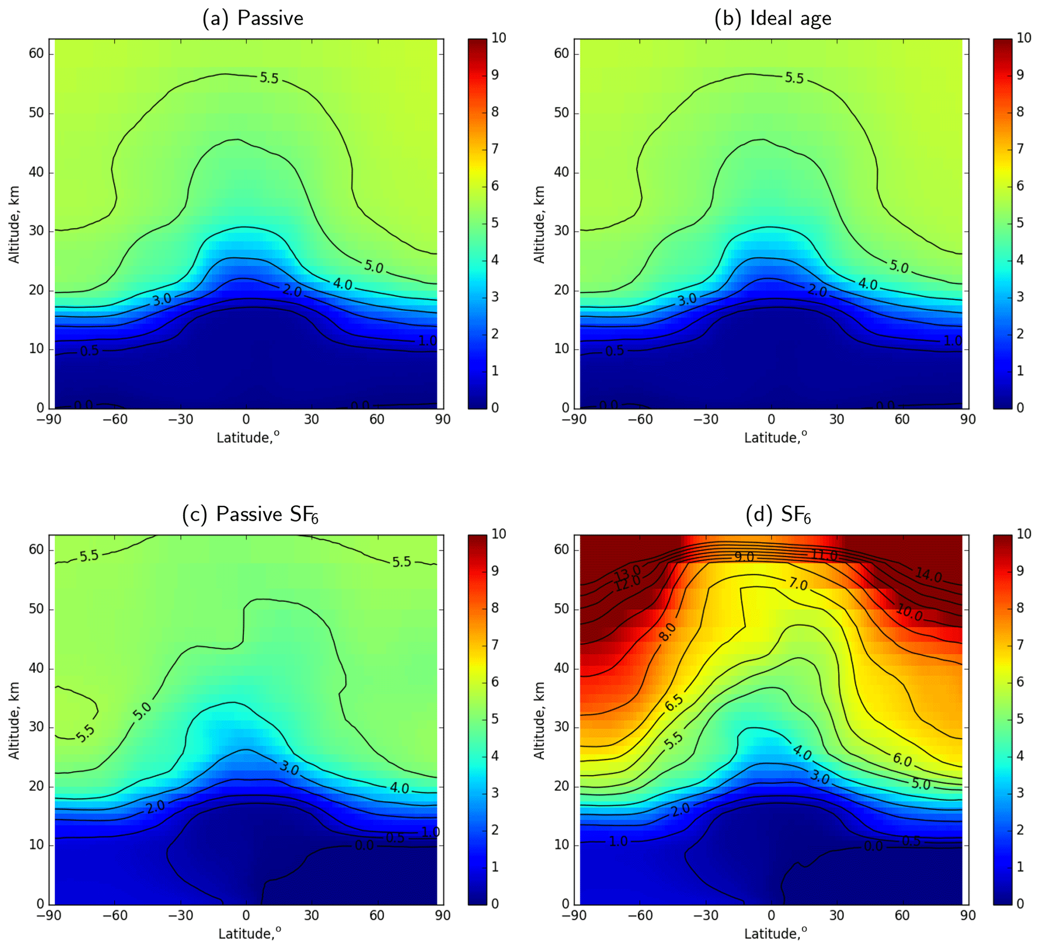
Figure 11Zonal-mean distributions of atmospheric AoA simulated with passive, ideal-age, and two SF6 tracers (average for 2012).
The constant-rate emission of the passive tracer resulted in almost linear growth of its near-surface mixing ratio after the spin-up. The latter makes the age derived from the passive tracer equivalent to the age derived from the ideal-age tracer. The resulting distributions are indeed very close to each other (Fig. 11a and b). The agreement confirms the self-consistency of the transport procedure since the tracers have opposite sensitivity to the advection errors: higher mixing ratios correspond to younger air for the accumulating tracers, while for the ideal-age tracer higher mixing ratios correspond to older air. The remaining differences are caused by spatial inhomogeneities of near-surface mixing ratio of the passive tracer due to variations in the near-surface air density.
The distribution of the AoA derived from sf6pass (Fig. 11c) is qualitatively similar to the ideal-age one; however, one can see substantial differences. The negative AoA in the northern troposphere for the sf6pass tracer is caused by the predominant location of the sources in the Northern Hemisphere, so the concentrations there exceed the global-mean levels. The growing rate of the SF6 emissions leads to the faster-than-linear increase of near-surface mixing ratios, which leads to an old bias of up to 3–5 months of the sf6pass AoA. This old bias has been one of the drawbacks of the SF6 AoA pointed out by Garcia et al. (2011).
The ages shown in Fig. 11a–c agree well with the ages derived from the in situ observations of SF6 and CO2 at the 25 km altitude by Waugh and Hall (2002). They also agree quite well with the earlier simulations with five climate models that give annual mean ages in the upper stratosphere between 4.5 and 5.5 years (Butchart et al., 2010). The simulations result in about 1–1.5 years younger air than diabatic mean age obtained with the Lagrangian model computations of Diallo et al. (2012) (Fig. 11 is directly comparable with Fig. 2 there) and about 1 year older air than kinematic mean age. Since our preprocessor of wind fields differed strongly from that by Diallo et al. (2012), this similarity is an important indicator of consistency of the numerical procedures applied in both studies.
A substantial disagreement, however, exists with the ages derived from the MIPAS satellite observations (Stiller et al., 2012; Haenel et al., 2015). The authors calculated ages exceeding 10 years in the polar areas and in the upper stratosphere. The reason for the disagreement follows from the above analysis: SF6 can neither be considered a passive tracer nor does its mixing ratio in the troposphere grow linearly with time. Denoting the AoA derived from the SF6 profiles as “apparent AoA” (Waugh and Hall, 2002), we calculated it from the SILAM-predicted SF6 profiles, which, as shown above, agree well with AoA derived from MIPAS. The resulting model-based apparent AoA (Fig. 11d) is indeed much older than the ideal-age AoA. The distribution of the apparent SF6 AoA agrees with the AoA retrieved from MIPAS SF6 profiles by Haenel et al. (2015): well over 5 years AoA around the Equator with well over 10 years AoA in the polar regions.
The effect of the apparent over-ageing in the stratosphere due to the subsidence of the mesospheric air was estimated by Stiller et al. (2012) to be a fraction of a year in the upper stratosphere. Earlier experimental balloon studies (Strunk et al., 2000) indicated an up to 3.5-year difference between CO2 and SF6 ages. In our simulations, the over-ageing due to the SF6 depletion and other factors discussed in the previous sections is much stronger and affects the whole stratosphere.
5.3 Trends in apparent AoA
Changes in the AoA have been used in many studies as an indicator of changes in the atmospheric circulation. In order to evaluate the effect of the way the AoA is computed on its trend, we have calculated trends of the apparent AoA at different altitudes and latitudes for 11 years (2002–2012). This period roughly covers the MIPAS mission and allows for comparison with trends reported by Haenel et al. (2015).
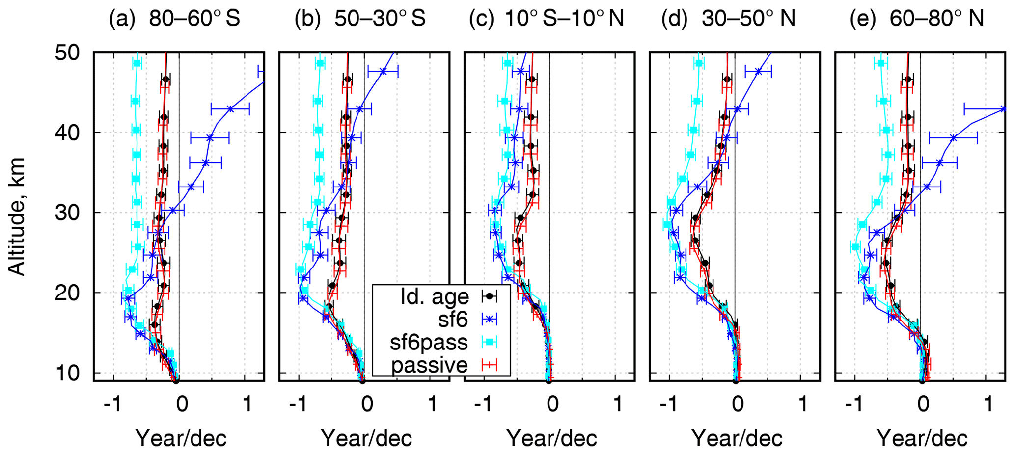
Figure 12Vertical profiles of the simulated age of air linear trends over 11 years (2002–2012) for example latitude belts.
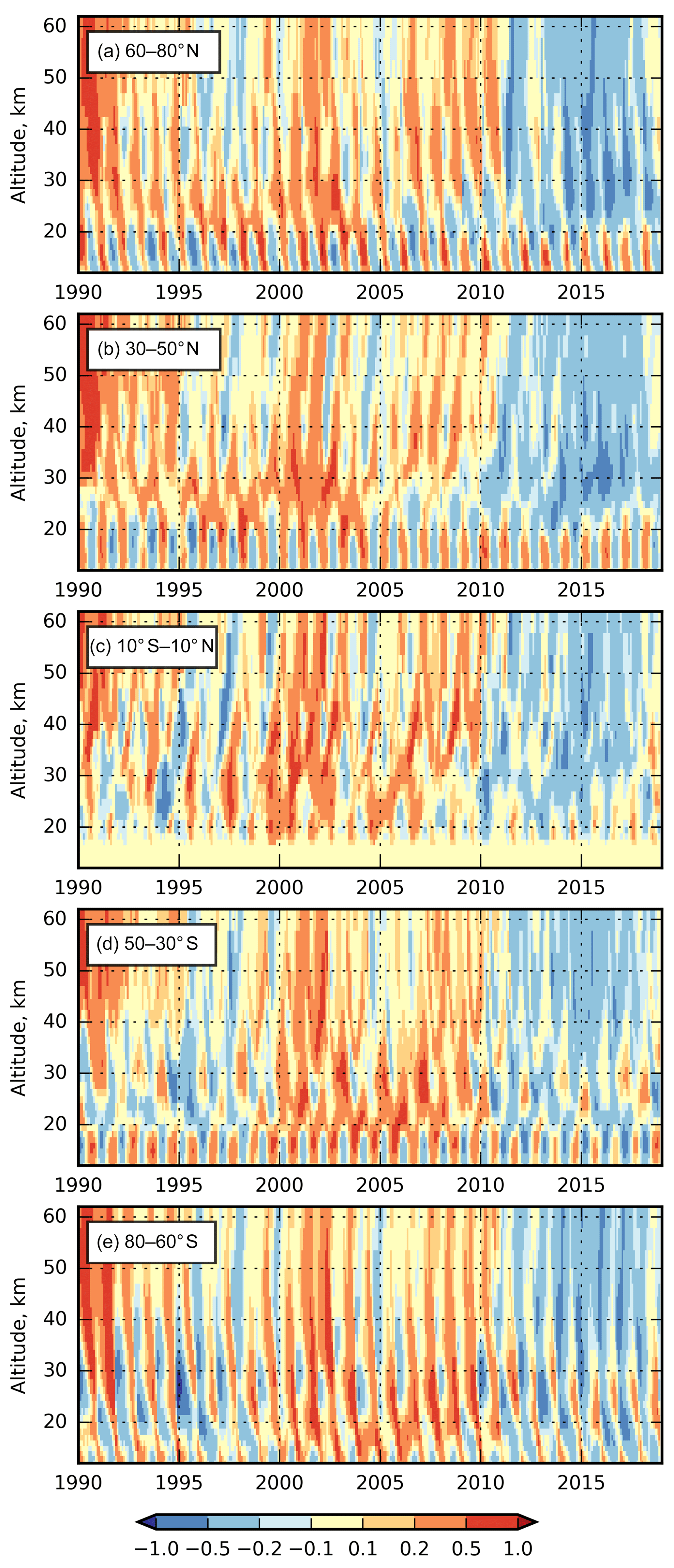
Figure 13Anomaly of the ideal-age AoA (years) for the period of 1990–2018 with respect to the mean AoA.
The zonal-mean vertical profiles of the AoA trends during 2002–2012 are shown in Fig. 12 for five latitudinal belts. The presented variable is a slope of the linear fit of the deseasonalized monthly-mean time series for each tracer, averaged over the corresponding latitudinal belt and the model layer. The fit was made with the ordinary least-squares method. The error bars show 95 % confidence intervals calculated as if a model of linear trend with uncorrelated Gaussian noise was applicable to the time series.
The trends of the apparent AoA for the non-passive SF6 species have a clear increase with height in the upper part of the profiles. Such behaviour agrees well with the AoA trends by Haenel et al. (2015, Fig. 7) obtained from the MIPAS observations. The over-ageing due to the mesospheric depletion of SF6 has been discussed and estimated by Haenel et al. (2015) and Kovács et al. (2017). However, Fig. 12 shows that the mesospheric depletion of SF6 also affects its trend: the over-ageing increases with time. The reason is that depletion is proportional to the SF6 load, which grows with time. This effect has been pointed out and evaluated earlier for N2O by Schoeberl et al. (2000). For SF6, the effect of its loss on the AoA was evaluated by Stiller et al. (2012), who concluded that “in-mixing of mesospheric SF6-depleted air plays a minor role for the assessment of AoA trends”, at least within the framework of their approach (2002–2010, up to 35 km altitude).
The apparent AoA derived with the passive SF6 tracer sf6pass indicates a negative trend of about 0.5 years per decade. The trend is caused by the temporal variation of SF6 emissions. In order to get an unbiased AoA estimate from the passive tracer, one needs the mixing ratio at the surface to be increasing linearly with time. A steady growth of emission rate leads to the faster-than-linear increase of the near-surface mixing ratio and thus a low bias of the AoA. According to the inventory (Levin et al., 2010) used in this study, the SF6 emission rate was growing in 1997–2000 about twice slower than after 2005. Consequently, the negative bias of the apparent AoA has increased resulting in the negative trend of the AoA in the stratosphere.
The AoA trends derived from the ideal-age and passive tracers agree through the whole range of altitudes and latitudes, indicating internal consistency of our simulations. The main common feature of the profiles is the negative tendency of about −0.5 year per decade in the altitude range of 15–30 km with a profile that varies across altitudes. Similar-magnitude trends for the same period were reported by Plöger et al. (2015), who used the same ERA-Interim to simulate AoA. The major difference between the obtained trends is that we have consistently negative trends for both hemispheres, whereas Plöger et al. (2015) indicate a positive trend as a fraction of year per decade in the altitude range of 20–30 km in the Northern Hemisphere and a similar-magnitude negative trend in the Southern Hemisphere. The reason for the discrepancy deserves further investigation. A possible reason for the discrepancy is that Plöger et al. (2015) used diabatic heating rates as vertical velocity, and it is known that the diabatic and kinematic vertical transport is inconsistent in the reanalysis (Abalos et al., 2015).
The trends might be a feature of the non-uniformity of the ERA-Interim dataset, which was produced with assimilation of an inhomogeneous set of the observations. During 2002–2012, the amount of the assimilated data of the upper-air temperatures was an order of magnitude higher than before 2000 and 2 orders of magnitude higher than after 2010 (Dee et al., 2011). It had a clear impact on the patterns of the analysis increments in ERA-Interim and, consequently, on the predicted stratospheric circulation. Due to such inhomogeneities, the quality of trends derived from reanalysis data needs to be verified for each geophysical quantity (Dee et al., 2011). Deducing reliable trends for atmospheric temperature, a quantity that is measurable and extensively assimilated, took a major effort (Simmons et al., 2014). The fact that the AoA is not a directly observable quantity makes the verification of the AoA trends difficult.
To get more insight into the nature of the simulated long-term AoA variability at different altitudes and latitudes, we have plotted the time series of the monthly zonal-mean ideal-age AoA for the same latitude belts as in Fig. 12 over 1990–2018 (Fig. 13). To make the temporal variations more visible, the mean AoA profile for each latitude averaged over the same period was subtracted from the profiles. One can see a clear seasonal variation of the AoA outside the equatorial zone. The variation has opposite phases in the upper and the lower stratosphere. In the altitude range of 20–30 km, where the trends are most pronounced, the temporal variation of the AoA has a ramp structure with more-or-less steady intervals and relatively quick changes. Such a structure is similar to the one shown for the ERA-Interim analysis increments (Dee et al., 2011) and is likely to be caused by temporal inhomogeneities in the assimilated dataset. Therefore, we do not draw any conclusion here on the actual trends of AoA, but we highlight that trends of the apparent AoA are strongly influenced by the selected time interval and by the method of the trends calculation.
The present study has several limitations that deserve specific attention. Forced zero air flux through the domain top at 0.1 hPa caused distortion of the mean transport within the domain and left diffusive transport as the only means for the upper-boundary fluxes of SF6. Secondly, we used prescribed profiles of the eddy diffusivity within the domain, which also affects the results of the simulations. In this section we evaluate the role of these distortions.
6.1 Distortions of air flows
The transport procedure used in this study is done with a “hardtop” diagnostics, forcing zero mass fluxes at the domain top and forced air-mass conservation everywhere within the domain. Since the upper boundary of the domain is at 0.1 hPa, the divergence of the air flow above that level in the meteorological data used to drive the model is compensated by adjusting the divergences within the domain. To evaluate the effect of this adjustment on the mean circulations, we used the new ERA-5 dataset, which has the topmost level at 10−3 hPa. The diagnostic procedure was applied to ERA5 for two sets of vertical layers: the 61 ERA-Interim layers, same as used in the SF6 simulations (hereafter ERA5-cut), and a refined vertical matching the 137 native ERA5 vertical layers (hereafter ERA5). The resulting vertical winds were compared to the ones used in the SF6 simulations: 61 layers diagnosed from ERA-Interim. The seasonal and zonal-mean vertical air-mass fluxes, expressed in units of pascals per day (Pa d−1), for the three cases and two solstice seasons of 2017, are shown in Fig. 14 together with the corresponding layer boundaries.

Figure 14The seasonal and zonal-mean vertical air-mass fluxes diagnosed by SILAM from ERA5 and ERA-Interim fields for 2017 solstice seasons, expressed in terms of vertical velocity ω. Updraughts are red. The vertical-layer boundaries are shown with grey lines.
The wind patterns in ERA5 (Fig. 14a, b, d, e) have finer features than in ERA-Interim due to the higher horizontal resolution. The difference between the ERA5 and ERA5-cut vertical winds is the strongest at the cut-domain top (0.1 hPa, 65 km), where the zero vertical air-mass flux is forced. For both seasons, the disturbances introduced by the cut vertical are minor, except for the summertime poles (South Pole in Fig. 14a, b and North Pole in Fig. 14d, e), where a noticeable disturbance is visible down to 35–40 km altitude. Such systematic disturbances influence the performance of the AoA and the SF6 simulations in the polar stratosphere, and they are a probable reason for the failure of the model to reproduce the SF6 profiles there (see Fig. 6).
The comparison of the mass fluxes for the same vertical levels (panels b vs. c or e vs. f in Fig. 14) shows that the difference between ERA-Interim and ERA5 is noticeably larger than between cut and full vertical of ERA5. Thus we conclude that the distortions introduced by our diagnostic procedure are within the uncertainty of the input meteorological data.
6.2 Top-boundary mass fluxes and eddy diffusion profiles
The used modelling approach replaces the vertical transport through the domain top with the diffusive fluxes for the depleting SF6 and a hard lid for other species. This approach is unlikely to introduce major disturbances into the AoA fields since the AoA is quite uniform close to the domain top. The uncertainty introduced with this approach into the SF6 fields is not straightforward to evaluate due to a major uncertainty in the vertical diffusivity profiles.
As mentioned in Sect. 3.1, the eddy-diffusivity profiles of the C-IFS model from the ERA5 reanalysis (Fig. 1) are clearly unrealistic within and above the stratosphere. They do not exhibit any growth of the eddy diffusivity in the mesosphere either. According to Lindzen (1981) the mean diffusivity due to the breaking gravity waves has an order of magnitude of 102 m2 s−1, whereas the eddy diffusion in ERA5 for that region is below the molecular diffusivity (Fig. 1). On the other hand, if we assume that the mesospheric turbulence results in a diffusivity profile as predicted by Lindzen (1981) (Fig. 1), then such turbulence provides quite rapid exchange of SF6 towards the depletion layers, making the advective vertical transport above ∼50 km negligible. The profiles of Lindzen (1981), however, do not allow for a simple extrapolation below 50 km; therefore, the vertical profiles by Massie and Hunten (1981) (1-Kz) were involved as the ones that are simple to implement and smooth enough to be easily approximated and extrapolated.
The normalized diffusive SF6 mass fluxes above the domain top for the scaled profiles of the eddy diffusivity (Fig. 3) allow for evaluation of the validity of the assumption of neglected regular vertical transport above the domain top. The equivalent vertical air-mass flux due to diffusion at the level of 0.1 hPa (domain top) is , , and it is kg m−2 s−1 for 1-Kz, 0.03-Kz, and 0.001-Kz. These mass fluxes, divided by g, give the vertical velocities of −5, −0.8, and −0.4 Pa d−1. Comparing these values to those shown in Fig. 14 for the level of 65 km, one can see that the diffusive limit is valid for the 1-Kz profile except for the vicinities of the poles. For lower values of the eddy diffusivity, the regular circulation becomes comparable with the diffusion or even exceeds it.
Although the 0.03-Kz profiles gave better agreement with the observations of SF6, this does not indicate that 0.03-Kz profiles are more realistic. This profile is likely to over-mix the lower stratosphere and under-mix the upper stratosphere and the mesosphere. Thus the vertical structure of the eddy diffusivity remains a major source of uncertainty in the modelling approach. Using more realistic vertical diffusion profiles and high-top ERA5 reanalysis is planned for the future studies.
6.3 Notes on the observed SF6 age
There are three main factors responsible for the SF6 age being different from the ideal age: the non-linear growth of tropospheric burden, the gravitational separation, and the mesospheric sink. Here we consider the effects of these factors and corrections to the SF6 observations that can be applied to compensate for the effect of these factors on the resulting AoA.
The correction for the non-linear growth rate introduced by Volk et al. (1997) and used in many subsequent studies is based on a simple analytical model of 1D diffusion with constant diffusivity and exponential distribution of air density. The model was suggested by Hall and Plumb (1994) as an illustration for the concept of the age spectrum. The model spectrum has two parameters: the mean age Γ and the width parameter Δ. In order to use the spectrum for the correction, one has to involve an additional constraint connecting these parameters. Based on a 3D simulation with a general circulation model (GCM), Hall and Plumb (1994) suggested that a constant ratio years can be used throughout the stratosphere. Note that this dimensional parameter, while having proper units originally, appears without units in several subsequent papers (Engel et al., 2002; Stiller et al., 2012). Volk et al. (1997) used the value years for the lower stratosphere based on the results of a more advanced GCM than the one used by Hall and Plumb (1994). With this approach Volk et al. (1997) obtained the difference between the mean age and the lag time (apparent SF6 age). The difference becomes significant for the air older than 3–4 years and approaches 0.5±0.25 years for the oldest (6 years) air, which agrees quite well with the difference between the ideal age and the passive SF6 in our simulations (Fig. 11b, c). The correction for this difference derived from the 1D model has been used to reduce the systematic biases from the SF6-based AoA, though “the global stratosphere is poorly represented by a 1D model” (Waugh and Hall, 2002). The uncertainty of the correction of up to ±0.5 years is systematic, is not guaranteed to be uniform in space or in time, and is likely to affect the trend estimates.
As shown in Sect. 4.1, the biases introduced to the SF6-based AoA by gravitational separation reach a fraction of a year in the upper stratosphere. One could in principle elaborate a correction for gravitational separation; however, the correction would be well within the uncertainty of the correction for the non-linear growth rate, and thus it is probably not worth considering.
The mesospheric sink has the largest impact on the SF6-derived AoA. The effect of the mesospheric sink is clearly visible above 15–20 km at all latitudes (Fig. 11) and leads to a strong over-ageing in the upper layers, especially in the polar areas. The effect of the sink alone can explain the discrepancy between the AoA derived from the MIPAS observations (Haenel et al., 2015) and the AoA from the modelling studies (e.g. Diallo et al., 2012; Brinkop and Jöckel, 2019). Compensating for such over-ageing is hardly possible without detailed modelling of the physical processes including depletion, diffusion, and mean transport. Since the AoA is derived as a difference of the SF6 mixing ratios, whereas depletion introduces multiplicative change to the SF6 abundance, the effect of the sink on apparent SF6 AoA is unsteady in time (Fig. 12).
Once one has a model that is capable of reproducing the processes behind the SF6 depletion, it is natural to validate such a model directly against the available SF6 observations rather than deriving the AoA from the SF6 observations and comparing it against the modelled one. In any case the AoA derived from the SF6 tracer observations with all the corrections can not be considered a purely observed one.
Eulerian simulations of the tropospheric and stratospheric transport of several tracers were performed with the SILAM model driven by the ERA-Interim reanalysis for 1980–2018. The simulations included species representing SF6 under different assumptions: a passive tracer emitted uniformly at the surface and an ideal-age tracer directly comparable to other state-of-the-art CTM simulations of the AoA. To our best knowledge this is the first systematic evaluation of AoA derived from several different tracers within the same multi-decadal simulation, combined with the extensive evaluation against MIPAS and balloon SF6 observations.
Due to the limited vertical coverage and resolution of ERA-Interim in the upper stratosphere, the SILAM simulation domain had a lid at 0.1 hPa, which is below the altitude of the SF6 destruction. In order to perform realistic simulations of SF6 in our setup, the eddy diffusion in the upper stratosphere and lower mesosphere had to be parameterized, along with the mesospheric sink of SF6.
A set of simulations with different parameterizations for the vertical eddy diffusion showed that published profiles derived with no account for advection (e.g. Massie and Hunten, 1981, and references threrin) overestimate the eddy diffusivity. On other hand, the eddy-diffusivity profiles for scalars calculated from the ERA-Interim fields, according to the IFS procedures (ECMWF, 2015) or readily available from the ERA5 reanalysis, appear to be of no relevance for the upper stratosphere, since they fall below the molecular diffusivity. Evaluation of our simulations against satellite and balloon observations indicated that the best agreement between the simulated and observed SF6 mixing ratios within the model domain is achieved for the tabulated eddy-diffusivity profile of Hunten (1975) scaled down with a factor of 30. However, this conclusion is likely to be a feature of the specific model setup. Thus, the question of the importance and magnitude of the eddy diffusivity in the upper stratosphere and lower mesosphere remains open, and the SF6 observations are potentially a good means of its evaluation.
The mesospheric sink of SF6 has a major impact on the mixing ratios above 20 km. The depletion impact is especially strong in the wintertime polar areas due to the descent within a polar vortex. A set of sensitivity tests showed that molecular diffusion and gravitational separation of SF6 are responsible for up to a few percent of further reduction in SF6 mixing ratios in the upper stratosphere.
A good agreement of the simulated SF6 distribution with the MIPAS observations up to the altitudes of 30–35 km and with the available balloon profiles was shown. The standard deviation between the MIPAS and the modelled SF6 mixing ratios is mainly 80 %, controlled by the noise error of the satellite retrievals; i.e. the standard deviation between model and MIPAS is about as large as the error in the satellite data. The results of the comparison also underline the importance of accurate co-location of the modelled and the observed data in terms of space, time, and vertical averaging of the observed data.
The lifetime of SF6 in the atmosphere estimated from the best-performing setup is about 1500 years, which is at the high side of the range of other recent estimates. Our estimate is likely to be biased high due to underrepresented vertical exchange at the domain top due to missing advective transport and the missing effect of breaking gravity waves.
Our simulations were able to reproduce both AoA obtained in other model studies and the apparent SF6 AoA derived from the MIPAS observations. This highlights the role of fast mesospheric destruction of SF6 due to the electron attachment mechanism. Having all tracers within the same simulations, we were able to trace the differences in the estimated AoA to the peculiarities of each tracer. A good agreement between the passive tracer AoA and the ideal-age AoA indicates a consistency of the simulations, since these two methods have opposite sign of sensitivity to errors in the transport scheme.
The mesospheric sink has severe implications for the AoA derived from the SF6. The apparent over-ageing introduced by the sink is large and variable in space and time. Moreover, the over-ageing due to the sink increases as the atmospheric burden of SF6 grows. All this makes SF6 unsuitable to infer AoA above ∼20 km. For a fully passive SF6 tracer, the variable rate of emissions causes deviations from the ideal age, and these deviations can be compensated to some extent. However, correcting the deviations due to the mesospheric sink of SF6 is hardly possible. These deviations appear as long-term trends in the apparent AoA. These trends differ from the trends in the ideal-age AoA and have no direct correspondence to the actual trends in the atmospheric circulation.
Procedures used to derive the AoA from observations of various tracers in the atmosphere are inevitably based on assumptions and idealizations that have limited and often unknown area of applicability. The resulting uncertainties in the AoA are large enough to preclude the use of apparent AoA and its trends for evaluation of changes in atmospheric circulation or for validation of atmospheric models. Observations of the tracers themselves, however, have well quantified uncertainties, so direct comparisons of simulated tracers to the observed ones are a very promising means for the atmospheric model evaluation. AoA in turn is a convenient means for model inter-comparison if a protocol of the AoA derivation is well specified.
The SILAM source code and simulation results are available from Mikhail Sofiev or Rostislav Kouznetsov upon request. The MIPAS observational data are available from Gabriele Stiller upon request. ERA-Interim and ERA5 reanalyses datasets are available from the European Centre for Medium-Range Weather Forecasts https://www.ecmwf.int/en/forecasts/datasets/browse-reanalysis-datasets (Dee et al., 2011; Copernicus Climate Change Service, 2017).
RK designed and performed the simulations and data analyses and prepared the text and illustrations. MS and JV inspired the study, helped with discussions on content and structure of the study, and participated in editing the text. GS provided MIPAS data and wrote sections about MIPAS observations. All authors participated in the final preparation of the text.
The authors declare that they have no conflict of interest.
The authors are grateful to Viktoria Sofieva (Finnish Meteorological Institute) for reading the manuscript and providing useful comments, to Florian Haenel and Michael Kiefer (Karlsruhe Institute of Technology) for technical assistance in handling MIPAS SF6 data, and to four anonymous reviewers whose very instrumental comments helped to substantially improve the paper.
The authors acknowledge the support of the following projects: EU FP7 MarcoPolo (ID: 606953), ESA-ATILA (contract no. 4000105828/12/F/MOS), ASTREX of the Academy of Finland (grant 139126), and the Russian Foundation for Basic Research (project 19-05-01008).
The SF6 and mean age-of-air distributions from MIPAS observations were generated within the project STI 210/5-3 of the CAWSES priority program, funded by the German Research Foundation (DFG) and the project BDCHANGE (01LG1221B), funded by the German Federal Ministry of Education and Research (BMBF) within the ROMIC program.
This research has been supported by the FP7-Space (MARCOPOLO, grant no. 606953), the European Space Agency (ATILA, grant no. 4000105828/12/F/MOS), the Academy of Finland, Luonnontieteiden ja Tekniikan Tutkimuksen Toimikunta (ASTREX, grant no. 139126), the Russian Foundation for Basic Research (project 19-05-01008), the German Research Foundation (CAWSES program, grant no. STI 210/5-3), and the German Federal Ministry of Education and Research (BDCHANGE project of ROMIC program, grant no. 01LG1221B).
This paper was edited by Peter Haynes and reviewed by four anonymous referees.
Abalos, M., Legras, B., Ploeger, F., and Randel, W. J.: Evaluating the advective Brewer-Dobson circulation in three reanalyses for the period 1979–2012, J. Geophys. Res.-Atmos., 120, 7534–7554, https://doi.org/10.1002/2015JD023182, 2015. a
Allen, M., Yung, Y. L., and Waters, J. W.: Vertical transport and photochemistry in the terrestrial mesosphere and lower thermosphere (50–120 km), J. Geophys. Res., 86, 3617–3627, https://doi.org/10.1029/JA086iA05p03617, 1981. a
Andrews, A. E., Boering, K. A., Daube, B. C., Wofsy, S. C., Loewenstein, M., Jost, H., Podolske, J. R., Webster, C. R., Herman, R. L., Scott, D. C., Flesch, G. J., Moyer, E. J., Elkins, J. W., Dutton, G. S., Hurst, D. F., Moore, F. L., Ray, E. A., Romashkin, P. A., and Strahan, S. E.: Mean ages of stratospheric air derived from in situ observations of CO2, CH4, and N2O, J. Geophys. Res., 106, 32295–32314, https://doi.org/10.1029/2001jd000465, 2001. a, b, c
Bhandari, N., Lal, D., and Rama, D.: Stratospheric circulation studies based on natural and artificial radioactive tracer elements, Tellus, 18, 391–406, https://doi.org/10.1111/j.2153-3490.1966.tb00250.x, 1966. a
Boering, K., Wofsy, S., Daube, B., Schneider, H., Loewenstein, M., Podolske, J., and Conway, T.: Stratospheric mean ages and transport rates from observations of carbon dioxide and nitrous oxide, Science, 274, 1340–1343, https://doi.org/10.1126/science.274.5291.1340, 1996. a
Brinkop, S. and Jöckel, P.: ATTILA 4.0: Lagrangian advective and convective transport of passive tracers within the ECHAM5/MESSy (2.53.0) chemistry–climate model, Geosci. Model Dev., 12, 1991–2008, https://doi.org/10.5194/gmd-12-1991-2019, 2019. a, b
Butchart, N., Cionni, I., Eyring, V., Shepherd, T. G., Waugh, D. W., Akiyoshi, H., Austin, J., Brühl, C., Chipperfield, M. P., Cordero, E., Dameris, M., Deckert, R., Dhomse, S., Frith, S. M., Garcia, R. R., Gettelman, A., Giorgetta, M. A., Kinnison, D. E., Li, F., Mancini, E., McLandress, C., Pawson, S., Pitari, G., Plummer, D. A., Rozanov, E., Sassi, F., Scinocca, J. F., Shibata, K., Steil, B., and Tia, W.: Chemistry–Climate Model Simulations of Twenty-First Century Stratospheric Climate and Circulation Changes, J. Climate, 23, 5349–5374, https://doi.org/10.1175/2010jcli3404.1, 2010. a
Copernicus Climate Change Service (C3S): ERA5: Fifth generation of ECMWF atmospheric reanalyses of the global climate, Copernicus Climate Change Service Climate Data Store (CDS), 2018, available at: https://cds.climate.copernicus.eu/cdsapp#!/home (last access: 13 May 2020), 2017. a
Cussler, E. L.: Diffusion: Mass Transfer in Fluid Systems (Cambridge Series in Chemical Engineering), Cambridge University Press, Cambridge UK, 580 pp., 1997. a
Dee, D. P., Uppala, S. M., Simmons, A. J., Berrisford, P., Poli, P., Kobayashi, S., Andrae, U., Balmaseda, M. A., Balsamo, G., Bauer, P., Bechtold, P., Beljaars, A. C. M., van de Berg, L., Bidlot, J., Bormann, N., Delsol, C., Dragani, R., Fuentes, M., Geer, A. J., Haimberger, L., Healy, S. B., Hersbach, H., Hólm, E. V., Isaksen, L., Kållberg, P., Köhler, M., Matricardi, M., McNally, A. P., Monge‐Sanz, B. M., Morcrette, J.‐J., Park, B.‐K., Peubey, C., de Rosnay, P., Tavolato, C., Thépaut, J.‐N., and Vitart, F.: The ERA-Interim reanalysis: configuration and performance of the data assimilation system, Q. J. Roy. Meteorol. Soc., 137, 553–597, https://doi.org/10.1002/qj.828, 2011 (data available at: https://www.ecmwf.int/en/forecasts/datasets/browse-reanalysis-datasets, last access: last access: 13 May 2020). a, b, c, d
Diallo, M., Legras, B., and Chédin, A.: Age of stratospheric air in the ERA-Interim, Atmos. Chem. Phys., 12, 12133–12154, https://doi.org/10.5194/acp-12-12133-2012, 2012. a, b, c, d, e, f
ECMWF: IFS Documentation – Cy41r1, Part 4: Physical processes, Tech. rep., European Center for Medium-range Weather Forecasts, available at: https://www.ecmwf.int/node/9211 (last access: 13 May 2020), 2015. a, b
Eluszkiewicz, J., Hemler, R. S., Mahlman, J. D., Bruhwiler, L., and Takacs, L. L.: Sensitivity of Age-of-Air Calculations to the Choice of Advection Scheme, J. Atmos. Sci., 57, 3185–3201, https://doi.org/10.1175/1520-0469(2000)057<3185:SOAOAC>2.0.CO;2, 2000. a, b
Engel, A., Strunk, M., Müller, M., Haase, H.-P., Poss, C., Levin, I., and Schmidt, U.: Temporal development of total chlorine in the high-latitude stratosphere based on reference distributions of mean age derived from CO2 and SF6, J. Geophys. Res.-Atmos., 107, ACH–1, https://doi.org/10.1029/2001JD000584, 2002. a
Engel, A., Möbius, T., Haase, H.-P., Bönisch, H., Wetter, T., Schmidt, U., Levin, I., Reddmann, T., Oelhaf, H., Wetzel, G., Grunow, K., Huret, N., and Pirre, M.: Observation of mesospheric air inside the arctic stratospheric polar vortex in early 2003, Atmos. Chem. Phys., 6, 267–282, https://doi.org/10.5194/acp-6-267-2006, 2006. a, b
Engel, A., Möbius, T., Bönisch, H., Schmidt, U., Heinz, R., Levin, I., Atlas, E., Aoki, S., Nakazawa, T., Sugawara, S., Moore, F., Hurst, D., Elkins, J., Schauffler, S., Andrews, A., and Boering, K.: Age of stratospheric air unchanged within uncertainties over the past 30 years, Nature Geosci., 2, 28–31, https://doi.org/10.1038/ngeo388, 2009. a, b, c, d, e, f
Engel, A., Rigby, M., Burkholder, J., Fernandez, R., Froidevaux, L., Hall, B., Hossaini, R., Saito, T., Vollmer, M., and Yao, B.: Update on Ozone-Depleting Substances (ODSs) and Other Gases of Interest to the Montreal Protocol, Chapter 1 in Scientific Assessment of Ozone Depletion: 2018, Report 58, World Meteorological Organization, Geneva, Switzerland, available at: https://www.esrl.noaa.gov/csd/assessments/ozone/2018/ (last access: 13 May 2020), 2018. a
England, M. H.: The age of water and ventilation timescales in a global ocean model, J. Phys. Oceanogr., 25, 2756–2777, https://doi.org/10.1175/1520-0485(1995)025<2756:TAOWAV>2.0.CO;2, 1995. a
Garcia, R. R., Randel, W. J., and Kinnison, D. E.: On the determination of age of air trends from atmospheric trace species, J. Atmos. Sci., 68, 139–154, https://doi.org/10.1175/2010JAS3527.1, 2011. a, b, c
Garny, H., Birner, T., Bönisch, H., and Bunzel, F.: The effects of mixing on age of air, J. Geophys. Res.-Atmos., 119, 7015–7034, 2014. a, b
Gavrilov, N. M., Luce, H., Crochet, M., Dalaudier, F., and Fukao, S.: Turbulence parameter estimations from high-resolution balloon temperature measurements of the MUTSI-2000 campaign, Ann. Geophys., 23, 2401–2413, https://doi.org/10.5194/angeo-23-2401-2005, 2005. a
Haenel, F. J., Stiller, G. P., von Clarmann, T., Funke, B., Eckert, E., Glatthor, N., Grabowski, U., Kellmann, S., Kiefer, M., Linden, A., and Reddmann, T.: Reassessment of MIPAS age of air trends and variability, Atmos. Chem. Phys., 15, 13161–13176, https://doi.org/10.5194/acp-15-13161-2015, 2015. a, b, c, d, e, f, g, h
Hall, T. M. and Plumb, R. A.: Age as a diagnostic of stratospheric transport, J. Geophys. Res., 99, 1059–1070, https://doi.org/10.1029/93JD03192, 1994. a, b, c, d, e
Hall, T. M., Waugh, D. W., Boering, K. A., and Plumb, R. A.: Evaluation of transport in stratospheric models, J. Geophys. Res.-Atmos., 104, 18815–18839, 1999. a
Harrison, J. J.: New and improved infrared absorption cross sections for trichlorofluoromethane (CFC-11), Atmos. Meas. Tech., 11, 5827–5836, https://doi.org/10.5194/amt-11-5827-2018, 2018. a
Heimann, M. and Keeling, C. D.: A three-dimensional model of atmospheric CO2 transport based on observed winds: 2. Model description and simulated tracer experiments, pp. 237–275, American Geophysical Union (AGU), https://doi.org/10.1029/GM055p0237, 1989. a, b
Hunten, D. M.: Estimates of Stratospheric Pollution by an Analytic Model, P. Natl. Acad. Sci. USA, 72, 4711–4715, 1975. a, b, c
IPCC: Climate Change 2013: The Physical Science Basis. Contribution of Working Group I to the Fifth Assessment Report of the Intergovernmental Panel on Climate Change, Cambridge University Press, Cambridge, United Kingdom and New York, NY, USA, https://doi.org/10.1017/CBO9781107415324, available at: http://www.climatechange2013.org/ (last access: 13 May 2020), 2013. a
Ishidoya, S., Sugawara, S., Morimoto, S., Aoki, S., and Nakazawa, T.: Gravitational separation of major atmospheric components of nitrogen and oxygen in the stratosphere, Geophys. Res. Lett., 35, L03811, https://doi.org/10.1029/2007gl030456, 2008. a
Ishidoya, S., Sugawara, S., Morimoto, S., Aoki, S., Nakazawa, T., Honda, H., and Murayama, S.: Gravitational separation in the stratosphere – a new indicator of atmospheric circulation, Atmos. Chem. Phys., 13, 8787–8796, https://doi.org/10.5194/acp-13-8787-2013, 2013. a
Jacob, D. J., Prather, M. J., Rasch, P. J., Shia, R.-L., Balkanski, Y. J., Beagley, S. R., Bergmann, D. J., Blackshear, W. T., Brown, M., Chiba, M., Chipperfield, M. P., de Grandpré, J., Dignon, J. E., Feichter, J., Genthon, C., Grose, W. L., Kasibhatla, P. S., Köhler, I., Kritz, M. A., Law, K., Penner, J. E., Ramonet, M., Reeves, C. E., Rotman, D. A., Stockwell, D. Z., Van Velthoven, P. F. J., Verver, G., Wild, O., Yang, H., and Zimmermann, P.: Evaluation and intercomparison of global atmospheric transport models using 222Rn and other short-lived tracers, J. Geophys. Res.-Atmos., 102, 5953–5970, https://doi.org/10.1029/96JD02955, 1997. a
Koch, D. and Rind, D.: Beryllium 10/beryllium 7 as a tracer of stratospheric transport, J. Geophys. Res.-Atmos., 103, 3907–3917, https://doi.org/10.1029/97JD03117, 1998. a
Kovács, T., Feng, W., Totterdill, A., Plane, J. M. C., Dhomse, S., Gómez-Martín, J. C., Stiller, G. P., Haenel, F. J., Smith, C., Forster, P. M., García, R. R., Marsh, D. R., and Chipperfield, M. P.: Determination of the atmospheric lifetime and global warming potential of sulfur hexafluoride using a three-dimensional model, Atmos. Chem. Phys., 17, 883–898, https://doi.org/10.5194/acp-17-883-2017, 2017. a, b, c, d, e, f, g, h, i, j, k
Krol, M., de Bruine, M., Killaars, L., Ouwersloot, H., Pozzer, A., Yin, Y., Chevallier, F., Bousquet, P., Patra, P., Belikov, D., Maksyutov, S., Dhomse, S., Feng, W., and Chipperfield, M. P.: Age of air as a diagnostic for transport timescales in global models, Geosci. Model Dev., 11, 3109–3130, https://doi.org/10.5194/gmd-11-3109-2018, 2018. a, b
Leedham Elvidge, E., Bönisch, H., Brenninkmeijer, C. A. M., Engel, A., Fraser, P. J., Gallacher, E., Langenfelds, R., Mühle, J., Oram, D. E., Ray, E. A., Ridley, A. R., Röckmann, T., Sturges, W. T., Weiss, R. F., and Laube, J. C.: Evaluation of stratospheric age of air from CF4, C2F6, C3F8, CHF3, HFC-125, HFC-227ea and SF6; implications for the calculations of halocarbon lifetimes, fractional release factors and ozone depletion potentials, Atmos. Chem. Phys., 18, 3369–3385, https://doi.org/10.5194/acp-18-3369-2018, 2018. a, b, c
Legras, B., Pisso, I., Berthet, G., and Lefèvre, F.: Variability of the Lagrangian turbulent diffusion in the lower stratosphere, Atmos. Chem. Phys., 5, 1605–1622, https://doi.org/10.5194/acp-5-1605-2005, 2005. a
Levin, I., Naegler, T., Heinz, R., Osusko, D., Cuevas, E., Engel, A., Ilmberger, J., Langenfelds, R. L., Neininger, B., Rohden, C. v., Steele, L. P., Weller, R., Worthy, D. E., and Zimov, S. A.: The global SF6 source inferred from long-term high precision atmospheric measurements and its comparison with emission inventories, Atmos. Chem. Phys., 10, 2655–2662, https://doi.org/10.5194/acp-10-2655-2010, 2010. a, b, c, d
Li, S. and Waugh, D. W.: Sensitivity of mean age and long-lived tracers to transport parameters in a two-dimensional model, J. Geophys. Res.-Atmos., 104, 30559–30569, https://doi.org/10.1029/1999JD900913, 1999. a
Lindzen, R. S.: Turbulence and stress owing to gravity wave and tidal breakdown, J. Geophys. Res.-Oceans, 86, 9707–9714, https://doi.org/10.1029/JC086iC10p09707, 1981. a, b, c, d, e, f
Mange, P.: The theory of molecular diffusion in the atmosphere, J. Geophys. Res., 62, 279–296, 1957. a
Marrero, T. R. and Mason, E. A.: Gaseous diffusion coefficients, J. Phys. Chem. Ref. Data, 1, 3–118, https://doi.org/10.1063/1.3253094, 1972. a, b
Massie, S. T. and Hunten, D. M.: Stratospheric eddy diffusion coefficients from tracer data, J. Geophys. Res., 86, 9859–9867, https://doi.org/10.1029/jc086ic10p09859, 1981. a, b, c
Monge-Sanz, B. M., Chipperfield, M. P., Dee, D. P., Simmons, A. J., and Uppala, S. M.: Improvements in the stratospheric transport achieved by a chemistry transport model with ECMWF (re)analyses: identifying effects and remaining challenges, Q. J. Roy. Meteorol. Soc., 139, 654–673, https://doi.org/10.1002/qj.1996, 2012. a, b, c
Moore, F. L., Elkins, J. W., Ray, E. A., Dutton, G. S., Dunn, R. E., Fahey, D. W., McLaughlin, R. J., Thompson, T. L., Romashkin, P. A., Hurst, D. F., Wamsley, P. R.: Balloonborne in situ gas chromatograph for measurements in the troposphere and stratosphere, J. Geophys. Res.-Atmos., 108, 8330, https://doi.org/10.1029/2001JD000891, 2003. a
Morris, R. A., Miller, T. M., Viggiano, A., Paulson, J. F., Solomon, S., and Reid, G.: Effects of electron and ion reactions on atmospheric lifetimes of fully fluorinated compounds, J. Geophys. Res.-Atmos., 100, 1287–1294, 1995. a
NOAA, NASA, and USAF: U.S. Standard Atmosphere, U.S. Governement Printing Office, Washington D.C., 1976. a, b
Osman, M., Hocking, W., and Tarasick, D.: Parameterization of large-scale turbulent diffusion in the presence of both well-mixed and weakly mixed patchy layers, J. Atmos. Sol.-Terr. Phys., 143–144, 14–36, https://doi.org/10.1016/j.jastp.2016.02.025, 2016. a
Patra, P. K., Lal, S., Subbaraya, B., Jackman, C. H., and Rajaratnam, P.: Observed vertical profile of sulphur hexafluoride (SF6) and its atmospheric applications, J. Geophys. Res.-Atmos., 102, 8855–8859, https://doi.org/10.1029/96JD03503, 1997. a, b, c
Patra, P. K., Houweling, S., Krol, M., Bousquet, P., Belikov, D., Bergmann, D., Bian, H., Cameron-Smith, P., Chipperfield, M. P., Corbin, K., Fortems-Cheiney, A., Fraser, A., Gloor, E., Hess, P., Ito, A., Kawa, S. R., Law, R. M., Loh, Z., Maksyutov, S., Meng, L., Palmer, P. I., Prinn, R. G., Rigby, M., Saito, R., and Wilson, C.: TransCom model simulations of CH4 and related species: linking transport, surface flux and chemical loss with CH4 variability in the troposphere and lower stratosphere, Atmos. Chem. Phys., 11, 12813–12837, https://doi.org/10.5194/acp-11-12813-2011, 2011. a
Pisso, I. and Legras, B.: Turbulent vertical diffusivity in the sub-tropical stratosphere, Atmos. Chem. Phys., 8, 697–707, https://doi.org/10.5194/acp-8-697-2008, 2008. a
Plöger, F., Abalos, M., Birner, T., Konopka, P., Legras, B., Müller, R., and Riese, M.: Quantifying the effects of mixing and residual circulation on trends of stratospheric mean age of air, Geophys. Res. Lett., 42, 2047–2054, https://doi.org/10.1002/2014GL062927, 2015. a, b, c, d
Ravishankara, A., Solomon, S., Turnipseed, A., and Warren, R.: Atmospheric lifetimes of long-lived halogenated species, Science, 259, 194–199, 1993. a, b
Ray, E. A., Moore, F. L., Elkins, J. W., Hurst, D. F., Romashkin, P. A., Dutton, G. S., and Fahey, D. W.: Descent and mixing in the 1999–2000 northern polar vortex inferred from in situ tracer measurements, J. Geophys. Res.-Atmos., 107, 8285, https://doi.org/10.1029/2001JD000961, 2002. a
Ray, E. A., Moore, F. L., Rosenlof, K. H., Davis, S. M., Sweeney, C., Tans, P., Wang, T., Elkins, J. W., Bönisch, H., Engel, A., Sugawara, S., Nakazawa, T., and Aoki, S.: Improving stratospheric transport trend analysis based on SF6 and CO2 measurements, J. Geophys. Res.-Atmos., 119, 14–110, https://doi.org/10.1002/2014JD021802, 2014. a, b
Ray, E. A., Moore, F. L., Elkins, J. W., Rosenlof, K. H., Laube, J. C., Röckmann, T., Marsh, D. R., and Andrews, A. E.: Quantification of the SF6 lifetime based on mesospheric loss measured in the stratospheric polar vortex, J. Geophys. Res.-Atmos., 122, 4626–4638, https://doi.org/10.1002/2016JD026198, 2017. a, b, c, d, e, f, g
Reddmann, T., Ruhnke, R., and Kouker, W.: Three-dimensional model simulations of SF6 with mesospheric chemistry, J. Geophys. Res.-Atmos., 106, 14525–14537, https://doi.org/10.1029/2000JD900700, 2001. a
Remsberg, E. E.: Methane as a diagnostic tracer of changes in the Brewer–Dobson circulation of the stratosphere, Atmos. Chem. Phys., 15, 3739–3754, https://doi.org/10.5194/acp-15-3739-2015, 2015. a
Rigby, M., Mühle, J., Miller, B. R., Prinn, R. G., Krummel, P. B., Steele, L. P., Fraser, P. J., Salameh, P. K., Harth, C. M., Weiss, R. F., Greally, B. R., O'Doherty, S., Simmonds, P. G., Vollmer, M. K., Reimann, S., Kim, J., Kim, K.-R., Wang, H. J., Olivier, J. G. J., Dlugokencky, E. J., Dutton, G. S., Hall, B. D., and Elkins, J. W.: History of atmospheric SF6 from 1973 to 2008, Atmos. Chem. Phys., 10, 10305–10320, https://doi.org/10.5194/acp-10-10305-2010, 2010. a, b, c, d, e
Schoeberl, M. R., Sparling, L. C., Jackman, C. H., and Fleming, E. L.: A Lagrangian view of stratospheric trace gas distributions, J. Geophys. Res.-Atmos., 105, 1537–1552, https://doi.org/10.1029/1999JD900787, 2000. a
Simmons, A., Poli, P., Dee, D., Berrisford, P., Hersbach, H., Kobayashi, S., and Peubey, C.: Estimating low-frequency variability and trends in atmospheric temperature using ERA-Interim, Q. J. Roy. Meteorol. Soc., 140, 329–353, https://doi.org/10.1002/qj.2317, 2014. a
Smith, A. K., Garcia, R. R., Marsh, D. R., and Richter, J. H.: WACCM simulations of the mean circulation and trace species transport in the winter mesosphere, J. Geophys. Res.-Atmos., 116, D20115, https://doi.org/10.1029/2011JD016083, 2011.= a, b
Sofiev, M., Vira, J., Kouznetsov, R., Prank, M., Soares, J., and Genikhovich, E.: Construction of the SILAM Eulerian atmospheric dispersion model based on the advection algorithm of Michael Galperin, Geosci. Model Dev., 8, 3497–3522, https://doi.org/10.5194/gmd-8-3497-2015, 2015. a, b
Stiller, G. P., von Clarmann, T., Höpfner, M., Glatthor, N., Grabowski, U., Kellmann, S., Kleinert, A., Linden, A., Milz, M., Reddmann, T., Steck, T., Fischer, H., Funke, B., López-Puertas, M., and Engel, A.: Global distribution of mean age of stratospheric air from MIPAS SF6 measurements, Atmos. Chem. Phys., 8, 677–695, https://doi.org/10.5194/acp-8-677-2008, 2008. a, b, c, d
Stiller, G. P., von Clarmann, T., Haenel, F., Funke, B., Glatthor, N., Grabowski, U., Kellmann, S., Kiefer, M., Linden, A., Lossow, S., and López-Puertas, M.: Observed temporal evolution of global mean age of stratospheric air for the 2002 to 2010 period, Atmos. Chem. Phys., 12, 3311–3331, https://doi.org/10.5194/acp-12-3311-2012, 2012. a, b, c, d, e, f, g, h, i, j
Strunk, M., Engel, A., Schmidt, U., Volk, C. M., Wetter, T., Levin, I., and Glatzel-Mattheier, H.: CO2 and SF6 as stratospheric age tracers: Consistency and the effect of mesospheric SF6-loss, Geophys. Res. Lett., 27, 341–344, https://doi.org/10.1029/1999GL011044, 2000. a
Sugawara, S., Ishidoya, S., Aoki, S., Morimoto, S., Nakazawa, T., Toyoda, S., Inai, Y., Hasebe, F., Ikeda, C., Honda, H., Goto, D., and Putri, F. A.: Age and gravitational separation of the stratospheric air over Indonesia, Atmos. Chem. Phys., 18, 1819–1833, https://doi.org/10.5194/acp-18-1819-2018, 2018. a
Thiele, G. and Sarmiento, J. L.: Tracer dating and ocean ventilation, J. Geophys. Res.-Oceans, 95, 9377–9391, https://doi.org/10.1029/JC095iC06p09377, 1990. a
Totterdill, A., Kovács, T., Gómez Martín, J. C., Feng, W., and Plane, J. M. C.: Mesospheric Removal of Very Long-Lived Greenhouse Gases SF6 and CFC-115 by Metal Reactions, Lyman-α Photolysis, and Electron Attachment, J. Phys. Chem. A, 119, 2016–2025, https://doi.org/10.1021/jp5123344, 2015. a, b, c, d, e
Varanasi, P., Li, Z., Nemtchinov, V., and Cherukuri, A.: Spectral absorption-coefficient data on HCFC-22 and SF6 for remote-sensing applications, J. Quant. Spectrosc. Ra., 52, 323–332, https://doi.org/10.1016/0022-4073(94)90162-7, 1994. a
Volk, C. M., Elkins, J. W., Fahey, D. W., Dutton, G. S., Gilligan, J. M., Loewenstein, M., Podolske, J. R., Chan, K. R., and Gunson, M. R.: Evaluation of source gas lifetimes from stratospheric observations, J. Geophys. Res.-Atmos., 102, 25543–25564, https://doi.org/10.1029/97JD02215, 1997. a, b, c, d
Waugh, D.: Atmospheric dynamics: The age of stratospheric air, Nature Geosci., 2, 14–16, https://doi.org/10.1038/ngeo397, 2009. a, b, c
Waugh, D. W. and Hall, T. M.: Age of stratospheric air: Theory, observations, and models, Rev. Geophys., 40, 1010, https://doi.org/10.1029/2000rg000101, 2002. a, b, c, d, e, f, g, h, i, j, k, l
Waugh, D. W., Hall, T. M., and Haine, T. W. N.: Relationships among tracer ages, J. Geophys. Res.-Oceans, 108, 3138, https://doi.org/10.1029/2002JC001325, 2003. a
Wilson, R.: Turbulent diffusivity in the free atmosphere inferred from MST radar measurements: a review, Ann. Geophys., 22, 3869–3887, https://doi.org/10.5194/angeo-22-3869-2004, 2004. a