Small-scale structure of thermodynamic phase in Arctic mixed-phase clouds observed by airborne remote sensing during a cold air outbreak and a warm air advection event

Ruiz-Donoso, Elena; Ehrlich, André; Schäfer, Michael; Jäkel, Evelyn; Schemann, Vera; Crewell, Susanne; Mech, Mario; Kulla, Birte Solveig; Kliesch, Leif-Leonard; Neuber, Roland; Wendisch, Manfred

doi:https://doi.org/10.5194/acp-20-5487-2020

Articles | Volume 20, issue 9

https://doi.org/10.5194/acp-20-5487-2020

Special issue:

Arctic mixed-phase clouds as studied during the ACLOUD/PASCAL...

https://doi.org/10.5194/acp-20-5487-2020

Articles | Volume 20, issue 9

Research article

12 May 2020

Research article |

| 12 May 2020

Small-scale structure of thermodynamic phase in Arctic mixed-phase clouds observed by airborne remote sensing during a cold air outbreak and a warm air advection event

Elena Ruiz-Donoso, André Ehrlich, Michael Schäfer, Evelyn Jäkel, Vera Schemann, Susanne Crewell, Mario Mech, Birte Solveig Kulla, Leif-Leonard Kliesch, Roland Neuber, and Manfred Wendisch

Abstract

The combination of downward-looking airborne lidar, radar, microwave, and imaging spectrometer measurements was exploited to characterize the vertical and small-scale (down to 10 m) horizontal distribution of the thermodynamic phase of low-level Arctic mixed-layer clouds. Two cloud cases observed in a cold air outbreak and a warm air advection event observed during the Arctic CLoud Observations Using airborne measurements during polar Day (ACLOUD) campaign were investigated. Both cloud cases exhibited the typical vertical mixed-phase structure with mostly liquid water droplets at cloud top and ice crystals in lower layers. The horizontal, small-scale distribution of the thermodynamic phase as observed during the cold air outbreak is dominated by the liquid water close to the cloud top and shows no indication of ice in lower cloud layers. Contrastingly, the cloud top variability in the case observed during a warm air advection showed some ice in areas of low reflectivity or cloud holes. Radiative transfer simulations considering homogeneous mixtures of liquid water droplets and ice crystals were able to reproduce the horizontal variability in this warm air advection. Large eddy simulations (LESs) were performed to reconstruct the observed cloud properties, which were used subsequently as input for radiative transfer simulations. The LESs of the cloud case observed during the cold air outbreak, with mostly liquid water at cloud top, realistically reproduced the observations. For the warm air advection case, the simulated ice water content (IWC) was systematically lower than the measured IWC. Nevertheless, the LESs revealed the presence of ice particles close to the cloud top and confirmed the observed horizontal variability in the cloud field. It is concluded that the cloud top small-scale horizontal variability is directly linked to changes in the vertical distribution of the cloud thermodynamic phase. Passive satellite-borne imaging spectrometer observations with pixel sizes larger than 100 m miss the small-scale cloud top structures.

How to cite

How to cite.

Dates

Received: 18 Oct 2019 – Discussion started: 25 Oct 2019 – Revised: 25 Mar 2020 – Accepted: 03 Apr 2020 – Published: 12 May 2020

1 Introduction

In the Arctic, low-level stratus and stratocumulus clouds are present around 40 % of the time on annual average (Shupe et al., 2006; Shupe, 2011), and they may persist up to several weeks (Shupe, 2011; Morrison et al., 2012). At least 30 % of these clouds are of mixed-phase type (Mioche et al., 2015). Their radiative properties and lifecycles are determined by the partitioning and the spatial (vertical/horizontal) distribution of liquid water droplets and ice crystals. Therefore, mixed-phase cloud properties are important for the characteristics of the Arctic climate system (Tan and Storelvmo, 2019). They are suspected to play an important role in the accelerated warming relative to lower latitudes observed in the last few decades, a phenomenon known as Arctic amplification (Serreze and Barry, 2011; Wendisch et al., 2017). The microphysical and optical properties of Arctic mixed-phase clouds are determined by a complex network of feedback mechanisms between local and large-scale dynamical and microphysical processes (e.g., Morrison et al., 2012; Mioche et al., 2017). Large-scale advection of air masses across the Arctic predefine their general nature (Pithan et al., 2018). In the case of cold air masses advected from the central Arctic region towards lower latitudes, the cold air transported over the warm ocean surface produces intense shallow convection and characteristic cloud street structures, which may extend over several hundred kilometers. Cold air outbreaks occur all year long, but they are especially frequent in winter (Kolstad et al., 2009; Fletcher et al., 2016). Warm and moist air masses intruding into the Arctic from southern latitudes occur 10 % of the time all year long and are responsible for most of the transport of moisture and heat into the Arctic (Woods et al., 2013; Sedlar and Tjernström, 2017; Pithan et al., 2018). During the northward transport, important air mass transformations take place. The air rapidly cools close to the surface, leading to shallow but strong temperature inversions promoting low-level, persistent clouds (Sedlar and Tjernström, 2017; Tjernström et al., 2015). In these clouds, the vertical motion is driven mainly by radiative cooling at cloud top. As a consequence, convective cells appear in intervals of several kilometers (Shupe et al., 2008; Roesler et al., 2017). On smaller scales of a few hundred meters, the vertical motion is additionally driven by evaporative cooling, associated with entrainment of moist air supplied from upper layers (Mellado, 2017). This entrainment process ensures the formation of liquid water droplets and balances the loss of cloud water by precipitating ice crystals (Korolev, 2007; Shupe et al., 2008; Morrison et al., 2012). Observations by Schäfer et al. (2017, 2018) show that the small-scale horizontal inhomogeneities of updrafts and downdrafts have typical length scales down to 60 m. In downdraft regions, the Wegener–Bergeron–Findeisen process may dominate over the nucleation of liquid water droplets (Korolev and Field, 2008; Korolev et al., 2017), causing the ice crystals to grow at the expense of the liquid water droplets.

Interactions between these processes determine the structure of the cloud, both vertically and horizontally. The cloud thermodynamic phase develops vertically in specific patterns. Most frequently, a liquid-water-dominated layer is observed from which ice crystals precipitate (Shupe et al., 2006; McFarquhar et al., 2007; Ehrlich et al., 2009; Mioche et al., 2015). Spatial differences in the cloud phase vertical distribution can, in turn, occur on horizontal scales down to tens of meters (Korolev and Isaac, 2006; Lawson et al., 2010). Therefore, understanding the radiative properties and temporal evolution of Arctic mixed-phase clouds requires a three-dimensional (3D) characterization of the thermodynamic phase partitioning, which relates the vertical distribution of liquid droplets and ice crystals to the small-scale structures observed close to the cloud top.

The analysis of small-scale microphysical inhomogeneities of Arctic stratus is challenging. Global climate models (GCMs) typically have horizontal and vertical grid sizes of 100 and 1 km, respectively (Tan and Storelvmo, 2016). Global reanalysis products are provided with a horizontal grid that is typically larger than 40 km (Lindsay et al., 2014). This coarse resolution cannot resolve in-cloud microphysical and dynamical processes, such as the updraft and downdraft motions. Therefore, these processes need to be parameterized (Field et al., 2004; Klein et al., 2009). Cloud resolving models (1 km horizontal and 30 m vertical resolution; Luo et al., 2008) and large eddy simulations (LESs, below 100 m horizontal and 15 m vertical resolution; Loewe et al., 2017) resolve small-scale cloud processes and are used to improve the subgrid mixed-phase cloud parameterization of GCMs. In order to evaluate the performance of these high-resolution simulations, adequately resolved observations are needed (Werner et al., 2014; Roesler et al., 2017; Schäfer et al., 2018; Egerer et al., 2019; Neggers et al., 2019; Schemann and Ebell, 2020).

In the past, the observation of the thermodynamic phase transitions associated with small-scale cloud structures down to scales of 10 m was challenging due to limitations of the measurement methods. Passive and active satellite-borne remote sensing techniques have typical resolutions coarser than 250 m (Stephens et al., 2002). Ground-based active cloud remote sensing methods (lidar and radar), with vertical resolution of about 50 m and averaging intervals of 10 s (Kollias et al., 2007; Maahn et al., 2015), mostly point only in zenith direction and thus may miss horizontal inhomogeneities (Marchand et al., 2007). Similarly, airborne in situ measurements of cloud microphysical properties require averaging periods of at least 1 s, integrating over scales of 50 m at a typical flight speed of 50 m s⁻¹ (Mioche et al., 2017), and therefore, potentially mix individual pockets of ice crystals and liquid water droplets. Airborne active radar and lidar measurements also average over along-track distances of about 50 m (1 s at 50 m s⁻¹ flight speed; Stachlewska et al., 2010; Mech et al., 2019). Airborne-imaging remote sensing techniques have the potential to map the cloud top geometry in high spatial resolution. Solar radiation measurements by spectral imagers provide data with an spatial resolution of down to a few meters. Based on this measurement approach, Schäfer et al. (2013) and Bierwirth et al. (2013) retrieved two-dimensional (2D) fields of cloud optical thickness resolving changes in spatial scales smaller than 50 m, which are associated with the evaporation of cloud particles in downdraft regions. For selected cases, Thompson et al. (2016) illustrated the potential of spectral imagers to retrieve 2D fields of cloud thermodynamic phase. The identification of mixed-phase cloud regions, however, was based on the assumption of homogeneously mixed clouds and did not consider the vertical distributions of the ice crystals and liquid water droplets. Due to the passive nature of the imaging spectrometers, the measurements integrate over the entire cloud column, although they are dominated by the cloud properties close to the cloud top (Platnick, 2000). They commonly cannot resolve the clouds vertically. Therefore, to avoid misclassifications, the information about the cloud vertical structure provided by active remote sensing is needed to interpret passive remote sensing measurements of reflected solar radiation.

This study exploits combined passive spectral imaging techniques and active remote sensing measurements (radar and lidar) to characterize the cloud-phase partitioning in the 3D cloud structure. The active remote sensing instruments provide the general vertical stratification of ice particles and liquid water droplets, which is needed to interpret the 2D maps of cloud phase observed by the spectral imager. Two mixed-phase cloud cases detected during the Arctic CLoud Observations Using airborne measurements during polar Day (ACLOUD) campaign are chosen to demonstrate this instrument synergy (Wendisch et al., 2019). Section 2 introduces the instrumentation, the retrieval approach to derive 2D maps of cloud phase, and the LESs. The two case studies are presented in Sect. 3, including a discussion of the impact of the cloud vertical structure on the cloud phase retrieval. The observation are compared to LESs in Sect. 4. The information loss due to the smoothing of the fine-scale cloud structures to the typical geometry obtained by satellite-borne remote sensing is quantified in Sect. 5.

2 Methods

2.1 Observations

The ACLOUD campaign was performed to improve the understanding of the role of Arctic low and midlevel clouds in Arctic amplification; it took place in the vicinity of the Svalbard archipelago in May and June 2017 (Wendisch et al., 2019; Ehrlich et al., 2019). During ACLOUD, active and passive remote sensing instruments and in situ probes were operated on the research aircraft Polar 5 and Polar 6 of the Alfred Wegener Institute, Helmholtz Centre for Polar and Marine Research (AWI; Wesche et al., 2016). Among the in situ probes installed on Polar 6, the Small Ice Detector (SID-3, Vochezer et al., 2016) provides the particle size distribution of hydrometeors with sizes between 5 and 45 µm. The passive remote sensing equipment installed on Polar 5 included, among others, the AISA Hawk spectral imager (Pu, 2017). The downward-viewing pushbroom sensor of AISA Hawk is aligned across-track to measure 2D fields of upward radiance ( $I_{λ}^{↑}$ ) reflected by the cloud and surface. Considering uncertainties due to the calibration and noise in the measured signal, the uncertainty in the measured radiance is estimated to be approximately 6 % (Schäfer et al., 2013). With 384 across-track pixels, a 36^∘ field of view (FOV) and a typical vertical distance between aircraft and cloud top of 1 km, AISA Hawk samples with a spatial resolution of roughly 2 m. At this resolution, horizontal photon transport needs to be taken into account. The AISA Hawk measurements have been corrected from this effect using the deconvolution algorithm introduced in Appendix A. Each pixel contains spectral measurements between 930 and 2550 nm wavelength in 288 channels with an average spectral resolution (full width at half maximum, FWHM) of about 10 nm. More details on the calibration of AISA Hawk and the data processing are presented by Ehrlich et al. (2019). Two-dimensional fields of spectral cloud top reflectivity (R_λ) are obtained by combining reflected radiance fields, detected by AISA Hawk, with simultaneous measurements of the downward spectral irradiance ( $F_{λ}^{↓}$ ) obtained by the Spectral Modular Airborne Radiation measurement sysTem (SMART; Wendisch et al., 2001; Ehrlich et al., 2019) as follows:

\begin{matrix} (1) & R_{λ} = π \cdot \frac{I_{λ}^{↑}}{F_{λ}^{↓}} . \end{matrix}

The cloud top reflectivity R_λ in the spectral range between λ_a=1550 nm and λ_b=1700 nm, characterized by the different absorption features of liquid water and ice, is used to discriminate the cloud thermodynamic phase (Pilewskie and Twomey, 1987; Chylek and Borel, 2004; Jäkel et al., 2013; Thompson et al., 2016). The spectral differences in the cloud top reflectivity of pure liquid and pure ice clouds are illustrated in Fig. 1. To identify the cloud phase, Ehrlich et al. (2008 a) defined the slope phase index (ℐ_s), which quantifies the spectral slope of the cloud top reflectivity in this spectral region and is sensitive to the amount of ice crystals and liquid water droplets close to cloud top:

\begin{matrix} (2) & I_{s} = 100 \cdot \frac{(λ_{b} - λ_{a})}{R_{1640}} {(\frac{d R_{λ}}{d λ})}_{[λ_{a}, λ_{b}]} . \end{matrix}

A threshold value for the slope phase index of 20 discriminates between pure liquid water (ℐ_s<20) and pure ice or mixed-phase (ℐ_s>20) close to cloud top (Ehrlich et al., 2009). By applying Eq. (2) to the AISA Hawk measurements, fields of ℐ_s are generated, which resolve the horizontal distribution of the thermodynamic phase of the cloud uppermost 200 m layer, typically corresponding to an in-cloud optical depth of about 5 (Platnick, 2000; Ehrlich, 2009; Miller et al., 2014).

The vertical distribution of the cloud thermodynamic phase is retrieved from measurements by the Microwave Radar/radiometer for Arctic Clouds (MiRAC; Mech et al., 2019) and the Airborne Mobile Aerosol Lidar (AMALi; Stachlewska et al., 2010) deployed in parallel with the AISA Hawk sensor on board Polar 5. The radar reflectivity is proportional to the sixth power of the particle size distribution and, thus, is most sensitive to large particles, such as ice crystals (Hogan and O'Conner, 2004; Shupe, 2007; Kalesse et al., 2016). Therefore, it is used as an indicator of the vertical location of large ice crystals in mixed-phase clouds. In contrast, the AMALi backscatter signal is strongly attenuated by high concentrations of small particles and, thus, identifies the location of small supercooled liquid water droplets close to the cloud top in mixed-phase clouds.

2.2 Radiative transfer modeling

Radiative transfer simulations are employed to interpret the horizontal structure of the slope phase index and to retrieve 2D fields of cloud optical thickness (τ) and effective radius (r_eff). They were performed with the Library for Radiative transfer (libRadtran) code (Mayer and Kylling, 2005; Emde et al., 2016). The simulations applied the radiative transfer solver FDISORT2 (Discrete Ordinate Radiative Transfer) introduced by Stamnes et al. (2000). The standard sub-Arctic summer atmospheric profile provided by libRadtran was employed, together with temperature and water vapor profiles measured by dropsondes released during the respective flights close to the measurement sites. A maritime aerosol type and the surface albedo of open ocean were selected (Shettle, 1990). The solar zenith angle (SZA) was adjusted to the location and time of each specific measurement. The simulations of liquid water clouds assumed the validity of Mie theory, whereas those including ice clouds assumed columnar ice crystals and applied the “Hey” parameterization, based on Yang et al. (2000) to convert microphysical into optical properties. Regarding the phase index, Ehrlich et al. (2008 a, b) found that the influence of the ice crystal shape is of minor importance compared to the impact of the particle size, which was confirmed by additional simulations considering different ice crystal habits (not shown here). Hence, the assumption of columns is sufficient to account for the nonsphericity effects of the ice crystals.

In a first step, extending the work of Bierwirth et al. (2013) and Schäfer et al. (2013) to the near-infrared spectral range, the spectral cloud top reflectivity fields measured by AISA Hawk were used to retrieve fields of optical thickness and effective radius. For this purpose, the reflectivity R₁₂₄₀ at a wavelength of 1240 nm (scattering dominated), sensitive to the cloud optical thickness, is combined with R₁₆₂₅ at a wavelength of 1625 nm, where absorption of solar radiation dominates and is influenced mainly by the particle size (Nakajima and King, 1990). The location of these wavelengths in the cloud top reflectivity spectrum are shown in Fig. 1. To reduce the retrieval uncertainties, the radiance ratio approach by Werner et al. (2013) was applied. Look-up tables considering the sensor viewing geometry of every pixel of AISA Hawk are simulated for various combinations of cloud optical thickness and effective radius. For the simulations, pure liquid water clouds are assumed. Therefore, in the case of mixed-phase clouds, the retrieved values of optical thickness and effective radius might be biased. However, since Arctic low-level mixed-phase clouds are typically topped by a liquid-water layer (Shupe et al., 2006; McFarquhar et al., 2007), the associated uncertainties are expected to be lower than the variability within the cloud field.

The retrieved optical thickness and effective radius, assuming a plane-parallel 1D radiative transfer model, are affected by 3D radiative effects (Zinner and Mayer, 2006; Marshak et al., 2006). While the 3D nature of the cloud structures will cause an overestimation of the optical thickness in the brightly illuminated areas, the effective radius is overestimated in the shadowed regions. Horváth et al. (2014) showed that, due to their opposite sign, the 3D bias of retrieved optical thickness and effective radius partially cancel when calculating the liquid water path (LWP). Therefore, the retrieved fields of τ and r_eff are converted into fields of LWP using the relation by Kokhanovsky (2004):

\begin{matrix} (3) & LWP = \frac{2}{3} \cdot ρ \cdot τ \cdot r_{eff} . \end{matrix}

As it was the case for the retrieved τ and r_eff, this conversion assumes liquid water clouds with a homogeneously mixed vertically constant profile. Considering a homogeneous vertical profile may result in inaccuracies even for pure liquid water clouds (Zhou et al., 2016). Mixed-phase clouds, in addition, violate the pure-phase assumption. The presence of ice crystals introduces a significant error in the calculated LWP, which reaches values well above the typical values observed in Arctic pure liquid water clouds. Past observations show that the LWP of typical Arctic boundary-layer clouds is in the range of 30–50 g m⁻² and rarely exceeds 100 g m⁻² (Shupe et al., 2006; Mioche et al., 2017; Nomokonova et al., 2019; Gierens et al., 2020). Appendix A analyzes the different impact of shades and inhomogeneous thermodynamic phase distributions in the retrieved LWP. In this paper, unrealistically high retrieved LWP values are used to identify mixed-phase clouds.

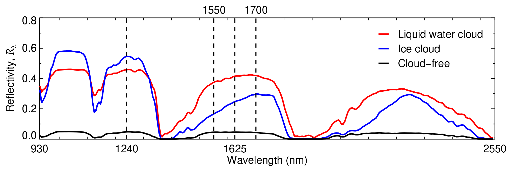
https://www.atmos-chem-phys.net/20/5487/2020/acp-20-5487-2020-f01

Figure 1Reflectivity spectra of a pure liquid water cloud and a pure ice cloud of optical thickness 12 compared with a clear-sky spectrum in the wavelength range measured by AISA Hawk. The vertical dashed lines indicate the wavelengths needed to calculate the slope phase index (1550–1700 nm) and to retrieve the cloud optical thickness (1240 nm) and effective radius (1625 nm).

Download

2.3 Large eddy simulation (LES)

Simulations using the ICOsahedral Non‐hydrostatic atmosphere model (ICON), operated in its large eddy model (LEM) configuration (Heinze et al., 2017; Dipankar et al., 2015), provide a quantitative view into the cloud vertical structure. The simulated cloud vertical profiles were used as input for radiative transfer simulations to analyze the impact of different vertical distributions of the cloud thermodynamic phase on the cloud top horizontal variability.

ICON-LEM simulations were forced by initial and lateral boundary conditions from the European Centre for Medium-Range Weather Forecasts (ECMWF) Integrated Forecast System (IFS; Gregory et al., 2010). The simulations were preformed in a one-way nested setup with a 600 m spatial resolution at the outermost domain, followed by 300 m resolution and an inner triangular nest of 150 m resolution. This inner nest was equivalent to a square grid of 100 m horizontal resolution, which is about 1 order of magnitude coarser than the observations by AISA Hawk. Simulations with finer horizontal resolution were not reasonable due to the high computational time. In the vertical direction, 150 height levels were simulated. In the ICON-LEM simulations the two-moment, mixed-phase bulk microphysical parameterization by Seifert and Beheng (2006) was applied. It provided vertical profiles of liquid and ice mass mixing ratios, r_w and r_i, cloud droplets and ice crystal number concentrations, N_w and N_i, air temperature T, and pressure p. The mass mixing ratio and the number concentration profiles take into consideration both the non-precipitating (cloud water and cloud ice) and the precipitating (rain, snow, graupel, and hail) hydrometeors. They have been used to convert the r_w and r_i into liquid water content and ice water content (LWC and IWC), as required by the radiative transfer model as follows:

\begin{matrix} (4) & LWC (z) = r_{w} (z) \cdot \frac{p (z)}{R \cdot T (z)}, IWC (z) = r_{i} (z) \cdot \frac{p (z)}{R \cdot T (z)}, \end{matrix}

with R=287.06 $J {kg}^{- 1} K^{- 1}$ the specific gas constant for dry air and z the altitude. For the spherical liquid water droplets, vertical profiles of droplet effective radius are obtained by (Martin et al., 1994; Kostka et al., 2014):

\begin{matrix} (5) & r_{eff,liquid} (z) = {[\frac{3 \cdot r_{w} (z)}{4 \cdot π \cdot ρ_{w} \cdot N_{w} (z)}]}^{1 / 3}, \end{matrix}

where ρ_w is the density of the liquid water. For the nonspherical ice crystals, the median mass diameter D_m,ice of the particle size distribution (PSD) of cloud ice represented by the generalized Γ distribution described by Seifert and Beheng (2006), used by ICON-LEM, is calculated as

\begin{matrix} (6) & D_{m, ice} (z) = a \cdot {[\frac{r_{i} (z)}{N_{i} (z)}]}^{b}, \end{matrix}

with $a = 0.206 \times 10^{- 6}$ m kg^−b and b=0.302. The radiative properties of ice crystals were parameterized using the effective radius r_eff,ice. To convert the median particle size into radius r_eff,ice, the measurement-based relationship between D_m,ice and the effective diameter, D_eff,ice, of columnar ice crystals introduced by Baum et al. (2005) and Baum et al. (2014) was used.

https://www.atmos-chem-phys.net/20/5487/2020/acp-20-5487-2020-f02

Figure 2MODIS true color images from the NASA Worldview application (https://worldview.earthdata.nasa.gov, last access: 5 October 2019) on (a) 25 May 2017 during a cold air outbreak and on (c) 2 June 2017 during a warm air advection. Zooms into the regions delimited by black squares are shown in (b) and (c). The measurements location (79.5^∘ N, 9.5^∘ E on 25 May and 79.2^∘ N, 10.7^∘ E on 2 June) is indicated by the green section of the flight track of Polar 5 (orange). The areas extracted from the LESs are indicated by the dashed red rectangle. The dashed-dotted blue on 2 June line indicates the location of the SID-3 measurements.

https://www.atmos-chem-phys.net/20/5487/2020/acp-20-5487-2020-f03

Figure 3Combination of MiRAC radar reflectivity (color range between blue and red) and AMALi backscatter ratio (colors between white and black) as measured on (a) 25 May 2017 during a cold air outbreak and on (b) 2 June 2017 during a warm air advection. AMALi's lidar backscatter ratio is highly sensitive to the liquid droplets and shows the liquid top layer in both clouds. MiRAC's radar reflectivity is dominated by larger particles and indicate regions with ice crystals. The radar signal below an altitude of 150 m is heavily influenced by ground clutter and cannot interpreted for cloud studies.

Download

3 Results of measurements and radiative transfer simulations

The ACLOUD campaign was classified by Knudsen et al. (2018) into a cold (23 May–29 May) period, a warm (30 May–12 June) period, and a neutral (13 June–26 June) period . During the cold period, the Svalbard region was affected by a northerly cold air outbreak, which led to the development of low-level clouds over the warm open ocean. Over the Fram Strait, these clouds organized in a roll convective structure, forming typical cloud streets. During the warm period, a high pressure system south of Svalbard advected warm air from the south over the archipelago, leading to the development of a low-level, optically thick, and homogeneous stratocumulus. Cold air outbreaks and warm air advections are phenomena often affecting the Arctic regions (Pithan et al., 2018; Sedlar and Tjernström, 2017; Woods et al., 2013; Kolstad et al., 2009; Fletcher et al., 2016). The occurrence of both situations during the ACLOUD campaign make it an ideal test bed to contrast the characteristics of the clouds occurring under each situation. Two cloud cases observed on 25 May, during the cold air outbreak, and on 2 June 2017, during the warm air advection, were analyzed in detail. Figure 2 displays the corresponding MODerate resolution Imaging Spectroradiometer (MODIS) true color images showing the clouds on both days.

Figure 3 illustrates the combined measurements of MiRAC and AMALi for the 1 min sequence acquired over open ocean for the two cloud cases. The combination of measurements is interpreted qualitatively to gain an insight into the clouds vertical structure. In both cases, the liquid cloud top is well identified by the strong backscatter of the lidar signal, defined as in Langenbach et al. (2019) and highly sensitive to liquid droplets. Whereas on 25 May the liquid layer is geometrically thicker, the lidar reaches the surface, which indicates a cloud optical thickness of less than 3–4 (McGill et al., 2004). On 2 June, the lidar could not penetrate the cloud. The stronger attenuation of the lidar signal, i.e., the rapid decrease in the lidar backscatter, hints at larger amounts of liquid than on 25 May. In contrast, the radar signal is dominated by larger particles, and higher radar reflectivity values commonly indicate higher concentrations of ice crystals. The combination of the radar and lidar signals helps to identify differences in the vertical structure of both clouds. The cloud on 25 May, showing a high radar reflectivity, contains very likely precipitating large ice crystals. In this case, some regions of the cloud are characterized by a large radar reflectivity at cloud top, shown by the overlapping radar and lidar signals in Fig. 3a, which hints at the presence of large particles in high cloud layers. Vertical separation between the signals of both instruments, such as occurring around 09:01:47 UTC, indicate regions where small liquid droplets dominate the cloud top, detected by the lidar but not by the radar. In these regions, the radar observes large particles, likely ice crystals, around 100 m below the cloud top which precipitate down to the surface. On 2 June (Fig. 3b), the radar reflectivity is weaker than on 25 May and shows no evidence of precipitation reaching the surface. The weaker radar reflectivity may be attributed either to smaller ice crystals or to a reduced particle concentration. However, the continuous overlap between the lidar and the radar signals in Fig. 3 indicates the presence of large particles right below the cloud top. These differences in the vertical structures of the two cloud cases need to be considered when interpreting the 2D horizontal fields of the slope phase index retrieved by AISA Hawk, which is most sensitive to the cloud top layer.

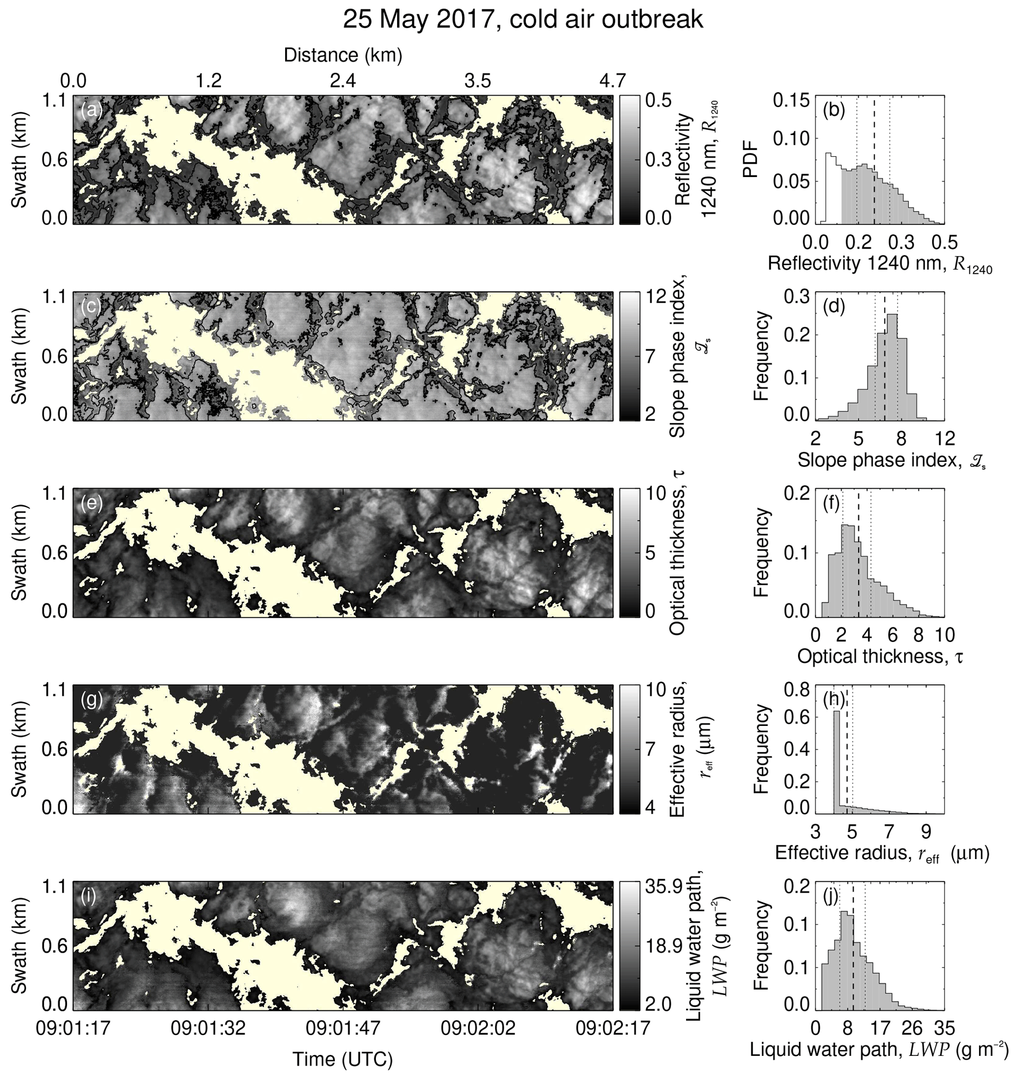
https://www.atmos-chem-phys.net/20/5487/2020/acp-20-5487-2020-f04

Figure 4AISA Hawk measurement on 25 May 2017. (a) Cloud top reflectivity, (c) slope phase index, (e) retrieved optical thickness, (g) retrieved effective radius, and (i) liquid water path. The overlaid contours in (a) and (c) separate the cloud central regions from the cloud edges. The frequency of occurrence histograms are displayed on the corresponding righthand panels (b), (d), (f), (h), and (j). Data classified as cloud-free are shown by the non-colored histogram in (b). Dashed lines indicates the mean value of each field, and the dotted lines show the corresponding 25th and 75th percentiles.

3.1 Cold air outbreak

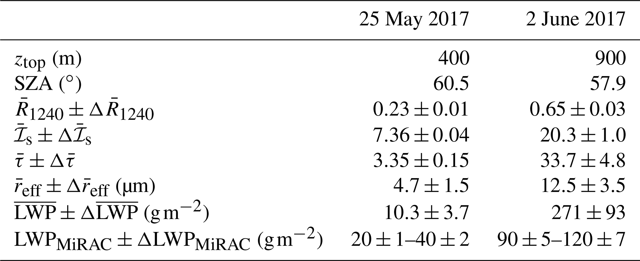
Figure 4 presents a sequence of AISA Hawk measurements and retrieved horizontal fields of cloud properties (R₁₂₄₀, ℐ_s, τ, r_eff, and LWP) together with corresponding histograms. They were observed during the cold air outbreak on 25 May 2017 in the flight section shown in Fig. 2a and b, simultaneously with the MiRAC and AMALi observations in Fig. 3a. Mean values and associated uncertainty in the cloud properties are summarized in Table 1. The measurements present 1 min of data acquired at 09:01 UTC with a SZA of 60.5^∘ at a flight altitude of 2.8 km. The average cloud top was located at 400 m above sea level. The observed cloud scene covers an area of 1.1 km×4.7 km with an average pixel size of 3.9 m×2.6 m. Figure 4a shows the cloud top reflectivity field at 1240 nm wavelength, R₁₂₄₀, and a corresponding histogram in Fig. 4b. Due to the broken character of the cloud field, a cloud mask has been applied prior to the retrieval of cloud properties. Based on radiative transfer simulations, a threshold of R₁₂₄₀=0.1, roughly corresponding to a LWP of 2 g m⁻², was chosen to discriminate between cloudy and cloud-free areas. Regions with R₁₂₄₀<0.1 were classified as cloud-free and have been excluded from further analysis.

The slope phase index ℐ_s, presented in Fig. 4c and d, shows a maximum value of 12.6, which is characteristic for pure liquid water clouds. This seems to disagree with the lidar and radar observations (Fig. 3), which indicated a mixed-phase cloud, and demonstrates the higher sensitivity of the phase index to the thermodynamic phase of the top most layer. Similarly, the LWP (Fig. 4i), calculated from τ (Fig. 4e) and r_eff (Fig. 4g) using Eq. (3), increases towards the cloud core centers, as it is typical for pure liquid water clouds. These areas visually identify updraft regions where enhanced condensation occurs due to adiabatic cooling (Gerber et al., 2005).

Although ℐ_s is always below the threshold of pure ice clouds, the cloud field presents significant small-scale variability that might be related to spatial changes in the thermodynamic phase distribution. To quantify if regions of enhanced ℐ_s are correlated with areas of precipitating ice crystals, as observed by MiRAC, the cloud edges were separated from the central cloud regions. All pixels below the 25th percentile of R₁₂₄₀ and of ℐ_s are defined as cloud edges. All other areas are considered to be cloud core center regions. The separated measurements were compared to 1D radiative transfer simulations adapted to the measurement situation. In Fig. 5, the measured slope phase index is presented as a function of the cloud top reflectivity, together with simulations assuming pure-phase (either liquid or ice) clouds of known particle sizes and liquid/ice water paths (LWPs, IWPs). This sensitivity study shows the spread of ℐ_s as a function of the cloud thermodynamic phase, the cloud optical thickness (or LWP and IWP), and the cloud particle size. An accurate phase classification cannot rely on a fixed ℐ_s threshold value and depends on the combined ℐ_s and R₁₂₄₀ values. Figure 5 reveals that the observed ℐ_s and R₁₂₄₀ range within simulated values covered by pure liquid water clouds. The spatiotemporal changes in the measurement (color code in Fig. 5) indicate that a transition from cloud edge into cloud core follows lines with increasing LWP and slightly increasing particle sizes. This pattern can be explained by the dynamical and microphysical processes in cloud cores where ascending air condenses and cloud droplets grow with altitude, leading to a higher LWP. Hence, the small-scale variability in ℐ_s observed on 25 May 2017 can be interpreted as the natural variability of the cloud top liquid layer. Compared to the radar observations, the passive reflectivity measurements are insensitive to the precipitating ice crystals.

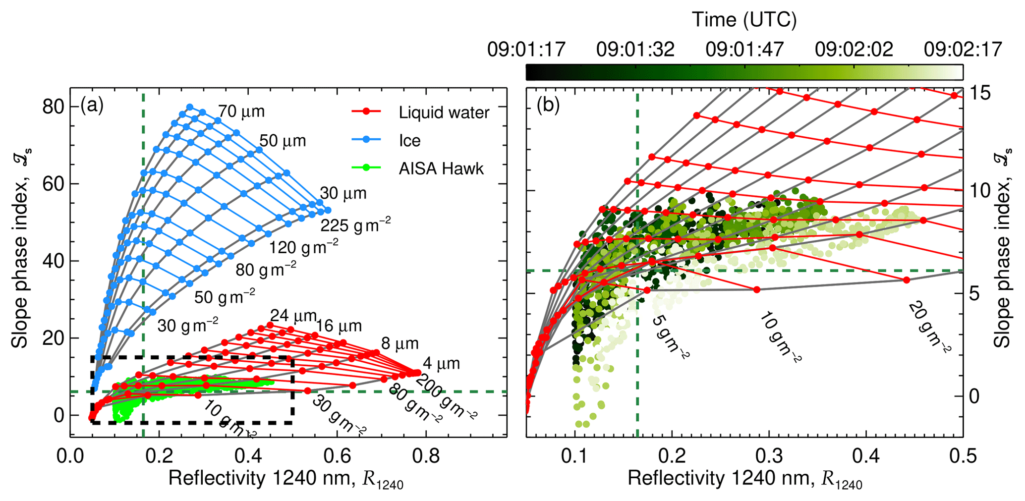
https://www.atmos-chem-phys.net/20/5487/2020/acp-20-5487-2020-f05

Figure 5(a) ℐ_s measured on 25 May 2017 presented as a function of R₁₂₄₀ (green dots). The dashed lines indicate the 25th percentile of R₁₂₄₀ and ℐ_s. The two grids represent radiative transfer simulations for a range of pure liquid (red) and pure ice (blue) clouds. The liquid water clouds cover droplets with r_eff between 4 and 24 µm and LWP between 1 and 250 g m⁻². The ice clouds are simulated for columnar ice crystals with r_eff between 28 and 90 µm and IWP between 1 and 250 g m⁻². A SZA of 60.5^∘ was considered. (b) Zoom of the area highlighted by a dashed rectangle in (a). Color-coded is the acquisition time of the measurements illustrating changes along the flight path.

Download

Table 1Average value and uncertainty (Δ) in the cloud top properties derived from the measurements of AISA Hawk on 25 May and on 2 June. Independent estimations of the LWP range by the passive 89 GHz channel of MiRAC are also included.

Download Print Version | Download XLSX

3.2 Warm air advection

3.2.1 2D horizontal fields

A sequence of R₁₂₄₀ and retrieved cloud properties (ℐ_s, τ, r_eff, and LWP) observed in the ACLOUD warm period on 2 June 2017 is shown in Fig. 6 for the flight section of Fig. 3b. Table 1 presents the mean values and associated uncertainty in the presented cloud properties. The 1 min sequence starts at 09:45 UTC, when the SZA was of about 57.9^∘. The lidar observations indicated that the cloud top of the low-level stratocumulus was located at 900 m above sea level. Hence, for a flight altitude of 2.9 km, the field covers a cloud area of 0.9 km×5.6 km with an average pixel size of 3.1 m×4.7 m. The cloud top reflectivity at 1240 nm wavelength, displayed in Fig. 6a, shows a rather horizontally uniform cloud layer compared to the measurements collected on 25 May 2017 (Case I). The cloud mask (R₁₂₄₀>0.1) reveals a 100 % cloud coverage for this scene. The slope phase index, presented in Fig. 6c, is higher compared to the cloud case presented in Fig. 4 and ranges between 14.9 and 36.5. Applying the common threshold of 20 would classify larger regions of the observed clouds as pure ice or mixed-phase. However, the LWP (Fig. 6i) shows significant variability over the entire cloud field, which may be related to the spatial distribution of the thermodynamic phase. The comparison of the relation between ℐ_s and R₁₂₄₀ with simulations assuming pure-phase clouds is shown in Fig. 7. The simulations reveal that the measurements do not fall in the range of the grid simulated for pure ice clouds, which would typically have higher values of slope phase index than observed. The measurements rather resemble the simulations of pure liquid water clouds. However, the field and histogram of LWP (Fig. 6i and j) show an average value of 270 g m⁻² with the 25 % percentile at 250 g m⁻². Such high LWP values have rarely been observed in Arctic low-level clouds, which typically range between 30 and 50 g m⁻² and rarely exceed 100 g m⁻² (Shupe et al., 2005; de Boer et al., 2009; Mioche et al., 2017; Nomokonova et al., 2019; Gierens et al., 2020). The measurements by the passive 89 GHz channel of the microwave radiometer of MiRAC were used to estimate the LWP independently (see Appendix B for retrieval description and uncertainty assessment). The values between 90 and 120 g m⁻² indicate that the LWP retrieval using the AISA Hawk measurements is strongly overestimated likely due to the presence of ice crystals close to cloud top (compare Fig. 3). This is supported by the rather high optical thickness and particle sizes retrieved from AISA Hawk measurements, shown in Fig. 6e–h. As the retrieval assumes liquid droplets, the presence of ice crystals, which are typically larger and strongly absorb radiation at 1625 nm wavelength, bias the retrieval of both quantities towards higher values (Riedi et al., 2010). The particle size distribution observed by the SID-3 (Schnaiter and Järvinen, 2019) deployed in Polar 6 between 09:25 and 09:35 UTC in the vicinity of the AISA Hawk measurements (Fig. 2) revealed that, for the observed cloud, the particles at cloud top present effective radii of approximately 10 µm. Overall, 75 % of the AISA Hawk measurements on 2 June retrieved an effective radii larger than this value (Fig. 6g and h). The small-scale variability in the cloud properties shows that the largest deviation in the retrieved r_eff and LWP with respect to the external measurements occurs in areas of low reflectivity (below the 25th percentile of R₁₂₄₀) and high slope phase index values (above the 75th percentile of ℐ_s). These areas indicate cloud holes, where the vertical velocity is likely downwards, and the condensation of liquid droplets is reduced, which increases the fraction of ice crystals. Although the theory predicts low values of LWP and r_eff in these regions (Gerber et al., 2005, 2013), the high ice fraction leads to the strong overestimation of LWP compared to the microwave retrieval. In contrast to the pattern observed on 25 May 2017, the higher ice fraction in the edges of the cloud holes causes the slope phase index to decrease with increasing cloud top reflectivity.

https://www.atmos-chem-phys.net/20/5487/2020/acp-20-5487-2020-f06

Figure 6AISA Hawk measurement on 2 June 2017. (a) Cloud top reflectivity, (c) slope phase index, (e) retrieved optical thickness, (g) retrieved effective radius, (i) and liquid water path. The overlaid contours in (a) and (c) separate the cloud central regions from the cloud edges. The frequency of occurrence histograms are displayed on the corresponding righthand panels (b), (d), (f), (h), and (j). The dashed line indicates the mean value, and the dotted lines show its 25th and 75th percentiles.

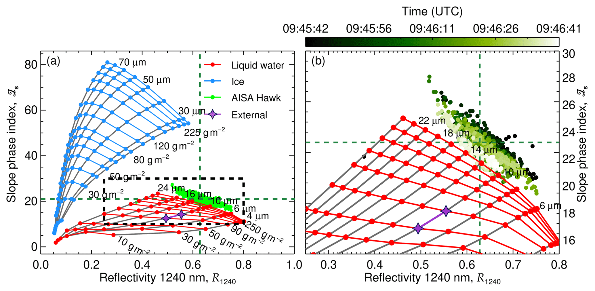
https://www.atmos-chem-phys.net/20/5487/2020/acp-20-5487-2020-f07

Figure 7(a) ℐ_s measured on 2 June 2017 presented as a function of R₁₂₄₀ (green dots). The dashed lines indicate the 25th percentile of R₁₂₄₀ and the 75th percentile of ℐ_s. The two grids represent radiative transfer simulations for a range of pure liquid (red) and pure ice (blue) clouds. The liquid water clouds cover droplets with r_eff between 4 and 24 µm and LWP between 1 and 250 g m⁻². The ice clouds are simulated for columnar ice crystals with r_eff between 28 and 90 µm and IWP between 1 and 250 g m⁻². A SZA of 57.9^∘ was considered. The purple stars show the independent LWP range retrieved by the 89 GHz passive channel of MiRAC and the SID-3 in situ observation of particle size. (b) Zoom into the area highlighted by a dashed rectangle in (a). Color-coded is the acquisition time of measurements illustrating changes along the flight path.

Download

3.2.2 Impact of the vertical distribution of ice and water

Mixed-phase clouds in the Arctic commonly consist of a single layer of supercooled liquid water droplets at cloud top, from which ice crystals precipitate (Mioche et al., 2015), which is in line with the radar/lidar observations presented in Fig. 3. Additionally, Ehrlich et al. (2009) found evidence of ice crystals near the cloud top. Horizontal inhomogeneities in the vertical distribution of the liquid water and ice occur in horizontal scales of 10 m (Korolev and Isaac, 2006; Lawson et al., 2010) and are expected to relate to the small-scale structures (i.e., holes and domes) on the cloud top. Therefore, reproducing the observed trends of R₁₂₄₀ and ℐ_s with simulated mixed-phase clouds can provide information about the horizontal distribution of the cloud thermodynamic phase vertical structure. For this reason, the R₁₂₄₀ and ℐ_s observed on 2 June are compared with three different vertical mixing scenarios. A two-layer cloud scenario with a layer of liquid water droplets at cloud top (750–900 m) and a cloud bottom layer (600–750 m) consisting of precipitating ice particles was assumed to represent the common two-layer vertical thermodynamic phase distribution. In a second and third scenario, a vertically homogeneous mixture of ice and liquid particles was assumed in the cloud layer (600–900 m), to represent the case when both liquid water and ice crystals are also present in the upper cloud top layer. The partitioning between ice and liquid droplets was varied by changing the ice fraction, defined by

\begin{matrix} (7) & IF = \frac{IWP}{TWP} \cdot 100 %, \end{matrix}

with the total water path defined as $TWP = LWP + IWP$ . Pure liquid water clouds correspond to IF=0 % and pure ice clouds to IF=100 %. The slope phase index and the spectral cloud top reflectivity depend on the r_eff of the ice and liquid particles and on the TWP. To inspect the spread of ℐ_s as a function of R₁₂₄₀ for mixed-phase cases with different IF, either the r_eff of the liquid and ice particles or the TWP was kept constant. The approach using a constant value of r_eff was evaluated for the two-layer (Fig. 8a) and the vertically homogeneous mixing scenarios (Fig. 8b), considering a fixed r_eff of 9 µm for the liquid droplets and 50 µm for the ice crystals. The TWP was varied between 25 and 250 g m⁻². The fixed TWP approach was evaluated for the homogeneous mixing scenario (Fig. 8c). Here, the TWP was fixed to 120 g m⁻². In this case, the r_eff ranges between 4 and 24 µm for liquid droplets and between 28 and 90 µm for ice crystals. The three scenarios show grids of ℐ_s where the increasing IF yields different patterns. The comparison with the measurements shows that only the homogeneously mixed scenarios (Fig. 8b and c) may reproduce the measured values of the slope phase index. In the two-layers scenario (Fig. 8a), the liquid water signature dominates ℐ_s, masking the presence of the cloud ice. These mixed-phase clouds need to be formed of at least IF=70 % to cause phase indices that effectively differ from those of pure liquid clouds. Additionally, the TWP required to match the observations exceeds the observed values. This indicates that a significant amount of ice near the cloud top is needed to explain the observed high values of ℐ_s.

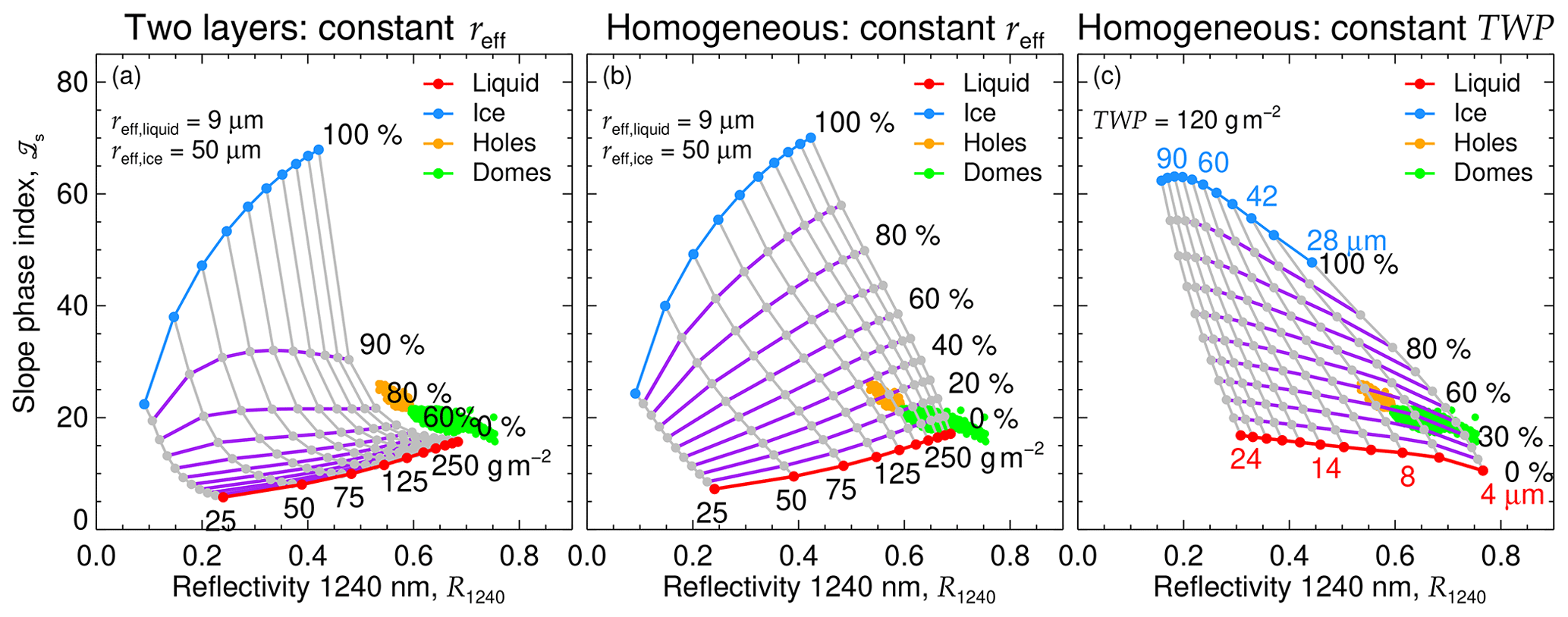
https://www.atmos-chem-phys.net/20/5487/2020/acp-20-5487-2020-f08

Figure 8Comparison of ℐ_s measured on 2 June 2017 as a function of R₁₂₄₀ with three mixing scenarios of mixed-phase clouds. Observations in cloud holes are indicated by orange dots. Green dots represent measurements in cloud domes. Scenario (a) simulates a two-layer cloud, while in scenarios (b) and (c) a homogeneously mixed cloud is assumed. Scenario (b) considers mixed-phase clouds of fixed particle sizes (r_eff,liquid of 9 µm and r_eff,ice of 50 µm) and variable TWP between 25 and 250 g m⁻². The grey solid lines connect clouds of equal TWP and the solid purple lines, clouds of equal IF (indicated by the percentages). In scenario (c), TWP is fixed to 120 g m⁻², and the particle sizes are varied. Here, purple lines connect clouds of equal ice fraction, and the grey lines connect clouds considering equal particle sizes.

Download

The homogeneous phase mixing scenario presented in Fig. 8b could explain part of the observed values of the reflectivity and slope phase index. According to this scenario, the cloud holes (reflectivity below the 25th percentile of R₁₂₄₀) would show higher ice fractions (between 20 % and 40 %) and higher ℐ_s than the cloud dome centers (reflectivity above the 25th percentile of R₁₂₄₀ and phase index below the 75th percentile of ℐ_s), where IF is between 0 % and 20 %. Figure 8c shows the alternative scenario where the TWP is fixed to 120 g m⁻². The simulated clouds cover most of the observed combinations of slope phase indices and reflectivities. In this scenario, the observed cloud would agree with mixed-phase clouds of fixed IF of about 40 %. In contrast to the scenario with fixed r_eff, this pattern indicates that the ice fraction in the cloud centers is similar to that in the cloud holes. The cloud domes centers consist of small droplets with effective radii between 4 and 6 µm and small ice crystals with effective radii between 28 and 36 µm. Larger droplets, with r_eff between 6 and 8 µm, and ice crystals, with r_eff between 36 and 42 µm, are found in the cloud holes. This pattern can be explained by a quick evaporation of small droplets in the cloud holes, leading to a larger r_eff. Both idealized homogeneous mixing scenarios reproduce the observations. However, based on the AISA Hawk measurements of ℐ_s alone, it cannot be judged which scenario is more likely. In reality, neither the particle sizes nor the TWP is horizontally fixed in a cloud field. A combination of both scenarios might be closest to reality. However, due to the large number of possible realizations (combinations of IWP, LWP, r_eff,ice, and r_eff,liquid), it is impossible for it to fully resemble the observations.

4 Comparison of measurements and LES

Comparing simulated cloud top reflectivities and phase index based on ICON-LEM cloud fields with the measurements of AISA Hawk will help to evaluate the conclusions about the vertical structure of the cloud thermodynamic phase drawn in the previous section.

For the two cloud cases of 25 May and 2 June, two regions of 21 km×11 km enclosing the corresponding aircraft measurements were simulated by ICON-LEM (Fig. 2). The resulting cloud profiles are shown in Fig. 9a–c and e–g. The profiles of ice fraction IF(z) shown in Fig. 9b and f are calculated, in correspondence to Eq. (7), by

\begin{matrix} (8) & IF (z) = \frac{IWC (z)}{LWC (z) + IWC (z)} \cdot 100 % . \end{matrix}

On 25 May, the clouds simulated by ICON-LEM are located at higher altitudes than observed. However, the simulated profiles of LWC, IWC, and IF confirm the vertical cloud structure indicated by the active remote sensing measurements (Fig. 3a), with both liquid and ice phases being present. The IWC reaches a maximum value of 0.08 g m⁻³ 430 m below the 0.12 g m⁻³ maximum LWC at 900 m.

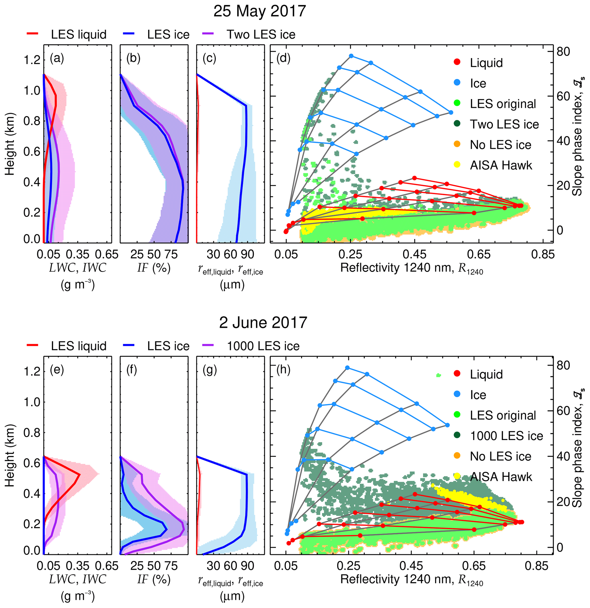
https://www.atmos-chem-phys.net/20/5487/2020/acp-20-5487-2020-f09

Figure 9Mean profiles of liquid and ice water content, ice fraction, and effective radius, with (a), (b), and (c) for 25 May 2017 and (e), (f), and (g) for 2 June 2017, respectively. The shaded areas indicate the standard deviation of the considered distribution. The simulated R₁₂₄₀ and ℐ_s corresponding to the original LES profiles, as well as simulations neglecting the IWC (“No LES ice”) and modifying it (“Two LES ice” for 25 May and “1000 LES ice” for 2 June), are compared with R₁₂₄₀ and ℐ_s of pure-phase clouds and the AISA Hawk measurements in (d) (25 May) and (h) (2 June).

Download

The cloud top reflectivities simulated by libRadtran on the basis of the clouds simulated by ICON-LEM have been used as synthetic measurements to calculate ℐ_s. These synthetic ℐ_s are compared to the observations of AISA Hawk (Figs. 5 and 7). To further test the sensitivity of R₁₂₄₀ and ℐ_s towards the vertical distribution of the cloud thermodynamic phase, additional synthetic cloud top reflectivities (firstly, neglecting the simulated IWC, hence considering pure liquid water clouds, and secondly, doubling the simulated IWC), were also investigated. The comparisons with the AISA Hawk measurements are shown in Fig. 9d. The relation between R₁₂₄₀ and ℐ_s derived from the LES original LWC and IWC profiles shows that the liquid water dominated the cloud top layer, making its R₁₂₄₀ and ℐ_s indiscernible from those of pure liquid water clouds. This is almost identical to the AISA Hawk measurements (Fig. 9d). Only a few data points with higher ℐ_s range above the grid of pure liquid water clouds. These data mostly have low R₁₂₄₀ and can be linked to cloud edges with lower LWP located outside the measurement area of AISA Hawk, where ice fractions are simulated to be higher than observed. Doubling the simulated IWC on 25 May (resulting in a maximum 0.16 g m⁻² at 470 m) yielded a similar result; as for the originally simulated profiles, the R₁₂₄₀ and ℐ_s relation is for most LES pixels dominated by the higher liquid water concentration at cloud top and cannot be differentiated from pure liquid water clouds. However, the enhanced IWC increases ℐ_s beyond values corresponding to pure liquid water clouds for a larger amount of cloud edge pixels than with the IWC originally simulated by ICON-LEM.

On 2 June, ICON-LEM produces a maximum IWC of $1.5 \times 10^{- 4}$ g m⁻³ located 170 m below the maximum 0.37 g m⁻³ LWC at 530 m. As for 25 May, the vertical profiles of IWC and LWC agree with the active remote sensing measurements (Fig. 3b), indicating the presence of both liquid and ice. However, as demonstrated by Fig. 9h, the original IWC simulated by ICON-LEM is too low to effectively impact R₁₂₄₀ and ℐ_s, which follow the pattern of pure liquid water clouds and did not reproduce the AISA Hawk observations. This difference suggests that the ICON-LEM underestimates the concentration of ice for the cloud on 2 June 2017. In a test case, the IWC was increased by a factor of 1000 (maximum value of $1.5 \times 10^{- 4}$ g m⁻³ at 360 m) in the same order of magnitude as the maximum LWC. For this hypothetical cloud field, the radiative transfer simulations reproduced the observed values of ℐ_s, which deviate from the pure liquid case. However, the results of the ICON-LEM simulations show many data points with R₁₂₄₀ way below the observations (R₁₂₄₀<0.45). This indicates that the cloud field produced by the LESs, covering a larger area than the observations, presents significant cloud gaps (low TWP), which were located outside the AISA Hawk measurement region. For the manipulated cloud, these cloud parts show a significant increase in ℐ_s with decreasing R₁₂₄₀, which can be attributed to cloud edges similar to the cold air outbreak case of 25 May.

5 Impact of spatial resolution

The horizontal resolutions of the ICON-LEM (100 m) and the airborne observations (10 m) differ by about 1 order of magnitude. Additionally, satellite-borne imaging spectrometers commonly used to derive global distributions of cloud properties typically do not reach a spatial resolution as high as the AISA Hawk measurements. For instance, the Advanced Very High Resolution Radiometer (AVHRR), the MODerate resolution Imaging Spectroradiometer (MODIS), and the Hyperion imaging spectrometer have resolutions of 1000, 500, and 30 m pixel sizes, respectively (Kaur and Ganju, 2008; Li et al., 2003; Thompson et al., 2018). This raises the question of how much of the observed variability in ℐ_s is lost by horizontal averaging. To assess this question, the AISA Hawk observations of the two cloud cases were averaged for larger pixel sizes. Figures 10 and 11 show a 900 m×900 m subsection of the original fields of R₁₂₄₀ and ℐ_s projected for pixel sizes of 30 m (Hyperion), 90 m (∼ ICON-LEM), 450 m (∼ MODIS), and 900 m (∼ AVHRR). The relationship between ℐ_s and R₁₂₄₀ for the complete fields is illustrated in Fig. 10c, f, i, l, and o for 25 May 2017 and in Fig. 11c, f, i, l, and o for 2 June 2017. The statistics of R₁₂₄₀ and ℐ_s corresponding to the considered pixel sizes for both days are presented in Table 2.

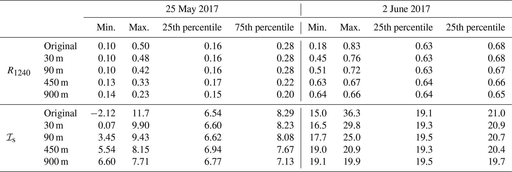
Table 2R₁₂₄₀ and ℐ_s dependence upon the sensor resolution.

Download Print Version | Download XLSX

The smoothing of the cloud scene with increasing pixel size erases the fine spatial structure of the cloud top, which remains only visible for 25 m pixel size. For the cloud case of 25 May 2017, the horizontal averaging mainly impacts the observed cloud geometry. The decreasing contrast between the cloudy and cloud-free pixel changes the cloud mask and eventually causes the loss of the broken cloud nature observed by AISA Hawk. The original range of variability in R₁₂₄₀ between 0.10 and 0.50 decreases to the range between 0.14 and 0.23 at 900 m. The original range of ℐ_s between −2.12 and 11.7 is reduced to the range from 6.60 to 7.71 but always indicates a cloud that is dominated by the liquid layer at cloud top. For the cloud on 2 June 2017 (Fig. 11), the averaging cannot affect the 100 % cloud cover. However, the variability in R₁₂₄₀ becomes significantly reduced for larger pixel sizes (from the original variability of between 0.18 and 0.83 to a variability at 900 m of between 0.64 and 0.66) as no large-scale cloud structures are present. Similarly, the variability in ℐ_s diminishes for observations with coarser spatial resolution from the original range between 15.0 and 36.3 to 19.1 and 19.9 for pixels of 900 m). A coarser resolution removes the contrast between cloud holes, which are typically characterized by the presence of ice crystals (high ℐ_s) and the cloud domes, where liquid droplets dominate (lower ℐ_s). For satellite observations with pixel sizes larger than 90 m, this prevents the characterization and interpretation of the change in cloud phase in the small-scale cloud structure and, therefore, conceals the information about the vertical distribution of the thermodynamic phase contained in the cloud top variability. Highly resolved imaging spectrometer measurements such as the Hyperion and the ICON-LEM, with pixels below 100 m are still able to resolve part of the natural horizontal variability.

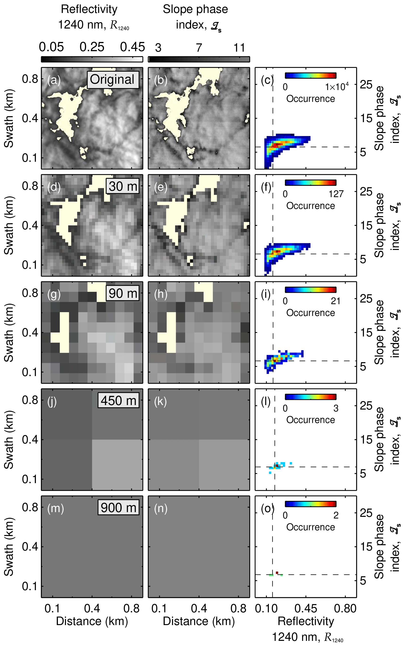
https://www.atmos-chem-phys.net/20/5487/2020/acp-20-5487-2020-f10

Figure 10Slope phase index – 1240 nm reflectivity relationship for five different pixel sizes (original AISA Hawk resolution, 30, 90, 450, and 900 m). Panels (a), (d), and (g) show a 1 km×1 km subsection of R₁₂₄₀ measured on 25 May 2017 as seen by the five different resolutions; (b), (e), and (h) show the corresponding 1 km×1 km ℐ_s; and (c), (f), and (i) present the scatter between both magnitudes for the complete 1 km×4 km field. The dashed lines indicate the 25th percentile of R₁₂₄₀ and ℐ_s for each resolution.

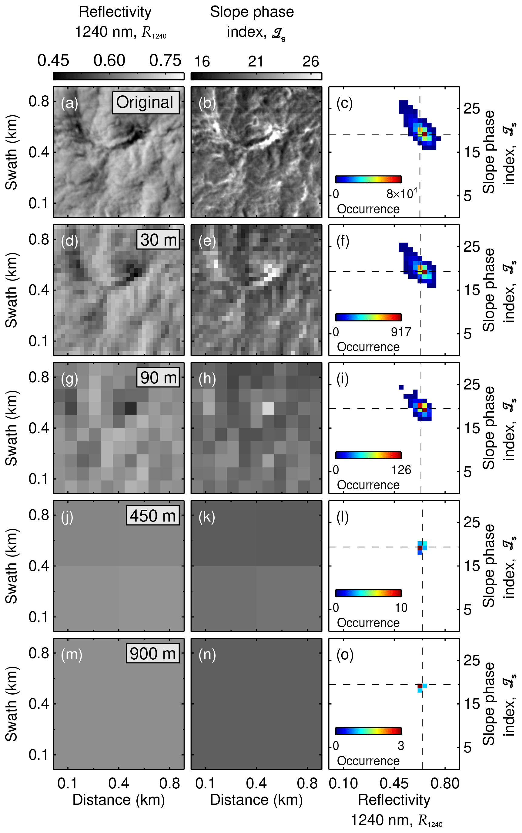
https://www.atmos-chem-phys.net/20/5487/2020/acp-20-5487-2020-f11

Figure 11Slope phase index – 1240 nm reflectivity relationship for five different pixel sizes (original AISA Hawk resolution, 30, 90, 450, and 900 m). Panels (a), (d), and (g) show a 1 km×1 km subsection of R₁₂₄₀ measured on 2 June 2017 as seen by the five different resolutions; (b), (e), and (h), the corresponding 1 km×1 km ℐ_s; and (c), (f), and (i) present the scatter between both magnitudes for the complete 1 km×4 km field. The dashed lines indicate the 25th percentile of R₁₂₄₀ and ℐ_s for each resolution.

6 Conclusions

Based on airborne active and passive remote sensing conducted by a passive imaging spectrometer and vertically resolving instruments, such as lidar and radar, the horizontal and vertical structure of the thermodynamic phase in Arctic mixed-phase cloud cases was characterized for two example clouds observed during a cold air outbreak and a warm air intrusion event. While the spectral imaging was used to identify the structure of the horizontal distribution of the cloud ice at scales down to 10 m, the combined radar and lidar observations revealed the general vertical thermodynamic phase distribution of the clouds.

The two cloud cases were observed over open ocean close to Svalbard (Spitzbergen) during the ACLOUD campaign. The cloud scene sampled on 25 May 2017 evolved within a cold air outbreak, whereas a cloud that had formed in a warm air advection event was sampled on 2 June 2017. For both cloud cases, the combined radar and lidar observations indicated the mixed-phase character of the clouds, with liquid water droplets in the cloud top layer and ice crystals below. While the lidar penetrated the strongly reflecting liquid cloud layer on 25 May, partly until the surface, the strong extinction of the lidar signal close to the cloud top observed on 2 June indicates higher liquid water amounts. The vertical structure of the radar backscatter also differs between both days, with reflectivities reaching the ground on 25 May typical for light snow precipitation. These different cloud vertical structures influenced the ability to detect the ice by the imaging spectrometer observations of AISA Hawk using the slope phase index ℐ_s. On 25 May, ℐ_s is dominated by the liquid water contained at the cloud top layer, which leads to a misclassification as a pure liquid water cloud. The small-scale variability in ℐ_s observed on 25 May relates mostly to the variability in the liquid cloud layers. On 2 June, AISA Hawk measured higher ℐ_s, which hints at the presence of ice crystals in higher cloud layers. Additionally, the LWP, retrieved by assuming pure liquid clouds, shows unrealistically high values compared to the observations by MiRAC, which supports this conclusion. The high values of ℐ_s and the large retrieval bias of LWP are observed close to areas of low cloud reflectivity (cloud holes). The comparison of both cloud cases highlights the limitations of passive remote sensing alone to identify layered mixed-phase structures if the ice is not sufficiently close to the cloud top. In particular in these cases, the combination of active and passive remote sensing is crucial to fully characterize the horizontal and vertical distribution of ice and liquid water particles in mixed-phase clouds.

The highly resolved horizontal distribution of ℐ_s observed on 2 June was analyzed using radiative transfer simulations assuming different mixing scenarios of ice and liquid water content. Two homogeneous mixing scenarios, either keeping the TWP or the particle sizes fixed when changing the ice fraction, did reproduce the observed pattern of variability. However, based on the AISA Hawk measurements of ℐ_s alone, it cannot be judged which scenario is closer to reality. To consider modeled phase-mixing scenarios of IWP, LWP, r_eff,ice, r_eff,liquid, and the vertical cloud structure, the ICON-LEM was applied. The microphysical profiles simulated by ICON-LEM roughly represent major features of the vertical profiles obtained by MiRAC and AMALi for both cloud cases. To compare with the AISA Hawk measurements, radiative transfer simulations of the cloud top were performed on the basis of the ICON-LEM thermodynamic phase profiles. For both cases, the variability in ℐ_s calculated from the simulations is represented by pure liquid water clouds. Enhancing the IWC simulated by ICON-LEM indicates that, whereas on 25 May this behavior is due to the liquid-water-dominated cloud top layer, on 2 June, the simulated concentration of ice crystals is underestimated. In a test case where the IWC was enhanced 1000 times, the simulated cloud central regions showed a comparable structure as observed by AISA Hawk. Additionally, the area simulated by ICON-LEM produced significant cloud gaps not present in the smaller cloud section observed by AISA Hawk. Similarly to 25 May, the cloud gaps present high values of ℐ_s. The comparison of the simulated ℐ_s-R₁₂₄₀ patterns with measured ones can be used to assess the performance of ICON-LEM, which reproduces the vertical structure of the two observed cloud cases but produces too little ice on 2 June. Nevertheless, to fully exploit the measurements–model synergy, synthetic radar and lidar measurements should be simulated based on ICON-LEM, taking into consideration the ice habit observed by in situ measurements as well.

The grid size of ICON-LEM (100 m) is sufficient to resolve the small-scale structure of mixed-phase clouds and to produce different patterns of ℐ_s giving indication of the vertical distribution of the cloud thermodynamic phase. A sensitivity study reducing the horizontal resolution of the passive remote sensing observations illustrated that pixel sizes below 100 m, such as provided by the Hyperion imager spectrometer or airborne spectral imagers, are required to resolve the horizontal distribution of ice and liquid water in Arctic mixed-phase clouds. However, common satellite sensors such as MODIS or AVHRR are not able to capture the small-scale distribution of ℐ_s.

Appendix A: Analysis of 3D effects in the AISA Hawk measurements

The spatially highly resolved radiance fields measured by AISA Hawk are affected by 3D radiative effects caused by the 3D nature of the cloud top. Specifically, (a) horizontal photon transport occurs between neighboring pixels, smoothing the measurements, and (b) cloud top structures cast shadows on the image.

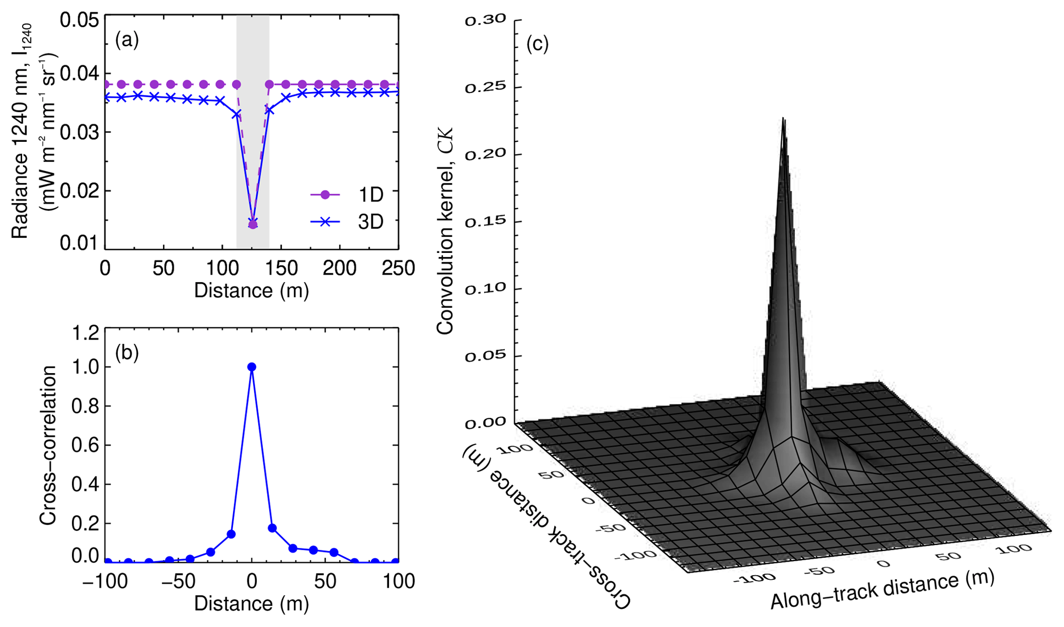
https://www.atmos-chem-phys.net/20/5487/2020/acp-20-5487-2020-f12

Figure A1(a) Comparison of the nadir reflected radiance at 1240 nm by a stratiform cloud deck simulated with 1D and 3D radiative transfer simulations. The cloud contains a 15 m region of pure ice (shaded) embedded between two pure liquid water regions (nonshaded). (b) Cross-correlation between the 1D and the 3D cloud top radiance illustrating the extent of the horizontal photon transport. (c) Normalized convolution kernel based on the cross-correlation of the 1D and 3D simulations and different sun-sensor geometries.

Download

In order to correct the smoothing due to horizontal photon transport, the horizontal sensitivity of each case study was estimated comparing 3D and 1D simulations of the cloud top reflected radiance. The 3D simulations of an idealized cloud field were performed with the Monte Carlo Atmospheric Radiative Transfer Simulator (MCARaTS, Wang et al., 2012), and the 1D simulations were performed with libRadtran. The cloud field considers a liquid water stratiform deck with a LWP similar to the observations (i.e., 30 and 100 g m⁻², respectively), a typical r_eff of 10 µm and solar zenith angle (SZA) of 60 and 57^∘, respectively. A pure ice region of 15 m width, with r_eff of 60 µm and a IWP similar to the LWP, was embedded in the liquid deck. The change in cloud phase in general leads to a reduction of the cloud top radiance in the ice phase area. The 3D and 1D simulations of the 100 g m⁻² case are presented in Fig. A1a. Whereas the 1D simulated radiance stays constant in the liquid water region and decreases sharply within the ice stripe, the horizontal photon transport smooths the transition from the liquid to the ice region in the 3D radiance. The cross-correlation between both simulations, shown in Fig. A1b, provides an estimation of the horizontal displacement of the photons in the 3D simulation, which is effective within distances of about 100 m. The combination of cross-correlation functions calculated for different solar azimuth angles, SAAs, and different sensor viewing angles (therefore accounting for different sun-sensor geometries) yields the 3D normalized convolution kernel CK presented in Fig. A1c. The simulations with LWP of 30 g m⁻² (not shown here) yield a similar result. The derived CK accounts only for the mean photon transport of each field and does not consider local inhomogeneities. Similar to Zinner et al. (2006), in order to avoid overcompensating the horizontal photon transport, the iterative Richardson-Lucy deconvolution algorithm (Richardson, 1972; Lucy, 1974) was applied. After each iteration, the calculated radiance takes the form,

\begin{matrix} (A1) & I_{n + 1} = [(\frac{I}{I_{n} \otimes CK}) \otimes CK], \end{matrix}

where I is the radiance observed by AISA Hawk, I_n is the radiance obtained after the nth iteration, and ⊗ is the convolution operator. Based on the convergence of $| I_{n + 1} - I_{n} | / I_{n}$ , completing four iterations was found to sufficiently increase the sharpness of the measured radiance fields.

However, the second 3D radiative effect, caused by the shadows cast by the cloud top geometry, cannot be easily corrected. Highly spatially resolved measurements of the cloud top geometry would be necessary for correcting self-shading artifacts. Therefore, 3D radiative transfer simulations are used to estimate this 3D radiative effect and analyze whether the observed correlation between R₁₂₄₀, ℐ_s, and LWP are caused by shadows or by inhomogeneous distributions of the cloud thermodynamic phase. Figure A2 presents 3D simulations of two idealized stratiform cloud decks with a constant TWP of 100 g m⁻².

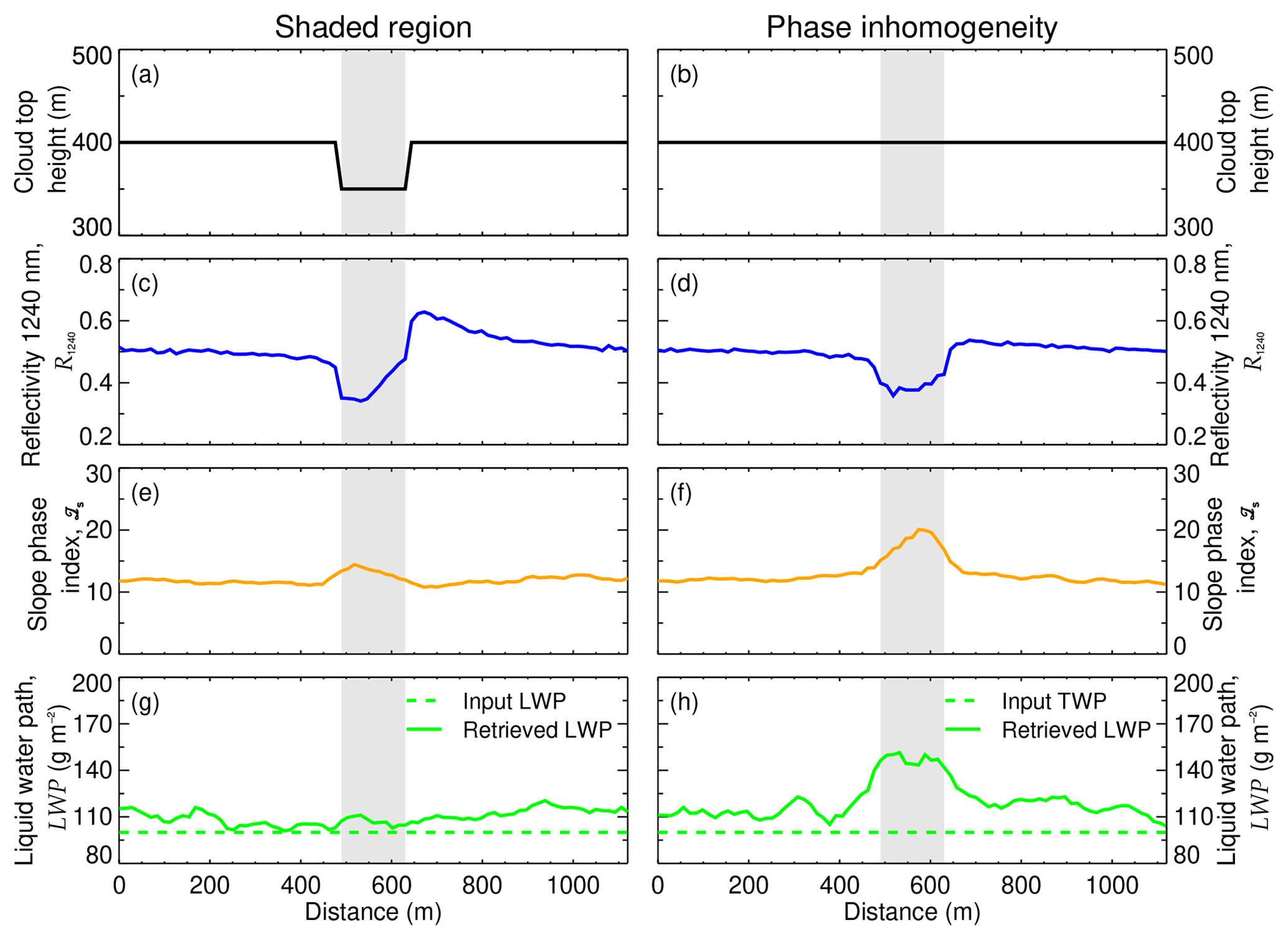
https://www.atmos-chem-phys.net/20/5487/2020/acp-20-5487-2020-f13

Figure A2Cloud top properties of a shaded region (a, c, e, g) compared to a region with a different thermodynamic phase composition (b, d, f, h). The shaded areas indicate the artifact affected areas.

Download

Figure A2a represents a liquid water cloud with an inhomogeneous cloud top height (50 m lower cloud top in the center of the cloud field). For a SZA of 57^∘, similar to the measurement on 2 June, the dip on the cloud top casts a shadow that gets imprinted on R₁₂₄₀ (Fig. A2c), ℐ_s (Fig. A2e), and the retrieved LWP (Fig. A2g). Whereas in the shaded region R₁₂₄₀ decreases on average by 35 % with respect to the nonshaded region, ℐ_s increases on average by 20 %. These opposite effects result in an almost-constant LWP, which does not show a signature of the cloud dip.

Figure A2b shows a pure liquid water cloud with a constant cloud top height and an embedded mixed-phase region of 150 m horizontal extent. The TWP is kept always constant at 100 g m⁻² (i.e., the pure-phase region considers a LWP of 100 g m⁻²; the mixed-phase region considers a LWP of 60 g m⁻² and a IWP of 40 g m⁻²). The liquid water droplets have an r_eff of 10 µm, and the ice crystals have an r_eff of 60 µm. The inhomogeneous phase distribution obviously biases the retrieved cloud top properties and the calculated phase index. In this case, R₁₂₄₀ (Fig. A2d) decreases by 34 % in the mixed-phase region compared to the pure-phase region, and ℐ_s increases by 58 %. However, contrasting the shaded case, the presence of ice crystals leads to a significant increase in LWP by 36 %.

Therefore, the combination of R₁₂₄₀, ℐ_s, and LWP is crucial to interpret the observations of AISA Hawk. Only a simultaneous increase in ℐ_s and LWP when R₁₂₄₀ decreases is indicative of mixed-phase regions. Although we cannot completely discard shading artifacts on the 2 June case study, the observed increment of ℐ_s and LWP in regions of low R₁₂₄₀ agrees with the simulations in Fig. A2d, f, and h and supports the hypothesis of mixed-phase on this day.

Appendix B: LWP retrieval based on passive microwave radiometer measurements

Measurements by the 89 GHz passive channel of the Microwave Radiometer for Arctic Clouds (MiRAC, Mech et al., 2019) were used to estimate the liquid water path (LWP) for the two case studies. Brightness temperatures (TBs) were measured under a tilted angle of 25^∘ with respect to nadir backwards with 1 s integration time. At this frequency, TB depends on the surface emission, dependent in turn on the sea surface temperature (SST) and wind speed, and on atmospheric contributions by atmospheric gases and cloud liquid. Cloud ice does not contribute to the signal, and only strong snowfall could lead to TB reduction by scattering, i.e., 500 g m⁻² snowfall corresponds to about 1–2 K reduction. On short timescales – such as the 2 min long flight tracks – variations are mainly caused by cloud variability. Therefore, a simplified algorithm exploiting the relative change in TB compared to a base state was developed.

For each of the two cases, the closest dropsonde was used to calculate TB as a function of LWP, assuming a cloud between 500 and 100 m above sea level. Within these microwave radiative transfer simulations, the wind speed was taken from the lowest available dropsonde level (5 m s⁻¹ on 25 May and 7.7 m s⁻¹ on 2 June) and the SST (275 K) from climatological data. Liquid water emission leads to an increase in TB above the radiatively cold ocean. When subtracting the clear-sky TB (TB₀), the resulting ΔTB can be well approximated by a third-order regression with an uncertainty of ca. 1 g m⁻² in LWP. Due to the different wind speed and moisture conditions of the two cases, uncertainties of about 5 g m⁻² (12 g m⁻²) at 100 g m⁻² (200 g m⁻²) LWP occur.

The clear-sky TB₀ needs to be derived before applying the simple regression algorithm to calculate ΔTB. For this purpose, we searched for the minimum TB in both cases and checked whether the lidar signal was low. This is to some degree subjective and difficult due to the high cloud presence (see Figs. 4 and 6). In fact, for 2 June a profile approximately 5 min later was chosen. With our best estimates of TB₀ (180 K on 25 May and 186 K on 2 June) for each 1 s measurement, LWP could be derived, yielding a range between 20 and 40 g m⁻² for 25 May and 90 and 120 g m⁻² for 2 June.

While the approach to derive LWP from a single frequency is rather simple, it also presents advantages (for example, absolute calibration errors are avoided due to the use of difference values). Changes in SST, wind speed, and moisture content of the two 1 min time periods are thought to play a minor role and estimated to be below 10 %. The highest uncertainty is thought to stem from the determination of the clear-sky TB₀. However, the maximum uncertainty is estimated to be about 30 g m⁻², and thus, the 2 June case clearly (i) has a higher LWP than the 25 May case and (ii) has a lower LWP than the one estimated by AISA Hawk (Table 1). In the future, additional measurements from higher MiRAC frequency channels and lidar information will be exploited to retrieve a higher accuracy LWP product.

Data availability

The AISA Hawk (Ruiz-Donoso et al., 2019, https://doi.org/10.1594/PANGAEA.902150), SMART (Jäkel et al., 2019, https://doi.org/10.1594/PANGAEA.899177), MiRAC (Kliesch and Mech, 2019, https://doi.org/10.1594/PANGAEA.899565), and AMALi (Neuber et al., 2019, https://doi.org/10.1594/PANGAEA.899962) data, acquired during the ACLOUD campaign, are publicly available on PANGAEA. All other data used and produced in this study are available upon request from the corresponding authors.

Author contributions

MW, AE, and SC designed the experimental basis of this study. ERD, MS, and EJ acquired the measurements of AISA Hawk and SMART. ERD selected the case studies, processed and analyzed the measurements of AISA Hawk, performed the 1D radiative transfer simulations, and drafted the paper. EJ processed the measurements of SMART and performed the 3D radiative transfer simulations. MM and RN acquired the measurements of MiRAC and AMALi. SC, MM, BSK, LLK, and RN processed and analyzed the measurements of MiRAC and AMALi. VS performed the ICON-LEM simulations. AE, MS, and MW provided technical guidance. All authors contributed to the editing of the paper and to the discussion and interpretation of the results.

Competing interests

The authors declare that they have no conflict of interest.

Special issue statement

This article is part of the special issue “Arctic mixed-phase clouds as studied during the ACLOUD/PASCAL campaigns in the framework of (AC)³ (ACP/AMT/ESSD inter-journal SI)”. It is not associated with a conference.

Acknowledgements

We gratefully acknowledge the funding by the Deutsche Forschungsgemeinschaft (DFG, German Research Foundation) – Projektnummer 268020496 – TRR 172, within the Transregional Collaborative Research Center “ArctiC Amplification: Climate Relevant Atmospheric and SurfaCe Processes, and Feedback Mechanisms (AC)³”.

Financial support

This research has been supported by the Deutsche Forschungsgemeinschaft (grant no. 268020496 – TRR 172).

Review statement

This paper was edited by Radovan Krejci and reviewed by David R. Thompson and one anonymous referee.

References

Baum, B., Yang, P., Heymsfield, A. J., Bansemer, A., Cole, B. H., Merrelli, A., Schmitt, C., and Wang, C.: Ice cloud single/scattering property models with the full phase matrix at wavelengths from 0.2 to 100 µm, J. Quant. Spectrosc. Ra., 146, 123–139, https://doi.org/10.1016/j.jqsrt.2014.02.029, 2014. a

Baum, B. A., Heymsfield, A. J., Yang, P., and Bedka, S. T.: Bulk scattering properties for the remote sensing of ice clouds. Part I: Microphysical data and models, J. Appl. Meteorol., 44, 1885–1895, https://doi.org/10.1175/JAM2308.1, 2005. a

Bierwirth, E., Ehrlich, A., Wendisch, M., Gayet, J.-F., Gourbeyre, C., Dupuy, R., Herber, A., Neuber, R., and Lampert, A.: Optical thickness and effective radius of Arctic boundary-layer clouds retrieved from airborne nadir and imaging spectrometry, Atmos. Meas. Tech., 6, 1189–1200, https://doi.org/10.5194/amt-6-1189-2013, 2013. a, b

Chylek, P. and Borel, C.: Mixed phase cloud water/ice structure from high spatial resolution satellite data, Geophys. Res. Lett., 31, L14104, https://doi.org/10.1029/2004GL020428, 2004. a

de Boer, G., Eloranta, E. W., and Shupe, M. D.: Arctic mixed-phase stratiform cloud properties from multiple years of surface-based measurements at two high-latitude locations, J. Atmos. Sci., 66, 2874–2887, https://doi.org/10.1175/2009JAS3029.1, 2009. a

Dipankar, A., Stevens, B., Heinze, R., Moseley, C., Zängl, G., Giorgetta, M., and Brdar, S.: Large eddy simulation using the general circulation model ICON, J. Adv. Model. Earth Sy., 7, 963–986, https://doi.org/10.1002/2015MS000431, 2015. a

Egerer, U., Gottschalk, M., Siebert, H., Ehrlich, A., and Wendisch, M.: The new BELUGA setup for collocated turbulence and radiation measurements using a tethered balloon: first applications in the cloudy Arctic boundary layer, Atmos. Meas. Tech., 12, 4019–4038, https://doi.org/10.5194/amt-12-4019-2019, 2019. a

Ehrlich, A.: The impact of ice crystals on radiative forcing and remote sensing of Arctic boundary-layer mixed-phase clouds, PhD thesis, Johannes Gutenberg University Mainz, Germany, 2009. a

Ehrlich, A., Bierwirth, E., Wendisch, M., Gayet, J.-F., Mioche, G., Lampert, A., and Heintzenberg, J.: Cloud phase identification of Arctic boundary-layer clouds from airborne spectral reflection measurements: test of three approaches, Atmos. Chem. Phys., 8, 7493–7505, https://doi.org/10.5194/acp-8-7493-2008, 2008a. a, b

Ehrlich, A., Wendisch, M., Bierwirth, E., Herber, A., and Schwarzenböck, A.: Ice crystal shape effects on solar radiative properties of Arctic mixed-phase clouds – Dependence on microphysical properties, Atmos. Res., 88, 266–276, 2008b. a

Ehrlich, A., Wendisch, M., Bierwirth, E., Gayet, J.-F., Mioche, G., Lampert, A., and Mayer, B.: Evidence of ice crystals at cloud top of Arctic boundary-layer mixed-phase clouds derived from airborne remote sensing, Atmos. Chem. Phys., 9, 9401–9416, https://doi.org/10.5194/acp-9-9401-2009, 2009. a, b, c

Ehrlich, A., Wendisch, M., Lüpkes, C., Buschmann, M., Bozem, H., Chechin, D., Clemen, H.-C., Dupuy, R., Eppers, O., Hartmann, J., Herber, A., Jäkel, E., Järvinen, E., Jourdan, O., Kästner, U., Kliesch, L.-L., Köllner, F., Mech, M., Mertes, S., Neuber, R., Ruiz-Donoso, E., Schnaiter, M., Schneider, J., Stapf, J., and Zanatta, M.: A comprehensive in situ and remote sensing data set from the Arctic CLoud Observations Using airborne measurements during polar Day (ACLOUD) campaign, Earth Syst. Sci. Data, 11, 1853–1881, https://doi.org/10.5194/essd-11-1853-2019, 2019. a, b, c

Emde, C., Buras-Schnell, R., Kylling, A., Mayer, B., Gasteiger, J., Hamann, U., Kylling, J., Richter, B., Pause, C., Dowling, T., and Bugliaro, L.: The libRadtran software package for radiative transfer calculations (version 2.0.1), Geosci. Model Dev., 9, 1647–1672, https://doi.org/10.5194/gmd-9-1647-2016, 2016. a

Field, P. R., Hogan, R. J., Brown, P. R. A., Illingworth, A. J., Choularton, T. W., Kaye, P. H., Hirst, E., and Greenaway, R.: Simultaneous radar and aircraft observations of mixed-phase cloud at the 100 m scale, Q. J. Roy. Meteor. Soc., 130, 1877–1904, https://doi.org/10.1256/qj.03.102, 2004. a

Fletcher, J., Mason, S., and Jakob, C.: The Climatology, Meteorology, and Boundary Layer Structure of Marine Cold Air Outbreaks in Both Hemispheres, J. Climate, 29, 1999–2014, https://doi.org/10.1175/JCLI-D-15-0268.1, 2016. a, b

Gerber, H., Frick, G., Malinowski, S. P., Brenguier, J.-L., and Burnet, F.: Holes and Entrainment in Stratocumulus, J. Atmos. Sci., 62, 443–459, https://doi.org/10.1175/JAS-3399.1, 2005. a, b

Gerber, H., Frick, G., Malinowski, S. P., Jonsson, H., Khelif, D., and Krueger, S. K.: Entrainment rates and microphysics in POST stratocumulus, J. Geophys. Res.-Atmos., 118, 12,094–12,109, https://doi.org/10.1002/jgrd.50878, 2013. a

Gierens, R., Kneifel, S., Shupe, M. D., Ebell, K., Maturilli, M., and Löhnert, U.: Low-level mixed-phase clouds in a complex Arctic environment, Atmos. Chem. Phys., 20, 3459–3481, https://doi.org/10.5194/acp-20-3459-2020, 2020. a, b

Gregory, D., Morcrette, J.-J., Jakob, C., Beljaars, A. C. M., and Stockdale, T.: Revision of convection, radiation and cloud schemes in the ECMWF integrated forecasting system, Q. J. Roy. Meteor. Soc., 126, 1685–1710, https://doi.org/10.1002/qj.49712656607, 2010. a

Heinze, R., Dipankar, A., Henken, C. C., Moseley, C., Sourdeval, O., Trömel, S., Xie, X., Adamidis, P., Ament, F., Baars, H., Barthlott, C., Behrendt, A., Blahak, U., Bley, S., Brdar, S., Brueck, M., Crewell, S., Deneke, H., Girolamo, P. D., Evaristo, R., Fischer, J., Frank, C., Friederichs, P., Göcke, T., Gorges, K., Hande, L., Hanke, M., Hansen, A., Hege, H., Hoose, C., Jahns, T., Kalthoff, N., Klocke, D., Kneifel, S., Knippertz, P., Kuhn, A., Laar, T. v., Macke, A., Maurer, V., Mayer, B., Meyer, C. I., Muppa, S. K., Neggers, R. A. J., Orlandi, E., Pantillon, F., Pospichal, B., Röber, N., Scheck, L., Seifert, A., Seifert, P., Senf, F., Siligam, P., Simmer, C., Steinke, S., Stevens, B., Wapler, K., Weniger, M., Wulfmeyer, V., Zängl, G., Zhang, D., and Quaas, J.: Large-eddy simulations over Germany using ICON: a comprehensive evaluation, Q. J. Roy. Meteor. Soc., 143, 69–100, https://doi.org/10.1002/qj.2947, 2017. a

Hogan, R. J. and O'Conner, E.: Facilitating cloud radar and lidar algorithms: the Cloudnet Instrument Synergy/Target Categorization Product, Dept. of Meteorol. Univ of Reading, UK, available at: http://www.met.reading.ac.uk/~swrhgnrj/publications/categorization.pdf (last access: 5 March 2020), 2004. a

Horváth, A., Seethala, C., and Deneke, H.: View angle dependence of MODIS liquid water path retrievals in warm oceanic clouds, J. Geophys. Res.-Atmos., 119, 8304–8328, https://doi.org/10.1002/2013JD021355, 2014. a

Jäkel, E., Walter, J., and Wendisch, M.: Thermodynamic phase retrieval of convective clouds: impact of sensor viewing geometry and vertical distribution of cloud properties, Atmos. Meas. Tech., 6, 539–547, https://doi.org/10.5194/amt-6-539-2013, 2013. a

Jäkel, E., Ehrlich, A., Schäfer, M., and Wendisch, M.: Aircraft measurements of spectral solar up- and downward irradiances in the Arctic during the ACLOUD campaign 2017, PANGAEA, https://doi.org/10.1594/PANGAEA.899177, 2019. a

Kalesse, H., de Boer, G., Solomon, A., Oue, M., Ahlgrimm, M., Zhang, D., Shupe, M. D., Luke, E., and Protat, A.: Understanding Rapid Changes in Phase Partitioning between Cloud Liquid and Ice in Stratiform Mixed-Phase Clouds: An Arctic Case Study, Mon. Weather Rev., 144, 4805–4826, https://doi.org/10.1175/MWR-D-16-0155.1, 2016. a

Kaur, R. and Ganju, A.: Cloud classification in NOAA AVHRR imageries using spectral and textural features, J. Ind. Soc. Remote Sens., 36, 167–174, https://doi.org/10.1007/s12524-008-0017-z, 2008. a

Klein, S. A., McCoy, R. B., Morrison, H., Ackerman, A. S., Avramov, A., de Boer, G., Chen, M., Cole, J. N. S., Del Genio, A. D., Falk, M., Foster, M. J., Fridlind, A., Golaz, J.-C., Hashino, T., Harrington, J. Y., Hoose, C., Khairoutdinov, M. F., Larson, V. E., Liu, X., Luo, Y., McFarquhar, G. M., Menon, S., Neggers, R. A. J., Park, S., Poellot, M. R., Schmidt, J. M., Sednev, I., Shipway, B. J., Shupe, M. D., Spangenbery, D. A., Sud, Y. C., Turner, D. D., Veron, D. E., von Salzen, K., Walker, G. K., Wang, Z., Wolf, A. B., Xie, S., Xu, K.-M., Yang, F., and Zhang, G.: Intercomparison of model simulations of mixed-phase clouds observed during the ARM Mixed-Phase Arctic Cloud Experiment. I: Single-layer cloud, Q. J. Roy. Meteor. Soc., 135, 979–1002, https://doi.org/10.1002/qj.416, 2009. a

Kliesch, L.-L. and Mech, M.: Airborne radar reflectivity and brightness temperature measurements with POLAR 5 during ACLOUD in May and June 2017, PANGAEA, https://doi.org/10.1594/PANGAEA.899565, 2019. a

Knudsen, E. M., Heinold, B., Dahlke, S., Bozem, H., Crewell, S., Gorodetskaya, I. V., Heygster, G., Kunkel, D., Maturilli, M., Mech, M., Viceto, C., Rinke, A., Schmithüsen, H., Ehrlich, A., Macke, A., Lüpkes, C., and Wendisch, M.: Meteorological conditions during the ACLOUD/PASCAL field campaign near Svalbard in early summer 2017, Atmos. Chem. Phys., 18, 17995–18022, https://doi.org/10.5194/acp-18-17995-2018, 2018. a

Kokhanovsky, A.: Optical properties of terrestrial clouds, Earth-Sci. Rev., 64, 189–241, https://doi.org/10.1016/S0012-8252(03)00042-4, 2004. a

Kollias, P., Miller, M. A., Luke, E. P., Johnson, K. L., Clothiaux, E. E., Moran, K. P., Widener, K. B., and Albrecht, B. A.: The Atmospheric Radiation Measurement Program Cloud Profiling Radars: Second-Generation Sampling Strategies, Processing, and Cloud Data Products, J. Atmos. Ocean. Tech., 24, 1199–1214, https://doi.org/10.1175/JTECH2033.1, 2007. a

Kolstad, E. W., Bracegirdle, T. J., and Seierstad, I. A.: Marine cold-air outbreaks in the North Atlantic: temporal distribution and associations with large-scale atmospheric circulation, Clim. Dynam., 33, 187–197, 2009. a, b

Korolev, A.: Limitations of the Wegener-Bergeron-Findeisen mechanism in the evolution of mixed-phase clouds, J. Atmos. Sci., 64, 3372–3375, https://doi.org/10.1175/JAS4035.1, 2007. a

Korolev, A. and Field, P. R.: The effect of dynamics on mixed-phase clouds: Theoretical considerations, J. Atmos. Sci., 65, 66–86, https://doi.org/10.1175/2007JAS2355.1, 2008. a

Korolev, A. and Isaac, G. A.: Relative humidity in liquid, mixed-phase, and ice clouds, J. Atmos. Sci., 63, 2865–2880, https://doi.org/10.1175/JAS3784.1, 2006. a, b

Korolev, A., Mcfarquhar, G., R. Field, P., Franklin, C., Lawson, P., Wang, Z., Williams, E., J. Abel, S., Axisa, D., Borrmann, S., Crosier, J., Fugal, J., Krämer, M., Lohmann, U., Schlenczek, O., and Wendisch, M.: Ice Formation and Evolution in Clouds and Precipitation: Measurement and Modeling Challenges. Chapter 5: Mixed-phase clouds: progress and challenges., AMS Meteorological Monographs, pp. 5.1–5.50, 2017. a

Kostka, P. M., Weissmann, M., Buras, R., Mayer, B., and Stiller, O.: Observation Operator for Visible and Near-Infrared Satellite Reflectances, J. Atmos. Ocean. Tech., 31, 1216–1233, https://doi.org/10.1175/JTECH-D-13-00116.1, 2014. a

Langenbach, A., Baumgarten, G., Fiedler, J., Lübken, F.-J., von Savigny, C., and Zalach, J.: Year-round stratospheric aerosol backscatter ratios calculated from lidar measurements above northern Norway, Atmos. Meas. Tech., 12, 4065–4076, https://doi.org/10.5194/amt-12-4065-2019, 2019. a

Lawson, R. P., Jensen, E., Mitchell, D. L., Baker, B., Mo, Q. X., and Pilson, B.: Microphysical and radiative properties of tropical clouds investigated in TC4 and NAMMA, J. Geophys. Res., 115, D00J08, https://doi.org/10.1029/2009JD013017, 2010. a, b

Li, J., Menzel, W. P., Yang, Z., Frey, R. A., and Ackerman, S. A.: High-Spatial-Resolution Surface and Cloud-Type Classification from MODIS Multispectral Band Measurements, J. Appl. Meteorol., 42, 204–226, https://doi.org/10.1175/1520-0450(2003)042<0204:HSRSAC>2.0.CO;2, 2003. a

Lindsay, R., Wensnahan, M., Schweiger, A., and Zhang, J.: Evaluation of Seven Different Atmospheric Reanalysis Products in the Arctic, J. Climate, 27, 2588–2606, https://doi.org/10.1175/JCLI-D-13-00014.1, 2014. a

Loewe, K., Ekman, A. M. L., Paukert, M., Sedlar, J., Tjernström, M., and Hoose, C.: Modelling micro- and macrophysical contributors to the dissipation of an Arctic mixed-phase cloud during the Arctic Summer Cloud Ocean Study (ASCOS), Atmos. Chem. Phys., 17, 6693–6704, https://doi.org/10.5194/acp-17-6693-2017, 2017. a

Lucy, L. B.: An iterative technique for the rectification of observed distributions, Astron. J., 79, 745, https://doi.org/10.1086/111605, 1974. a

Luo, Y. L., Xu, K. M., Morrison, H., McFarquhar, G. M., Wang, Z., and Zhang, G.: Multi-layer arctic mixed-phase clouds simulated by a cloud-resolving model: Comparison with ARM observations and sensitivity experiments, J. Geophys. Res., 113, D12208, https://doi.org/10.1029/2007JD009563, 2008. a

Maahn, M., Löhnert, U., Kollias, P., Jackson, R. C., and McFarquhar, G. M.: Developing and Evaluating Ice Cloud Parameterizations for Forward Modeling of Radar Moments Using in situ Aircraft Observations, J. Atmos. Ocean. Tech., 32, 880–903, https://doi.org/10.1175/JTECH-D-14-00112.1, 2015. a

Marchand, R. T., Ackermann, T. P., and Moroney, C.: An assessment of Multiangle Imaging Spectroradiometer (MISR) stereoderived cloud top heights and cloud top winds using groundbased radar, lidar, and microwave radiometers, J. Geophys. Res., 112, D06204, https://doi.org/10.1029/2006JD007091, 2007. a

Marshak, A., Platnick, S., Varnai, T., Wen, G. Y., and Cahalan, R. F.: Impact of three-dimensional radiative effects on satellite retrievals of cloud droplet sizes, J. Geophys. Res., 111, D09207, https://doi.org/10.1029/2005JD006686, 2006. a

Martin, G. M., Johnson, D. W., and Spice, A.: The measurement and parameterization of effective radius of droplets in warm stratocumulus, J. Atmos. Sci., 51, 1823–1842, https://doi.org/10.1175/1520-0469(1994)051<1823:TMAPOE>2.0.CO;2, 1994. a

Mayer, B. and Kylling, A.: Technical note: The libRadtran software package for radiative transfer calculations – description and examples of use, Atmos. Chem. Phys., 5, 1855–1877, https://doi.org/10.5194/acp-5-1855-2005, 2005. a

McFarquhar, G. M., Zhang, G., Poellot, M. R., Kok, G. L., Mccoy, R., Tooman, T., Fridlind, A., and Heymsfield, A. J.: Ice properties of single-layer stratocumulus during the Mixed-Phase Arctic Cloud Experiment: 1. Observations, J. Geophys. Res., 112, D24201, https://doi.org/10.1029/2007JD008633, 2007. a, b

McGill, M. J., Li, L., Hart, W. D., Heymsfield, G. M., Hlavka, D. L., Racette, P. E., Tian, L., Vaughan, M. A., and Winker, D. M.: Combined lidar-radar remote sensing: Initial results from CRYSTAL-FACE, J. Geophys. Res., 109, D07203, https://doi.org/10.1029/2003JD004030, 2004. a

Mech, M., Kliesch, L.-L., Anhäuser, A., Rose, T., Kollias, P., and Crewell, S.: Microwave Radar/radiometer for Arctic Clouds (MiRAC): first insights from the ACLOUD campaign, Atmos. Meas. Tech., 12, 5019–5037, https://doi.org/10.5194/amt-12-5019-2019, 2019. a, b, c

Mellado, J. P.: Cloud-Top Entrainment in Stratocumulus Clouds, Annu. Rev. Fluid Mech., 49, 145–69, https://doi.org/10.1146/annurev-fluid-010816-060231, 2017. a

Miller, S. D., Noh, Y.-J., and Heidinger, A. K.: Liquid-top mixed-phase cloud detection from shortwave-infrared satellite radiometer observations: A physical basis, J. Geophys. Res., 119, 8245–8267, https://doi.org/10.1002/2013JD021262, 2014. a

Mioche, G., Jourdan, O., Ceccaldi, M., and Delanoë, J.: Variability of mixed-phase clouds in the Arctic with a focus on the Svalbard region: a study based on spaceborne active remote sensing, Atmos. Chem. Phys., 15, 2445–2461, https://doi.org/10.5194/acp-15-2445-2015, 2015. a, b, c

Mioche, G., Jourdan, O., Delanoë, J., Gourbeyre, C., Febvre, G., Dupuy, R., Monier, M., Szczap, F., Schwarzenboeck, A., and Gayet, J.-F.: Vertical distribution of microphysical properties of Arctic springtime low-level mixed-phase clouds over the Greenland and Norwegian seas, Atmos. Chem. Phys., 17, 12845–12869, https://doi.org/10.5194/acp-17-12845-2017, 2017. a, b, c, d

Morrison, H., de Boer, G., Feingold, G., Harrington, J., Shupe, M. D., and Sulia, K.: Resilience of persistent Arctic mixed-phase clouds, Nat. Geosci., 5, 11–17, https://doi.org/10.1038/NGEO1332, 2012. a, b, c

Nakajima, T. and King, M.: Determination of the optical thickness and effective particle radius of clouds from reflected solar radiation measurements. Part I: Theory, J. Atmos. Sci., 47, 1878–1893, https://doi.org/10.1175/1520-0469(1990)047<1878:DOTOTA>2.0.CO;2, 1990. a

Neggers, R. A. J., Chylik, J., Egerer, U., Griesche, H., Schemann, V., Seifert, P., Siebert, H., and Macke, A.: Local and Remote Controls on Arctic Mixed-Layer Evolution, J. Adv. Model. Earth Sy., 11, 2214–2237, https://doi.org/10.1029/2019MS001671, 2019. a

Neuber, R., Schmidt, L. V., Ritter, C., and Mech, M.: Cloud top altitudes observed with airborne lidar during the ACLOUD campaign, PANGAEA, https://doi.org/10.1594/PANGAEA.899962, 2019. a

Nomokonova, T., Ebell, K., Löhnert, U., Maturilli, M., Ritter, C., and O'Connor, E.: Statistics on clouds and their relation to thermodynamic conditions at Ny-Ålesund using ground-based sensor synergy, Atmos. Chem. Phys., 19, 4105–4126, https://doi.org/10.5194/acp-19-4105-2019, 2019. a, b

Pilewskie, P. and Twomey, S.: Discrimination of ice from water in clouds by optical remote sensing, Atmos. Res., 21, 113–122, https://doi.org/10.1016/0169-8095(87)90002-0, 1987. a

Pithan, F., Svensson, G., Caballero, R., Chechin, D., Cronin, T. W., Ekman, A. M. L., Neggers, R., Shupe, M. D., Solomon, A., Tjernström, M., and Wendisch, M.: Role of air-mass transformations in exchange between the Arctic and mid-latitudes, Nat. Geosci., 11, 805–812, https://doi.org/10.1038/s41561-018-0234-1, 2018. a, b, c

Platnick, S.: Vertical photon transport in cloud remote sensing problems, J. Geophys. Res., 105, 22919–22935, https://doi.org/10.1029/2000JD900333, 2000. a, b

Pu, R.: Hyperspectral remote sensing: Fundamentals and practices, https://doi.org/10.1201/9781315120607, 2017. a

Richardson, W. H.: Bayesian-Based Iterative Method of Image Restoration, J. Opt. Soc. Am., 62, 55–59, https://doi.org/10.1364/JOSA.62.000055, 1972. a

Riedi, J., Marchant, B., Platnick, S., Baum, B. A., Thieuleux, F., Oudard, C., Parol, F., Nicolas, J.-M., and Dubuisson, P.: Cloud thermodynamic phase inferred from merged POLDER and MODIS data, Atmos. Chem. Phys., 10, 11851–11865, https://doi.org/10.5194/acp-10-11851-2010, 2010. a

Roesler, E. L., Posselt, D. J., and Rood, R. B.: Using large eddy simulations to reveal the size, strength, and phase of updraft and downdraft cores of an Arctic mixed-phase stratocumulus cloud, J. Geophys. Res.-Atmos., 122, 4378–4400, https://doi.org/10.1002/2016JD026055, 2017. a, b

Ruiz-Donoso, E., Ehrlich, A., Schäfer, M., Jäkel, E., and Wendisch, M.: Spectral solar cloud top radiance measured by airborne spectral imaging during the ACLOUD campaign in 2017, PANGAEA, https://doi.org/10.1594/PANGAEA.902150, 2019. a

Schäfer, M., Bierwirth, E., Ehrlich, A., Heyner, F., and Wendisch, M.: Retrieval of cirrus optical thickness and assessment of ice crystal shape from ground-based imaging spectrometry, Atmos. Meas. Tech., 6, 1855–1868, https://doi.org/10.5194/amt-6-1855-2013, 2013. a, b, c

Schäfer, M., Bierwirth, E., Ehrlich, A., Jäkel, E., Werner, F., and Wendisch, M.: Directional, horizontal inhomogeneities of cloud optical thickness fields retrieved from ground-based and airbornespectral imaging, Atmos. Chem. Phys., 17, 2359–2372, https://doi.org/10.5194/acp-17-2359-2017, 2017. a

Schäfer, M., Loewe, K., Ehrlich, A., Hoose, C., and Wendisch, M.: Simulated and observed horizontal inhomogeneities of optical thickness of Arctic stratus, Atmos. Chem. Phys., 18, 13115–13133, https://doi.org/10.5194/acp-18-13115-2018, 2018. a, b

Schemann, V. and Ebell, K.: Simulation of mixed-phase clouds with the ICON large-eddy model in the complex Arctic environment around Ny-Ålesund, Atmos. Chem. Phys., 20, 475–485, https://doi.org/10.5194/acp-20-475-2020, 2020. a

Schnaiter, M. and Järvinen, E.: SID-3 1Hz size distribution of cloud particles during the ACLOUD campaign in 2017, PANGAEA, https://doi.org/10.1594/PANGAEA.900261, 2019. a

Sedlar, J. and Tjernström, M.: Clouds, warm air, and a climate cooling signal over the summer Arctic, Geophys. Res. Lett., 44, 1095–1103, https://doi.org/10.1002/2016GL071959, 2017. a, b, c

Seifert, A. and Beheng, K. D.: A two-moment cloud microphysics parameterization for mixed-phase clouds. Part 1: Model description, Meteorol. Atmos. Phys., 92, 45–66, https://doi.org/10.1007/s00703-005-0112-4, 2006. a, b

Serreze, M. C. and Barry, R. G.: Processes and impacts of Arctic amplification: A research synthesis, Global Planet. Change, 77, 85–96, https://doi.org/10.1016/j.gloplacha.2011.03.004, 2011. a

Shettle, E.: Models of aerosols, clouds, and precipitation for atmospheric propagation studies, AGARD Conf. Proce., 1, 1990. a

Shupe, M. D.: A ground-based multisensor cloud phase classifier, Geophys. Res. Lett., 34, L22809, https://doi.org/10.1029/2007GL031008, 2007. a

Shupe, M. D.: Clouds at Arctic atmospheric observatories. Part II: Thermodynamic phase characteristics, J. Appl. Meteorol. Clim., 50, 645–661, https://doi.org/10.1175/2010JAMC2468.1, 2011. a, b

Shupe, M. D., Uttal, T., and Matrosov, S. Y.: Arctic cloud microphysics retrievals from surface-based remote sensors at SHEBA, J. Appl. Meteor., 44, 1544–1562, https://doi.org/10.1175/JAM2297.1, 2005. a

Shupe, M. D., Matrosov, S. Y., and Uttal, T.: Arctic mixed-phase cloud properties derived from surface-based sensors at SHEBA, J. Atmos. Sci., 63, 697–711, https://doi.org/10.1175/JAS3659.1, 2006. a, b, c, d

Shupe, M. D., Kollias, P., Persson, P. O. G., and McFarquhar, G. M.: Vertical motions in Arctic mixed-phase stratiform clouds, J. Atmos. Sci., 65, 1304–1322, https://doi.org/10.1175/2007JAS2479.1, 2008. a, b

Stachlewska, I. S., Neuber, R., Lampert, A., Ritter, C., and Wehrle, G.: AMALi – the Airborne Mobile Aerosol Lidar for Arctic research, Atmos. Chem. Phys., 10, 2947–2963, https://doi.org/10.5194/acp-10-2947-2010, 2010. a, b

Stamnes, K., Tsay, S.-C., Wiscombe, W., and Laszlo, I.: DISORT, a General-Purpose Fortran Program for Discrete-Ordinate-Method Radiative Transfer in Scattering and Emitting Layered Media: Documentation of Methodology, Tech. rep., Dept. of Physics and Engineering Physics, Stevens Institute of Technology, Hoboken, NJ 07030, 2000. a

Stephens, G., Vane, D., Boain, R., Mace, G., Sassen, K., Wang, Z., Illingworth, A., O'Connor, E., Rossow, W., Durden, S., Miller, S., Austin, R., Benedetti, A., Mitrescu, C., and the CloudSat Science Team: The CloudSat mission and the A-train, B. Am. Meteorol. Soc., 83, 1771–1790, https://doi.org/10.1175/BAMS-83-12-1771, 2002. a

Tan, I. and Storelvmo, T.: Sensitivity Study on the Influence of Cloud Microphysical Parameters on Mixed-Phase Cloud Thermodynamic Phase Partitioning in CAM5, J. Atmos. Sci., 73, 709–728, https://doi.org/10.1175/JAS-D-15-0152.1, 2016. a

Tan, I. and Storelvmo, T.: Evidence of Strong Contributions From Mixed-Phase Clouds to Arctic Climate Change, Geophys. Res. Lett., 46, 2894–2902, https://doi.org/10.1029/2018GL081871, 2019. a

Thompson, D. R., McCubbin, I., Gao, B. C., Green, R. O., Matthews, A. A., Mei, F., Meyer, K. G., Platnick, S., Schmid, B., Tomlinson, J., and Wilcox, E.: Measuring cloud thermodynamic phase with shortwave infrared imaging spectroscopy, J. Geophys. Res.-Atmos., 121, 9174–9190, https://doi.org/10.1002/2016JD024999, 2016. a, b

Thompson, D. R., Kahn, B. H., Green, R. O., Chien, S. A., Middleton, E. M., and Tran, D. Q.: Global spectroscopic survey of cloud thermodynamic phase at high spatial resolution, 2005–2015, Atmos. Meas. Tech., 11, 1019–1030, https://doi.org/10.5194/amt-11-1019-2018, 2018. a

Tjernström, M., Shupe, M. D., Brooks, I. M., Persson, P. O. G., Prytherch, J., Salisbury, D. J., Sedlar, J., Achtert, P., Brooks, B. J., Johnston, P. E., Sotiropoulou, G., and Wolfe, D.: Warm-air advection, air mass transformation and fog causes rapid ice melt, Geophys. Res. Lett., 42, 5594–5602, https://doi.org/10.1002/2015GL064373, 2015. a

Vochezer, P., Järvinen, E., Wagner, R., Kupiszewski, P., Leisner, T., and Schnaiter, M.: In situ characterization of mixed phase clouds using the Small Ice Detector and the Particle Phase Discriminator, Atmos. Meas. Tech., 9, 159–177, https://doi.org/10.5194/amt-9-159-2016, 2016. a

Wang, S., Zheng, X., and Jiang, Q.: Strongly sheared stratocumulus convection: an observationally based large-eddy simulation study, Atmos. Chem. Phys., 12, 5223–5235, https://doi.org/10.5194/acp-12-5223-2012, 2012. a

Wendisch, M., Müller, D., Schell, D., and Heintzenberg, J.: An airborne spectral albedometer with active horizontal stabilization, J. Atmos. Ocean. Tech., 18, 1856–1866, https://doi.org/10.1175/1520-0426(2001)018<1856:AASAWA>2.0.CO;2, 2001. a

Wendisch, M., Brückner, M., Burrows, J. P., Crewell, S., Dethloff, K., Ebell, K., Lüpkes, C., Macke, A., Notholt, J., Quaas, J., Rinke, A., and Tegen, I.: Understanding causes and effects of rapid warming in the Arctic, Eos, 98, 22–26, https://doi.org/10.1029/2017EO064803, 2017. a

Wendisch, M., Macke, A., Ehrlich, A., Lüpkes, C., Mech, M., Chechin, D., Dethloff, K., Velasco, C. B., Bozem, H., Brückner, M., Clemen, H.-C., Crewell, S., Donth, T., Dupuy, R., Ebell, K., Egerer, U., Engelmann, R., Engler, C., Eppers, O., Gehrmann, M., Gong, X., Gottschalk, M., Gourbeyre, C., Griesche, H., Hartmann, J., Hartmann, M., Heinold, B., Herber, A., Herrmann, H., Heygster, G., Hoor, P., Jafariserajehlou, S., Jäkel, E., Järvinen, E., Jourdan, O., Kästner, U., Kecorius, S., Knudsen, E. M., Köllner, F., Kretzschmar, J., Lelli, L., Leroy, D., Maturilli, M., Mei, L., Mertes, S., Mioche, G., Neuber, R., Nicolaus, M., Nomokonova, T., Notholt, J., Palm, M., van Pinxteren, M., Quaas, J., Richter, P., Ruiz-Donoso, E., Schäfer, M., Schmieder, K., Schnaiter, M., Schneider, J., Schwarzenböck, A., Seifert, P., Shupe, M. D., Siebert, H., Spreen, G., Stapf, J., Stratmann, F., Vogl, T., Welti, A., Wex, H., Wiedensohler, A., Zanatta, M., and Zeppenfeld, S.: The Arctic Cloud Puzzle: Using ACLOUD/PASCAL Multiplatform Observations to Unravel the Role of Clouds and Aerosol Particles in Arctic Amplification, B. Am. Meteorol. Soc., 100, 841–871, https://doi.org/10.1175/BAMS-D-18-0072.1, 2019. a, b

Werner, F., Siebert, H., Pilewskie, P., Schmeissner, T., Shaw, R. A., and Wendisch, M.: New airborne retrieval approach for trade wind cumulus properties under overlying cirrus, J. Geophys. Res.-Atmos., 118, 3634–3649, https://doi.org/10.1002/jgrd.50334, 2013. a

Werner, F., Ditas, F., Siebert, H., Simmel, M., Wehner, B., Pilewskie, P., Schmeissner, T., Shaw, R. A., Hartmann, S., Wex, H., Roberts, G. C., and Wendisch, M.: Twomey effect observed from collocated microphysical and remote sensing measurements over shallow cumulus, J. Geophys. Res., 119, 1534–1545, https://doi.org/10.1002/2013JD020131, 2014. a

Wesche, C., Steinhage, D., and Nixdorf, U.: Polar aircraft Polar5 and Polar6 operated by the Alfred Wegener Institute, J. Large-Scale Res. Facilities, 2, A87, https://doi.org/10.17815/jlsrf-2-153, 2016. a

Woods, C., Caballero, R., and Svensson, G.: Large-scale circulation associated with moisture intrusions into the Arctic during winter, Geophys. Res. Lett., 40, 4717–4721, https://doi.org/10.1002/grl.50912, 2013. a, b

Yang, P., Liou, K. N., Wyser, K., and Mitchell, D.: Parameterization of the scattering and absorption properties of individual ice crystals, J. Geophys. Res., 105, 4.699–4.718, https://doi.org/10.1029/1999JD900755, 2000. a

Zhou, L., Liu, Q., Liu, D., Xie, L., Qi, L., and Liu, X.: Validation of MODIS liquid water path for oceanic nonraining warm clouds: Implications on the vertical profile of cloud water content, J. Geophys. Res.-Atmos., 121, 4855–4876, https://doi.org/10.1002/2015JD024499, 2016. a

Zinner, T. and Mayer, B.: Remote sensing of stratocumulus clouds: Uncertainties and biases due to inhomogeneity, J. Geophys. Res.-Atmos., 111, D14209, https://doi.org/10.1029/2005JD006955, 2006. a

Zinner, T., Mayer, B., and Schröder, M.: Determination of 3D cloud structures from high resolution radiance data, J. Geophys. Res., 111, D08204, https://doi.org/10.1029/2005JD006062, 2006. a