The SHOW instrument is a spatial heterodyne spectrometer (SHS) that has been optimized for limb-viewing observations of limb-scattered sunlight within a vibrational band of water. The limb is imaged conjugate to the SHS interference fringes such that each interferogram row and subsequently each spectral row in the image are mapped 1-to-1 to the line of sight at the limb. Each sample provides a vertically resolved spectral image with ∼0.03 nm spectral resolution in a 3 nm window centered on 1364.5 nm. These vertically resolved spectral images are inverted using a non-linear optimal estimation approach to obtain the vertical distribution of water vapour. The SHOW measurement technique and retrieval algorithm are discussed in previous publications (Langille et al., 2017, 2018, 2019).

Table 1SHOW ER-2 instrument parameters.

Download Print Version | Download XLSX

The prototype SHOW instrument is optimized for observations from NASA's ER-2 airplane and is mounted in a forward-looking wing pod to observe a 4^∘ × 5.1^∘ (vertical × horizontal) field of view. Flying at an altitude of 21 km, the viewing geometry and optical configuration provide a vertical sampling at the limb tangent point of 51 to 171 m, increasing towards the ground tangent. The instrument utilizes anamorphic optics to average over the scene in the horizontal dimension; therefore, no horizontal (longitudinal) scene information is obtained. Using this configuration, retrievals are performed on a 250 m retrieval grid with no smoothing to provide an approximate vertical resolution of 250 m from 13 km up to 18 km with precisions better than 1 ppm. The instrument can be operated using sampling rates from the 0.1 Hz up to the 2 Hz mode; however, the measurements discussed in this paper are obtained using a sampling rate of 1 Hz. This provides an approximate raw along-track sampling of ∼0.5 km at the surface. The primary instrument specifications are listed in Table 1, and the full instrument configuration is presented in Langille et al. (2019).

The measurements discussed in this paper were obtained during a flight aboard the ER-2 performed on 21 July 2017 between 18:00 and 19:00 UTC off the western coast of North America. For analysis of the meteorological fields within this measurement window, we utilize the ECMWF (ERA5) reanalysis products, which are provided in 1 h time steps on a 0.25^∘ × 0.25^∘ grid (latitude × longitude) at 37 pressure levels from 1 hPa up to 1000 hPa.

To provide the dynamical background of the flight track, the zonal wind at the 175 hPa level (approximately 13 km altitude) for the 18:00:00 UTC time step on 21 July 2017 is shown in Fig. 1. The zonal wind field shows a double-jet structure, with the subtropical jet located near 35^∘ N and the polar jet near 45^∘ N. Both features have jet cores (with winds > 40 m s⁻¹) that are located over the Pacific Ocean. As the subtropical jet shifts north, downstream in an anticyclonic flow, the two jets merge over North America. This configuration is formed with a large-scale Rossby wave-breaking event that developed over several days prior to the SHOW measurements and is demonstrated in Fig. 2 using the 380 K isentropic potential vorticity in 48 h intervals over a 6 d period. To further connect with the ER-2 track, the potential vorticity on the 380 and 400 K surfaces is shown in Fig. 3 for the 21 July 2017 time step. Here, we used 6 PVU to identify the separation between tropospheric air on the 380 K surface (Kunz et al., 2011a, b), which is noted by the white transition region between red (low-PV air and tropospheric) and blue (high-PV air and stratospheric) colours in the figure. A well-defined low-PV structure consistent with tropospheric air is observed on the 380 K surface that extends from the western Pacific up to the extratropical region over North America as a result of the wave breaking. Similarly, we used 8 PVU to represent this separation on the 400 K isentropic surface, which consistently highlighted the filament of tropical air (more tropospheric) in the background of extratropical (lower stratospheric) background.

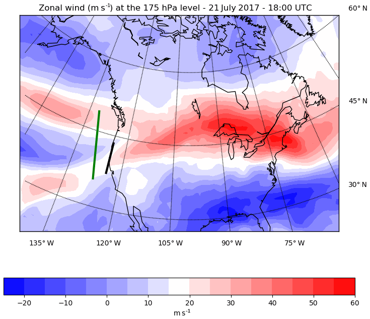
Figure 1Zonal wind on the 175 hPa surface for the 18:00 UTC, 21 July 2017, time step. The ER-2 flight track with the SHOW measurements is shown as the black line, and the closest measurement track of the AURA–MLS instrument is shown as the dark green line.

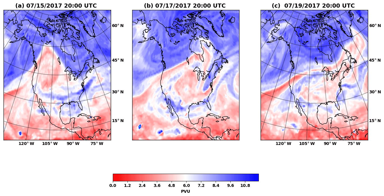
Figure 2Potential vorticity on the 380 K isentropic surface on 15, 17, and 19 July 2017 at 20:00 UTC, showing a Rossby wave-breaking event several days prior to the SHOW measurements.

To characterize the dynamical structure vertically, the height of the thermal tropopause and the occurrence of the double tropopause are shown in Fig. 4. Here the tropopause is derived using the ERA5 temperature field using the lapse rate definition (WMO, 1957, 1992) with a modification. The modified version locates the first tropopause as the lowest level where the lapse rate drops below 2 K km⁻¹ and remains below that value on average for 1 km (instead of 2 km). A second tropopause is identified if the lapse rate increases above 2 K km⁻¹ (instead of 3 K km⁻¹) and then decreases again below 2 K km⁻¹. This is done to remedy the coarse vertical resolution of the of the temperature data. This type of modification has been recognized to allow identification of the double tropopause derived from coarse-resolution temperature data that are more consistent with high-resolution observational data (Randel et al., 2007). Our goal here is to highlight the spatial extent of the layered static stability structure as discussed in Sects. 4–5. The height distribution of the primary tropopause is shown in Fig. 4a. The distribution of the secondary tropopause, shown in Fig. 4b, is consistent with the formation mechanism of a poleward wave breaking along the subtropical jet (Pan et al., 2009). Although not shown here, the double-tropopause features have varying strength from time step to time step on the days leading up to and after the flight. Occurrences of double tropopauses are common in this region, with the highest occurrence rate in the winter (Swartz et al., 2015); however, they are also observed in the summer season (Añel et al., 2008).

The ER-2 flight track with the SHOW instrument for the 18:00 to 19:00 UTC time period, as indicated in Figs. 1, 3, and 4, includes the edge of a large double-tropopause region that extends off the West Coast of the United States. For process verification using an independent measurement, we identified a near co-located MLS satellite observation track, also marked in Figs. 1, 3, and 4. Analyses of the SHOW and MLS measurements are discussed in Sects. 4 and 5 respectively.

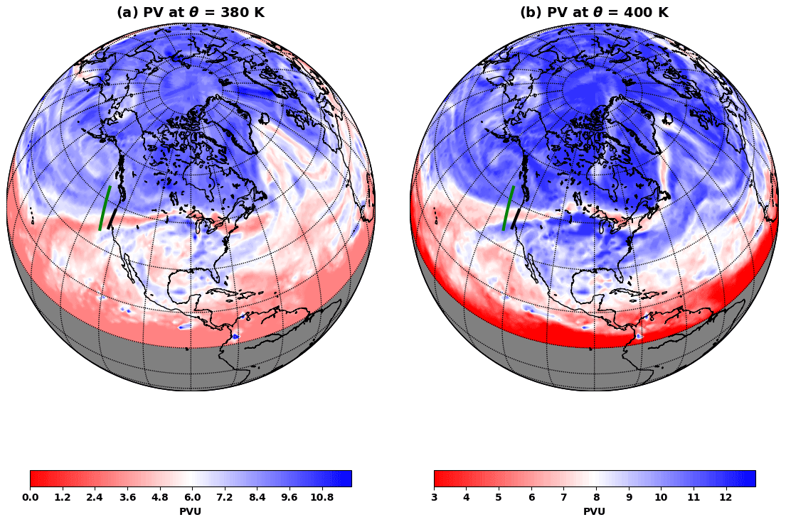
Figure 3Potential vorticity on the 380 (a) and 400 K (b) isentropic surfaces for the 18:00 UTC, 21 July 2017, time step. The measurement tracks of SHOW and MLS are shown in black and green respectively.

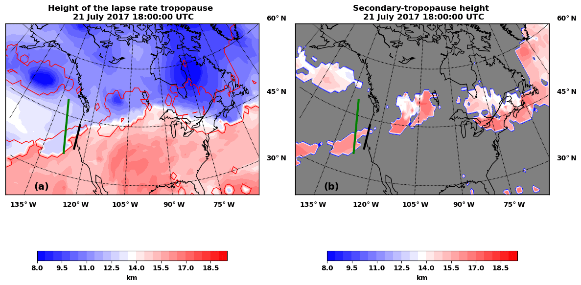
Figure 4Height of the thermal tropopause (a) and the height of the secondary tropopause (b) for the 18:00 UTC time step. The red outline in (a) denotes the edge of the double-tropopause regions shown in (b). The measurement tracks of SHOW and MLS are shown in black and green respectively.

We begin the analysis of SHOW water vapour measurements with three example profiles, shown in Fig. 5a–c, which correspond to the latitude bins centered at 37.4, 41.87, and 43.48^∘ N respectively. Each example shows the set of 10 samples obtained within each latitude bin (black) and the mean of the sample set (red). The observed variance in the water vapour distribution closely matches the 1–2 ppm measurement error predicted by propagating the noise through the retrieval. The red error bars show the precision for the averaged measurements, which is less than < 0.3 ppm for most measurement altitudes. The upper and lower boundaries of the retrievals presented in this paper are 18 km and 13.5 km respectively. The altitude of the first and second lapse rate tropopause are shown as blue solid and dashed lines respectively.

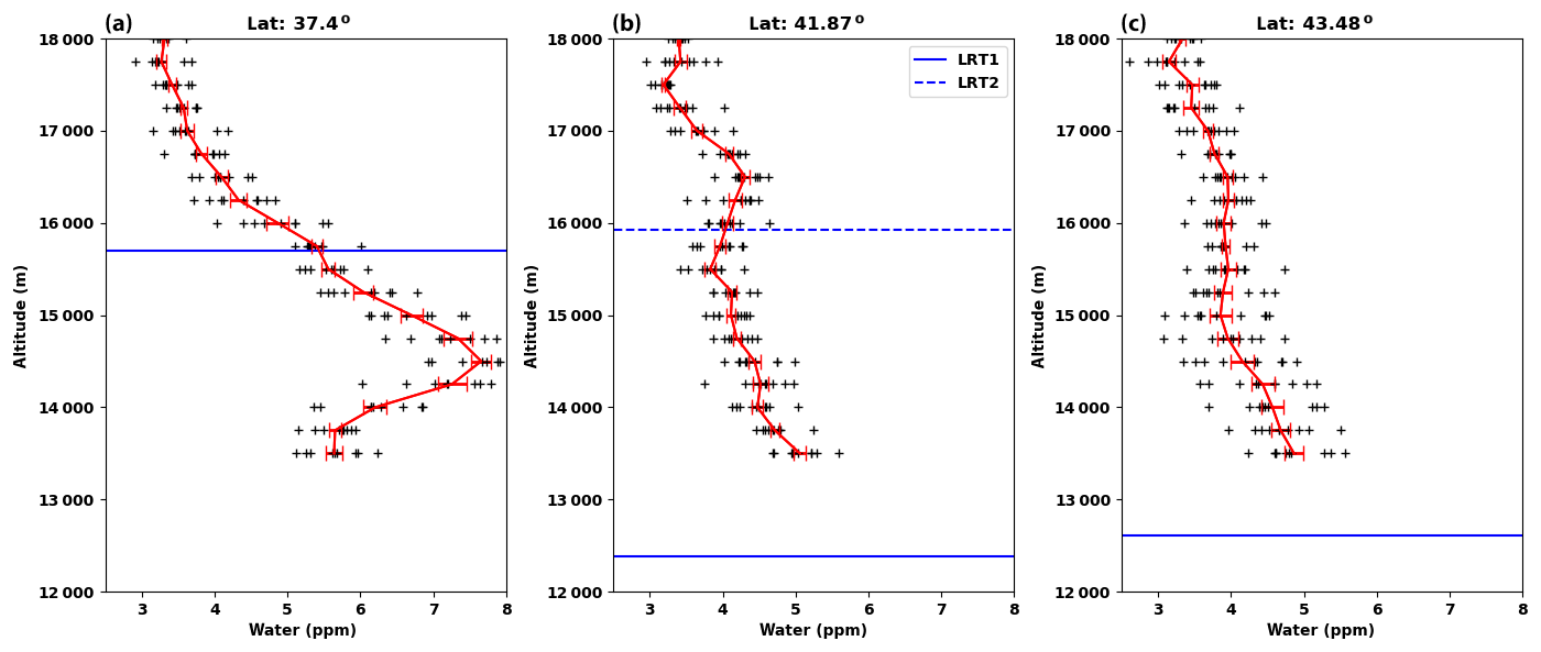
Figure 5Example SHOW profiles at 37.4 (a), 41.87^∘ N (b), and 43.48 (c). All profiles lie closely along the 124.5^∘ W longitude line. The black data points correspond to each of the individual profiles, and the red line is the average of all latitude measurements in each altitude bin. The error bars show the precision of the averaged measurements. The first and second tropopause are identified as the solid blue and dotted blue lines respectively.

Download

For the 37.4^∘ N measurement, the water vapour mixing ratio increases to a maximum near 14.5 km and then decreases rapidly with increasing altitude. The water vapour mixing ratio is also found to decrease slightly below 14.6 km. In the current analysis, the lower boundary of the retrieval is at 13.5 km and therefore does not capture the expected increase of water vapour at altitudes below 13.5 km. At 41.87^∘ N a secondary peak in the water vapour profile is observed near 16.5 km. The amount of water vapour decreases slightly below this peak and then continues to steadily increase with decreasing altitude. Further along the flight track, at 43.48^∘ N, the peak at 16.5 km diminishes and the amount of water vapour increases slowly with decreasing altitude.

Figure 6SHOW-measured water vapour profile (from 18:00 to 19:00 UTC) (a) and the potential-temperature lapse rate determined from the ERA5 reanalysis for the 19:00 UTC time step along the SHOW measurement track (b). The dark dotted line shows the location of the thermal tropopause. The grey contours show the potential vorticity; several zonal wind contours are shown in black; and the light black dotted line shows the 340, 380, and 410 K isentropes respectively. The longitude is along the 124.5^∘ W line and is nearly constant for the measurements.

Download

All of the measured water vapour profiles obtained along the flight track are stacked and plotted as a single data curtain in Fig. 6a. Along this track, SHOW obtained high-vertical-resolution (< 250 m) measurements of UTLS water vapour around the tropopause (13–18 km). These measurements were then averaged by latitude to increase the signal-to-noise ratio, resulting in an along-track sampling of approximately 0.32^∘ latitude. The result provides a high-vertical-resolution time–height (latitude–height) cross section of the water vapour distribution along the flight track. The dynamical fields, including zonal wind, potential vorticity, and the derived tropopause locations from the ECMWF ERA5 reanalysis (19:00 UTC time step), are overlaid on top of the water vapour measurements. The dynamical structure in the cross section co-located with the flight track is further examined in Fig. 6b, where the structure of the static stability is highlighted using the potential-temperature lapse rate (PTLR) determined from the reanalysis data (PTLR $=\mathrm{\Delta }\mathit{\theta }{/}_{\mathrm{\Delta }z}$). In both panels, the 340, 380, and 410 K isentropes are shown as the thin dotted lines, and the thick black dots identify the location of the thermal tropopause.

The 410 K isentrope lies entirely in the stratosphere (in the overworld) at all latitudes. Above the 410 K isentrope, the water vapour mixing ratio is observed to have values between 3.0 and 4.0 ppm, which defines the background water vapour mixing ratio in the lowermost stratosphere. Near the tropopause (in the middle world), sharp spatial structures are resolved that have gradients on the order of 0.5 ppm per 250 m sampling bin. SHOW does not record the water vapour distribution below the 340 K isentrope, since the retrieval cuts off at an altitude of 13.5 km. Discussion of this lower boundary is presented in Sect. 6.

The dynamical structure of the cross section identifies the flight track extended over a well-defined tropopause break over the jet core, which is indicated by tight zonal wind contours (black) near 39.9^∘ N. South of 39.9^∘ N, the thermal tropopause is located at an altitude of close to 15.5 km. The region of 39.9 to 42^∘ N has a double-tropopause structure. More importantly, the region of the tropopause break has a layered structure of static stability, showing a layer of low-stability, troposphere-like air mass extending poleward over the primary tropopause. Consistent with the stability structure, the PV field (grey) in the region shows a weakened gradient. Overall, the dynamical background has a large similarity with the observed tropospheric intrusion from the HIRDLS satellite ozone case study (Fig. 1 in Pan et al., 2009).

Water vapour measurements from SHOW (Fig. 6a) recorded a layer with a water vapour mixing ratio greater than 5 ppmv, which is much higher than the stratospheric background, centered at roughly 14.6 km, and extends poleward to about 40.5^∘ N above the local primary tropopause. Note that the layer in between the two tropopauses where the PV distribution shows a weakened gradient between the 4 and 8 PVU contours indicates a weakened tropopause (Pan et al., 2009; Kunz et al., 2011a, b). Further poleward, the SHOW measurements captured part of a layer with enhanced water vapour above the primary tropopause between 41.5 and 43.5^∘ N. The moist layer is also co-located with the weakened PV gradient.

While the static stability structure of the cross section (Fig. 6b) indicates a case of intrusion of low-static-stability air from the subtropical troposphere into the mid-latitude lowermost stratosphere, the quasi-isentropic transport indicated by the SHOW water vapour cross section does not entirely match the stability structure. Considering that the observation is made in the advent of the Rossby wave-breaking event, it is physically reasonable that the dynamical field and chemical structure are no longer intact, which is a sign of irreversible transport. It is also likely due to the ERA5 products available to the analysis that are given in much coarser vertical resolution compared to the SHOW measurements. The important point is that there is a clear process identification supported by both the water vapour measurement and the dynamical field analysis. We see a similar shift in the analysis of the MLS water vapour and ozone data in the following section.

For additional process verification, we examine measurements of water vapour and ozone that were obtained along a nearly coincident measurement track as shown in Fig. 1 (solid green line). The AURA–MLS satellite instrument obtained measurements along this track at approximately 21:50 UTC – roughly 2 h after the SHOW measurements were performed. Along this track, the MLS instrument sampled the same geophysical feature along a slightly different path with a horizontal resolution of 168–230 km and a vertical resolution of 1.3–3.2 km in the UTLS (316–46 hPa) (Livesey et al., 2018). The MLS measurements have a coarser spatial resolution, and the sampling is not exactly coincident with SHOW. Therefore, some differences are expected between the measurements. However, both sensors sample nearly the same region in the vicinity of the subtropical jet. Therefore, the MLS measurements are used to check for consistency with the meteorological picture in comparison with the SHOW measurements.

The AURA–MLS measurements of water vapour and ozone are shown in Fig. 7a and b respectively. The corresponding PTLR plot is shown in Fig. 7c. For this comparison we use the 22:00 UTC time step of the ECMWF ERA5 reanalysis, since it is the closest available time step to the MLS measurements which occurred at close to 21:50 UTC.

The distributions of the two trace species have a spatial structure that matches the general shape of the structure observed in the PTLR plot and PV contours. As expected, the vertical distributions of the trace species are basically inverted, with water vapour decreasing with increasing altitude and vice versa for ozone. Most importantly, a filamentary structure is observed that extends from 36 to 42^∘ N near 16 km and coincides with the presence of a double tropopause. Again, the feature matches a similar structure that is observed in the corresponding PTLR plot and PV contours at a lower altitude (∼15 km).

Taking the sharpest gradient in the PTLR to define the boundary between tropospheric and stratospheric air, we see that tropospheric air is primarily characterized with a PTLR < 12 K km⁻¹ and stratospheric air is characterized with a PTLR > 12 K km⁻¹. Therefore, as was the case with the SHOW measurements, the observed filamentary structure with a PTLR < 12 K km⁻¹ is consistent with the intrusion of a low-static-stability air from the subtropical troposphere into the mid-latitude lower stratosphere. Mixing on the poleward side of the subtropical jet results in moistening and diminished ozone in the lowermost stratosphere.

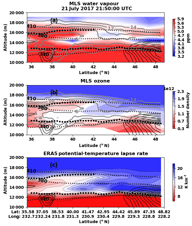
Figure 7MLS-measured water vapour profile (a), ozone (b), and the potential-temperature lapse rate determined from the ERA5 reanalysis for the 22:00 UTC time step along the MLS measurement track (c).

Download

The spatial structures recorded by SHOW (Fig. 6) and MLS (Fig. 7) during this event are strikingly similar and are consistent with spatial structures in the meteorological fields. A direct comparison shows that both instruments recorded similar amounts of water vapour in the vicinity of the subtropical jet. They both capture the moist filament near 16 km as well as the dry regions near 14 km in the lower-latitude portion of the measurement tracks. However, the coarser vertical resolution of MLS smears the vertical extent of the moist filament across a large vertical range of ∼2 km.

Interestingly, the spatial structures observed in the MLS ozone and water vapour profiles are both shifted to a higher altitude relative to the PTLR and PV structures. Regardless, it is clear that the spatial variability observed in the MLS ozone and water vapour measurements, in light of the higher-resolution SHOW observations, is consistent with isentropic mixing on the poleward side of the subtropical jet in the presence of a double tropopause.

The ERA5 reanalysis product was downloaded from the Copernicus Climate Data Store: https://cds.climate.copernicus.eu/cdsapp#!/dataset/reanalysis-era5-pressure-levels (last access: 1 October 2019). The AURA–MLS version 4.2 water vapour and ozone data utilized in this paper were downloaded from the GES-DISC link found at https://mls.jpl.nasa.gov/data/ (last access: 5 April 2019). SHOW data utilized in this paper are available upon request from the author.

JL and AB conceived this study and led the measurement campaign. JL led the interpretation of the measurements and writing of the paper, with significant contributions from LLP. BS is the originator of the instrumentation and contributed to the measurement campaign. DL and DZ made important contributions to the analysis. DD and AB are co-investigators of the project.

The authors declare that they have no conflict of interest.

This research has been supported by the Canadian Space Agency through the Space Technology Development Program.

This paper was edited by Farahnaz Khosrawi and reviewed by two anonymous referees.