2.1 Site description

In order to observe the atmospheric O₂ and CO₂ concentrations and CO₂ flux between the urban area and the overlaying atmosphere, the instruments were installed on a roof-top tower of Tokai University (52 m above ground, 25 m above roof) at Yoyogi (YYG; 35.66^∘ N, 139.68^∘ E), Tokyo, Japan. The YYG site is a mid-rise residential area and located in the northern part of Shibuya ward, Tokyo. Figure 1 shows the location of the YYG site and the flux footprints averaged for summer and winter runs, calculated by the model of Neftel et al. (2008). The main land cover around the site is characterized by low- to mid-rise residential buildings with a mean height of 9 m. The population density in this area is 16 600 persons per square kilometer. At the YYG site, the prevailing wind is from SW in the summer and NW in the winter. The flux footprint includes a vegetated area of 9 % in the summer and 2 % in the winter, reflecting seasonal changes in the wind direction.

Figure 1(a) Location of the Yoyogi site (35.66^∘ N, 139.68^∘ E, YYG), Tokyo, Japan. (b, c) Aerial photo from the Geospatial Information Authority of Japan around the study area at YYG. Ensemble-mean flux footprints in the summer (b) and winter (c) are also shown by black circles. The contour lines indicate contribution in measured flux (60 %, 50 %, 40 %, 30 %, 20 % and 10 % from outside to inside). Inside and outside the red circles indicate the distances of 500 and 1000 m, respectively, from a roof-top tower of Tokai University where the observations of O₂ and CO₂ concentrations and CO₂ flux were carried out.

2.2 Continuous measurements of the atmospheric O₂ and CO₂ concentrations and CO₂ flux

Observations of the atmospheric O₂ and CO₂ concentrations have been carried out at the YYG site using a continuous measurement system employing a paramagnetic O₂ analyzer (POM-6E, Japan Air Liquid) and a non-dispersive infrared CO₂ analyzer (NDIR; Li-820, LI-COR) since March 2016. The O₂ concentration is reported as the O₂∕N₂ ratio in per meg:

where the subscripts “sample” and “standard” indicate the sample air and the standard gas, respectively. Because O₂ is about 20.94 % of air by volume (Tohjima et al., 2005a), the addition of 1 µmol of O₂ to 1 mol of dry air increases δ(O₂∕N₂) by 4.8 per meg ($=\mathrm{1}/\mathrm{0.2094}$). If CO₂ were to be converted one-for-one into O₂, this would cause an increase of 4.8 per meg of δ(O₂∕N₂), equivalent to an increase of 1 µmol mol⁻¹ in O₂ for each 1 µmol mol⁻¹ decrease in CO₂. Therefore, the ratio of 4.8 per meg µmol mol⁻¹ was used to convert the observed δ(O₂∕N₂) to O₂ concentration relative to an arbitrary reference point. In this study, δ(O₂∕N₂) values of each air sample were measured with the paramagnetic analyzer using working standard air that was measured against our primary standard air (cylinder no. CRC00045; AIST scale) using a mass spectrometer (Thermo Scientific Delta-V) (Ishidoya and Murayama, 2014).

Sample air was taken at the tower heights of 52 and 37 m using a diaphragm pump at a flow rate higher than 10 L min⁻¹ to prevent thermally diffusive fractionation of air molecules at the air intake (Blaine et al., 2006). Then, a large portion of the air is exhausted from the buffer, with the remaining air allowed to flow into the analyzers from the center of the buffer. It is then sent to an electric cooling unit with a water trap cooled to −80 ^∘C at a flow rate of 100 mL min⁻¹, with the pressure stabilized to 0.1 Pa and measured for 10 min at each height (one-cycle measurements). The method to sample a small subset of air from a high flow rate is similar to those used in Goto at el. (2013b), and we have confirmed that the atmospheric δ(O₂∕N₂) values observed by the measurement system agree well with those obtained from independent continuous measurements of δ(O₂∕N₂) using the mass spectrometer (see Fig. 4 in Ishidoya et al., 2017). After nine cycles of measurements (five and four cycles for 37 and 52 m, respectively), high-span standard gas, prepared by adding appropriate amounts of pure O₂ or N₂ to industrially prepared CO₂ standard air, was introduced into the analyzers with the same flow rate and pressure as the sample air and measured for 5 min, and then low-span standard gas was measured by the same procedure. The dilution effects on the O₂ mole fraction measured by the paramagnetic analyzer were corrected experimentally, not only for the changes in CO₂ of the sample air or standard gas measured by the NDIR, but also for the changes in Ar of the standard gas measured by the mass spectrometer as δ(Ar∕N₂). The analytical reproducibility of the δ(O₂∕N₂) and CO₂ concentration achieved by the system was about 5 per meg and 0.06 µmol mol⁻¹, respectively, for 2 min average values. Details of the continuous measurement system used are given in Ishidoya et al. (2017).

It should be noted that we used the gravimetrically prepared air-based CO₂ standard gas system with uncertainties of ±0.13 µmol mol⁻¹ on the TU-10 scale (Nakazawa et al., 1991) to determine CO₂ concentration in this study. The highest concentration of the gravimetrically prepared standard gas was about 450 µmol mol⁻¹, while CO₂ concentrations of more than 600 µmol mol⁻¹ were observed in this study. Therefore, we compared the NDIR-based CO₂ concentrations observed in this study with those observed by using cavity ring-down spectroscopy (CRDS; G2401, Picarro) on the NIES-09 scale (Machida et al., 2011) at the YYG site (our unpublished data). Although the highest CO₂ concentration of the gravimetrically prepared standard of the NIES-09 scale is similar to that of the TU-10 scale, a slope of 0.974 ppm ppm⁻¹ is derived from a least-squares regression line fitted to the relationship between the CO₂ concentrations observed by NDIR on the TU-10 scale and those by CRDS on the NIES-09 scale with a correlation coefficient (r) of 0.978. On the other hand, we obtained a slope of 1.002 per meg per meg⁻¹ (r=0.999) from the regression line fitted to the relationship between the O₂ concentrations of gravimetrically prepared standard gases (Aoki et al., 2019) measured by the mass spectrometer on the AIST scale and the gravimetric values of the standard gases covering a much wider range than the atmospheric variations in the O₂ concentration. Therefore, the uncertainty in OR due to the span uncertainties of O₂ and CO₂ concentrations is expected to be within 3 %.

In order to observe the CO₂ flux at the YYG site, the turbulence and the turbulent fluctuation of CO₂ were observed at 52 m with a high time resolution of 10 Hz by using a sonic anemometer (WindMasterPro, Gill) and an open-path infrared gas analyzer (LI-7500, LI-COR) starting November 2012. The sensors were located at more than 5 times the mean building height (9 m), and then it was above the urban roughness sublayer. Turbulent flux of CO₂ was calculated by the eddy correlation method using EddyPro^® (Licor) for every 30 min period. Correlations were applied in the calculation for water-vapor density fluctuation (Webb et al., 1980) and mean vertical wind by using the double rotation algorithm (Wilczak et al., 2001). The calculated flux was filtered for data quality based on the steady test and the integral turbulence characteristics in Aubinet et al. (2012). We used the flag 0–2 data in EddyPro^® software based on Mauder and Foken (2006).

3.1 Variations in the atmospheric O₂ and CO₂ concentrations

We show the 10 min average values of the atmospheric O₂ and CO₂ concentrations observed at the height of 52 m at YYG in Fig. 2. As seen in the figure, O₂ and CO₂ concentrations vary in opposite phase with each other on timescales ranging from several hours to a seasonal cycle. In general, opposite phase variations of atmospheric O₂ and CO₂ are driven by fossil fuel combustion and terrestrial biospheric activities. In contrast, the atmospheric O₂ variation in µmol mol⁻¹ due to the air–sea exchange of O₂ is much larger than that of CO₂ on timescales shorter than 1 year (e.g., Goto et al., 2017; Hoshina et al., 2018); this is because the equilibration time for O₂ between the atmosphere and the surface ocean is much shorter than that for CO₂ due to the influence of the carbonate dissociation effect on the air–sea exchange of CO₂ (Keeling et al., 1993). Therefore, we attribute the opposite phase variations in O₂ and CO₂ observed in this study mainly to fossil fuel combustion and terrestrial biospheric activities. Figure 2 also shows that ΔO₂, obtained by subtracting O₂ at 41 m from that at 52 m on the tower, varies in opposite phase with the corresponding ΔCO₂. High ΔO₂ values are more frequently observed in the winter than in the summer, and short-term (several hours to days) decreases in the O₂ concentration are intense in the winter.

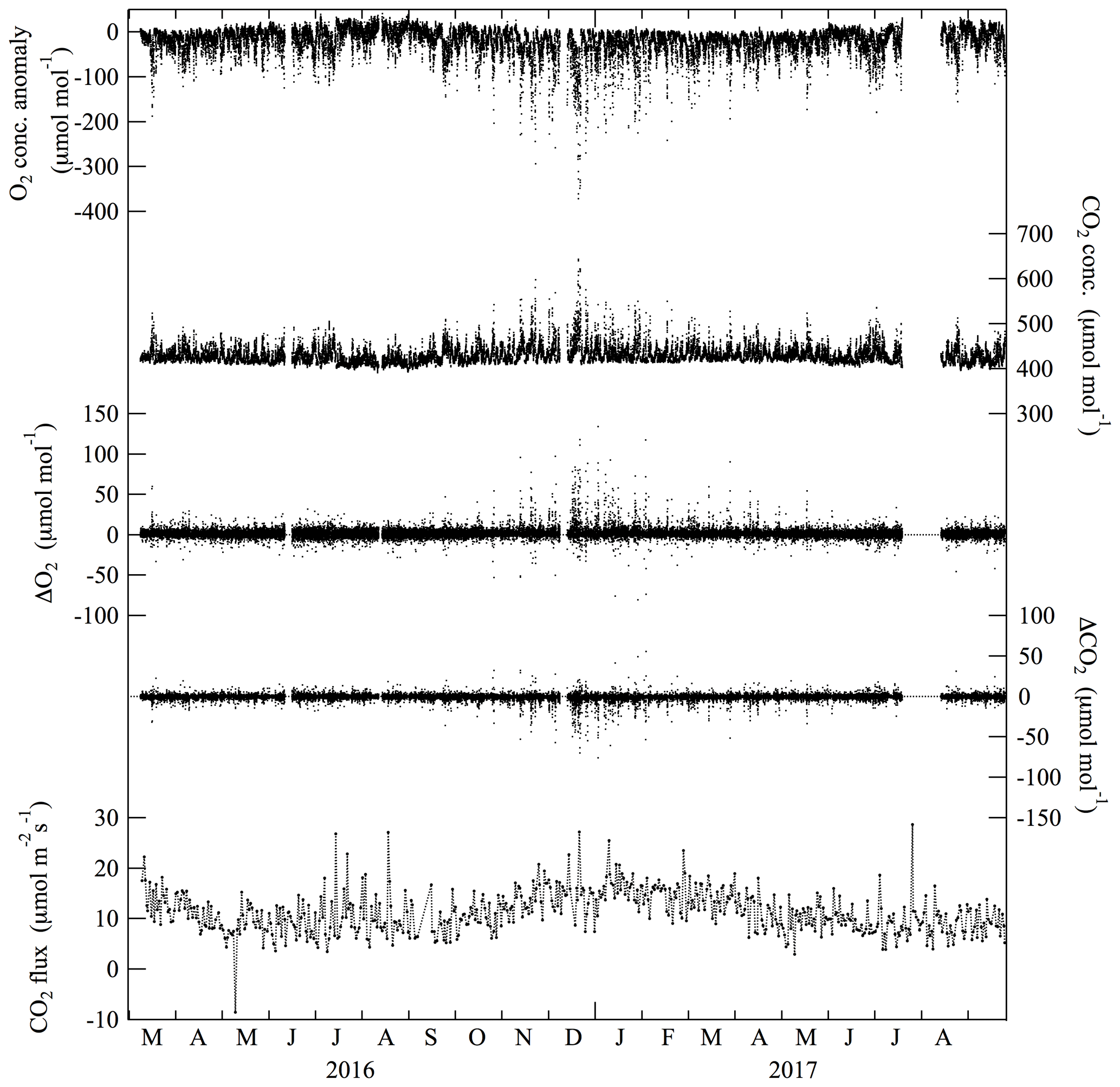
Figure 2Variations in O₂ and CO₂ concentrations observed at the tower height of 52 m at Yoyogi, Tokyo, Japan, for the period March 2016–September 2017. The O₂ concentrations are expressed as deviations from the value observed at 09:58 local time on 9 March 2016. ΔO₂, representing the differences calculated by subtracting the observed O₂ concentrations at 37 m from that at 52 m, are also shown. ΔCO₂ are the same as ΔO₂ but for CO₂ concentration. Daily mean CO₂ fluxes observed using the eddy correlation method are also shown, and the flux takes on a positive value when the urban area emits CO₂ to the overlaying atmosphere.

Download

To examine a relationship between the appearances of high ΔO₂ and O₂ concentration decrease, detail variations in the O₂ and CO₂ concentrations, ΔO₂ and ΔCO₂ for the periods 16–23 December and 1–9 July 2016, are shown in Fig. 3. As seen in the figure, increases in ΔO₂ coincide with decreases in O₂ concentration in December, especially in the nighttime. Such a coincidence is also seen in July; however, the increases in ΔO₂ are much smaller than those in December. Therefore, it is highly likely that O₂ is consumed within the urban canopy at YYG, more so in the winter due to an increased usage of gas and/or liquid fuels for heating and to a temperature inversion near the surface. The daily mean CO₂ flux from the urban area to the overlaying atmosphere shown in Fig. 2 shows a seasonal cycle with a wintertime maximum, consistent with the enhancement of O₂ consumption in the urban canopy.

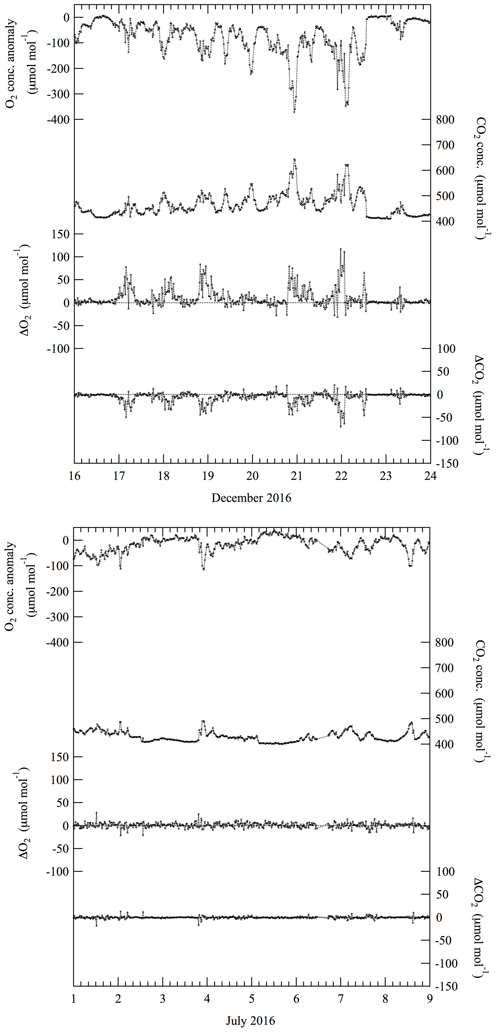
Figure 3Same as in Fig. 2 but for O₂ and CO₂ concentrations, ΔO₂ and ΔCO₂ for the periods 16–23 December and 1–9 July 2016.

Download

In this study, we focus on the short-term variations of O₂ and CO₂ for periods of several hours to days, to elucidate the O₂ and CO₂ exchange processes between the urban area and the atmosphere by examining two types of OR: one is OR_atm calculated from a relationship between the O₂ and CO₂ concentration values observed at 52 or 37 m and the other one is OR_F, for the O₂ and CO₂ fluxes between the urban area and the overlaying atmosphere, calculated from a relationship between ΔO₂ and ΔCO₂. The relationships of the O₂ and CO₂ fluxes with OR_F are based on the aerodynamic method of Yamamoto et al. (1999):

Here, F_O (F_C) (µmol m⁻² s⁻¹) represents the O₂ (CO₂) flux from the urban area to the overlaying atmosphere, K is the vertical diffusion coefficient, and ΔO₂Δz⁻¹ (ΔCO₂Δz⁻¹) is the vertical concentration gradient of O₂ (CO₂). The vertical diffusion is a sum of mass-independent eddy and mass-dependent molecular diffusion; however, the effect of molecular diffusion on the observed variations of O₂ and CO₂ concentrations is generally negligible in the troposphere. It is significant in the stratosphere (e.g., Ishidoya et al., 2013a). Therefore, we used the same diffusion coefficient K for O₂ and CO₂ in Eqs. (2) and (3), which enabled us to estimate F_O by using the observed ΔO₂, ΔCO₂ and F_C as in Eq. (4). In general, OR_atm reflects wider footprints of O₂ and CO₂ than OR_F due to horizontal atmospheric transport (Schmid, 1994). We note that the definitions of OR_F and OR_atm are similar to those of ER_F and ER_atm, respectively, reported by Ishidoya et al. (2013b, 2015).

In order to calculate OR_atm for short-term variations, (1) we applied a best-fit curve consisting of the fundamental and its first harmonics (periods of 12 and 6 months) and a linear trend to the maximum (minimum) values of O₂ (CO₂) observed at 52 m during the successive 1-week periods and regarded the best-fit curve as its baseline variation; (2) then, the baseline variation of O₂ (CO₂) concentration was subtracted from the respective O₂ (CO₂) concentrations observed at 52 m. Figure 4 shows the baseline variations and the variations in the O₂ and CO₂ concentrations observed at Minamitorishima (MNM; 24.28^∘ N, 153.98^∘ E), Japan (updated from Ishidoya et al., 2017). MNM is a small and isolated coral island located 1850 km southeast of Tokyo, Japan, and the observation site was operated by the Japan Meteorological Agency (JMA) under the Global Atmosphere Watch program of the World Meteorological Organization (WMO/GAW). The baseline variations of O₂ and CO₂ at YYG show clear seasonal cycles with peak-to-peak amplitudes of 28 and 16 µmol mol⁻¹, respectively, with a corresponding seasonal maximum and minimum appearing in mid August. The amplitude of the seasonal O₂ (CO₂) cycle and the appearance of a seasonal maximum (minimum) were found to be larger and earlier, respectively, than those observed at MNM, while the annual average values of the baseline concentration variations of O₂ and CO₂ at YYG did not differ significantly from those at MNM. These characteristics of the seasonal cycles and the annual average values of the baseline variations at YYG and their comparison with those at MNM are generally consistent with those observed at similar latitude over the western Pacific region (Tohjima et al., 2005b). Therefore, in spite of the fact that the YYG site is located in a megacity, the baseline variations of O₂ and CO₂ concentrations are similar to those in the background air.

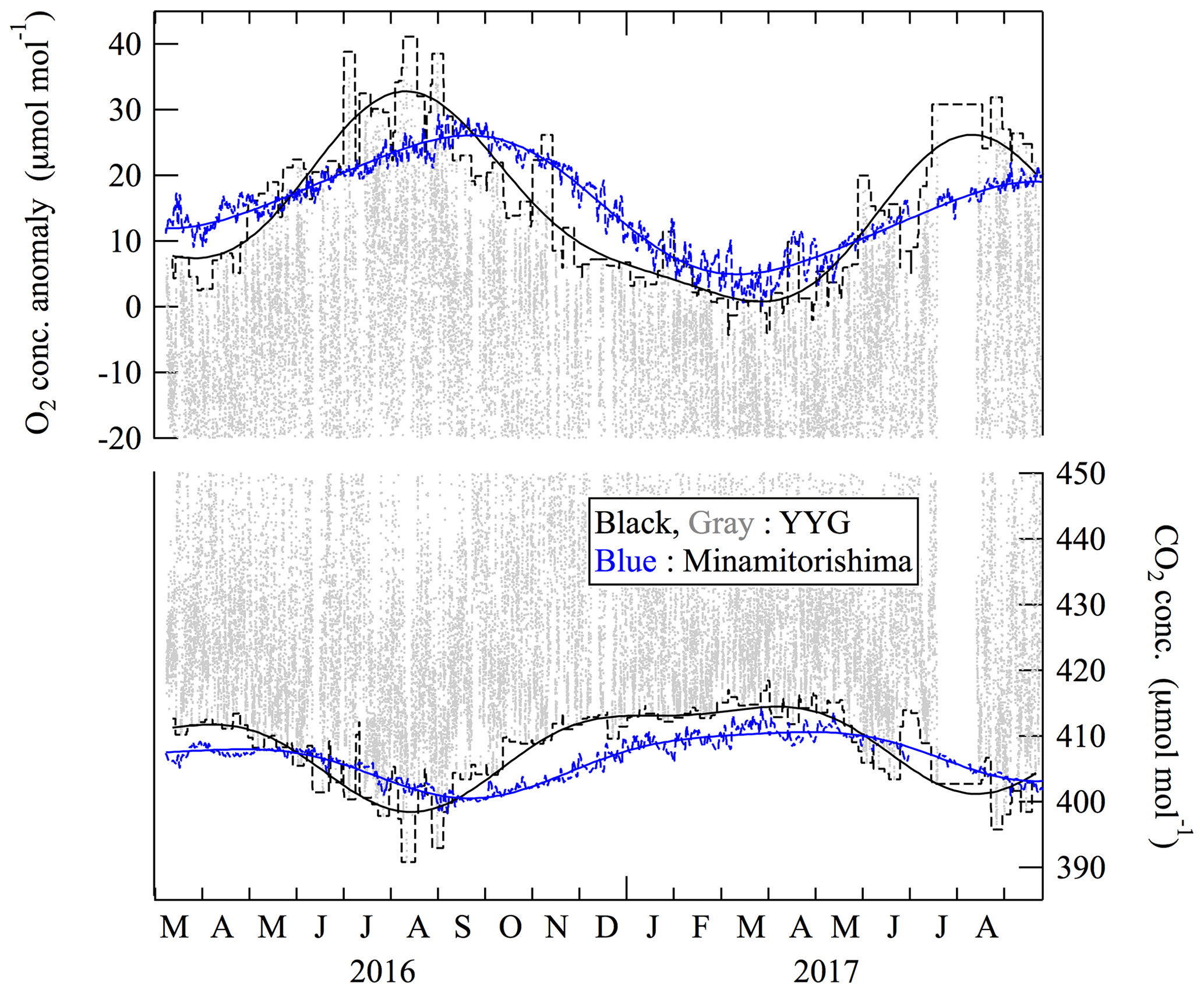
Figure 4Baseline variations of O₂ and CO₂ concentrations at the tower height of 52 m at Yoyogi, Tokyo, Japan, represented by their best-fit curves (black solid lines) to the respective maximum and minimum values during the successive 1-week periods (black dashed lines). Variations of 24 h averaged O₂ and CO₂ concentrations at Minamitorishima, Japan (blue dashed line), and their best-fit curves (blue solid lines), are also shown (updated from Ishidoya et al., 2017).

3.2 O₂ : CO₂ exchange ratio between the urban area and the overlaying atmosphere

Figure 5a shows the relationship between all the ΔO₂ and ΔCO₂ values to obtain the average OR_F throughout the observation period in this study. When errors in both species are non-negligible, a standard least-squares linear regression will give a biased and erroneous slope. Therefore, we apply an unweighted Deming regression analysis to the data (e.g., Linnet, 1993), assuming the ratio between the squared analytical standard deviations to be ${\mathrm{0.06}}^{\mathrm{2}}/{\left(\mathrm{5}\times \mathrm{0.2094}\right)}^{\mathrm{2}}$ (ppm ppm⁻¹) to take into account the measurement uncertainties of CO₂ and O₂ concentrations. We consider the slope obtained by Deming regression to be OR_F, but we use a standard deviation obtained from a standard least-squares regression to indicate the uncertainty of the slope. The jackknife method (Linnet, 1990) could be used to derive a standard error for Deming regression; however, by using a short dataset extracted from the observed data used in the present study, we confirmed that the standard deviations obtained from an ordinary regression are larger than the errors from the jackknife method. Therefore, using a standard deviation from ordinary regression is reasonable to ensure larger uncertainty for the OR_F. The average OR_F value was calculated to be 1.620±0.004 (±1σ). This value falls within the range of the average OR values of 1.44 for liquid fuels and 1.95 for gas fuels, which suggests that the O₂ and CO₂ fluxes at the YYG site were driven mainly by a consumption of liquid and gas fuels rather than terrestrial biospheric activities of which OR is about 1.1 (Severinghaus, 1995). The relationship between the O₂ and CO₂ concentration anomalies, calculated by subtracting the respective baseline variations shown in Fig. 4 from the observed O₂ and CO₂ concentrations, is also shown in Fig. 5b. By applying the Deming regression analysis to the data, we obtained an average OR_atm value of 1.541±0.002 (±1σ) throughout the observation period. The OR_atm value also falls within the range of the average OR values for liquid fuels and gas fuels. However, the OR_atm in this figure is not appropriate in representing the OR for the O₂ and CO₂ fluxes around the YYG site since it was determined by using the entire 18 months of collected observations that the site is influenced by various trajectories of air masses with a much wider regional signature than the flux footprints. Therefore, we compare below the OR_F and OR_atm values by changing the aggregation periods to calculate the ORs and examine the validity of using OR_F rather than OR_atm to evaluate the relationship between the local O₂ and CO₂ fluxes.

Figure 5(a) Relationship between the ΔO₂ and ΔCO₂ shown in Fig. 2. The average OR_F (see text) for the observation period, derived from the Deming regression fitted to the data, is also shown. (b) Same as in (a) but for the deviations of O₂ and CO₂ concentrations from their baseline variations shown in Fig. 3 and the average OR_atm (see text). OR values expected from the consumptions of gas and liquid fuels are also shown.

Download

Figure 6 shows examples of the OR_F calculated by applying Deming regression fitted to ΔO₂ and ΔCO₂ values during the successive 12 h periods observed in January 2017 and July 2016. The corresponding OR_atm and wind direction observed for the periods are also shown in the figure. As seen in the figure, variabilities in the OR_F and OR_atm are larger in July than in December. The average OR_F, calculated using the OR values within a range of 0.5 to 2.5, were 1.65±0.20 and 1.52±0.32 in the winter (December to February) and summer (July to September), respectively. The corresponding average OR_atm values were 1.61±0.15 in the winter and 1.45±0.27 in the summer. To examine the dependency of the OR on the wind direction, we also calculated OR_F and OR_atm for the periods when the prevailing wind directions were observed to be from 320 to 360^∘ (NW) and from 180 to 220^∘ (SW) in the winter and summer, respectively. The number of measurements taken during the time of these prevailing winds constituted 30 % (winter) and 8 % (summer) of the total number of measurements. The calculated OR_F, OR_atm and prevailing winds are shown by blue dots in Fig. 6. The average OR_F (OR_atm) values, calculated using the OR values within a range of 0.5 to 2.5, were 1.65±0.25 (1.58±0.19) in the winter and 1.58±0.40 (1.42±0.33) in the summer, respectively. Therefore, the average OR_F and OR_atm calculated using all the values obtained from the 12 h aggregation periods did not differ significantly from those that were calculated using only the data that were associated with the above-mentioned prevailing wind directions. The average OR_F seems to be slightly higher than OR_atm; however, their uncertainties are too large to discuss the significance of the slight difference. Taking these facts into consideration, we use all the O₂ and CO₂ concentration data without filtering by the wind direction to increase the number of data points for calculating OR_F and OR_atm; this is consistent with the purpose of this study to derive representative OR values at the YYG site in order to validate the CO₂ emission inventory (Hirano et al., 2015). For analyses of specific events, we have reported analytical results of OR_atm and simultaneously measured PM_2.5 aerosol composition for a week long pollution event at the YYG site (Kaneyasu et al., 2020).

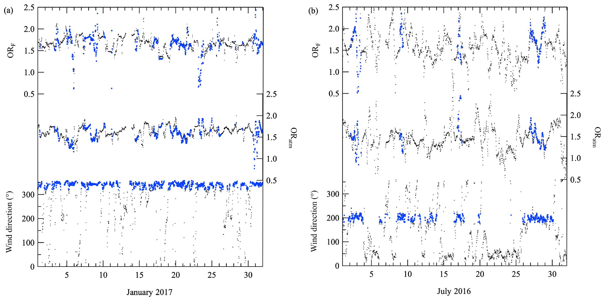
Figure 6(a) OR_F (black dots, top) calculated by applying Deming regression fitted to ΔO₂ and ΔCO₂ values during the successive 12 h periods observed in January 2017. The corresponding OR_atm (black dots, middle) obtained from the deviations of O₂ and CO₂ concentrations from their baseline variations shown in Fig. 4, and the wind directions (black dots, bottom), are also shown. Angles of 90, 180, 270 and 360^∘ for the wind direction denote winds from east, south, west and north, respectively. The OR_F and OR_atm obtained from the data observed during the period with the prevailing wind direction (blue dots, bottom) are also shown by blue dots. (b) Same as in (a) but for July 2016.

Download

To examine the seasonal difference between the OR_F and OR_atm values, we show the OR_F values calculated by applying regression lines to 1 d and 1-week successive ΔO₂ and ΔCO₂ values in Fig. 7. The corresponding OR_atm values, obtained by applying Deming regression fitted to successive O₂ and CO₂ concentration anomalies in Fig. 5b, are also shown. Since there is no statistically significant difference between the two (based on the uncertainties shown in the figure (±1σ)), we focus our discussion on the OR values obtained from the 1-week successive data. Clear seasonal cycles with wintertime maxima are found in both the OR_F and OR_atm values at YYG. Larger OR_atm values in the winter than in the summer in urban areas have been reported by some past studies (e.g., van der Laan et al., 2014; Ishidoya and Murayama, 2014; Goto et al., 2013a) and generally interpreted as a result of the wintertime increase and decrease in fossil fuel combustion and terrestrial biospheric activities, respectively. Biospheric activities included in the summertime and wintertime flux footprints at YYG were 9 % and 2 %, respectively (Hirano et al., 2015), and there was no significant solid fuel consumption, such as a coal-fired power-generation plant of which OR is expected to be 1.17 (Keeling, 1988), detected in the footprints. At YYG, the effect of emissions from coal combustion is evaluated simultaneously by the use of aerosol composition monitored every 4 h (Kaneyasu et al., 2020). From these measurements, emission contribution from coal combustion can be detected under a limited meteorological condition, such as a stagnant condition under a weak south-southwesterly wind. This condition occurred only several times a year, mostly from spring to fall. Therefore, the wintertime OR_F was determined mainly by gas and liquid fuel consumption around the YYG site, given that few vegetation and weak terrestrial biospheric activities took place in the wintertime. If we assume the wintertime OR_F is determined only by gas and liquid fuel consumption, with OR values of 1.95 and 1.44, respectively, then 45 % of the CO₂ flux during the December to February (DJF) period was driven by gas fuel consumption, with the rest attributed to liquid fuel consumption. It should be noted that the contributions of gas and liquid fuels are expected to be underestimated and overestimated since we have ignored the contribution from human respiration with OR values in the range of 1.0 to 1.4. The respiration quotients (the reciprocal of OR) for carbohydrates, lipid and protein are known to be about 1.0, 0.7 and 0.8, respectively. We also conducted detail analyses to separate out the contributions from the consumption of gas and liquid fuels and human respiration by using the observed CO₂ flux and OR_F and comparing the results with the CO₂ emission inventory in Sect. 3.3.

Figure 7 also shows that the OR_F values were systematically larger than OR_atm throughout the year, except for October 2016 and July 2017. The average OR_F and OR_atm during DJF were 1.67±0.03 and 1.63±0.02, respectively, both of which agree with the OR value of 1.65 calculated using the statistical data of fossil fuel consumption in Tokyo reported by the Agency of Natural Resources and Energy (http://www.enecho.meti.go.jp/en/, last access: 18 December 2018), assuming OR values of 1.95, 1.44 and 1.17 for gas, liquid and solid fuel consumption, respectively (hereafter referred to as “OR_ff”). By using the same procedure as above, the average OR_ff was calculated to be 1.52±0.1 for the Kanto area of about 17 000 km² that includes Tokyo. Therefore, it is suggested that not only OR_F, but also OR_atm at YYG, mainly reflected an influence of the fossil fuel consumption in Tokyo rather than that in the wider Kanto area in the wintertime. Both the OR_F and OR_atm values in the summer were lower than OR_ff in Tokyo (1.65), but OR_atm was also found to be lower than OR_ff for the Kanto area (1.52). These lower OR_F and OR_atm values, compared to those of the OR_ff, suggest that the ratio of fossil fuel combustion to terrestrial biospheric activities and human respiration is lower in the summer than that in the winter. The slightly lower OR_atm than OR_F at YYG throughout the year is probably due to the higher contribution of the air mass from the Kanto area to OR_atm than OR_F, since the Kanto area as a whole has lower OR_ff than for Tokyo; in addition, the southern Kanto area (including Tokyo) has a larger vegetation coverage of about 50 % than that in the area around the YYG site. From the comparison results of the OR_F with OR_atm in Figs. 5–7, it is suggested that the OR_atm reflects wider footprints of O₂ and CO₂ than OR_F for the aggregation periods at least longer than 12 h to calculate the OR_atm. Therefore, to use OR_F rather than OR_atm is more appropriate to validate inventory-based CO₂ emissions from gas, liquid and solid fuels in the flux footprint.

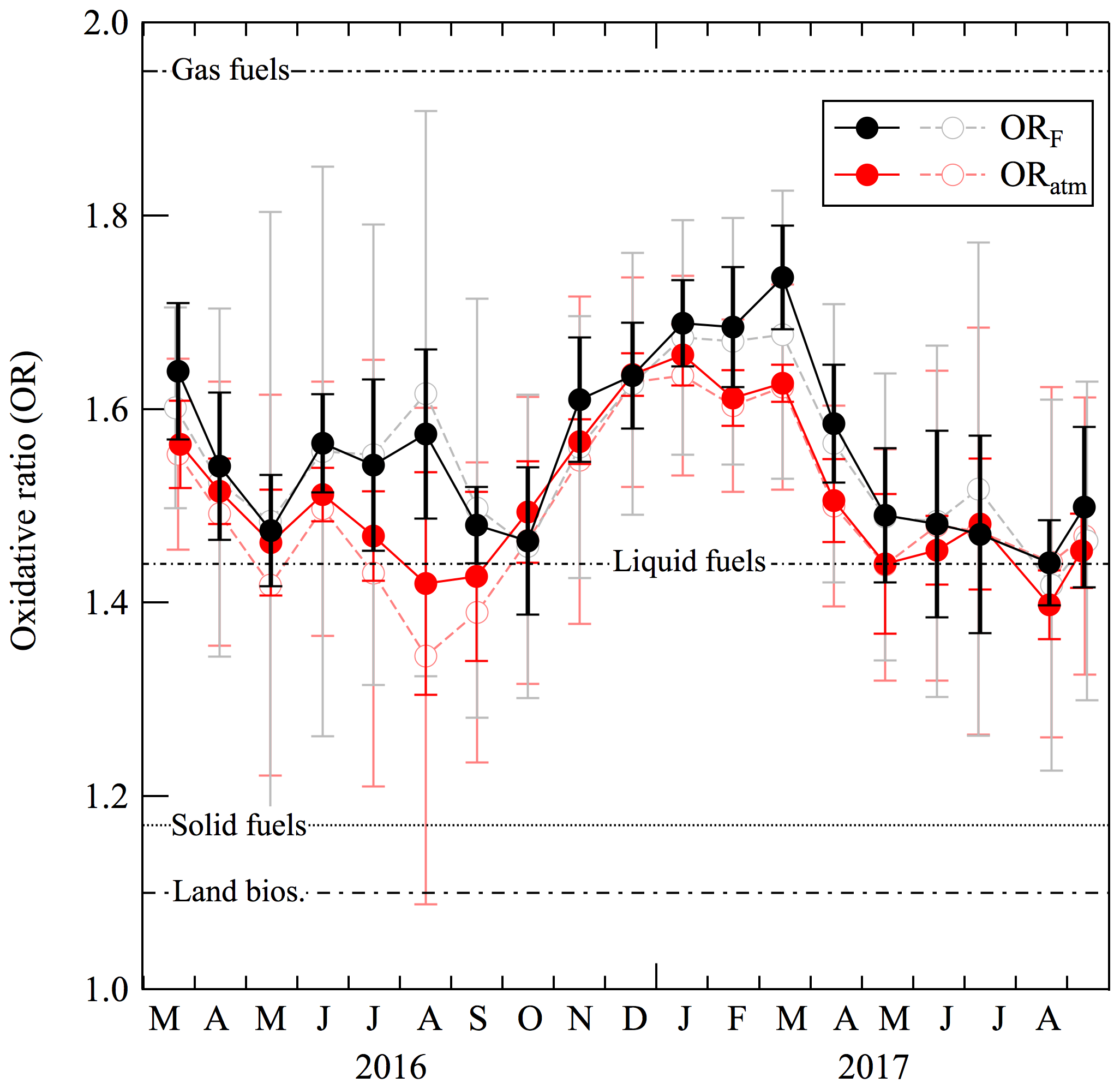
Figure 7OR_F calculated by applying Deming regression fitted to 1 d (gray open circles) and 1-week (black closed circles) successive ΔO₂ and ΔCO₂ values. Also plotted are OR_atm calculated by applying Deming regression fitted to 1 d (light red open circles) and 1-week (dark red closed circles) successive O₂ and CO₂ deviations from their baseline variations shown in Fig. 3. OR values expected from the consumptions of gas, liquid and solid fuels and land biospheric activities are also shown.

Download

3.3 Consumption of gas and liquid fuels estimated from the observed CO₂ flux and O₂ : CO₂ exchange ratio for net turbulent flux

In this section, we derive average diurnal cycles of OR_F, CO₂ and O₂ fluxes and estimate the CO₂ fluxes from gas and liquid fuel consumption separately. Figure 8 shows the average diurnal cycles of ΔO₂ and ΔCO₂ for each season. To derive the average diurnal cycles, the observed ΔO₂ and ΔCO₂ values of each day in a season were overlain on top of the values of other days, added up and divided by the number of days in the season. The error bars shown in Fig. 8 indicate ±1 standard error ($\mathit{\sigma }/\sqrt{n}$). The ΔO₂ and ΔCO₂ values vary systematically in opposite phase and take positive and negative values, respectively, indicating transport of O₂ uptake and CO₂ emission signals from the urban area to the overlaying atmosphere throughout the year. Daily maxima of ΔO₂ shown in Fig. 8 are higher in the winter than in the summer and occur in the nighttime. These characteristics would be attributable to an enhancement of the anthropogenic O₂ consumption in the winter, while the nighttime decrease in O₂ concentration would be due to the O₂ consumption near the surface and temperature inversion near the surface. It must be noted that the ΔCO₂ values in the daytime are nearly zero, while the ΔO₂ values are not. The intercepts of the regression lines fitted to the relationship between ΔO₂ and ΔCO₂ in Fig. 8 are 0.27, 0.41, 0.45 and 0.44 µmol mol⁻¹ in DJF, MAM, JJA and SON, respectively. Unfortunately, we did not fix the cause(s) of such biases yet, although it (they) may be related, to some extent, to natural exchange processes between the urban area and the overlaying atmosphere. Therefore, because of these issues, the use of OR_F, calculated by applying a Deming regression fitted to 2 h period values of ΔO₂ and ΔCO₂ of the climatological diurnal cycle (the number of data included in each 2 h periods were 400–800, depending on the season), to determine the relationship between the O₂ and CO₂ fluxes, is preferable. The OR_F values plotted in Fig. 8 show diurnal cycles with daytime minima in DJF, MAM and SON, while no clear cycle is found in JJA. From 10:00 to 16:00 local time, the OR_F values are in the range of 1.44–1.59 for all seasons. On the other hand, the OR_F values from 18:00 to 09:00 local time are more variable, in the range of 1.39–1.74, and are clearly larger in the winter than in the summer.

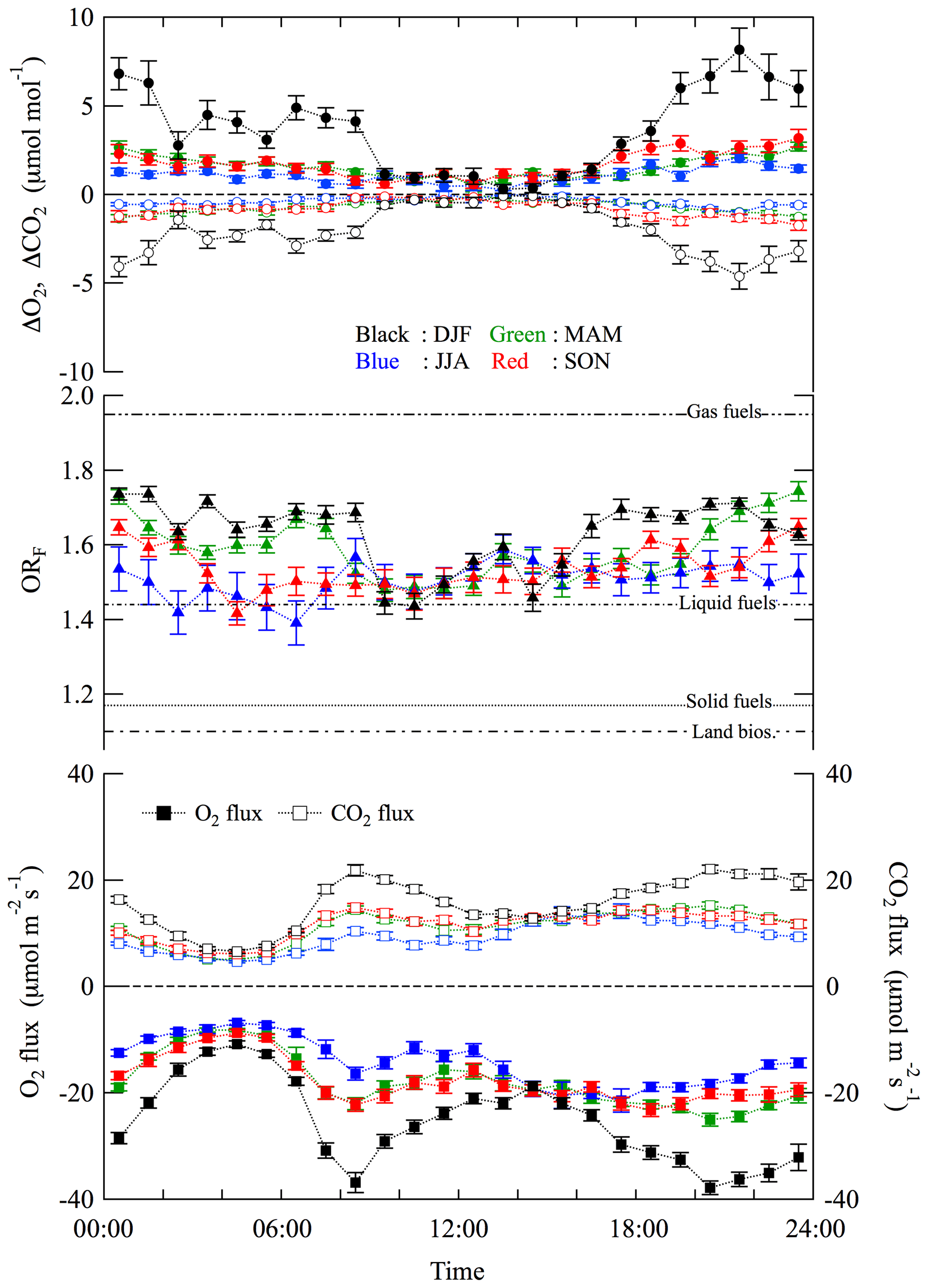
Figure 8Plots of average diurnal cycles of ΔO₂ (filled circles) and ΔCO₂ (open circles) for each season: December to February (back), March to May (green), June to August (blue) and September to November (red). Average diurnal cycles of OR_F, calculated by applying Deming regression fitted to the 2 h period values of ΔO₂ and ΔCO₂, are also plotted seasonally (see text). Average diurnal cycles of the CO₂ flux observed using the eddy correlation method, and those of the O₂ flux calculated from the CO₂ flux and OR_F values, are also plotted seasonally. Error bars indicate ±1 standard error.

Download

The observed CO₂ flux and the estimated O₂ flux for each season are shown in Fig. 8. The CO₂ flux shows clear diurnal cycles with two peaks for all seasons, one in the morning and the other in the evening. The shape of the diurnal CO₂ flux cycle, with larger flux in the winter than in the summer, was also found in our previous study at YYG for the period 2012–2013 (Hirano et al., 2015). On the other hand, the O₂ flux shows similar diurnal cycles but in opposite phase with the CO₂ flux. The daily mean CO₂ fluxes were 15.6±0.2, 11.2±0.1, 9.3±0.1 and 11.5±0.1 µmol m⁻² s⁻¹ in DJF, MAM, JJA and SON, respectively, while the respective daily mean O₂ fluxes were $-\mathrm{25.4}\pm \mathrm{0.3}$, $-\mathrm{17.8}\pm \mathrm{0.2}$, $-\mathrm{14.1}\pm \mathrm{0.2}$ and $-\mathrm{17.7}\pm \mathrm{0.2}$ µmol m⁻² s⁻¹. The annual average daily mean O₂ flux was −16.3 µmol m⁻² s⁻¹. Steinbach et al. (2011) reported a global dataset of CO₂ emissions and O₂ uptake associated with fossil fuel combustion using the EDGAR inventory with country-level information on OR, based on the fossil fuel consumption data from the UN energy statistics database. The O₂ uptake around Tokyo for the year 2006 has been shown to be about e¹⁶–e¹⁷ kgO₂ km⁻² yr⁻¹ (Fig. 2 in Steinbach et al., 2011), which corresponds to −9 to −24 µmol m⁻² s⁻¹ of O₂ flux and is consistent with those observed in this study. In this regard, the atmospheric O₂ concentration decreased secularly due mainly to fossil fuel combustion at a rate of change of about −4 µmol yr⁻¹ (e.g., Keeling and Manning, 2014), corresponding to −0.04 µmol m⁻² s⁻¹ of O₂ flux, assuming 5.1×10¹⁴ m² for the surface area of the earth, 5.124×10²¹ g for the total mass of dry air (Trenberth, 1981) and 28.97 g mol⁻¹ for the mean molecular weight of dry air. Therefore, the consumption rate of atmospheric O₂ in an urban area of Tokyo is several hundred times larger than the global mean surface consumption rate.

The CO₂ emission inventory was developed based on Hirano et al. (2015) with some modifications. We added human respiration based on the hourly population data (Regional Economy Society Analyzing System, https://resas.go.jp/, last access: 11 March 2020). Respiration amount per person was referred from Moriwaki and Kanda (2004). We also added CO₂ emission due to gas consumption by restaurants to the Hirano et al. (2015) inventory, which only accounted for household emission. Monthly gas consumption in restaurants was acquired from the statistical data published by the local government (http://www.toukei.metro.tokyo.jp/tnenkan/2015/tn15q3i006.htm, last access: 11 March 2020). Diurnal variation in the gas consumption by the restaurants was obtained from Takahashi et al. (2006) and Takata et al. (2007). We also modified the household gas consumption using the study by Etsuki (2010). As for the traffic, we used traffic load data (http://www.jartic.or.jp/, last access: 11 March 2020) which recorded the number of vehicles on the road every hour every day, whereas Hirano et al. (2015) used traffic data for a single day in 2010.

The OR_F is determined as a ratio of net turbulent fluxes of O₂ and CO₂ from mixed consumption of gas, liquid and solid fuels and terrestrial biospheric activities and human respiration. In this study, the total net turbulent CO₂ flux from the urban area to the overlaying atmosphere is calculated using the eddy correlation method. The CO₂ emission inventories from gas consumption, traffic and human respiration have also been updated from the original data published by Hirano et al. (2015). We can then proceed to separate out the CO₂ flux from gas and liquid fuel consumption by using Eq. (4), followed by Eqs. (5)–(6):

where F_G, F_L and F_R (µmol m⁻² s⁻¹) represent the CO₂ fluxes from gas and liquid fuel consumption and human respiration from the urban area to the overlaying atmosphere, and OR_G, OR_L and OR_R are the OR values for gas and liquid fuel consumption and human respiration, respectively. We use 1.95, 1.44 and 1.2 for OR_G, OR_L and OR_R, respectively. For this analysis, it is assumed that the contributions from solid fuel consumption and terrestrial biospheric activities are negligible, given the fact that in the flux footprint area, significant solid fuel consumption is absent and the vegetated area is relatively small. We also assume an OR_R value of 1.2 as an intermediate value of the reciprocal of respiration quotients for carbohydrates, lipid and protein. We use the F_C observed by the eddy correlation method and the F_R obtained from the CO₂ emission inventory to estimate F_G and F_L.

Figure 9 shows average diurnal cycles of the observed total CO₂ flux and the CO₂ flux from gas and liquid fuel consumption estimated from Eqs. (4) to (6) for each season. The average diurnal cycles of the inventory-based total, gas, traffic and human respiration CO₂ fluxes are also shown in the figure. As seen in Fig. 9, similar diurnal cycles with two peaks are found in both the observed and inventory-based total CO₂ fluxes for all seasons. Two peaks of the diurnal cycles are also found in the diurnal cycles of the estimated and inventory-based CO₂ fluxes from gas consumption; however, the evening peaks of the inventory-based flux in MAM, JJA and SON are clearly larger than the estimated values. It is also seen from the figure that the diurnal cycles of inventory-based traffic CO₂ flux do not change significantly throughout the year, while those of the estimated CO₂ flux from liquid fuel consumption show large variabilities, especially in the morning. Such variability may be caused by the smaller ΔO₂ and ΔCO₂ values observed during the daytime, compared to those in the nighttime, as well as a rapid change in the atmospheric stability after the daybreak. The actual diurnal cycles of liquid fuel consumption do not seem to change significantly throughout the year, considering the results of the inventory-based traffic CO₂ flux. We therefore consider the standard deviations of the seasonal diurnal cycles of the estimated CO₂ flux from liquid fuel consumption from the annual average diurnal cycle to be the uncertainties for the annual average cycle.

Figure 9Average diurnal cycles of the total CO₂ flux observed using the eddy correlation method (black filled circles) and the estimated CO₂ flux from gas (blue filled circles) and liquid (red filled circles) fuel consumption by using the total CO₂ flux and OR_F for each season: December to February (a), March to May (b), June to August (c) and September to November (d). Average diurnal cycles of the CO₂ emission inventory of gas consumption (blue open circles), traffic (red open circles), human respiration (green open circles) and their total (black open circles) around YYG are also shown for each season. See text in detail.

Download

Figure 10 shows the same diurnal cycles of the observed, estimated, and inventory-based CO₂ fluxes as in Fig. 9 but for the annual average cycle. The observed total CO₂ flux is found to be significantly smaller than the inventory-based flux in the evening. Similar discrepancy was also seen in our previous study (Hirano et al., 2015). The main cause of this discrepancy in the evening is likely the much larger inventory-based CO₂ flux from gas consumption than the estimated flux. The estimated CO₂ flux from liquid fuel consumption is somewhat larger than the inventory-based traffic CO₂ flux in the evening, thus contributing to the above-mentioned discrepancy to some extent. Although the uncertainty in the estimated CO₂ flux is large in the morning, the observed peak of the estimated CO₂ flux from gas fuel consumption early in the morning and the gradual increase in the estimated CO₂ flux from liquid fuel consumption over the same time period can be distinguishable. Such temporal variations of the estimated CO₂ flux are reasonable since gas fuel consumption for domestic heating and cooking should increase early in the morning and liquid fuel consumption from the traffic should increase during the morning commute. Consequently, it is confirmed that the simultaneous observations of the OR_F and CO₂ flux are useful in validating the CO₂ emission inventories developed based on statistical data. However, as shown in Figs. 8–10, a large number of ΔO₂ and ΔCO₂ measurement data are needed to derive reliable OR_F based on an aerodynamic method. If we measure O₂ concentration with high time resolution to determine net turbulent O₂ flux by an eddy correlation method, then it will be possible to derive high-time-resolution OR_F as a ratio of the observed O₂-to-CO₂ fluxes. Such an innovative technique will enhance the value of the OR_F observations significantly for an evaluation of the urban CO₂ emissions.

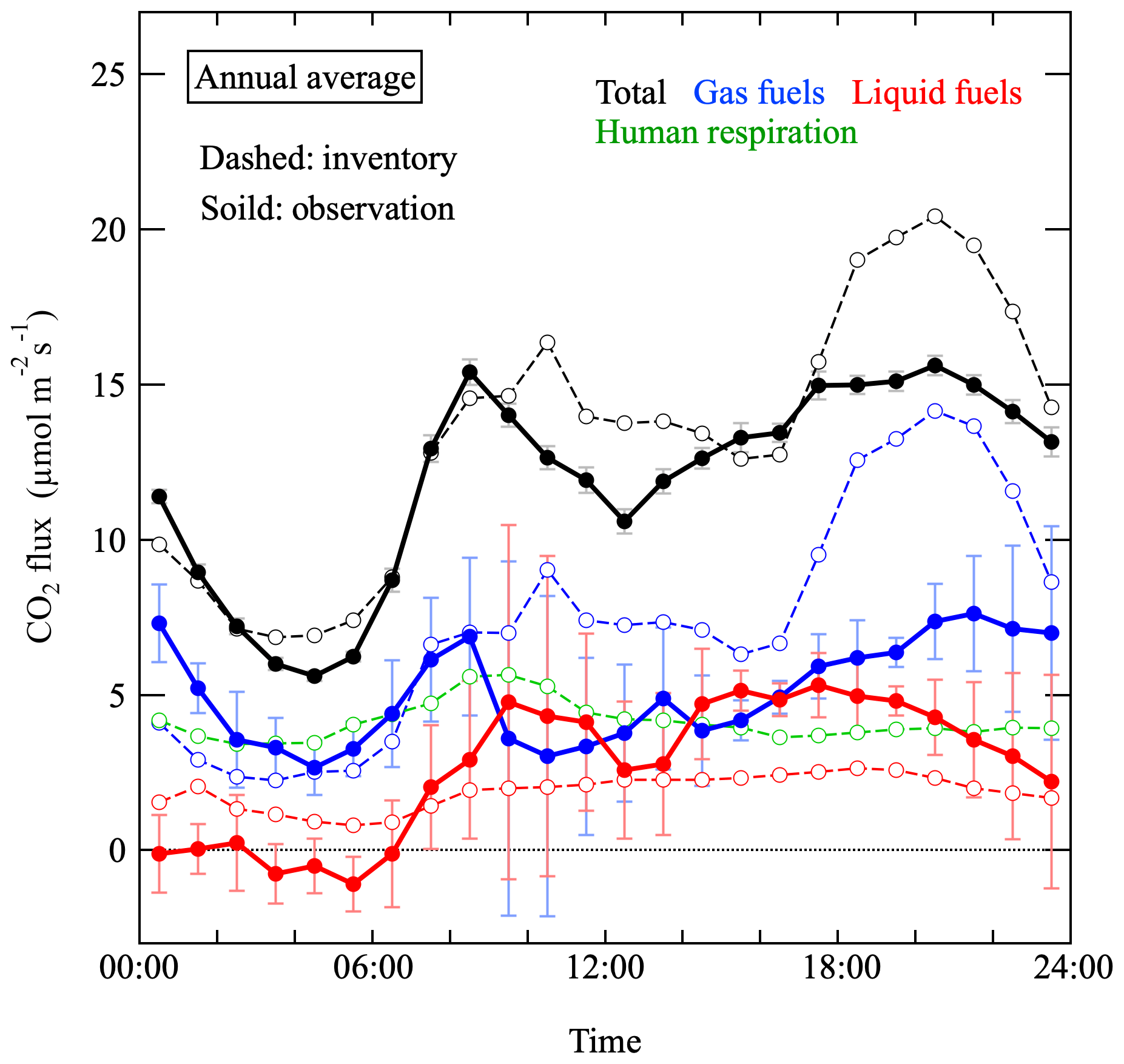
Figure 10Same as in Fig. 9 but for the annual average diurnal cycles. The error bars for the estimated CO₂ flux from liquid fuel consumption are the standard deviations of the diurnal cycles of the flux for respective seasons from the annual average cycle, assuming that the actual diurnal cycles of liquid fuel consumption do not change significantly throughout the year (see text).

Download