the Creative Commons Attribution 4.0 License.
the Creative Commons Attribution 4.0 License.
 | 14 Jan 2020
Mitigation of PM2.5 and ozone pollution in Delhi: a sensitivity study during the pre-monsoon period
Oliver Wild
Edmund Ryan
Saroj Kumar Sahu
Douglas Lowe
Scott Archer-Nicholls
Gordon McFiggans
Tabish Ansari
Vikas Singh
Ranjeet S. Sokhi
Alex Archibald
Gufran Beig
Fine particulate matter (PM2.5) and surface ozone (O3) are major air pollutants in megacities such as Delhi, but the design of suitable mitigation strategies is challenging. Some strategies for reducing PM2.5 may have the notable side effect of increasing O3. Here, we demonstrate a numerical framework for investigating the impacts of mitigation strategies on both PM2.5 and O3 in Delhi. We use Gaussian process emulation to generate a computationally efficient surrogate for a regional air quality model (WRF-Chem). This allows us to perform global sensitivity analysis to identify the major sources of air pollution and to generate emission-sector-based pollutant response surfaces to inform mitigation policy development. Based on more than 100 000 emulation runs during the pre-monsoon period (peak O3 season), our global sensitivity analysis shows that local traffic emissions from the Delhi city region and regional transport of pollution emitted from the National Capital Region (NCR) surrounding Delhi are dominant factors influencing PM2.5 and O3 in Delhi. They together govern the O3 peak and PM2.5 concentration during daytime. Regional transport contributes about 80% of the PM2.5 variation during the night. Reducing traffic emissions in Delhi alone (e.g. by 50 %) would reduce PM2.5 by 15 %–20 % but lead to a 20 %–25 % increase in O3. However, we show that reducing NCR regional emissions by 25 %–30 % at the same time would further reduce PM2.5 by 5 %–10 % in Delhi and avoid the O3 increase. This study provides scientific evidence to support the need for joint coordination of controls on local and regional scales to achieve effective reduction in PM2.5 whilst minimising the risk of O3 increase in Delhi.
- Article
(3094 KB) -
Supplement
(731 KB) - BibTeX
- EndNote


Exposure to air pollutants increases morbidity and mortality (J. Huang et al., 2018; WHO, 2013). The urban air quality in India, especially in Delhi, is currently among the poorest in the world (WHO, 2013, 2016a, b). In addition to the local impacts, the Indian monsoon can transport air pollutants to remote oceanic regions, inject them into the stratosphere and redistribute them globally (Lelieveld et al., 2018). This makes the impact of Indian air pollution wide-ranging regionally and globally, and it has interactions with climate and ecosystems worldwide (Menon et al., 2002; Gao et al., 2019).
PM2.5 (particulate matter with an aerodynamic diameter of less than 2.5 µm) is a major air pollutant, causing increases in disease (Pope et al., 2009; Gao et al., 2015; Stafoggia et al., 2019) and reduced visibility (Mukherjee and Toohey, 2016; Wang and Chen, 2019; Khare et al., 2018). The population of India experiences high PM2.5 exposure, and this is responsible for ∼1 million premature deaths per year (Conibear et al., 2018; Gao et al., 2018). Residential emissions are estimated to contribute ∼50 % of PM2.5 concentrations and to cause more than 0.5 million annual mortalities across India (Conibear et al., 2018). Previous studies reported an annual averaged PM2.5 loading of 110–140 µg m−3 in Delhi during 2015–2018, leading to ∼10 000 premature deaths per year in the city (Chen et al., 2019; Chowdhury and Dey, 2016; WHO, 2016a). In Delhi, the traffic sector (∼50 %) and the domestic sector (∼20 %) are the major local contributors to PM2.5 (Marrapu et al., 2014). Efforts to control traffic emissions in Delhi in recent years by introducing an alternating “odd–even” licence plate policy have led to reductions in PM2.5 of less than 10 % (Chowdhury et al., 2017). This indicates that there is an urgent need for a coordinated plan to mitigate PM2.5 pollution (Chowdhury et al., 2017).
Surface ozone (O3), another major air pollutant, is damaging to health and reduces crop yields (Ashworth et al., 2013; Lu et al., 2018; Kumar et al., 2018). The risks of respiratory and cardiovascular diseases are increased from short-term exposure to high ambient O3 and from long-term exposure at low levels (WHO, 2013; Turner et al., 2016; Fleming et al., 2018). Oxidation of volatile organic compounds (VOCs) in the presence of nitrogen oxides (NOx) is the main source of surface ozone. Rapid economic development in India has greatly increased the emissions of these O3 precursors (Duncan et al., 2016), leading to significant increases in O3 especially during the pre-monsoon period (Ghude et al., 2008). Hourly maximum O3 reaches as much as 140 ppbv during the pre-monsoon season in Delhi (Ghude et al., 2008), comparable to the most polluted regions in China (150 ppbv; Wang et al., 2017) and higher than the most polluted areas in the US (110 ppbv; Lu et al., 2018).
Mitigation of PM2.5 pollution may lead to an increase in surface ozone because the dimming effect of aerosols and removal of hydroperoxy radicals are reduced, facilitating O3 production (X. Huang et al., 2018; Li et al., 2018; Hollaway et al., 2019). Furthermore, co-reduction of NOx and PM2.5 emissions may increase O3 in cities where O3 production is in a VOC-limited photochemical regime (Ran et al., 2009; Xing et al., 2017, 2018). This has recently been reported in a number of Asian megacities, e.g. Shanghai (Silver et al., 2018), Beijing (Wu et al., 2015; Liu et al., 2017; Chen et al., 2018) and Guangzhou (Liu et al., 2013). Delhi and coastal cities in India, which are known to be VOC-limited (Sharma et al., 2017), may face increased O3 as a side effect of emission controls focused on PM2.5. Therefore, studies of mitigation strategies that target both PM2.5 and O3 are urgently needed (Chen et al., 2018), particularly as urban air pollution in India has been much less well studied than in many other countries.
To investigate the impacts of mitigation strategies with respect to both PM2.5 and O3, we demonstrate a framework for generating emission-sector-based pollutant response surfaces using Gaussian process emulation (O'Hagan and West, 2009; O'Hagan, 2006). The response surfaces describe how the pollutants, i.e. PM2.5 and O3, will respond to the changes in emissions from different sectors. We conduct global sensitivity analysis to identify the dominant emission sectors controlling PM2.5 and O3 and then generate sector-based response surfaces to quantify the impacts on PM2.5 and O3 of emission reductions. In contrast to simple sensitivity analysis varying one input at a time, this allows full exploration of the entire input space, accounting for the interactions between different inputs (Pisoni et al., 2018; Saltelli et al., 1999). Conventionally, chemical transport models (CTMs) are used to calculate the impacts on pollutants concentrations of different mitigation scenarios. However, the computational expense of CTMs makes them unsuitable for performing global sensitivity analysis or generating response surfaces, which usually require thousands of model runs. To overcome this difficulty, source–receptor relationships (Amann et al., 2011) or computationally efficient surrogate models, trained on a limited number of CTM simulations, are used to replace the expensive CTM. These approaches have been used to perform sensitivity and uncertainty analysis of regional air quality models (Pisoni et al., 2018), assessment of regional air quality plans (Zhao et al., 2017; Xing et al., 2017; Pisoni et al., 2017; Thunis et al., 2016), and sensitivity and uncertainty analysis of global and climate simulations (Ryan et al., 2018; Lee et al., 2012, 2016). Here, we use the surrogate model to explore the sensitivity of PM2.5 and O3 to sector-based emission controls in Delhi for developing a mitigation strategy addressing both pollutants.
In this study, we demonstrate the value of such a framework for supporting decision makers in determining better mitigation strategies. We give examples of its use in investigating impacts of mitigation scenarios on PM2.5 and O3 pollution in Delhi and demonstrate that regional joint coordination of emission controls over National Capital Region (NCR) of Delhi is essential for an effective reduction of PM2.5 whilst minimising the risk of O3 increase.

Figure 1Map of simulation domains, modified from © Google Earth.
2.1 WRF-Chem model baseline simulation
WRF-Chem (v3.9.1) – an online, fully coupled chemistry transport model (Grell et al., 2005) – has been widely used in previous studies of air quality across India (Marrapu et al., 2014; Mohan and Gupta, 2018; Gupta and Mohan, 2015; Mohan and Bhati, 2011). The model has also been used to estimate the health burden (Conibear et al., 2018; Ghude et al., 2016) and reduction in crop yields (Ghude et al., 2014) from the exposure to PM2.5 and O3 over India.
In this study, we focus on the hot and dry pre-monsoon period in Delhi, when average temperatures are around 32 ∘C and relative humidity (RH) is about 35 % (Ojha et al., 2012). O3 approaches its annual peak in the pre-monsoon period due to strong solar radiation (Ghude et al., 2008; Ojha et al., 2012). During the pre-monsoon period, desert dust can contribute significantly to particulate matter in Delhi (Kumar et al., 2014a, b). Here, we perform WRF-Chem simulation for the period of 2–15 May 2015 (with 2 additional days for spin-up), when Delhi was not significantly influenced by dust storms, according to MODIS observations (https://earthdata.nasa.gov/earth-observation-data/near-real-time/hazards-and-disasters/dust-storms, last access: 16 December 2019). Strong dust storms started to influence the Indo Gangetic Plain on 21–24 April and 19 May 2015, respectively. This minimises the uncertainties resulting from dust storm simulation and permits a stronger focus on anthropogenic emissions. Resuspended dust from road traffic is also a major contributor to PM2.5 in Delhi, and this is estimated and included in the emission inventory, as described below.
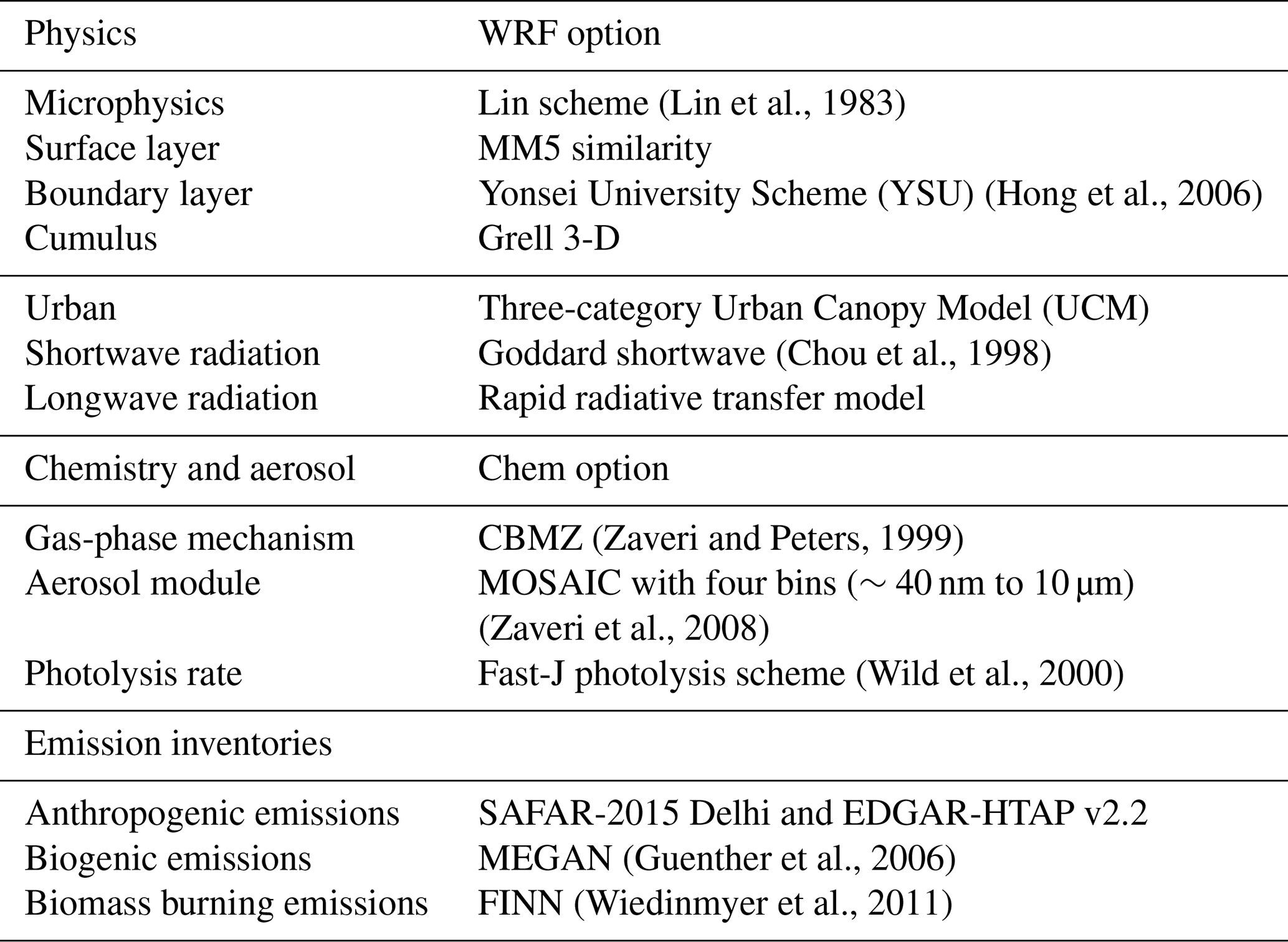
The model configuration follows the study of Marrapu et al. (2014), and the parameterisations used are listed in Table 1. Three nested domains are used, with coverage of southern Asia (45 km resolution), the Indo Gangetic Plain (15 km resolution), and the National Capital Region (5 km resolution; see Fig. 1). A test simulation with a fourth domain over Delhi at 1.67 km resolution suggests that a further increase in resolution does not substantially improve model performance (details in Sect. S1 in the Supplement), and this is in line with results from a previous study (Mohan and Bhati, 2011). The Carbon Bond Mechanism version Z (CBMZ; Zaveri and Peters, 1999) coupled with the MOSAIC (Zaveri et al., 2008) aerosol module with four size bins is used to represent gaseous chemical reaction and aerosol chemical and dynamical processes. We neglect wet scavenging and cloud chemistry processes here, as the impact of these is likely to be negligible during the dry pre-monsoon period over India. No precipitation was recoded in Delhi during the simulation period.
The initial and boundary conditions for chemical species are provided from MOZART-4 global results (https://www.acom.ucar.edu/wrf-chem/mozart.shtml, last access: 16 December 2019). Our baseline simulation is driven by the European Centre for Medium-Range Weather Forecasts (ECMWF) meteorological data, as we find that these reproduce regional meteorology better than those from the National Centers for Environmental Prediction (NCEP) over India, consistent with a recent study (Chatani and Sharma, 2018). The ECMWF reanalysis dataset (ERA-Interim) assimilates observations with a number of nearly 107 per day (Dee et al., 2011) and is used for grid nudging and as initial and boundary conditions for WRF-Chem at horizontal and temporal resolutions of 0.75∘ × 0.75∘ and 6 h, respectively. The wind pattern and temperature over Delhi in May 2015 are generally captured well in simulations driven by either meteorological dataset, but the model captures the variation in relative humidity much better (R=0.7) with ECMWF data than with NCEP data (R=0.4; negative bias of 20 %–40 %). A more detailed discussion is provided in Sect. S2.
The high-resolution Fire INventory from NCAR (FINN; Wiedinmyer et al., 2011) is adopted to provide biomass burning emissions. Interactive biogenic emissions are included using the Model of Emissions of Gases and Aerosols from Nature (MEGAN; Guenther et al., 2006). The global Emission Database for Global Atmospheric Research with Task Force on Hemispheric Transport of Air Pollution (EDGAR-HTAP; Janssens-Maenhout et al., 2015) version 2.2 (year 2010) at 0.1∘ × 0.1∘ resolution is used to represent anthropogenic emissions apart from over Delhi, where they are represented by a high-resolution monthly inventory for 2015 developed under the System of Air Quality and Weather Forecasting and Research (SAFAR) project (Sahu et al., 2011, 2015). In the absence of a diurnal variation in emissions specific to Delhi, we adopt diurnal variations from Europe in this study (Denier van der Gon et al., 2011). The SAFAR inventory provides emission fluxes of PM10, PM2.5, black carbon, organic carbon, NOx, CO, SO2 and NMVOCs (non-methane volatile organic compounds) from five sectors, including power (POW), industry (IND), domestic and residential (DOM), traffic (TRA), and wind-blown dust (WBD) from roads. Wind-blown dust includes dust resuspended from vehicle movement on paved and unpaved roads (Sahu et al., 2011) and is therefore closely related to traffic emissions, and we combine this into the traffic sector for our study.
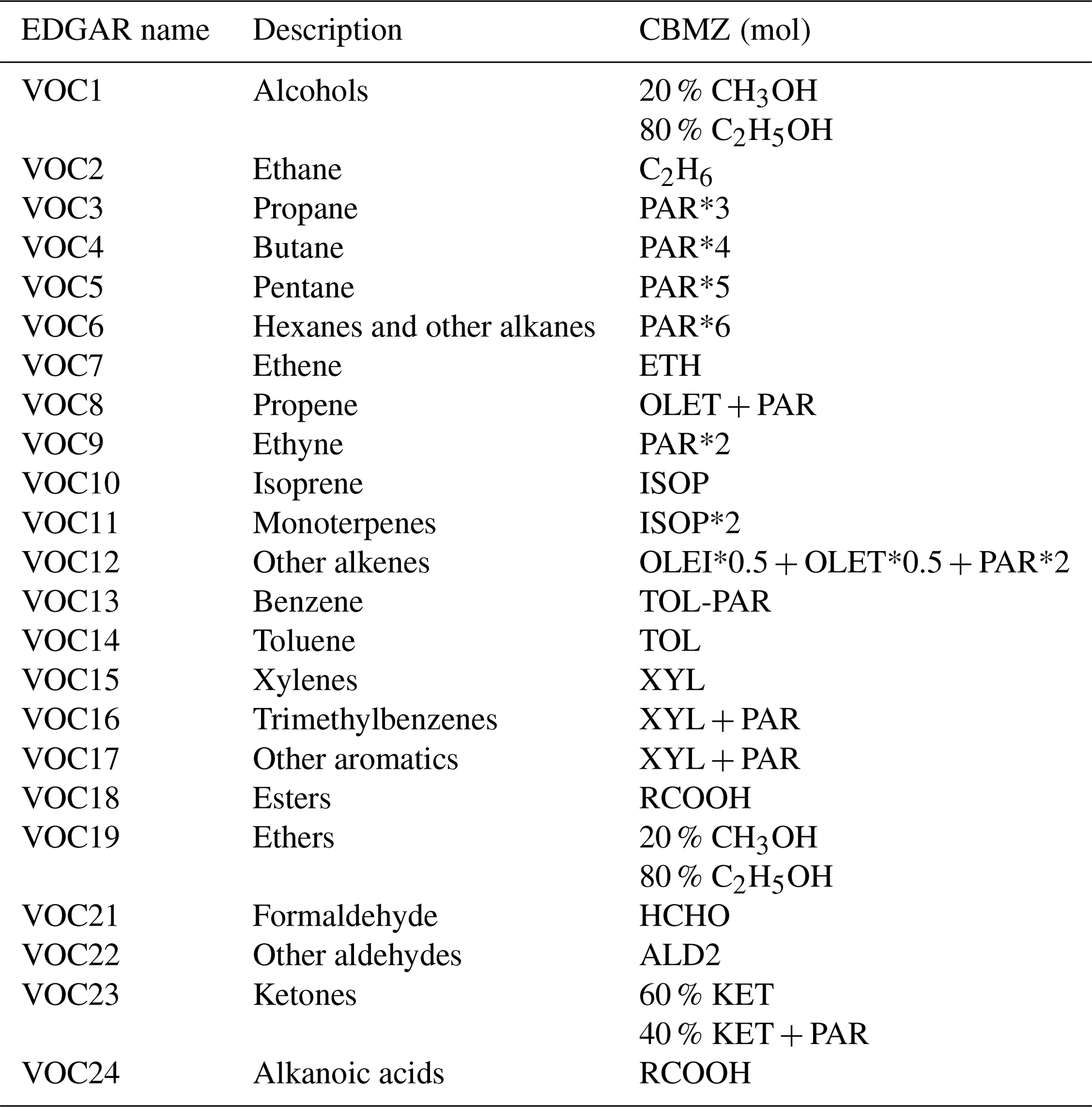
The NMVOC emissions are speciated according to the EDGAR (v4.3.2) global inventory (Huang et al., 2017) and are then lumped for the CBMZ chemistry scheme. The speciation mapping is detailed in Table 2 and described below, and a toolkit has been developed to perform this mapping. Emissions of alcohols and ethers are split 20 % : 80 % between methanol and ethanol by mass and then converted into molar emissions with a fractionation based on Murrells et al. (2009). Emissions of paraffin carbon (PAR) are calculated by converting mass emissions from each VOC group into molar emissions and then multiplying by the number of paraffin carbons in order to conserve carbon. Hexanes and higher alkanes are converted into molar emissions of hexane and then multiplied by 6 to give PAR emissions. Other alkenes are mapped to molar emissions of butane, and this is then apportioned between terminal olefin carbons (OLET), internal olefin carbons (OLEI) and PAR on a molar ratio of , following Zaveri and Peters (1999). Ketones are split 60 % : 40 % by mass between acetone (KET) and methyl-ethyl ketone (MEK) and then converted into molar emissions with fractions based on Murrells et al. (2009). As MEK is not included in the CBMZ mechanism, we apportion molar emissions of MEK equally between KET and PAR.
2.2 Observational network
Air quality and meteorological monitoring networks are operated in Delhi under the SAFAR project coordinated by IITM (Ministry of Earth Sciences, government of India). Measurements of PM2.5, O3 and NOx during the May 2015 simulation period are available from six monitoring stations in Delhi: Dr. CV Raman University (CVR), Delhi University (DEU), Indira Ghandi International Airport Terminal 3 (AIR), Aya Nagar (AYA), NCMRWF (NCM) and Pusa (PUS). The instruments are calibrated and measurements are quality controlled in the SAFAR project (http://safar.tropmet.res.in, last access: 16 December 2019); more details are given in previous studies (Sahu et al., 2011; Beig et al., 2013; Aslam et al., 2017). Site locations are shown in Fig. 2, and measured variables are given in Table S1 in the Supplement.
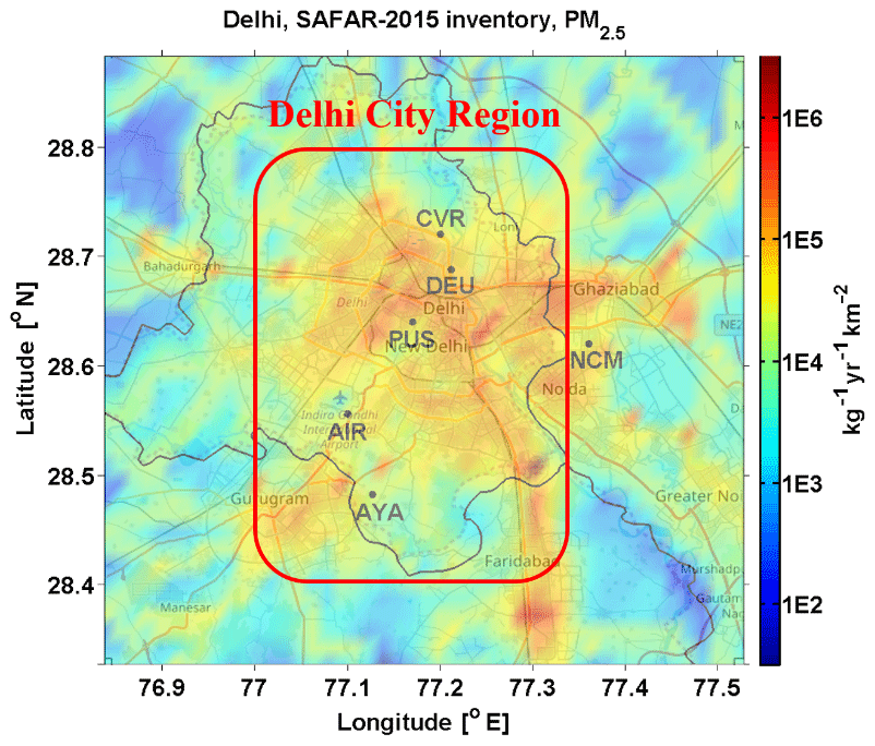
Figure 2SAFAR inventory of total PM2.5 emissions. The locations of measurement sites over Delhi are marked by black dots, and the Delhi city region is marked by a red box. This figure is modified from OpenSteetMap. © OpenStreetMap contributors 2019. Distributed under a Creative Commons BY-SA License.
2.3 Global sensitivity analysis of urban air pollution
We perform global sensitivity analysis (GSA; Iooss and Lemaître, 2015) to quantify the sensitivity of modelled outputs (PM2.5 and O3 for this study) to changes in the model inputs, which for this study are emissions from the different emission sectors. One-at-a-time sensitivity analysis is a common way of calculating model sensitivity and involves varying a single model input while the other inputs are fixed at nominal values, e.g. Wild (2007). While one-at-a-time approach is relatively easy to implement, it assumes that the model response to different inputs is independent, and this can lead to biased results (Saltelli et al., 1999; Pisoni et al., 2018; Carslaw et al., 2013). GSA overcomes the problems of the one-at-a-time approach by averaging over the other inputs rather than fixing them at specific values. This allows calculation of first-order sensitivity indices (SIs) for each variable, corresponding to the ith input variable and the jth output point, given by Eq. (1) (Ryan et al., 2018):
where xi is the ith element of the input, and yj is the jth element of the output. “E(⋅)” and “Var(⋅)” denote the mathematical functions that calculate the expectation and variance, respectively. The simplest way of computing SIi,j is by brute force, but this is also the most computationally intensive (Ryan et al., 2018).
The extended Fourier amplitude sensitivity test (eFAST), first developed by Saltelli et al. (1999), is a commonly used approach to perform GSA and calculate SIs and is adopted in this study because of its high efficiency. A basic overview and detailed equations of the eFAST method are given in the Sect. 2.2.2 of Ryan et al. (2018). A challenge of using eFAST is that it typically requires thousands of model runs. To overcome this, we employ a computationally cheaper surrogate model in place of our expensive simulation model WRF-Chem. A surrogate model is a simple model (usually statistical) which can map the inputs to the outputs of the simulation model with sufficiently good accuracy, given the same inputs. In this study, we choose a type of surrogate model called a Gaussian process emulator, which works like a function for multidimensional interpolation and has been used extensively in many areas of applied science (Carslaw et al., 2013; Koehler and Owen, 1996; Queipo et al., 2005; Vanuytrecht and Willems, 2014; Vu et al., 2015; Degroote et al., 2012) and uncertainty assessments of atmospheric models (Lee et al., 2011, 2012, 2016). Gaussian process emulators typically require a relatively small number of runs of the computationally expensive model to generate; this is in contrast to other surrogate modelling approaches, such as neural networks, which typically require thousands of model runs to train them. For a basic overview of a Gaussian process emulator, see O'Hagan (2006); a detailed introduction and equations are also given in the Sect. 2.3 of Ryan et al. (2018). Before using the emulator in place of the WRF-Chem model to carry out the thousands of model runs required for GSA, we train the emulator using a relatively small number of WRF-Chem model runs. Following previous studies (Carslaw et al., 2013; Lee et al., 2016), a maximin Latin hypercube space-filling design is employed to select the designs of training runs for WRF-Chem. Latin hypercube sampling is a statistical method for generating a near-random sample of parameter values from a multidimensional distribution (Shields and Zhang, 2016). Here, we search through 100 000 Latin hypercube random designs to find the optimal one, where the parameter space is filled most effectively. This ensures that the sets of inputs chosen cover as large a fraction of the input space as possible. Full details (including R codes) of how to generate the Gaussian process emulator, eFAST method and GSA can be found in Ryan et al. (2018).
In this study, we focus on a limited number of the emission sectors to demonstrate the effectiveness of the approach: domestic or residential emissions in Delhi (DOM), traffic emissions in Delhi (TRA, including WBD), power and industry in Delhi (POW + IND), and total emissions in the NCR outside Delhi. NCR represents the contribution of regional transport to pollution in Delhi. According to the SAFAR emission inventory, the total PM2.5 emissions of DOM, TRA, POW+IND and NCR are about 1.8, 6.1, 3.1 and 8.5 Gg per month in May 2015, respectively. The Gaussian process emulator is trained using 20 executions of the WRF-Chem model, with emission scaling drawn from a variation range of 0 %–200 % for each of the four specified sectors (Table S2). Emulation of the impacts of mitigation scenarios on PM2.5 and O3 can be performed in minutes on a laptop, in contrast to simulations with WRF-Chem, which require a few days on a high-performance computing cluster. The accuracy of the emulator as a surrogate of the WRF-Chem model is evaluated using a “leave-one-out” cross validation (Bastos and O'Hagan, 2009). This involves training the emulator using 19 out of the 20 sets of inputs and outputs from the WRF-Chem model runs and then evaluating the emulator against the 20th simulation. This process is carried out for each of the 20 sets of inputs and outputs. Given that the output space is multidimensional (i.e. modelled O3 and PM2.5 varied spatially and in time), the emulator is validated by comparing 10 000 (random samples varied spatially and in time) emulator output values against the corresponding output values of the WRF-Chem model. The emulator validation plot is shown in Fig. 3. Modelled and emulated O3 and PM2.5 lie very close to the 1:1 line with R2 values of more than 95 %, as shown in Fig. 3, indicating that the emulation provides an accurate representation of the input–output relationship of the WRF-Chem model.
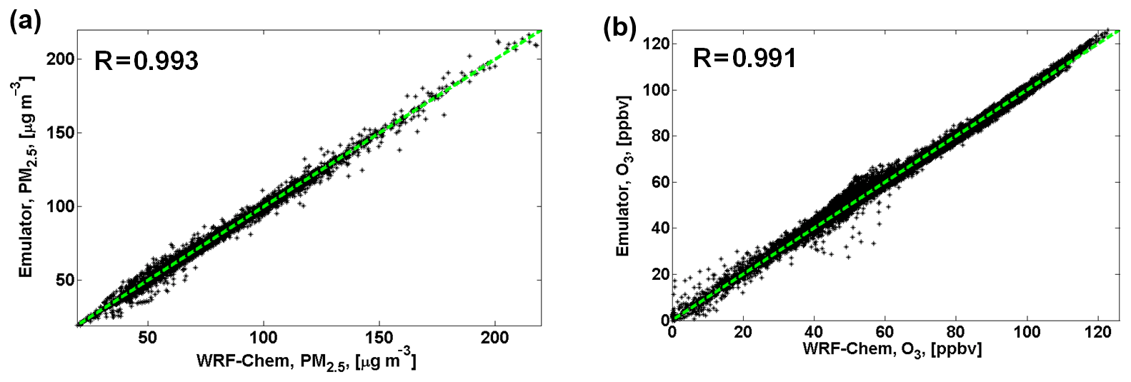
Figure 3Validation of Gaussian process emulator with WRF-Chem model. (a) PM2.5; (b) O3. The green dashed line indicates the 1:1 line.
2.4 Response surfaces
Response surfaces are useful for investigating the relationship between model inputs and outputs, in this case between sectoral emissions and modelled pollutant concentrations. They have been widely applied for air quality studies and policymaking (EPA, 2006a, b, Zhao et al., 2017; Xing et al., 2017). Here, we analyse the responses of PM2.5 and O3 to changes in emissions from each sector of between 0 % and 200 %. The computationally efficient Gaussian process emulation enables us to generate response surfaces without the computational burden of a large number of runs of the WRF-chem model.
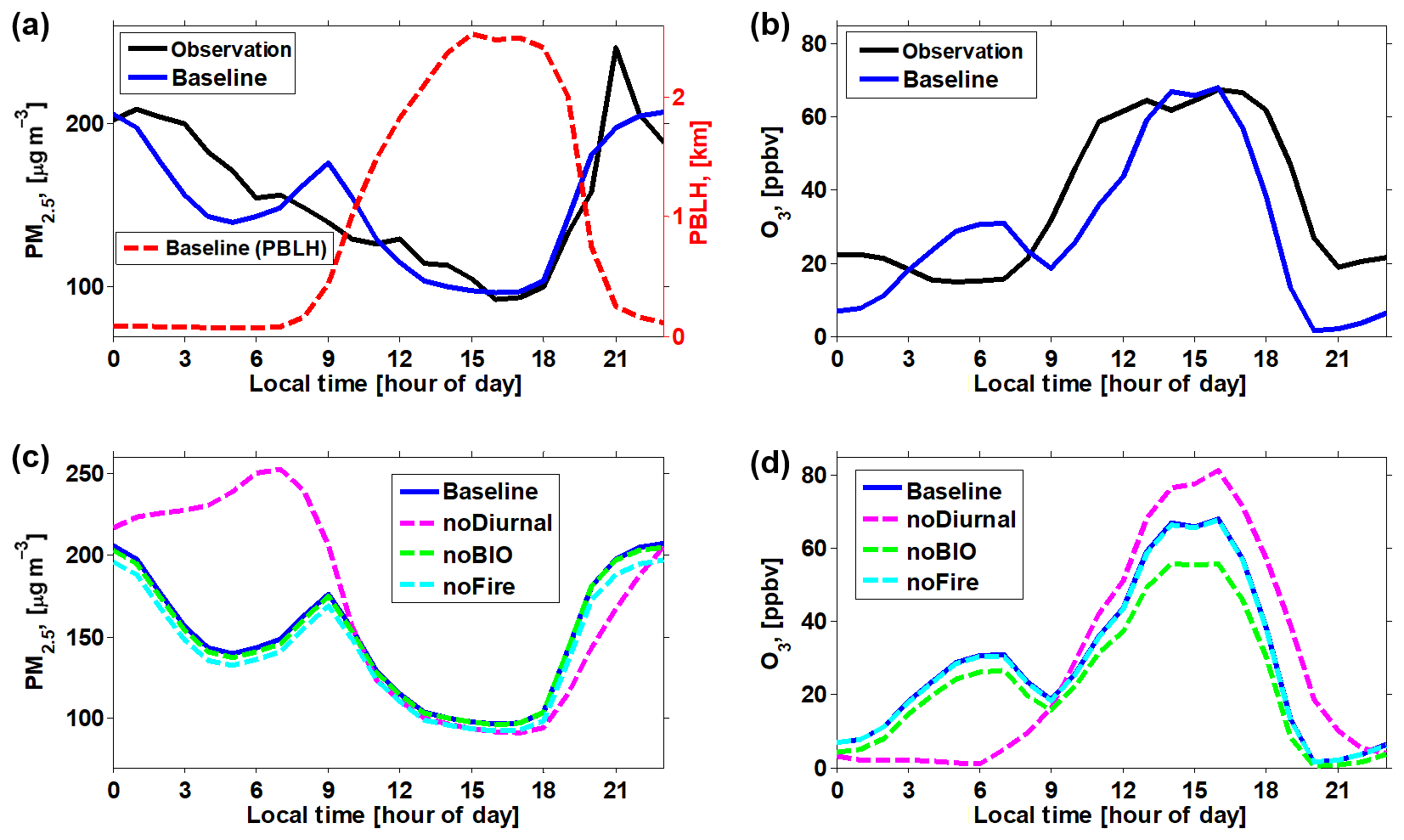
Figure 4Average diurnal patterns of pollutants during the 2–15 May 2015 simulation period. (a) Modelled and observed PM2.5 and model PBL height (PBLH), (b) O3, (c) results of sensitivity studies for PM2.5, and (d) results of sensitivity studies for O3. (a) and (c) are for site CVR, and (b) and (d) are for site AIR (marked in Fig. 2). The sensitivity runs “noFire” and “noBIO” show model results without biomass burning and biogenic emissions, respectively, and “noDiurnal” shows model results with constant anthropogenic emissions rates throughout the day.
2.5 Outline of analysis
We use the WRF-Chem model to simulate the hourly concentrations of O3 and PM2.5 over the Delhi region during 2–15 May 2015 and evaluate the results against observations. We perform a simple sensitivity analysis to investigate the contributions of biomass burning and biogenic emissions to PM2.5 and O3 in Delhi. We then conduct a global sensitivity analysis, using the eFAST method (see Sect. 2.3) along with Gaussian process emulation to determine the sensitivity of modelled O3 and PM2.5 concentrations to changes in the dominant anthropogenic emission sectors. Finally, we generate response surfaces to identify appropriate mitigation strategies for reducing PM2.5 while minimising the risks from O3 increase.
3.1 Model performance
The WRF-Chem model captures the general magnitude and variation in PM2.5 well (Fig. 4a), with a mean bias and error of about −3.5 % and 11 %, respectively and an index of agreement (Willmott et al., 2012) of 75 %. The frequency distributions of modelled PM2.5 are also similar to the observations, with differences in mean and median concentrations of less than 10 %, although high concentration spikes are missed by the model (Fig. S1 in the Supplement). The modelled PM2.5 peaks at around 09:00 LT (local time) because the rush hour enhances traffic emissions before the planetary boundary layer (PBL) height has increased (Fig. 4a). This is also seen in the modelled results at DEU (Fig. S2), which is closer to a motorway and shows a more intense PM2.5 peak in the morning rush hour. PM2.5 is overestimated during the morning rush hour (around 09:00 LT) and underestimated during the early morning (03:00–05:00 LT; Figs. 4a and S2). This may suggest that there is an earlier rush hour or more traffic activity at night in Delhi than in European cities, since we adopted European diurnal emission patterns in this study in the absence of local information. Detailed studies of traffic emissions and their variation in Delhi would help improve these model simulations.
The modelled chemical composition of PM2.5 is shown in Fig. S3. Secondary inorganic aerosol (SIA), including sulfate, nitrate and ammonium, only contributes ∼25 % of aerosol mass in our simulation. In the absence of particle inorganic composition measurements during the simulation period, we compare our results with a previous modelling study of Delhi during the post-monsoon season (Marrapu et al., 2014), which also shows a ∼25 % contribution of SIA to PM2.5 loading, in line with our results. Furthermore, our results are also consistent with an observational study, which reported the mass fraction of organic matter (usually calculated as 1.4 times organic carbon, OC) and elemental carbon (usually equivalent to black carbon in modelling studies; Chen et al., 2016b) in PM2.5 of ∼20 % and ∼6 % in Delhi during May 2015, respectively (Sharma et al., 2018).
The model captures the peak O3 well, with a bias of less than 5 %, although it underestimates O3 during night-time (Fig. 4b). In general, the diurnal pattern and magnitude of O3 are captured by WRF-Chem (Fig. 4b), with a normalised mean bias and error of about −20 % and 35 %, respectively, and an index of agreement of 65 %. The underestimation during night-time is likely to be because NOx is overestimated by a factor of 2–3 at night (Fig. S4), and the excess NO depletes O3. This is indicated by the frequency distribution of O3 and NOx (Fig. S5), where the median values of observed O3 and NOx are matched well by the model. However, the higher peaks of modelled NOx concentration lower the modelled O3 levels, indicating that Delhi is in the VOC-limited photochemical regime. Similar results are found at AYA (Fig. S6). The larger underestimation of O3 at NCM (Fig. S5d; industrial environment site) suggests that NOx emission from the industry sector may be overestimated.
3.2 Impacts of biogenic and biomass burning emissions
Before exploring the importance of the four selected anthropogenic emission sectors on PM2.5 and O3 in Delhi during the simulation period, we investigate the contributions from other factors (biomass burning and biogenic emissions). We turn off these sources in the WRF-Chem simulation and find that there is a negligible contribution from biogenic emissions to PM2.5 concentrations over Delhi in this season (Fig. 4c and d). It is worth noting that biogenic emissions may contribute to secondary organic aerosol (SOA) in Delhi, but the formation of SOA is not represented well by the CBMZ–MOSAIC chemistry–aerosol mechanisms used in this study. However, this weakness is not expected to have a major influence on our pre-monsoon results; as described above, the difference of organic matter fraction between simulation and observation (Sharma et al., 2018) in May 2015 is less than 5%. About 10% of PM2.5 in Delhi is derived from biomass burning during the simulation period. Crop burning in Haryana and Punjab states is a major source of this (Jethva et al., 2018; Cusworth et al., 2018). In contrast, there is a negligible contribution from biomass burning to O3. However, there is a 15 %–20 % contribution to O3 from biogenic emission of VOCs, highlighting the fact that O3 production in Delhi is strongly VOC-limited.
3.3 Effect of the diurnal variation in emissions
In order to investigate the competing influences of meteorology and human activities on the diurnal patterns of PM2.5 and O3 over Delhi, we test the effect of removing the diurnal variation in anthropogenic emissions (“noDiurnal”; see Fig. 4c and d). Modelled PM2.5 concentrations are very similar to the “baseline” run during daytime, when the PBL is well developed, with differences of less than 5 %. This suggests that meteorological processes such as vertical mixing, advection and transport are the dominant factors controlling PM2.5 in the daytime. In contrast, freshly emitted pollutants are trapped at night when the PBL is shallow, and concentrations are very sensitive to the emission flux so that the diurnal pattern of emissions is the dominant factor at night. The PM2.5 concentration is almost doubled in the early morning (03:00–09:00 LT; Fig. 4c), when the PBL is shallow and emissions in the noDiurnal case are higher. There is also a large increase in NOx in the early morning (Fig. S4), which leads to greater depletion of O3 (Fig. 4d). However, the concentration of O3 is about 20 %–25 % higher during the ozone peak hour in the afternoon in the noDiurnal case, as the daytime NOx emissions are less (Fig. S4). This sensitivity test also highlights the VOC-limited nature of O3 production in Delhi.
3.4 Sensitivity analysis of pollutants in Delhi
The importance of each anthropogenic emission sector to pollutant concentrations in Delhi is investigated using global sensitivity analysis and indicated by global sensitivity indices (SIs), as shown in Fig. 5. The sensitivity index is a measure of the contribution of the variation in pollutants from one emission sector to the total variation across all four sectors considered here. A larger SI indicates a larger influence from the corresponding sector to the modelled average surface PM2.5 or O3 over the Delhi city region (marked in Fig. 2) in this study.
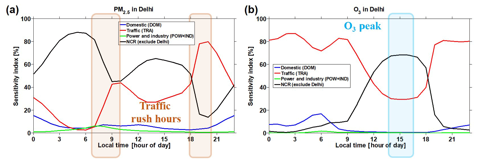
Figure 5Averaged diurnal pattern of global sensitivity indices during the 2–15 May simulation period. (a) PM2.5; (b) O3. The PM2.5 and O3 results are averaged over Delhi city region (marked with red box in Fig. 2). The morning and evening rush hours and the period of peak ozone are marked with the boxes to highlight the notable changes in contribution from each emission sector.
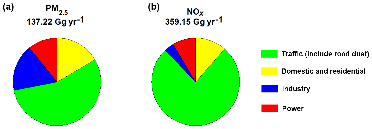
Figure 6Annual emission of different sectors in Delhi from SAFAR inventory. (a) PM2.5; (b) NOx. The emissions of black carbon, organic carbon, non-methane VOC (NMVOC) and SO2 are given in Fig. S13.
The PM2.5 concentration is most sensitive to emissions from the NCR region surrounding Delhi, with a sensitivity index higher than 50 % most of time (Fig. 5a) and reaching 80 %–90 % and ∼60 % during 03:00–07:00 LT and 12:00–17:00 LT, respectively. During the rush hours in the morning and evening, the sensitivity to NCR emissions is lower, while the sensitivity to Delhi traffic emissions increases by ∼30 %. Around 10:00 LT, local traffic emissions and emissions from NCR have a similar effect on PM2.5. In contrast, local traffic emissions dominate the PM2.5 in Delhi around 20:00 LT, with a sensitivity contribution of up to ∼80 %. This is caused by the collapse of the PBL in the evening rush hour at around 20:00 LT, which enhances the sensitivity to fresh local emissions. Local traffic emissions contribute ∼60 % of primary PM2.5 emission in Delhi (Fig. 6a), which remains concentrated in the PBL during rush hours. In contrast, the fully developed PBL in the daytime mixes air down from the free troposphere (Chen et al., 2016a), where regional transport of pollutants from NCR can be important. This could explain the second peak in the sensitivity to NCR emissions (50 %–60 %) during the afternoon (Fig. 5a).
The variation in O3 in the Delhi city region is overwhelmingly dominated by local traffic emissions, with a sensitivity index higher than 80 % at night-time (Fig. 5b), when O3 and traffic emissions are anti-correlated. Traffic contributes ∼75 % of total NOx emission in Delhi (Fig. 6b), and the shallow PBL during the night traps the NOx. This removes O3 through chemical reaction in the absence of solar radiation. As the PBL develops in the morning, the sensitivity of O3 to traffic decreases and the sensitivity to NCR emissions increases. The sensitivity to NCR emissions reaches its highest point (70 %) when the PBL is fully developed at around 15:00 LT. As discussed above, the downward mixing of air from the free troposphere and dilution of local emissions in the fully developed PBL could be the reason for this. The O3 peak coincides with the highest PBL at this time because photolysis and development of the PBL are both driven by solar radiation. The development of the PBL increases the contribution from regional transport, and precursors emitted from the NCR are one of the dominant contributors to the peak of O3 in Delhi. NOx, mainly originating from traffic emissions, is underestimated by ∼30 % during the O3 peak period (Fig. S4). This uncertainty can propagate into the Gaussian process emulator and could lead to underestimation of the influence of traffic on peak O3 but is not expected to change the nature of our conclusion about the predominance of regional transport and local traffic emissions. In addition, it is noteworthy that the NOx-rich urban plume from Delhi has a substantial influence on O3 in downwind regions across the NCR as well, as discussed in Sect. S3.
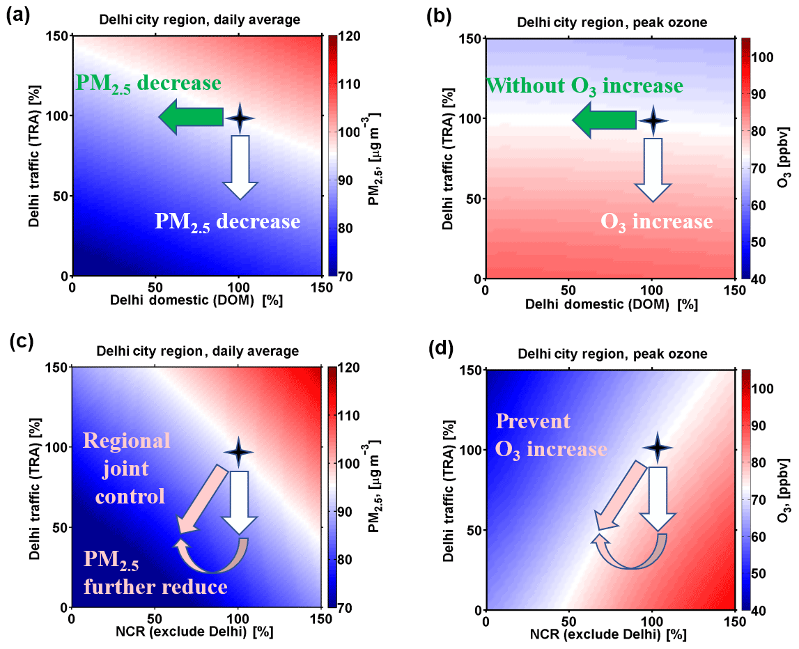
Figure 7Response surfaces for PM2.5 and ozone concentrations over Delhi city region, averaged over 2–15 May 2018. (a) Daily average of PM2.5 concentrations as a function of local traffic and domestic emissions in Delhi, (b) peak hourly ozone concentrations as a function of local traffic and domestic emissions in Delhi, (c) daily average of PM2.5 concentrations as a function of local traffic emissions in Delhi and emissions in NCR region surrounding Delhi, and (d) peak hourly ozone concentrations as a function of local traffic emissions in Delhi and emissions in NCR region surrounding Delhi. The star indicates current conditions, and the arrows show the effect of possible emission controls.
3.5 Mitigation strategies
To demonstrate a framework for developing better mitigation strategies for addressing both PM2.5 and O3 pollution in Delhi, emission-sector-based pollutant response surfaces are generated using Gaussian process emulation (Fig. 7). For local emissions in Delhi, we focus mainly on traffic and residential sectors here because we find that power and industrial emissions have a more limited influence on PM2.5 and O3 concentrations in Delhi (Fig. 5). A range of different mitigation strategies are analysed, aiming at mitigating PM2.5 pollution whilst minimising the risk of O3 increase.
We find that the responses of PM2.5 and O3 to each emission sector are nearly linear in Delhi. The response surfaces show that reducing local traffic emissions in Delhi leads to an efficient decrease in PM2.5 loading (Fig. 7a) but increases O3 greatly (Fig. 7b). Reducing local domestic emissions decreases PM2.5 loading less than reducing traffic but without increasing O3. The small impact on O3 may be because domestic emissions are not a major source of NOx, contributing only 15 % of that from traffic (Fig. 6). A 10 %–20 % reduction in NOx is expected when reducing local domestic emissions by 50 %; however a 35 %–45 % reduction is seen for a 50 % reduction in local traffic emissions (Fig. S7). In addition, VOC is reduced more than NOx when controlling domestic emissions, as the VOC ∕ NOx emission ratio (kg kg−1) is 1.8 in contrast to a ratio of 0.4 for traffic emissions. Greater reduction of VOC suppresses the increase in O3 in Delhi, which is a VOC-limited environment. A reduction in local traffic emissions alone of 50 % could decrease Delhi PM2.5 loading by 15 %–20 %, but this would also increase O3 by 20 %–25 %. We note that our model may underestimate the influence of traffic emissions on O3 to some extent, as described above (Sect. 3.4), suggesting that the ozone increase could be stronger than we predict. To prevent the side effect of increasing O3 by controls on traffic emissions, regional cooperation would be required to reduce emissions in the NCR region surrounding Delhi by 25 %–30 %, which also permits a further reduction of PM2.5 by 5 %–10 % (Fig. 7c and d). This is consistent with a recent study showing that ∼60 % of PM2.5 in Delhi originates from outside (Amann et al., 2017). We test this by performing an additional run with WRF-Chem, using emission reductions of 50 % and 30 % for sectors of local traffic and the surrounding NCR region, respectively. We compare the WRF-Chem results of the additional run and the base case (without change of emissions) against the corresponding results from Gaussian process emulator (Fig. S8). We find that the PM2.5 and O3 results from the model runs lie within 5 % of those estimated with the emulator and with R2 higher than 95 %, demonstrating the high quality of the emulation approach adopted here and underlining its deeper value for identifying mitigation approaches. The suggested regional joint mitigation with NCR surrounding Delhi is in line with a recent study for mitigating PM2.5 in Beijing, which showed that regional coordination over the North China Plain could lead to a reduction in PM2.5 of up to 40 % in winter (Liu et al., 2016).
Previous studies have shown that emission controls focusing on mitigation of PM2.5 may result in substantial increases in surface ozone over urban areas that are in a VOC-limited photochemical environment. Comprehensive studies of mitigation strategies with respect to both PM2.5 and O3 are urgently required but are limited in India. In this study, we demonstrate a numerical framework for informing emission-sector-based mitigation strategies in Delhi that account for multiple pollutants.
By using Gaussian process emulation with an air quality model (WRF-Chem), we generate a computationally efficient surrogate model for performing global sensitivity analysis and calculating emission-sector-based pollutant response surfaces. These enable us to exhaustively investigate the impacts of different mitigation scenarios on PM2.5 and O3 in Delhi, which help decision makers choose better mitigation strategies. Global sensitivity analysis shows that pollutants originating from the National Capital Region (NCR) surrounding Delhi and local traffic emissions are the major contributors of PM2.5 and O3 in Delhi. They co-dominate the O3 peak and PM2.5 in Delhi during daytime, while the regional transport governs PM2.5 during the night, in line with a recent study showing that ∼60 % of PM2.5 in Delhi originates from outside (Amann et al., 2017). Controlling local traffic emissions in Delhi would have the notable side effect of increasing O3, at least in the pre-monsoon and summer period (peak O3 season) that we consider here. This is in line with recent increases in O3 seen in China (Silver et al., 2018; Li et al., 2018). The Chinese experience suggests that regional joint coordination is required to effectively mitigate PM2.5 pollution in Beijing (Liu et al., 2016). Our pollutant response surfaces go one step further and suggest that joint coordinated emission controls with the NCR region surrounding Delhi would be required to not only achieve a more ambitious reduction of PM2.5 but also to minimise the risk of O3 increases. In the regional joint coordination, residential energy use could be a dominant emission sector over a large region in India (Conibear et al., 2018).
The experiences of developed countries (Dooley, 2002; EPA, 2011) and recently in China (J. Huang et al., 2018; Wang et al., 2019) show that regional joint coordination can be achieved by changing energy infrastructure (e.g. replacing fossil fuel by renewable energy and natural gas), desulfurisation and denitrification technologies, popularisation of new energy vehicles, strict control of vehicle exhaust, and reducing road and construction dust. Further studies with more detailed information on specific emission sectors and strategies for clean-technology development and popularisation would permit deeper insight into air pollution mitigation approaches suitable for Delhi. These are needed to address both PM2.5, which has a higher impact on public health (e.g. J. Huang et al., 2018), and O3, which greatly impacts regional ecology and agriculture (e.g. Avnery et al., 2011). A more comprehensive evaluation of the health and economic benefits of different mitigation strategies would greatly help Indian decision makers, and the framework we have demonstrated here would provide a strong foundation for this.
NCEP FNL operational model global tropospheric analyses (ds083.2) were downloaded from https://rda.ucar.edu/data/ds083.2/ (NCEP/National Weather Service/NOAA/U.S. Department of Commerce, 2000), and sea surface temperature data were downloaded from https://polar.ncep.noaa.gov/sst/ (NCEP SST, 2019). ECMWF interim reanalyses (ERA-Interim) were downloaded from http://apps.ecmwf.int/datasets/data/interim-full-daily (ECMWF, 2019). MOZART-4 global model results were downloaded from https://www.acom.ucar.edu/wrf-chem/mozart.shtml (NCAR, 2019). The FINN biomass burning emissions dataset was downloaded from http://bai.acom.ucar.edu/Data/fire/ (Wiedinmyer et al., 2011). Toolkits for emission processing are available from https://github.com/douglowe/WRF_UoM_EMIT/releases/tag/v1.0 (Lowe, 2019a) and https://github.com/douglowe/PROMOTE-emissions/releases/tag/v1.0 (Lowe, 2019b).
The supplement related to this article is available online at: https://doi.org/10.5194/acp-20-499-2020-supplement.
OW and YC conceived the study. YC performed the simulations and emulation and processed and interpreted the results, with help from YW. ER designed and built the Gaussian process emulator. GB and SKS provided the observations and SAFAR emission inventory. DL, AA, SAN and GM helped with pre-processing the emission data and developing the emission toolkit. VS and RSS provided useful discussion on the emission inventory. RSS led the development of the PROMOTE project. YC and OW wrote the paper, with input from all co-authors.
The authors declare that they have no conflict of interest.
The Indian Institute of Tropical Meteorology, Pune, is supported by the Ministry of Earth Science, government of India. The observations and high-resolution emission inventory are provided by the SAFAR project under MoES (http://safar.tropmet.res.in, last access: 16 December 2019). The authors appreciate the efforts of the entire team involved in the PROMOTE and SAFAR projects. The paper is based on interpretation of scientific results and in no way reflects the viewpoint of the funding agency.
This research has been supported by the Natural Environment Research Council (NERC) of the UK (grant nos. NE/P016405/1, NE/N003411/1 and NE/P016480/1).
This paper was edited by Frank Dentener and reviewed by two anonymous referees.
Amann, M., Bertok, I., Borken-Kleefeld, J., Cofala, J., Heyes, C., Höglund-Isaksson, L., Klimont, Z., Nguyen, B., Posch, M., Rafaj, P., Sandler, R., Schöpp, W., Wagner, F., and Winiwarter, W.: Cost-effective control of air quality and greenhouse gases in Europe: Modeling and policy applications, Environ. Model. Softw., 26, 1489–1501, https://doi.org/10.1016/j.envsoft.2011.07.012, 2011.
Amann, M., Purohit, P., Bhanarkar, A. D., Bertok, I., Borken-Kleefeld, J., Cofala, J., Heyes, C., Kiesewetter, G., Klimont, Z., Liu, J., Majumdar, D., Nguyen, B., Rafaj, P., Rao, P. S., Sander, R., Schöpp, W., Srivastava, A., and Vardhan, B. H.: Managing future air quality in megacities: A case study for Delhi, Atmos. Environ., 161, 99–111, https://doi.org/10.1016/j.atmosenv.2017.04.041, 2017.
Ashworth, K., Wild, O., and Hewitt, C. N.: Impacts of biofuel cultivation on mortality and crop yields, Nat. Clim. Change, 3, 492–496, https://doi.org/10.1038/nclimate1788, 2013.
Aslam, M. Y., Krishna, K. R., Beig, G., Tinmaker, M. I. R., and Chate, D. M.: Seasonal Variation of Urban Heat Island and Its Impact on Air-Quality Using SAFAR Observations at Delhi, India, Am. J. Clim. Change, 6, 294–305, https://doi.org/10.4236/ajcc.2017.62015, 2017.
Avnery, S., Mauzerall, D. L., Liu, J., and Horowitz, L. W.: Global crop yield reductions due to surface ozone exposure: 2. Year 2030 potential crop production losses and economic damage under two scenarios of O3 pollution, Atmos. Environ., 45, 2297–2309, https://doi.org/10.1016/j.atmosenv.2011.01.002, 2011.
Bastos, L. S. and O'Hagan, A.: Diagnostics for Gaussian Process Emulators, Technometrics, 51, 425–438, https://doi.org/10.1198/TECH.2009.08019, 2009.
Beig, G., Chate, D. M., Ghude, S. D., Ali, K., Satpute, T., Sahu, S. K., Parkhi, N., and Trimbake, H. K.: Evaluating population exposure to environmental pollutants during Deepavali fireworks displays using air quality measurements of the SAFAR network, Chemosphere, 92, 116–124, https://doi.org/10.1016/j.chemosphere.2013.02.043, 2013.
Carslaw, K. S., Lee, L. A., Reddington, C. L., Pringle, K. J., Rap, A., Forster, P. M., Mann, G. W., Spracklen, D. V., Woodhouse, M. T., Regayre, L. A., and Pierce, J. R.: Large contribution of natural aerosols to uncertainty in indirect forcing, Nature, 503, 67–71, https://doi.org/10.1038/nature12674, 2013.
Chatani, S. and Sharma, S.: Uncertainties Caused by Major Meteorological Analysis Data Sets in Simulating Air Quality Over India, J. Geophys. Res.-Atmos., 123, 6230–6247, https://doi.org/10.1029/2017JD027502, 2018.
Chen, L., Guo, B., Huang, J., He, J., Wang, H., Zhang, S., and Chen, S. X.: Assessing air-quality in Beijing-Tianjin-Hebei region: The method and mixed tales of PM2.5 and O3, Atmos. Environ., 193, 290–301, https://doi.org/10.1016/j.atmosenv.2018.08.047, 2018.
Chen, Y., Cheng, Y., Ma, N., Wolke, R., Nordmann, S., Schüttauf, S., Ran, L., Wehner, B., Birmili, W., van der Gon, H. A. C. D., Mu, Q., Barthel, S., Spindler, G., Stieger, B., Müller, K., Zheng, G. J., Pöschl, U., Su, H., and Wiedensohler, A.: Sea salt emission, transport and influence on size-segregated nitrate simulation: a case study in northwestern Europe by WRF-Chem, Atmos. Chem. Phys., 16, 12081–12097, https://doi.org/10.5194/acp-16-12081-2016, 2016a.
Chen, Y., Cheng, Y. F., Nordmann, S., Birmili, W., Denier van der Gon, H. A. C., Ma, N., Wolke, R., Wehner, B., Sun, J., Spindler, G., Mu, Q., Pöschl, U., Su, H., and Wiedensohler, A.: Evaluation of the size segregation of elemental carbon (EC) emission in Europe: influence on the simulation of EC long-range transportation, Atmos. Chem. Phys., 16, 1823–1835, https://doi.org/10.5194/acp-16-1823-2016, 2016b.
Chen, Y., Wild, O., Conibear, L., Ran, L., He, J., Wang, L., and Wang, Y.: Local characteristics of and exposure to fine particulate matter (PM2.5) in four indian megacities, Atmos. Environ., 5, 100052, https://doi.org/10.1016/j.aeaoa.2019.100052, 2020.
Chou, M., Suarez, M., Ho, C., Yan, M., and Lee, K.: Parameterizations for Cloud Overlapping and Shortwave Single-Scattering Properties for Use in General Circulation and Cloud Ensemble, Models, J. Climate, 11, 202–214, 1998.
Chowdhury, S. and Dey, S.: Cause-specific premature death from ambient PM2.5 exposure in India: Estimate adjusted for baseline mortality, Environ. Int., 91, 283–290, https://doi.org/10.1016/j.envint.2016.03.004, 2016.
Chowdhury, S., Dey, S., Tripathi, S. N., Beig, G., Mishra, A. K., and Sharma, S.: “Traffic intervention” policy fails to mitigate air pollution in megacity Delhi, Environ. Sci. Policy, 74, 8–13, https://doi.org/10.1016/j.envsci.2017.04.018, 2017.
Conibear, L., Butt, E. W., Knote, C., Arnold, S. R., and Spracklen, D. V.: Residential energy use emissions dominate health impacts from exposure to ambient particulate matter in India, Nat. Commun., 9, 617, https://doi.org/10.1038/s41467-018-02986-7, 2018.
Cusworth, D. H., Mickley, L. J., Sulprizio, M. P., Liu, T., Marlier, M. E., DeFries, R. S., Guttikunda, S. K., and Gupta, P.: Quantifying the influence of agricultural fires in northwest India on urban air pollution in Delhi, India, Environ. Res. Lett., 13, 044018, https://doi.org/10.1088/1748-9326/aab303, 2018.
Dee, D. P., Uppala, S. M., Simmons, A. J., Berrisford, P., Poli, P., Kobayashi, S., Andrae, U., Balmaseda, M. A., Balsamo, G., Bauer, P., Bechtold, P., Beljaars, A. C. M., van de Berg, L., Bidlot, J., Bormann, N., Delsol, C., Dragani, R., Fuentes, M., Geer, A. J., Haimberger, L., Healy, S. B., Hersbach, H., Hólm, E. V., Isaksen, L., Kållberg, P., Köhler, M., Matricardi, M., McNally, A. P., Monge-Sanz, B. M., Morcrette, J.-J., Park, B.-K., Peubey, C., de Rosnay, P., Tavolato, C., Thépaut, J.-N., and Vitart, F.: The ERA-Interim reanalysis: configuration and performance of the data assimilation system, Q. J. Roy. Meteorol. Soc., 137, 553–597, https://doi.org/10.1002/qj.828, 2011.
Degroote, J., Couckuyt, I., Vierendeels, J., Segers, P., and Dhaene, T.: Inverse modelling of an aneurysm's stiffness using surrogate-based optimization and fluid-structure interaction simulations, Struct. Multidisc. Optimiz., 46, 457–469, https://doi.org/10.1007/s00158-011-0751-7, 2012.
Denier van der Gon, H. A. C., Hendriks, C., Kuenen, J., Segers, A., and Visschedijk, A.: TNO Report: Description of current temporal emission patterns and sensitivity of predicted AQ for temporal emission patterns, available at: https://atmosphere.copernicus.eu/sites/default/files/2019-07/MACC_TNO_del_1_3_v2.pdf (last access: 16 December 2019), 2011.
Dooley, E.: Clearing the Air over the London Fog, Environ. Health Perspect., 110, A748–A749, 2002.
Duncan, B. N., Lamsal, L. N., Thompson, A. M., Yoshida, Y., Lu, Z., Streets, D. G., Hurwitz, M. M., and Pickering, K. E.: A space-based, high-resolution view of notable changes in urban NOx pollution around the world (2005–2014), J. Geophys. Res.-Atmos., 121, 976–996, https://doi.org/10.1002/2015JD024121, 2016.
ECMWF: ECMWF interim re-analysis dataset, http://apps.ecmwf.int/datasets/data/interim-full-daily, last access: 16 December 2019.
EPA: Technical support document for the proposed mobile source air toxics rule: ozone modeling, Office of Air Quality Planning and Standards, US Environmental Protection Agency, Research Triangle Park, NC, USA, 1–12, 2006a.
EPA: Technical support document for the proposed PM NAAQS rule: Response Surface Modeling, Office of Air Quality Planning and Standards, US Environmental Protection Agency, Research Triangle Park, NC, USA, 1–25, 2006b.
EPA: Benefits and costs of the Clean Air Act 1990–2020, the second prospective study, available at: https://www.epa.gov/clean-air-act-overview/benefitsand-costs-clean-air-act-1990-2020-second-prospective-study (last access: 20 August 2018). 2011.
Fleming, Z. L., Doherty, R. M., Von Schneidemesser, E., Malley, C. S., Cooper, O. R., Pinto, J. P., Colette, A., Xu, X., Simpson, D., Schultz, M. G., Lefohn, A. S., Hamad, S., Moolla, R., Solberg, S., and Feng, Z.: Tropospheric Ozone Assessment Report: Present-day ozone distribution and trends relevant to human health, Elem. Sci. Anth., 6, p. 12, https://doi.org/10.1525/elementa.273, 2018.
Gao, M., Guttikunda, S. K., Carmichael, G. R., Wang, Y., Liu, Z., Stanier, C. O., Saide, P. E., and Yu, M.: Health impacts and economic losses assessment of the 2013 severe haze event in Beijing area, Sci. Total Environ., 511, 553–561, https://doi.org/10.1016/j.scitotenv.2015.01.005, 2015.
Gao, M., Beig, G., Song, S., Zhang, H., Hu, J., Ying, Q., Liang, F., Liu, Y., Wang, H., Lu, X., Zhu, T., Carmichael, G. R., Nielsen, C. P., and McElroy, M. B.: The impact of power generation emissions on ambient PM2.5 pollution and human health in China and India, Environ. Int., 121, 250–259, https://doi.org/10.1016/j.envint.2018.09.015, 2018.
Gao, M., Sherman, P., Song, S., Yu, Y., Wu, Z., and McElroy, M. B.: Seasonal prediction of Indian wintertime aerosol pollution using the ocean memory effect, Sci. Adv., 5, 4157, https://doi.org/10.1126/sciadv.aav4157, 2019.
Ghude, S. D., Jain, S. L., Arya, B. C., Beig, G., Ahammed, Y. N., Kumar, A., and Tyagi, B.: Ozone in ambient air at a tropical megacity, Delhi: characteristics, trends and cumulative ozone exposure indices, J. Atmos. Chem., 60, 237–252, https://doi.org/10.1007/s10874-009-9119-4, 2008.
Ghude, S. D., Jena, C., Chate, D. M., Beig, G., Pfister, G. G., Kumar, R., and Ramanathan, V.: Reductions in India's crop yield due to ozone, Geophys. Res. Lett., 41, 5685–5691, https://doi.org/10.1002/2014GL060930, 2014.
Ghude, S. D., Chate, D. M., Jena, C., Beig, G., Kumar, R., Barth, M. C., Pfister, G. G., Fadnavis, S., and Pithani, P.: Premature mortality in India due to PM2.5 and ozone exposure, Geophys. Res. Lett., 43, 4650–4658, https://doi.org/10.1002/2016GL068949, 2016.
Grell, G. A., Peckham, S. E., Schmitz, R., McKeen, S. A., Frost, G., Skamarock, W. C., and Eder, B.: Fully coupled “online” chemistry within the WRF model, Atmos. Environ., 39, 6957–6975, https://doi.org/10.1016/j.atmosenv.2005.04.027, 2005.
Guenther, A., Karl, T., Harley, P., Wiedinmyer, C., Palmer, P. I., and Geron, C.: Estimates of global terrestrial isoprene emissions using MEGAN (Model of Emissions of Gases and Aerosols from Nature), Atmos. Chem. Phys., 6, 3181–3210, https://doi.org/10.5194/acp-6-3181-2006, 2006.
Gupta, M. and Mohan, M.: Validation of WRF/Chem model and sensitivity of chemical mechanisms to ozone simulation over megacity Delhi, Atmos. Environ., 122, 220–229, https://doi.org/10.1016/j.atmosenv.2015.09.039, 2015.
Hollaway, M., Wild, O., Yang, T., Sun, Y., Xu, W., Xie, C., Whalley, L., Slater, E., Heard, D., and Liu, D.: Photochemical impacts of haze pollution in an urban environment, Atmos. Chem. Phys., 19, 9699–9714, https://doi.org/10.5194/acp-19-9699-2019, 2019.
Hong, S.-Y., Noh, Y., and Dudhia, J.: A new vertical diffusion package with an explicit treatment of entrainment processes, Mon. Weather Rev., 134, 2318–2341, 2006.
Huang, G., Brook, R., Crippa, M., Janssens-Maenhout, G., Schieberle, C., Dore, C., Guizzardi, D., Muntean, M., Schaaf, E., and Friedrich, R.: Speciation of anthropogenic emissions of non-methane volatile organic compounds: a global gridded data set for 1970–2012, Atmos. Chem. Phys., 17, 7683–7701, https://doi.org/10.5194/acp-17-7683-2017, 2017.
Huang, J., Pan, X., Guo, X., and Li, G.: Health impact of China's Air Pollution Prevention and Control Action Plan: an analysis of national air quality monitoring and mortality data, Lancet Planet. Health, 2, e313–e323, https://doi.org/10.1016/S2542-5196(18)30141-4, 2018.
Huang, X., Wang, Z., and Ding, A.: Impact of Aerosol-PBL Interaction on Haze Pollution: Multiyear Observational Evidences in North China, Geophys. Res. Lett., 45, 8596–8603, https://doi.org/10.1029/2018GL079239, 2018.
Iooss, B. and Lemaître, P.: A review on global sensitivity analysis methods, in: Uncertainty Management in Simulation optimization of Complex Systems: Algorithms and Applications, edited by: Meloni, C. and Dellino, G., Springer, Boston, 2015.
Janssens-Maenhout, G., Crippa, M., Guizzardi, D., Dentener, F., Muntean, M., Pouliot, G., Keating, T., Zhang, Q., Kurokawa, J., Wankmüller, R., Denier van der Gon, H., Kuenen, J. J. P., Klimont, Z., Frost, G., Darras, S., Koffi, B., and Li, M.: HTAP_v2.2: a mosaic of regional and global emission grid maps for 2008 and 2010 to study hemispheric transport of air pollution, Atmos. Chem. Phys., 15, 11411–11432, https://doi.org/10.5194/acp-15-11411-2015, 2015.
Jethva, H., Chand, D., Torres, O., Gupta, P., Lyapustin, A., and Patadia, F.: Agricultural Burning and Air Quality over Northern India: A Synergistic Analysis using NASA's A-train Satellite Data and Ground Measurements, Aerosol Air Qual. Res., 18, 1756–1773, https://doi.org/10.4209/aaqr.2017.12.0583, 2018.
Khare, M., Gargava, P., and Khan, A. A.: Effect of PM2.5 chemical constituents on atmospheric visibility impairment AU – Khanna, Isha, J. Air Waste Manage. Assoc., 68, 430–437, https://doi.org/10.1080/10962247.2018.1425772, 2018.
Koehler, J. R. and Owen, A. B.: 9 Computer experiments, in: Handbook of Statistics, Elsevier, available at: https://www.math.umd.edu/~slud/RITF17/Computer_Experiments.pdf (last access: 16 December 2019), 261–308, 1996.
Kumar, R., Barth, M. C., Madronich, S., Naja, M., Carmichael, G. R., Pfister, G. G., Knote, C., Brasseur, G. P., Ojha, N., and Sarangi, T.: Effects of dust aerosols on tropospheric chemistry during a typical pre-monsoon season dust storm in northern India, Atmos. Chem. Phys., 14, 6813–6834, https://doi.org/10.5194/acp-14-6813-2014, 2014a.
Kumar, R., Barth, M. C., Pfister, G. G., Naja, M., and Brasseur, G. P.: WRF-Chem simulations of a typical pre-monsoon dust storm in northern India: influences on aerosol optical properties and radiation budget, Atmos. Chem. Phys., 14, 2431–2446, https://doi.org/10.5194/acp-14-2431-2014, 2014b.
Kumar, R., Barth, M. C., Pfister, G. G., Delle Monache, L., Lamarque, J. F., Archer-Nicholls, S., Tilmes, S., Ghude, S. D., Wiedinmyer, C., Naja, M., and Walters, S.: How Will Air Quality Change in South Asia by 2050?, J. Geophys. Res.-Atmos., 123, 1840–1864, https://doi.org/10.1002/2017JD027357, 2018.
Lee, L. A., Carslaw, K. S., Pringle, K. J., Mann, G. W., and Spracklen, D. V.: Emulation of a complex global aerosol model to quantify sensitivity to uncertain parameters, Atmos. Chem. Phys., 11, 12253–12273, https://doi.org/10.5194/acp-11-12253-2011, 2011.
Lee, L. A., Carslaw, K. S., Pringle, K. J., and Mann, G. W.: Mapping the uncertainty in global CCN using emulation, Atmos. Chem. Phys., 12, 9739–9751, https://doi.org/10.5194/acp-12-9739-2012, 2012.
Lee, L. A., Reddington, C. L., and Carslaw, K. S.: On the relationship between aerosol model uncertainty and radiative forcing uncertainty, P. Natl. Acad. Sci. USA, 113, 5820–5827, https://doi.org/10.1073/pnas.1507050113, 2016.
Lelieveld, J., Bourtsoukidis, E., Brühl, C., Fischer, H., Fuchs, H., Harder, H., Hofzumahaus, A., Holland, F., Marno, D., Neumaier, M., Pozzer, A., Schlager, H., Williams, J., Zahn, A., and Ziereis, H.: The South Asian monsoon – Pollution pump and purifier, Science, 361, 270–273, https://doi.org/10.1126/science.aar2501, 2018.
Li, K., Jacob, D. J., Liao, H., Shen, L., Zhang, Q., and Bates, K. H.: Anthropogenic drivers of 2013–2017 trends in summer surface ozone in China, P. Natl. Acad. Sci. USA, 116, 422–427, https://doi.org/10.1073/pnas.1812168116, 2018.
Lin, Y., Farley, R., and Orville, H.: Bulk Parameterization of the Snow Field in a Cloud Model, J. Clim. Appl. Meteorol., 22, 1065–1092, 1983.
Liu, H., Wang, X. M., Pang, J. M., and He, K. B.: Feasibility and difficulties of China's new air quality standard compliance: PRD case of PM2.5 and ozone from 2010 to 2025, Atmos. Chem. Phys., 13, 12013–12027, https://doi.org/10.5194/acp-13-12013-2013, 2013.
Liu, J., Mauzerall, D. L., Chen, Q., Zhang, Q., Song, Y., Peng, W., Klimont, Z., Qiu, X., Zhang, S., Hu, M., Lin, W., Smith, K. R., and Zhu, T.: Air pollutant emissions from Chinese households: A major and underappreciated ambient pollution source, P. Natl. Acad. Sci. USA, 113, 7756–7761, https://doi.org/10.1073/pnas.1604537113, 2016.
Liu, J., Xiang, S., Yi, K., and Tao, W.: Co-Mitigation of Ozone and PM2.5 Pollution over the Beijing-Tianjin-Hebei Region, in: 2017 AGU Fall Meeting, New Orleans, 2017AGUFM.A53F2327L, 2017.
Lowe, D.: WRF-Chem emission tool, the University of Manchester, available at: https://github.com/douglowe/WRF_UoM_EMIT/releases/tag/v1.0, last access: 16 December 2019a.
Lowe, D.: WRF-Chem emission tool for the PROMOTE project of Delhi air quality, available at: https://github.com/douglowe/PROMOTE-emissions/releases/tag/v1.0, last access: 16 December 2019b.
Lu, X., Hong, J., Zhang, L., Cooper, O. R., Schultz, M. G., Xu, X., Wang, T., Gao, M., Zhao, Y., and Zhang, Y.: Severe Surface Ozone Pollution in China: A Global Perspective, Environ. Sci. Technol. Lett., 5, 487–494, https://doi.org/10.1021/acs.estlett.8b00366, 2018.
Marrapu, P., Cheng, Y., Beig, G., Sahu, S., Srinivas, R., and Carmichael, G. R.: Air quality in Delhi during the Commonwealth Games, Atmos. Chem. Phys., 14, 10619–10630, https://doi.org/10.5194/acp-14-10619-2014, 2014.
Menon, S., Hansen, J., Nazarenko, L., and Luo, Y.: Climate Effects of Black Carbon Aerosols in China and India, Science, 297, 2250–2253, https://doi.org/10.1126/science.1075159, 2002.
Mohan, M. and Bhati, S.: Analysis of WRF Model Performance over Subtropical Region of Delhi, India, Adv. Meteorol., 2011, 621235, https://doi.org/10.1155/2011/621235, 2011.
Mohan, M., and Gupta, M.: Sensitivity of PBL parameterizations on PM10 and ozone simulation using chemical transport model WRF-Chem over a sub-tropical urban airshed in India, Atmos. Environ., 185, 53–63, https://doi.org/10.1016/j.atmosenv.2018.04.054, 2018.
Mukherjee, A. and Toohey, D. W.: A study of aerosol properties based on observations of particulate matter from the U.S. Embassy in Beijing, China, Earth's Future, 4, 381–395, https://doi.org/10.1002/2016EF000367, 2016.
Murrells, T. P., Passant, N. R., Thistlethwaite, G., Wagner, A., Li, Y., Bush, T., Norris, J., Walker, C., Stewart, R. A., Tsagatakis, I., Whiting, R., Conolly, C., Okamura, S., Peirce, M., Sneddon, S., Webb, J., Thomas, J., MacCarthy, J., Choudrie, S., Webb, N., and Mould, R.: UK Emissions of Air Pollutants 1970 to 2009, available at: https://uk-air.defra.gov.uk/assets/documents/reports/cat07/1401131501_NAEI_Annual_Report_2009.pdf (last access: 12 November 2018), 2009.
NCAR: MOZART-4 global model results, available at: https://www.acom.ucar.edu/wrf-chem/mozart.shtml, last access: 16 December 2019.
NCEP/National Weather Service/NOAA/U.S. Department of Commerce: NCEP reanalysis dataset,, available at: https://rda.ucar.edu/data/ds083.2/, 2000 (updated daily).
NCEP SST: NCEP sea surface temperature, available at: https://polar.ncep.noaa.gov/sst/, last access: 16 December 2019.
O'Hagan, A.: Bayesian analysis of computer code outputs: A tutorial, Reliabil. Eng. Syst. Saf., 91, 1290–1300, https://doi.org/10.1016/j.ress.2005.11.025, 2006.
O'Hagan, A. and West, M.: Handbook of applied Bayesian analysis, Oxford University Press, New York, 2009.
Ojha, N., Naja, M., Singh, K. P., Sarangi, T., Kumar, R., Lal, S., Lawrence, M. G., Butler, T. M., and Chandola, H. C.: Variabilities in ozone at a semi-urban site in the Indo-Gangetic Plain region: Association with the meteorology and regional processes, J. Geophys. Res.- Atmos., 117, D20301, https://doi.org/10.1029/2012JD017716, 2012.
Pisoni, E., Clappier, A., Degraeuwe, B., and Thunis, P.: Adding spatial flexibility to source-receptor relationships for air quality modeling, Environ. Model. Softw., 90, 68–77, https://doi.org/10.1016/j.envsoft.2017.01.001, 2017.
Pisoni, E., Albrecht, D., Mara, T. A., Rosati, R., Tarantola, S., and Thunis, P.: Application of uncertainty and sensitivity analysis to the air quality SHERPA modelling tool, Atmos. Environ., 183, 84–93, https://doi.org/10.1016/j.atmosenv.2018.04.006, 2018.
Pope, C. A., Ezzati, M., and Dockery, D. W.: Fine-Particulate Air Pollution and Life Expectancy in the United States, New Engl. J. Med., 360, 376–386, https://doi.org/10.1056/NEJMsa0805646, 2009.
Queipo, N. V., Haftka, R. T., Shyy, W., Goel, T., Vaidyanathan, R., and Kevin Tucker, P.: Surrogate-based analysis and optimization, Progr. Aerosp. Sci., 41, 1–28, https://doi.org/10.1016/j.paerosci.2005.02.001, 2005.
Ran, L., Zhao, C., Geng, F., Tie, X., Tang, X., Peng, L., Zhou, G., Yu, Q., Xu, J., and Guenther, A.: Ozone photochemical production in urban Shanghai, China: Analysis based on ground level observations, J. Geophys. Res.-Atmos., 114, D15301, https://doi.org/10.1029/2008JD010752, 2009.
Ryan, E., Wild, O., Voulgarakis, A., and Lee, L.: Fast sensitivity analysis methods for computationally expensive models with multi-dimensional output, Geosci. Model Dev., 11, 3131–3146, https://doi.org/10.5194/gmd-11-3131-2018, 2018.
Sahu, S. K., Beig, G., and Parkhi, N. S.: Emissions inventory of anthropogenic PM2.5 and PM10 in Delhi during Commonwealth Games 2010, Atmos. Environ., 45, 6180–6190, https://doi.org/10.1016/j.atmosenv.2011.08.014, 2011.
Sahu, S. K., Beig, G., and Parkhi, N.: High Resolution Emission Inventory of NOx and CO for Mega City Delhi, India, Aerosol Air Qual. Res., 15, 1137–1144, https://doi.org/10.4209/aaqr.2014.07.0132, 2015.
Saltelli, A., Tarantola, S., and Chan, K. P. S.: A Quantitative Model-Independent Method for Global Sensitivity Analysis of Model Output, Technometrics, 41, 39–56, https://doi.org/10.1080/00401706.1999.10485594, 1999.
Sharma, A., Ojha, N., Pozzer, A., Mar, K. A., Beig, G., Lelieveld, J., and Gunthe, S. S.: WRF-Chem simulated surface ozone over south Asia during the pre-monsoon: effects of emission inventories and chemical mechanisms, Atmos. Chem. Phys., 17, 14393–14413, https://doi.org/10.5194/acp-17-14393-2017, 2017.
Sharma, S. K., Mandal, T. K., Sharma, A., Jain, S., and Saraswati: Carbonaceous Species of PM2.5 in Megacity Delhi, India During 2012–2016, Bull. Environ. Contam. Toxicol., 100, 695–701, https://doi.org/10.1007/s00128-018-2313-9, 2018.
Shields, M. D. and Zhang, J.: The generalization of Latin hypercube sampling, Reliabil. Eng. Syst. Saf., 148, 96–108, https://doi.org/10.1016/j.ress.2015.12.002, 2016.
Silver, B., Reddington, C. L., Arnold, S. R., and Spracklen, D. V.: Substantial changes in air pollution across China during 2015–2017, Environ. Res. Lett., 13, 114012, https://doi.org/10.1088/1748-9326/aae718, 2018.
Stafoggia, M., Bellander, T., Bucci, S., Davoli, M., de Hoogh, K., de' Donato, F., Gariazzo, C., Lyapustin, A., Michelozzi, P., Renzi, M., Scortichini, M., Shtein, A., Viegi, G., Kloog, I., and Schwartz, J.: Estimation of daily PM10 and PM2.5 concentrations in Italy, 2013–2015, using a spatiotemporal land-use random-forest model, Environ. Int., 124, 170–179, https://doi.org/10.1016/j.envint.2019.01.016, 2019.
Thunis, P., Degraeuwe, B., Pisoni, E., Ferrari, F., and Clappier, A.: On the design and assessment of regional air quality plans: The SHERPA approach, J. Environ. Manage., 183, 952–958, https://doi.org/10.1016/j.jenvman.2016.09.049, 2016.
Turner, M. C., Jerrett, M., Pope, C. A., 3rd, Krewski, D., Gapstur, S. M., Diver, W. R., Beckerman, B. S., Marshall, J. D., Su, J., Crouse, D. L., and Burnett, R. T.: Long-Term Ozone Exposure and Mortality in a Large Prospective Study, Am. Journal Respirat. Crit. Care Med., 193, 1134–1142, https://doi.org/10.1164/rccm.201508-1633OC, 2016.
Vanuytrecht, E. and Willems, P.: Global sensitivity analysis of yield output from the water productivity model, Environ. Model. Softw., 51, 323–332, https://doi.org/10.1016/j.envsoft.2013.10.017, 2014.
Vu, N., Rafiee, R., Zhuang, X., Lahmer, T., and Rabczuk, T.: Uncertainty quantification for multiscale modeling of polymer nanocomposites with correlated parameters, Composites B, 68, 446–464, https://doi.org/10.1016/j.compositesb.2014.09.008, 2015.
Wang, T., Xue, L., Brimblecombe, P., Lam, Y. F., Li, L., and Zhang, L.: Ozone pollution in China: A review of concentrations, meteorological influences, chemical precursors, and effects, Sci. Total Environ., 575, 1582–1596, https://doi.org/10.1016/j.scitotenv.2016.10.081, 2017.
Wang, Y. and Chen, Y.: Significant Climate Impact of Highly Hygroscopic Atmospheric Aerosols in Delhi, India, Geophys. Res. Lett., 46, 5535–5545, https://doi.org/10.1029/2019gl082339, 2019.
Wang, Y., Li, W., Gao, W., Liu, Z., Tian, S., Shen, R., Ji, D., Wang, S., Wang, L., Tang, G., Song, T., Cheng, M., Wang, G., Gong, Z., Hao, J., and Zhang, Y.: Trends in particulate matter and its chemical compositions in China from 2013–2017, Sci. China Earth Sci., 62, 1857–1871, https://doi.org/10.1007/s11430-018-9373-1, 2019.
WHO: Review of evidence on health aspects of air pollution – REVIHAAP final technical report, World Health Organization, Geneva, 2013.
WHO: Neurological syndrome and congenital anomalies, Zika Situation Report, available at: https://apps.who.int/iris/handle/10665/204348 (last access: 16 December 2019), 1–7, 2016a.
WHO: WHO Global Urban Ambient Air Pollution Database (update 2016), available at: http://www.who.int/airpollution/data/cities-2016/en/ (last access: 8 November 2018), 2016b.
Wiedinmyer, C., Akagi, S. K., Yokelson, R. J., Emmons, L. K., Al-Saadi, J. A., Orlando, J. J., and Soja, A. J.: The Fire INventory from NCAR (FINN): a high resolution global model to estimate the emissions from open burning, Geosci. Model Dev., 4, 625–641, https://doi.org/10.5194/gmd-4-625-2011, 2011.
Wild, O.: Modelling the global tropospheric ozone budget: exploring the variability in current models, Atmos. Chem. Phys., 7, 2643–2660, https://doi.org/10.5194/acp-7-2643-2007, 2007.
Wild, O., Zhu, X., and Prather, M. J.: Fast-J: Accurate Simulation of In- and Below-Cloud Photolysis in Tropospheric Chemical Models, J. Atmos. Chem., 37, 245–282, 2000.
Willmott, C. J., Robeson, S. M., and Matsuura, K.: A refined index of model performance, Int. J. Climatol., 32, 2088–2094, https://doi.org/10.1002/joc.2419, 2012.
Wu, J., Xu, Y., and Zhang, B.: Projection of PM2.5 and Ozone Concentration Changes over the Jing-Jin-Ji Region in China, Atmos. Ocean. Sci. Lett., 8, 143–146, 2015.
Xing, J., Wang, S., Zhao, B., Wu, W., Ding, D., Jang, C., Zhu, Y., Chang, X., Wang, J., Zhang, F., and Hao, J.: Quantifying Nonlinear Multiregional Contributions to Ozone and Fine Particles Using an Updated Response Surface Modeling Technique, Environ. Sci. Technol., 51, 11788–11798, https://doi.org/10.1021/acs.est.7b01975, 2017.
Xing, J., Ding, D., Wang, S., Zhao, B., Jang, C., Wu, W., Zhang, F., Zhu, Y., and Hao, J.: Quantification of the enhanced effectiveness of NOx control from simultaneous reductions of VOC and NH3 for reducing air pollution in the Beijing–Tianjin–Hebei region, China, Atmos. Chem. Phys., 18, 7799–7814, https://doi.org/10.5194/acp-18-7799-2018, 2018.
Zaveri, R. A. and Peters, L. K.: A new lumped structure photochemical mechanism for large-scale applications, J. Geophys. Res., 104, 30387–30415, 1999.
Zaveri, R. A., Easter, R. C., Fast, J. D., and Peters, L. K.: Model for Simulating Aerosol Interactions and Chemistry (MOSAIC), J. Geophys. Res.-Atmos., 113, D13204, https://doi.org/10.1029/2007JD008782, 2008.
Zhao, B., Wu, W., Wang, S., Xing, J., Chang, X., Liou, K. N., Jiang, J. H., Gu, Y., Jang, C., Fu, J. S., Zhu, Y., Wang, J., Lin, Y., and Hao, J.: A modeling study of the nonlinear response of fine particles to air pollutant emissions in the Beijing–Tianjin–Hebei region, Atmos. Chem. Phys., 17, 12031–12050, https://doi.org/10.5194/acp-17-12031-2017, 2017.