the Creative Commons Attribution 4.0 License.
the Creative Commons Attribution 4.0 License.
 | 16 Apr 2020
Ozone pollution over China and India: seasonality and sources
Jinhui Gao
Bin Zhu
Rajesh Kumar
Shaojie Song
Yuzhong Zhang
Beixi Jia
Peng Wang
Gufran Beig
Jianlin Hu
Qi Ying
Hongliang Zhang
Peter Sherman
Michael B. McElroy
A regional fully coupled meteorology–chemistry model, Weather Research and Forecasting model with Chemistry (WRF-Chem), was employed to study the seasonality of ozone (O3) pollution and its sources in both China and India. Observations and model results suggest that O3 in the North China Plain (NCP), Yangtze River Delta (YRD), Pearl River Delta (PRD), and India exhibit distinctive seasonal features, which are linked to the influence of summer monsoons. Through a factor separation approach, we examined the sensitivity of O3 to individual anthropogenic, biogenic, and biomass burning emissions. We found that summer O3 formation in China is more sensitive to industrial and biogenic sources than to other source sectors, while the transportation and biogenic sources are more important in all seasons for India. Tagged simulations suggest that local sources play an important role in the formation of the summer O3 peak in the NCP, but sources from Northwest China should not be neglected to control summer O3 in the NCP. For the YRD region, prevailing winds and cleaner air from the ocean in summer lead to reduced transport from polluted regions, and the major source region in addition to local sources is Southeast China. For the PRD region, the upwind region is replaced by contributions from polluted PRD as autumn approaches, leading to an autumn peak. The major upwind regions in autumn for the PRD are YRD (11 %) and Southeast China (10 %). For India, sources in North India are more important than sources in the south. These analyses emphasize the relative importance of source sectors and regions as they change with seasons, providing important implications for O3 control strategies.
- Article
(10994 KB) -
Supplement
(1393 KB) - BibTeX
- EndNote


Tropospheric ozone (O3) is the third most potent greenhouse gas in the atmosphere (IPCC, 2007), an important surface air pollutant, and the major source of the hydroxyl radical (a key oxidant playing an essential role in atmospheric chemistry). With the rapid growth of industrialization, urbanization, and transportation activities, emissions of O3 precursors (nitrogen oxides and volatile organic compounds) in both China and India have increased significantly since 2000 (De Smedt et al., 2010; Duncan et al., 2014; Hilboll et al., 2013; Kurokawa et al., 2013; Ohara et al., 2007; Stavrakou et al., 2009; Zheng et al., 2018). Increasing concentrations of O3 precursors have led to emerging and widespread O3 pollution, threatening health and food security (Chameides et al., 1994; Mills et al., 2018). The potential crop yield lost as a result of the increase in surface O3 would have been sufficient to feed 95 million people in India (Ghude et al., 2014).
Great efforts have been devoted to improving understanding of exceptionally high concentrations (Wang et al., 2006) and the increasing trend in O3 for both China and India (Beig et al., 2007; Cheng et al., 2016; Ghude et al., 2008; Lu et al., 2018a; Ma et al., 2016; Saraf and Beig, 2004; Xu et al., 2008). Strong but distinctive seasonal variations in O3 observed in India and China have been linked to higher emissions of precursor gases (Lal et al., 2000) and summer monsoons (Kumar et al., 2010; Lu et al., 2018b; Wang et al., 2017). The contributions of individual economic sectors and source regions were reported based on sensitivity simulations and source apportionment techniques (Gao et al., 2016a; Li et al., 2008, 2016, 2012; Lu et al., 2019; Wang et al., 2019). With respect to the enhanced concentrations of O3 over the past years, Sun et al. (2019) attributed them to elevated emissions of anthropogenic volatile organic compounds (VOCs), while Li et al. (2019) argued that an inhibited aerosol sink for hydroperoxyl radicals induced by decreased PM2.5 over 2013–2017 played a more important role in the North China Plain (NCP).
Despite this progress, the seasonal behaviors of O3 in different regions greatly differ, yet they have not been intercompared and the underlying causes have not been comprehensively explored. In addition, previous source apportionment studies focused on specific regions or episodes, and the policy implications drawn from these studies might not be applicable for other regions and seasons. It is both of interest and of significance to understand the similarities and differences between O3 pollution in China and India, the two most polluted and most populous countries in the world.
The present study uses a fully online coupled meteorology–chemistry model (WRF-Chem) to examine the general seasonal features of O3 pollution and its sources derived from economic sectors and regions over both China and India. Section 2 describes the air quality model and measurements. We examine then in Sect. 3 how the model captures the spatial and temporal variations in O3 and relevant precursors. Section 4 presents general seasonal features of O3 pollution and the relative importance of both economic sectors and source regions. Results are discussed and summarized in Sect. 5.
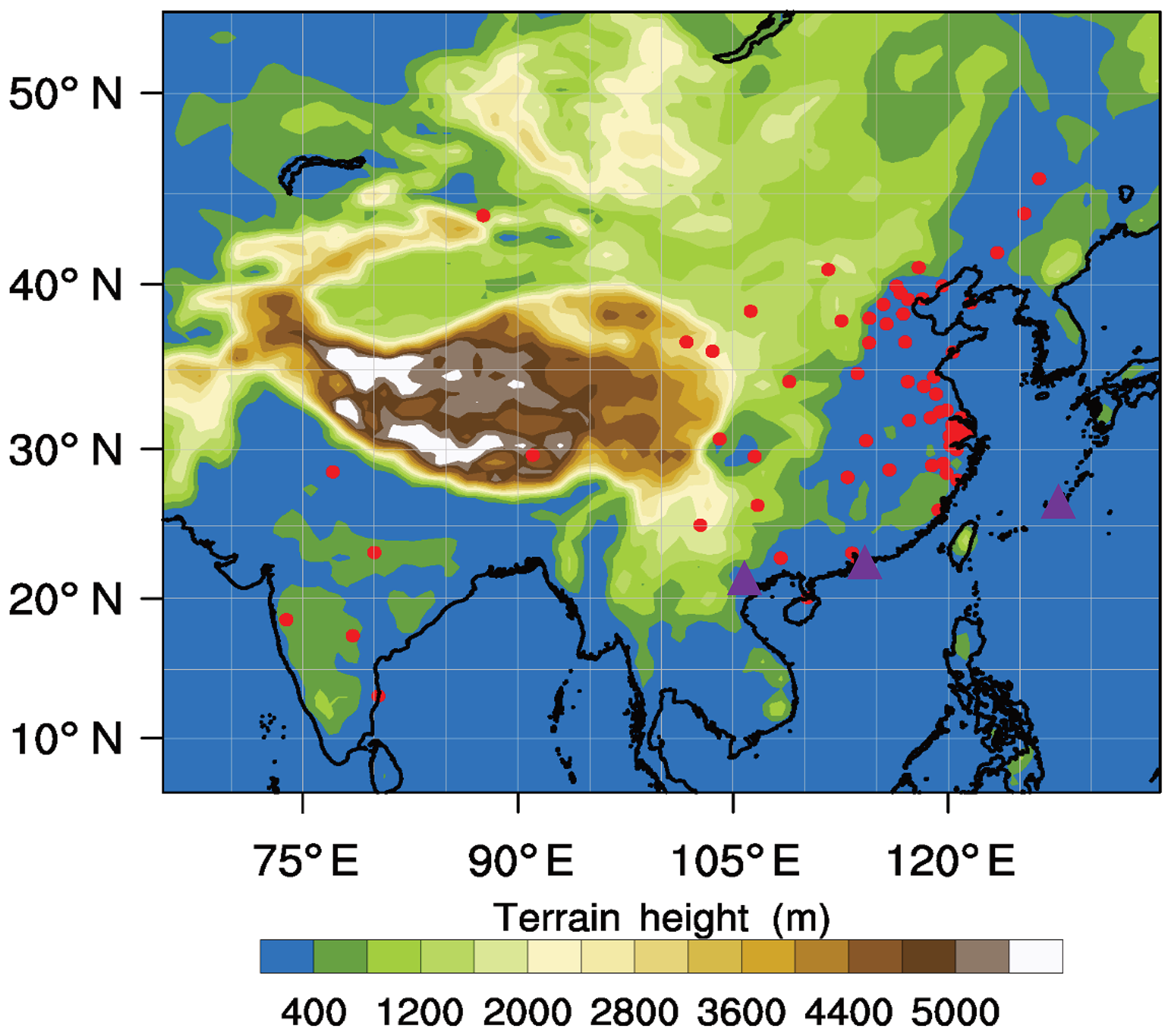
Figure 1WRF-Chem domain setting with terrain height and the locations of surface ozone observations marked by solid red circles. Solid purple triangles mark the location of ozonesonde observations.
2.1 WRF-Chem model and configurations
The fully online coupled meteorology–chemistry model WRF-Chem (Grell et al., 2005) was employed in this study using the CBMZ (carbon bond mechanism version Z; Zaveri and Peters, 1999) photochemical mechanism and the MOSAIC (Model for Simulating Aerosol Interactions and Chemistry; Zaveri et al., 2008) aerosol chemistry module. The model was configured with a horizontal grid spacing of 60 km with 27 vertical layers (from the surface to 10 hPa), covering east and south Asia (Fig. 1). The selected physical parameterization schemes follow the settings documented in Gao et al. (2016b), and they are listed in Table S1 in the Supplement. Meteorological initial and boundary conditions were obtained from the 6-hourly FNL (final analysis; NCEP, 2000) global analysis data with a resolution. The four-dimensional data assimilation (FDDA) technique was applied to limit errors in simulated meteorology. Horizontal winds, temperature, and moisture were nudged at all vertical levels. Chemical initial and boundary conditions were provided using MOZART-4 (Emmons et al., 2010) global simulations of chemical species.
Monthly anthropogenic emissions of SO2, NOx, CO, NMVOCs (nonmethane volatile organic compounds), NH3, PM2.5, PM10, BC (black carbon), and OC (organic carbon) were taken from the MIX 2010 inventory (Li et al., 2017), a mosaic Asian anthropogenic emission inventory covering both China and India. In this study, the emissions in China were updated with the MEIC (Multi-resolution Emission Inventory for China, http://www.meicmodel.org/, last access: 5 April 2020) for the year 2012. From 2012 to 2013, emissions of SO2 and NOx in China declined by 11 % and 5 %, while emissions of other species did not exhibit a significant change (Zheng et al., 2018). The MIX inventory was prepared considering five economic sectors on a grid: power, industrial, residential (heating, combustion, solvent use, and waste disposal), transportation, and agriculture. For India, SO2, BC, OC, and power plant NOx emissions were taken from the inventory developed by the Argonne National Laboratory (ANL), with the REAS (Regional Emission inventory in ASia) used to supplement missing species. Speciation mapping of VOC emissions follows the speciation framework documented in Li et al. (2014) and Gao et al. (2018). MEGAN (Model of Emissions of Gases and Aerosols from Nature; Guenther et al., 2012) version 2.04 was used to generate biogenic emissions online. Biomass burning emissions were obtained from the fourth-generation Global Fire Emissions Database (GFED4; Giglio et al., 2013). For China, industrial and power sectors are the largest two contributors to NOx emissions, while the industrial sector emits the largest quantities of NMVOCs (Li et al., 2017). For India, transportation and power sectors produce the largest quantities of NOx, while residential and transportation sectors are the largest two contributors to NMVOC emissions (Li et al., 2017). China's biogenic emissions of VOCs are estimated to be comparable to or higher than anthropogenic sources (Li and Xie, 2014; Wei et al., 2011).
2.2 Ozone tagging method and setting of source regions
O3 observed in a particular region is a mixture of O3 formed by reactions of NOx with VOCs emitted at different locations and times. The O3 tagging method has the capability to apportion contributions of different source regions to O3 concentrations observed in particular regions. The present study adopted the ozone tagging method implemented in WRF-Chem by Gao et al. (2017a), which is similar to the ozone source apportionment technology (OSAT; Yarwood et al., 1996) approach implemented in the Comprehensive Air Quality Model with Extensions (CAMx). Both O3 and its precursors from different source regions are tracked as independent variables. The ratio of formaldehyde to reactive nitrogen oxides (HCHO ∕ NOy) was used as proposed by Sillman (1995) to decide whether the grid cell is under NOx or VOC-limited conditions, and then different equations for these two conditions were selected to calculate total O3 chemical production. A detailed description of the technique is provided in Gao et al. (2017a).
The O3 tagging method attributes production of O3 and its precursors to individual geographic areas. We divided the entire modeling domain into 23 source regions, which were classified mainly using the administrative boundaries of provinces. In eastern China, each province was considered as a source region, while provinces in northeastern, northwestern, and southwestern China were lumped together (Fig. S1 in the Supplement). India was divided into two source regions (north and south), and other countries were considered separately as a whole (Fig. S1). Additionally, the chemical boundaries provided by MOZART-4 were adopted to specify inputs of O3, and the initial condition was also tracked as an independent source. The names of all source groupings are indicated in Fig. S1.
2.3 Experiment design
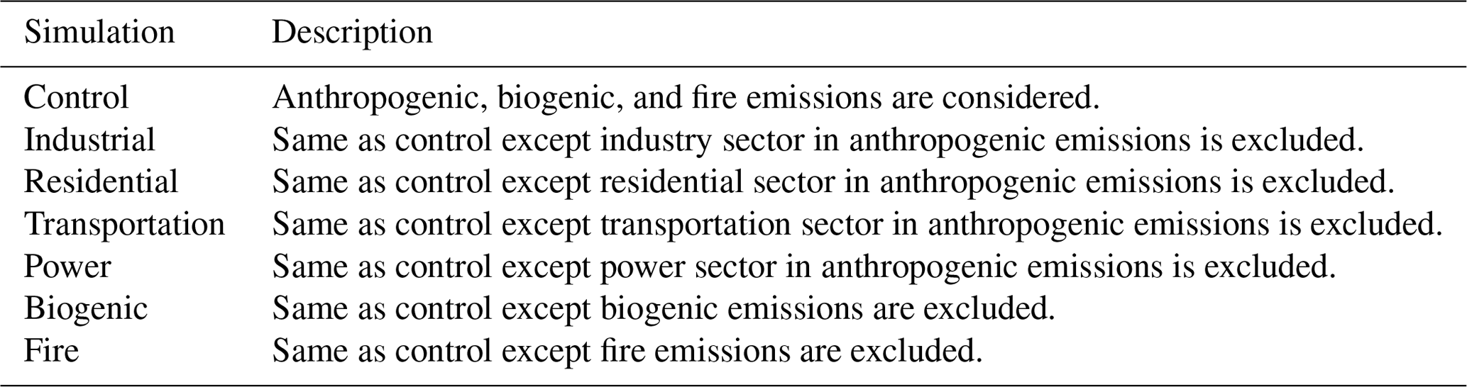
To quantify the sectoral contributions to O3, a factor separation approach (FSA) was applied to differentiate two model simulations: one with all emission sources considered and the other with some emission sources excluded. Table 1 summarizes the different sets of simulations conducted in this study. In addition to the control case, a series of sensitivity studies were performed, in which industrial, residential, transport, power, biogenic, and fire emissions were separately excluded (Table 1). For each case, the entire year of 2013 was simulated.
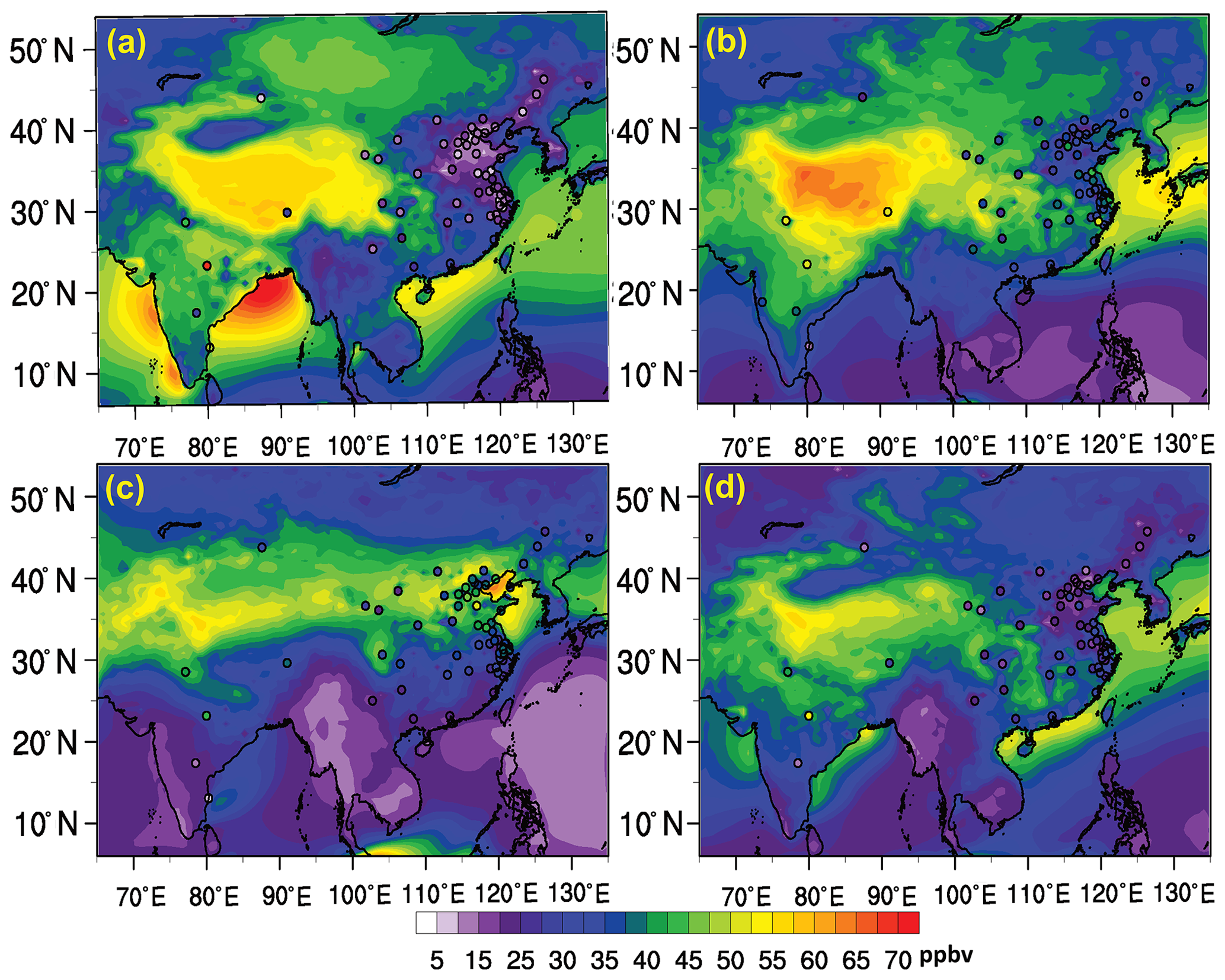
Figure 2Spatial distribution of simulated and observed seasonal mean ozone concentrations for winter (a), spring (b), summer (c), and autumn (d).
2.4 Measurements
Surface air pollutants in China are measured and recorded by the Ministry of Ecology and Environment (formerly the Ministry of Environmental Protection), and the data are accessible on the China National Environmental Monitoring Center (CNEMC) website (http://106.37.208.233:20035/, last access: 5 April 2020). This nationwide network was initiated in January 2013, and this dataset was used to evaluate model performance. This dataset has been extensively employed in previous studies to understand the spatial and temporal variations in air pollution in China (Hu et al., 2016; Lu et al., 2018a) and to reduce uncertainties in estimates of health and climate effects (Gao et al., 2017b). Measurements of air pollutants from the MAPAN (Modeling Air Pollution and Networking) network set up by the Indian Institute of Tropical Meteorology (IITM) under project SAFAR (System of Air Quality and weather Forecasting And Research; Beig et al., 2015) were used in the present study to evaluate the model performance over India. To further evaluate how the model performed in capturing the vertical distributions of O3, we used data from ozonesonde records obtained from the World Ozone and Ultraviolet Radiation Data Centre website (https://woudc.org/data/dataset_info.php?id=ozonesonde, last access: 5 April 2020). Figure 1 displays the locations of the relevant surface and ozonesonde observation sites. We also evaluated the spatial distribution of NO2 columns using the KNMI DOMINO (Dutch OMI NO2) daily level-2 products of the tropospheric NO2 column (http://www.temis.nl/index.php, last access: 5 April 2020), with the row anomaly removed (according to operational flagging), solar zenith angles less than 80∘, and cloud fraction less than 0.2. The model results were sampled according to selected satellite data on a pair-to-pair basis. The matched model results were transformed by applying the OMI averaging kernel to the modeled vertical profiles of NO2 concentrations.
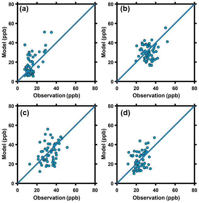
Figure 3Scatterplot of simulated and observed seasonal mean ozone concentrations for winter (a), spring (b), summer (c), and autumn (d).
We evaluated the spatial distribution of simulated seasonal mean (winter months are January, February, and December (DJF); spring months are March, April, and May (MAM); summer months are June, July, and August (JJA); autumn months are September, October, and November (SON)) O3 concentrations by comparing model results with observations (filled circles in Fig. 2) for 62 cities in China and India. The model captures the spatiotemporal patterns of O3 in east China, with lower values in autumn (Fig. 2d) and winter (Fig. 2a) and enhanced levels in spring (Fig. 2b) and summer (Fig. 2c). However, O3 concentrations are overestimated by the model in Central, Northwest and Southwest China for all seasons (Fig. 2). Hu et al. (2016) also reported that their model tends to predict higher O3 concentrations for these regions. Scatterplots of simulated and observed O3 for all four seasons suggest that the model overestimates O3 in most sites during winter and exhibits better performance during other seasons (Fig. 3). Figure S2 indicates that modeled NO2 column values in east China are not as high as observed, but the model overpredicts the NO2 column in Central China and most parts of India, which could partly explain the overestimation of O3 in Central China.
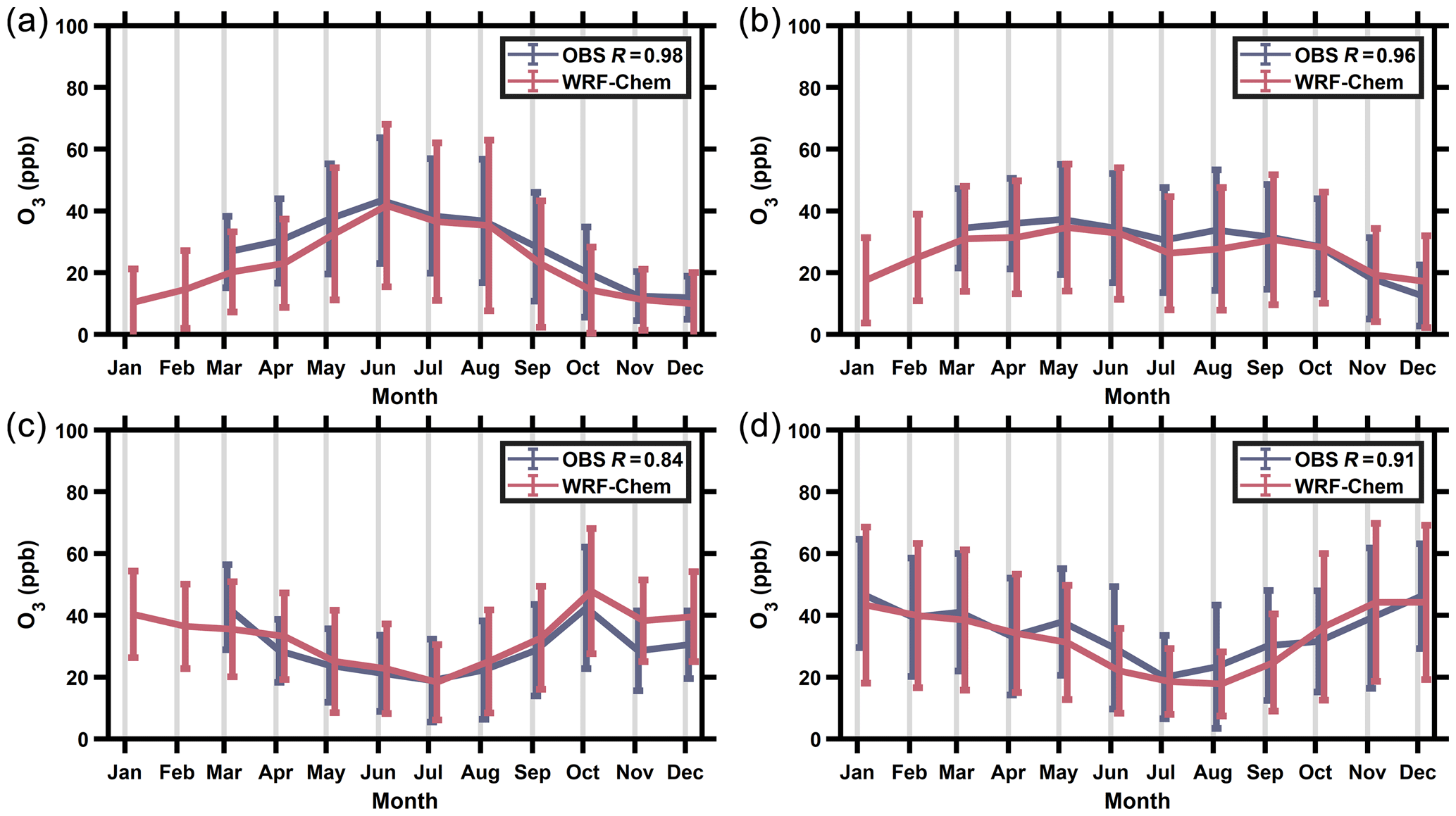
Figure 4Observed and simulated monthly mean O3 concentrations averaged for the North China Plain (NCP) (a), Yangtze River Delta (YRD) (b), Pearl River Delta (PRD) (c), and India (d).
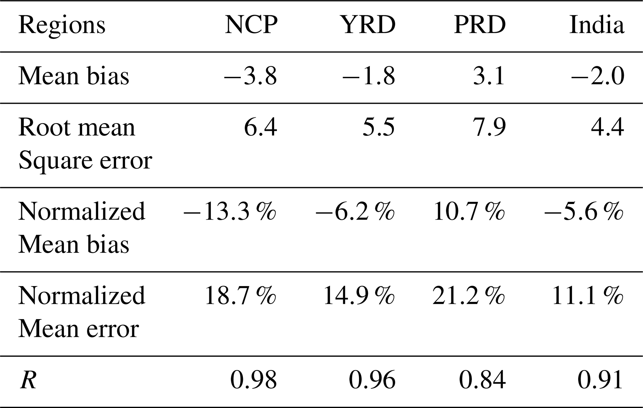
We conducted a further site-by-site evaluation of monthly mean O3 concentrations, and we grouped stations into four major densely populated regions, namely North China Plain (NCP), Yangtze River Delta (YRD), Pearl River Delta (PRD), and India. The seasonality of observed O3 concentrations is reproduced well in these four regions (Fig. 4), although concentrations are underestimated in the NCP in spring. O3 concentrations in October, November, and December in the PRD region are overestimated by the model. The correlation coefficients between model and observations range between 0.84 and 0.98. Detailed model evaluation statistics are documented in Table 2. In Beijing, the daily maximum 8 h average (MDA8) O3 concentrations are well captured by the model (Fig. S3), except that the model is biased towards low values in spring. Stronger NOx titrations (underestimation of O3 during the night; Fig. S4) are found in the model results for the NCP and YRD regions in spring, which can partly explain the underestimation of O3 in spring in the NCP and PRD (Fig. S4). The simulated magnitudes of O3 in India are generally consistent with observations, though lower in central India and in May. The high concentrations of O3 in India were not captured by the model mainly because of the large underestimation in Jabalpur (central India) with its complex terrain. The model's coarse resolution and poor capability of resolving strong spatial heterogeneity in land types within a small area have led to this mismatch, which was also found in Sharma et al. (2017). Figure 4 also suggests that the seasonal behavior of O3 in these four major regions exhibits distinctive patterns, discussed in detail in Sect. 4.
In this work, ozonesonde measurements from the Hong Kong Observatory (HKO), Japan Meteorological Agency (JMA), and the Hydro-Meteorological Service of Vietnam (HSV; locations marked in purple in Fig. 1) were used. Wintertime near-surface O3 concentrations are overestimated for HKO (Fig. S5), while vertical variations are satisfactorily captured by the model. Comparisons of near-surface O3 precursors suggest that CO concentrations are underestimated in all the regions (Fig. S6), which could be explained by an underestimate of CO emissions (Wang et al., 2011). The coarse grid resolution of the model might provide another reason for this underestimation, as the observation sites in China are located mostly in urban areas. Underestimates of CO concentrations are also reported for many sites in India (Hakim et al., 2019). The effects of underestimated CO on O3 were found to be small, but the underestimation of CO may lead to bias in methane lifetime values (Strode et al., 2015), which is beyond the discussion of regional pollution in this study. Simulated NO2 concentrations are slightly overestimated in the NCP but are underestimated in the PRD (Fig. S6). Despite these issues, the model still captures the seasonal behavior of O3 in different regions, and we do not expect the model biases to change the major findings of the present study.
4.1 Seasonality of surface O3 in different regions
Comparisons between modeled and observed near-surface O3 concentrations for different regions suggest distinctive seasonal patterns (Fig. 4). Over the NCP, near-surface O3 exhibits an inverted V-shaped pattern, with maximum O3 concentrations in summer and minimum in winter (Fig. 4). Over the YRD, O3 presents a bridge shape, with relatively higher concentrations in spring, summer, and autumn (Fig. 4). O3 concentrations over the PRD peak in autumn, with a minimum in summer (Fig. 4). Similarly, O3 over India exhibits a minimum in summer, with highest concentrations in winter (Fig. 4).
China and India are influenced largely by monsoonal climates (Wang et al., 2001), and the seasonality of O3 in different regions is affected by wind pattern reversals related to the winter and summer monsoon systems (Lu et al., 2018b). Various monsoon indices have been proposed to describe the major features of the Asian monsoon, based on pressure, temperature, and wind fields, etc. In the present study, we adopted the dynamical normalized seasonality monsoon index (DNSMI) developed by Li and Zeng (2002) to explore the influence of monsoon intensity on the seasonal behavior of O3 in the boundary layer in different regions of China and India. DNSMI is defined as follows:
in which V1 and Vi represent the wind vectors in January and wind vectors in month i, respectively. denotes the mean of wind vectors in January and July. The norm of a given variable is defined as
where S represents the spatial area of each model grid cell. More detailed information on the definition is presented in Li and Zeng (2002).
This definition of monsoon proposed by Li and Zeng (2002) focuses on wind vectors, representing the intensity of wind direction alternation from winter to summer. In winter, northwesterly winds are predominant; then higher DNSMI values indicate stronger alternation of wind directions. For example, DNSMI values are higher than 5 in coastal regions of South China and most environments in India (Fig. 5c), suggesting that these regions are influenced largely by the summer monsoon. The spatial distribution of monsoon precipitation in Fig. S7c also indicates that most areas of India and South China are influenced by the summer monsoon. The alternation of wind vectors (Fig. 5) and precipitation (Fig. S7) from winter to summer results in changes in upwind areas and abundance of O3 precursors, modulating the severity of O3 pollution. In summer, the southerly winds containing clean maritime air masses serve to reduce the intensity of pollution in regions that are affected largely by the summer monsoon (e.g., most regions over India and coastal regions over China). Besides, the summer monsoon can bring about cloudy and rainy weather conditions (Fig. S7; removement of ozone precursors), weaker solar radiation, and lower temperature (Lu et al., 2018b), which are not conducive to the photochemical production of O3 (Lu et al., 2018b; Tang et al., 2013). The onset of the summer monsoon is also associated with strong air convergence and uplift, which is not favorable for the accumulation of O3 and its precursors (Lu et al., 2018b).

Figure 5Modeled mean near-surface wind fields (winds at 10 m a.g.l.) and the monsoon index in the boundary layer (0–1.5 km) for winter (December, January, and February; a), spring (March, April, and May; b), summer (June, July, and August; c), and autumn (September, October, and November; d).
North China is less influenced by the summer monsoon as suggested by the insignificant precipitation in summer (Fig. S7c). East China and South China are more affected as suggested by DNSMI values higher than 0.5 and more abundant precipitation (Figs. 5c and S7c). High temperature and stronger solar radiation in summer favor the photochemical production of O3. As a result, O3 concentrations in the NCP peak in summer, exhibiting an inverted V-shaped pattern (Fig. 4a). The YRD region is affected moderately by the summer monsoon, with DNSMI values greater than 0.6 and mean precipitation greater than 7 mm d−1 (Figs. 5c and S7c). The upwind sources for the YRD in summer include both polluted (South China) and clean (ocean) regions. Thus, the inhibition of O3 formation in the YRD due to the summer monsoon does not lead to the annual minima in summer. Because of the favorable weather conditions (increasing temperature and solar radiation and low precipitation) in spring and autumn (Fig. S7d), the seasonality of O3 in the YRD exhibits a bridge shape, consistent with previous observations within this region (Tang et al., 2013). In addition, southerly winds might bring O3 and its precursors from the YRD region in summer (Fig. 5c), which is further quantified in Sect. 4.3. For India and the PRD region, the alternation of wind fields and precipitation begins as spring approaches (Figs. 5 and S7). As a result, O3 concentrations decline in response to input of cleaner air from the ocean and more precipitation. As summer arrives, the intensity of the monsoon reaches its maximum (Figs. 5c and S7) and concentrations of O3 in both India and South China decline to reach their annual minima (Fig. 4c and d). As wind direction changes over the east coast of China from summer to autumn, O3 peaks in autumn in South China can also be attributed to the outflow of O3 and its precursors from the NCP and YRD regions (Fig. 5d). This contribution is discussed further in Sect. 4.3.
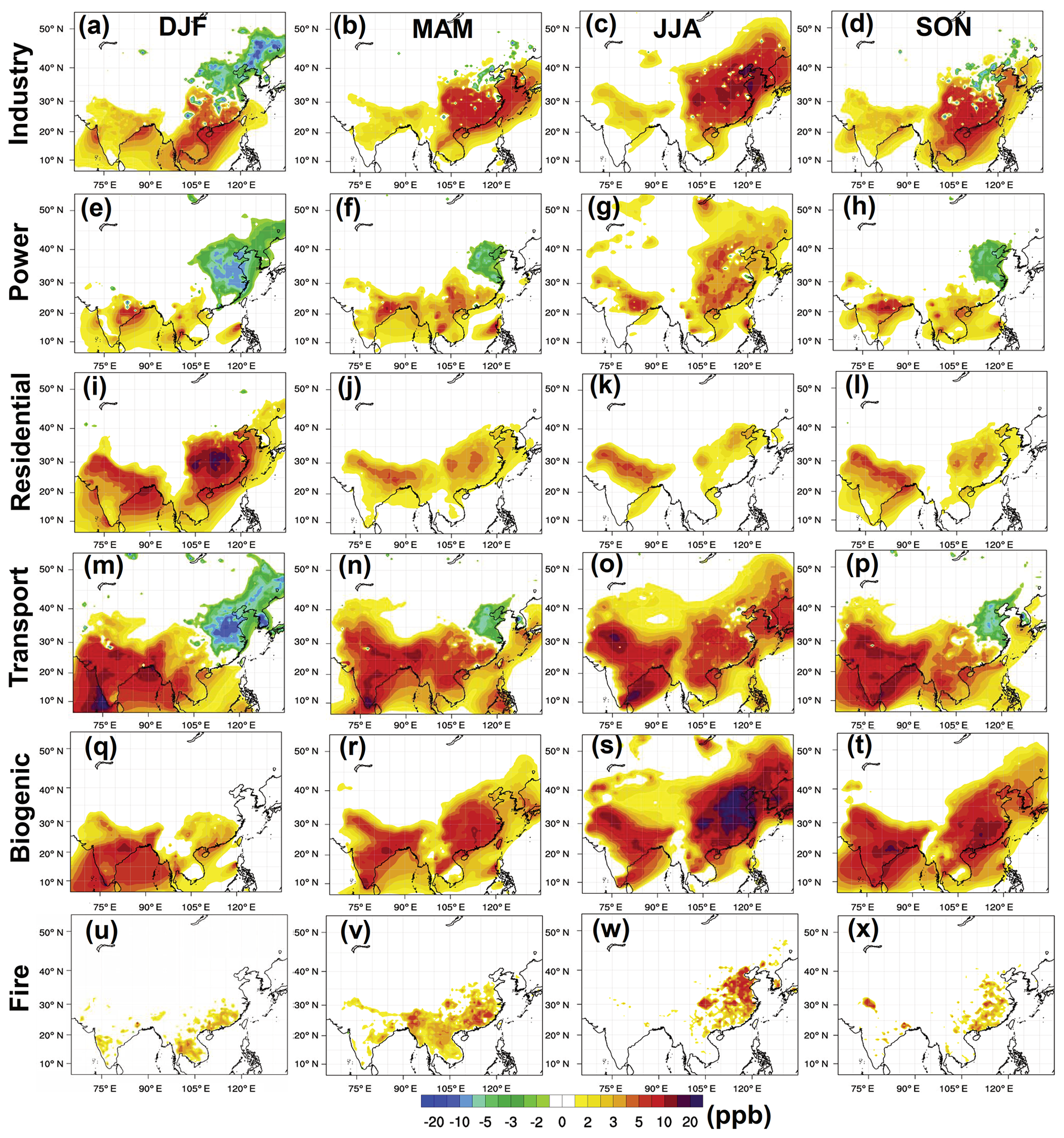
Figure 6Distributions of the contributions to near-surface ozone averaged for winter, spring, summer, and autumn from industry (a–d), power (e–h), residential (i–l), transport (m–p), biogenic (q–t), and fire and biomass burning (u–x) emissions.
4.2 O3 sensitivity to emissions from individual source sectors
O3 in the troposphere is formed through complex nonlinear processes involving emissions of NOx and VOCs from various anthropogenic, biogenic, and biomass burning sources. We illustrate in Fig. 6 the sensitivity of seasonal mean O3 concentrations in both China and India to individual source sectors, showing patterns that offer important implications for seasonal O3 control strategies in some highly polluted regions. The sensitivity is defined as the responses of O3 concentration to the elimination of each source sector (O3 with all emissions−O3 without each sector).
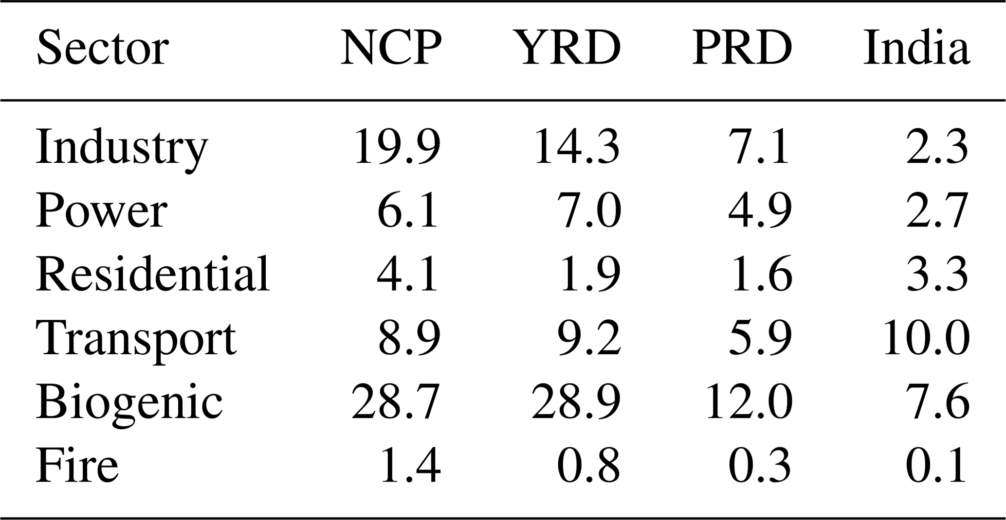
Table 3Sensitivity of seasonal O3 to emission sectors for different regions (ppb).
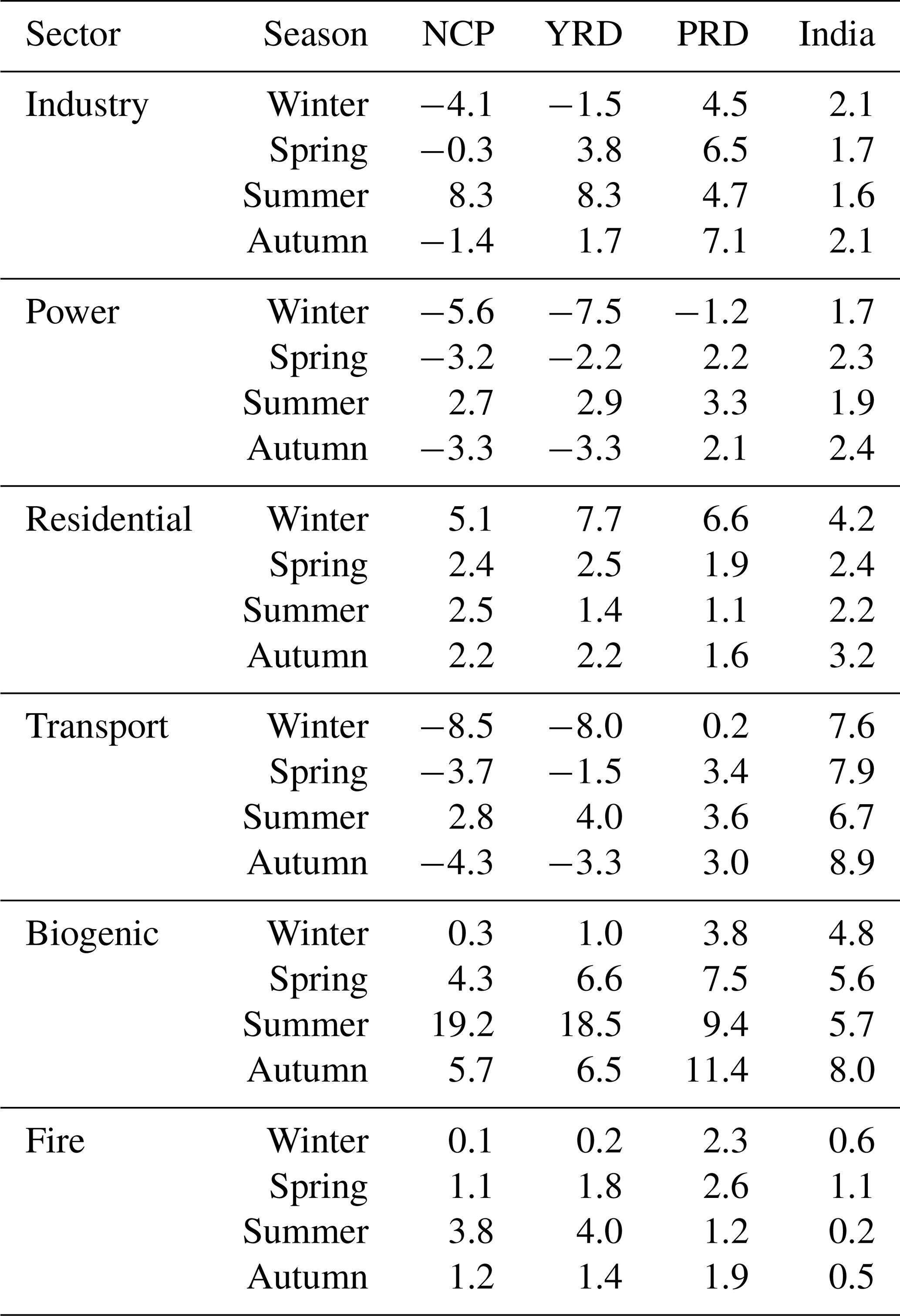
For China, summer O3 formation is more sensitive to industrial sources than to other anthropogenic sources, including power, residential, and transport (Fig. 6c and Table 3). Emissions from the industrial sector are responsible for an enhancement of O3 concentrations by more than 8 ppb in the NCP and YRD regions in summer (Fig. 6c and Table 3). Using a similar approach, Li et al. (2017) reported that the contribution to O3 from industrial sources exceeded 30 µg m−3 (∼15 ppb) in highly industrialized areas, including Hebei, Shandong, and Zhejiang during an episode in May. Li et al. (2016) concluded that the industrial sector plays the most important role in O3 formation in Shanghai, accounting for more than 35 % of observed concentrations. Adopting a source-oriented chemical transport model, Wang et al. (2019) demonstrated that the industrial source contributes 36 %, 46 %, and 29 % to nonbackground O3 in Beijing, Shanghai, and Guangdong, respectively.
In the NCP and YRD regions, O3 formation in winter, spring, and autumn reflects negative sensitivity to the transport and power sectors (Fig. 6 and Table 3). These two sectors dominate emissions of NOx in China (Li et al., 2017). Removing these sectors would lead to increases in O3 in VOC-limited regions of east China in winter, spring, and autumn (fewer biogenic emissions of VOCs in these seasons; Fu et al., 2012). The ratio of formaldehyde to reactive nitrogen (HCHO ∕ NOy) is widely used to determine the O3 production sensitivity with a critical value of 0.28 (Sillman, 1995; Zhao et al., 2009). Figure S8 indicates that east China is VOC-limited in winter, spring, and autumn. Urban regions in China are still VOC-limited (Fig. S8c; Fu et al., 2012; Jin et al., 2017) in summer, leading to negligible or negative sensitivity to the transport and power sectors as shown in Fig. 6g and o. In other regions of east China, removing transport and power sources would lead to an increase in O3 concentrations by about 4 ppb in summer. The negative sensitivity of O3 to the transport and power sectors may also be caused by the nighttime titration effects. In winter, daytime (12:00–18:00 local time) mean O3 also exhibits negative sensitivity to the transportation sector and a similar distribution to daily mean O3 sensitivity (Fig. S9a and b), suggesting nighttime titration effects might not be the major reason for the O3 negative sensitivity in winter. However, daytime mean and daily mean O3 exhibit different patterns of sensitivity to the transportation sector in highly urbanized regions in summer, which could be related to nighttime titration effects. As indicated in Fig. S10, O3 sensitivity to transportation sector in Beijing is positive during the day but negative during the night.
Including biogenic emissions results in an increase in summer mean O3 concentrations by more than 18 ppb in the NCP and YRD regions (Fig. 6s and Table 3). The high sensitivity of O3 to biogenic emissions is associated with the massive quantity of VOCs emitted from the biosphere (Table S2). The mass of biogenic VOCs is comparable to the mass emitted from all anthropogenic sectors in China and greater than anthropogenic VOCs in India (Table S2). Using a similar approach, Li et al. (2018) found that biogenic emissions contributed 8.2 ppb in urban Xi'an. Other source apportionment studies indicate that the contribution of biogenic emissions to O3 formation is about 20 % in China (Li et al., 2016; Wang et al., 2019). The enhancements due to biogenic emissions are larger over South China during winter, and the significantly impacted regions extend northwards in spring and autumn (Fig. 6q–t). Biomass burning emissions lead to relatively lower O3 enhancements over China in winter, but they are responsible for an appreciable contribution to O3 pollution (∼4 ppb) in east China in summer (Fig. 6w and Table 3). Li et al. (2016) suggested that biomass burning sources contribute about 4 % to O3 formation in the YRD region in summer. The enhancement due to biomass burning estimated by Lu et al. (2019) using a different model indicates lower values in east China.
For India, O3 formation is most sensitive to the transport vehicle sector (∼8 ppb) in all seasons (Table 3), slightly higher than it is to the biogenic source (Fig. 6m–p and Table 3). Among other sectors, the sensitivity of O3 formation to the residential sector is significant in winter as the residential sector emits the largest quantity of NMVOCs (Li et al., 2017), while the influence of biomass burning emissions is negligible.
Table 4Sensitivity of summer (July) daytime O3 to emission sectors for different regions (ppb).
To further address the issue of nighttime titration effects, we also calculated the sensitivity of daytime O3 formation in July to the different sectors, and we found that daytime O3 in the NCP and YRD are also most sensitive to industrial and biogenic emissions (Table 4). Among other anthropogenic sectors, transportation emissions play the most important role in the formation of daytime O3 in China, followed by power generation emissions (Table 4). Our results highlight the importance of industrial sources and biogenic emissions in O3 formation in east China, consistent with the conclusions of Li et al. (2017). The significance of other sectors demonstrated by Li et al. (2017) partly disagrees with the current findings. Conclusions from Li et al. (2017) rely on simulations of a 1-week episode in May, while our results provide more information considering different seasons and different highly polluted regions.

Figure 7Contributions to monthly mean ozone in NCP (a), YRD (b), PRD (c), and India (d) from different source regions (NCP: Beijing, Tianjin, Hebei, Shandong, and Henan; YRD: Anhui, Jiangsu, Shanghai, and Zhejiang; SE China: Jiangxi, Fujian, and Taiwan; Central China: Hunan and Hubei; South China: Guangxi and Hainan).
4.3 O3 contribution from individual source regions
The sensitivity of O3 pollution to individual source sectors discussed in the previous section provides a quantitative understanding of the relative importance of individual source sectors. Additionally, information on the contribution of individual source regions to O3 pollution should provide useful inputs for O3 control strategies. Because of the large computational costs of sensitivity simulations, we employed the tagging method to examine contributions to O3 pollution from individual source regions. Figure 7 presents monthly mean concentrations of O3 averaged over the NCP, YRD, PRD, and India, with contributions from individual source regions.
The NCP region is influenced largely by sources outside China, especially in wintertime, which might be attributed to less local production and a longer O3 lifetime in winter. In winter, sources outside China are responsible for more than 75 % of O3 formation in the NCP region. However, this contribution declines to about 50 % as summer approaches. Using the tagged tracer method with a global chemical transport model, Nagashima et al. (2010) suggested that sources outside China contributed about 60 % and 40 % of surface O3 in north China in spring and summer, respectively. Our estimate for the contributions of sources outside China in these two seasons suggests slightly higher values: 73 % and 51 % (Table 5). In summer, NCP local sources contribute about 31 %, with an additional 8 % from Northwest China.
Table 5Long-range transport, local, and regional source contributions for seasonal mean O3 for different regions.
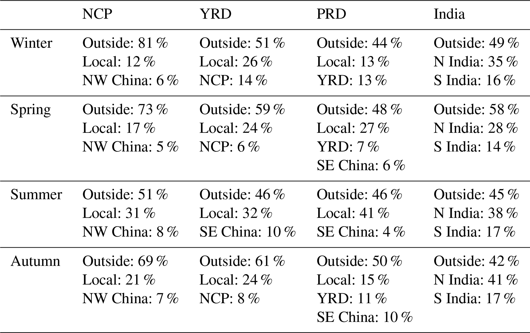
Outside sources represent sources outside China for the discussed three regions in China, and sources outside India for India, also including transport from the upper boundary of the model; NCP: Beijing, Tianjin, Hebei, Shandong, and Henan; YRD: Anhui, Jiangsu, Shanghai, and Zhejiang; SE China: Jiangxi, Fujian, and Taiwan; Central China: Hunan and Hubei; South China: Guangxi and Hainan.
For the YRD region, local emissions contribute 32 % of O3 formation in summer, but the contribution declines by 8 percentage points in spring and autumn (Table 5). The contribution of sources outside China decreases greatly in summer (46 %), leading to a small summer O3 trough. The source apportionment results in Nagashima et al. (2010) also indicated that the contribution of sources outside China to O3 in the Yangtze River basin decreases significantly from spring to summer (44 % to 30 %). The relatively lower contribution from sources outside China is associated with the prevailing winds and cleaner air from the ocean in summer (Fig. 5c). In addition to local sources, we further identified that the major source region for O3 in the YRD region is the NCP in winter, spring, and autumn (14 %, 6 %, and 8 %, respectively). In summer, the major source region of O3 in the YRD region is Southeast China (10 %). Gao et al. (2016a) concluded that YRD local emissions contribute 13.6 %–20.6 % of daytime O3 under different wind conditions, and the contribution of superregional sources (outside) ranges from 32 % to 34 % in May. In Hangzhou (a megacity within the YRD), source apportionment results reveal that long-range transport contributes 36.5 % of daily maximum O3 with the overall contribution dominated by local sources (Li et al., 2016).
O3 concentrations in the YRD region are influenced largely by the summer monsoon, and the prevailing winds from the ocean result in a minimum contribution from polluted regions. The estimated contribution of sources outside China declines to 46 % in summer, which agrees well with the 47 % value inferred from Nagashima et al. (2010). Li et al. (2012) applied the OSAT tool in the CAMx to apportion O3 sources in South China, and they reported that superregional sources contributed 55 % and 71 % of monthly mean O3 in summer and autumn, respectively. They also pointed out that regional and local sources play more important roles in O3 pollution episodes (Li et al., 2002). The contribution of local sources peaks in summer (41 %), exceeding the local contribution in the NCP and YRD regions. As discussed in Sect. 4.1, the outflow of O3 and its precursors from the NCP and YRD regions might play an important role in peak autumn O3 in the YRD (Fig. 5d), as wind direction switches from summer to autumn. We identified the major upwind regions for the PRD in autumn as the YRD (11 %) and Southeast China (10 %). From summer to autumn, the contribution of YRD sources to the PRD increases from 2 % to 11 %. For India, O3 concentrations are dominated by sources outside India and sources in North India (Fig. 7d). In winter, sources outside India contribute 49 %, while sources in North India contribute 38 %.
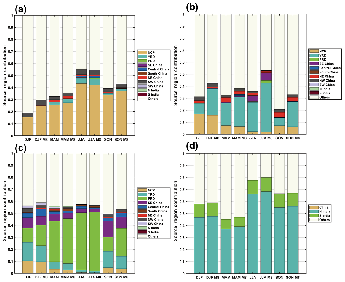
Figure 8Contributions to seasonally daily mean ozone (DJF, MAM, JJA, and SON) and MDA8 ozone (DJF M8, MAM M8, JJA M8, and SON M8) in Beijing (a), Shanghai (b), Guangzhou (c), and New Delhi (d) from different source regions.
We also calculated the contributions of sources in different regions to MDA8 O3 concentrations, and we compared the results with contributions to daily mean O3. As shown in Fig. 8, the contributions of sources in different regions do not exhibit a large difference for Beijing, except that the local sources play a more important role in the formation of daytime O3 in winter (Fig. 8a). Similarly, higher contributions of local sources to the formation of daytime O3 are found for Guangzhou in autumn and for Shanghai in all seasons (Fig. 8). The contributions of sources in different regions do not show a notable difference for New Delhi, India.
The estimated contributions of sources outside China to O3 pollution in receptor regions exhibit slightly higher values than the values inferred from studies using global models (Nagashima et al., 2010; Wang et al., 2011). This might be related partly to the inconsistency between simulations from the applied regional model and boundary conditions from other global models. Global chemical transport models usually show better skills in simulating transboundary pollution.
In this study, we used a fully coupled regional meteorology–chemistry model with a horizontal grid spacing of 60 km × 60 km to study the seasonality and characteristics of sources of O3 pollution in highly polluted regions in both China and India. Both observations and model results indicate that O3 in the NCP, YRD, PRD, and India display distinctive seasonal features. Surface concentrations of O3 peak in summer in the NCP, in spring in the YRD, in autumn in the PRD, and in winter in India. These distinct seasonal features for different regions are linked to the intensity of the summer monsoon, to sources, and to atmospheric transport.
With confidence in the model's ability to reproduce the major features of O3 pollution, we examined the sensitivity of O3 pollution to individual anthropogenic emission sectors and to emissions from biogenic sources and from burning of biomass. We found that the production of O3 in summer is more sensitive to industrial and biogenic sources than to other source sectors in China, while the transportation and biogenic emissions are more important for all seasons in India. For India, in addition to transportation, the residential sector also plays an important role in winter when O3 concentrations peak. These differences in conditions between China and India suggest differences in control strategies applied to economic sectors should be implemented to minimize the sectors' resulting pollution.
Tagged simulations suggest that sources in east China play an important role in the formation of the summer O3 peak in the NCP, and sources from Northwest China should not be neglected in the control of summer O3 in the NCP. For the YRD region, prevailing winds and cleaner air from the ocean in summer lead to reduced transport from polluted regions and the major source region in addition to local sources is Southeast China. For the PRD region, the upwind region is replaced by contributions from polluted east China as autumn approaches, leading to an autumn peak. The major upwind regions in autumn for the PRD are the YRD (11 %) and Southeast China (10 %). For India, sources in North India show larger contributions than sources in South India.
The focus of our analysis is on the seasonality of O3 pollution and its sources in both China and India, with an emphasis on implications for O3 control strategies. Most previous studies focused on the analysis of episodes or monthly means for a region, while the current study presents a more comprehensive picture. For the NCP region, O3 concentrations peak in summer, during which industrial sources should be given higher priority. Besides local sources in the NCP, sources from Northwest China also play important roles. For the YRD region, O3 concentrations in spring, summer, and autumn are equally important, showing appreciable sensitivity to the industrial sources. In addition to local sources, sources from the NCP should be considered for the control of O3 in spring and autumn, while sources from Southeast China should be considered in summer. For the PRD region, O3 concentrations peak in spring and autumn, during which reducing industrial and transportation sources could be more effective. In both spring and autumn, sources from the YRD and Southeast China show appreciable contributions to O3 pollution in the PRD. For India, O3 pollution is more serious in winter, during which controlling residential and transport sources in North India could be more effective.
However, uncertainties remain in the conclusions resulting from the assumptions and methodology adopted in this study. The zero-out method is computationally inefficient. It is a sensitivity method and does not provide the source contribution for nonlinear systems, as the sum of impacts of all sources does not equal the total concentration (Yarwood et al., 2007). Although there is no perfect source apportionment technique for nonlinear systems, a reasonable method that tracks mass contributions and accounts for chemical nonlinearity can provide additional information in terms of the design of control strategies (Yarwood et al., 2007). In the tagging method, the photochemical indicator HCHO ∕ NOy with a threshold of 0.28 (Sillman, 1995) was used to determine NOx- or VOC-limited conditions, which can also result in uncertainties in the results. Several other indicators have been proposed to indicate photochemical sensitivity, including O3 ∕ NOx and O3 ∕ NOy. However, the robustness of these indicators can vary with ambient conditions and locations (Andreani-Aksoyoglu et al., 2001). Zhang et al. (2009) recommended using multiple indicators rather than a single one to reduce uncertainties. Wang et al. (2019) suggested that the use of a single threshold for these indicators is insufficient, as O3 can be sensitive to both NOx and VOCs. A three-regime O3 attribution technique was developed by Wang et al. (2019) to address this problem. Additionally, although comparisons are shown for daytime mean and daily mean, most conclusions in this study are based on seasonal mean (both daytime and nighttime) O3, while many previous studies have investigated sources of 8 h or daily maximum O3. As illustrated in Li et al. (2016), the dominant contribution to nighttime O3 is associated with long-range transport. All of these factors contribute to uncertainties in the results of source apportionment but should not downplay the significance of current findings in terms of policy implications.
The measurements and model simulation data can be accessed through contacting the corresponding authors.
The supplement related to this article is available online at: https://doi.org/10.5194/acp-20-4399-2020-supplement.
MG and MBM designed the study; MG performed model simulations and analyzed the data with help from JG, BZ, RK, XL, SS, YZ, BJ, PW, and PS; GB, JH, QY, and HZ provided measurements. MG and MBM wrote the paper with inputs from all other authors.
The authors declare that they have no conflict of interest.
This work is supported by the special fund of the Key Laboratory for Aerosol-Cloud-Precipitation of China Meteorological Administration, Nanjing University of Information Science and Technology (KDW1901); Harvard Global Institute; special fund of the State Key Joint Laboratory of Environmental Simulation and Pollution Control (19K03ESPCT); Natural Science Foundation of Guangdong Province (no. 2019A1515011633); National Natural Science Foundation of China Major Research Plan (integrated project; grant no. NSFC91843301); and National Key Research and Development Programme – Science, Technology, and Innovation Cooperation with Hong Kong, Macau, and Taiwan (2017YFE0191000).
This research has been supported by the special fund of the Key Laboratory for Aerosol-Cloud-Precipitation of China Meteorological Administration, Nanjing University of Information Science and Technology (KDW1901); Harvard Global Institute; special fund of the State Key Joint Laboratory of Environmental Simulation and Pollution Control (19K03ESPCT); Natural Science Foundation of Guangdong Province (no. 2019A1515011633); National Natural Science Foundation of China Major Research Plan (integrated project; grant no. NSFC91843301); and National Key Research and Development Programme – Science, Technology, and Innovation Cooperation with Hong Kong, Macau, and Taiwan (2017YFE0191000).
This paper was edited by Hailong Wang and reviewed by two anonymous referees.
Andreani-Aksoyoglu, S., Lu, C. H., Keller, J., Prevot, A. S. H., and Chang, J. S.: Variability of indicator values for ozone production sensitivity: a model study in Switzerland and San Joaquin Valley (California), Atmos. Environ., 35, 5593–5604, https://doi.org/10.1016/S1352-2310(01)00278-3, 2001.
Beig, G., Gunthe, S. and Jadhav, D. B.: Simultaneous measurements of ozone and its precursors on a diurnal scale at a semi urban site in India, J. Atmos. Chem., 57, 239–253, https://doi.org/10.1007/s10874-007-9068-8, 2007.
Beig, G.: GAW Report No. 217, System of Air Quality Forecasting and Research (SAFAR-INDIA), World Meteorological Organization, 51 pp., 2015.
Chameides, W. L., Kasibhatla, P. S., Yienger, J., and Levy II, H.: Growth of Continental-scale Metro-Agro-Plexes, Regional Ozone Pollution, and World Food Production, Science, 264, 74–77, 1994.
Cheng, N., Li, Y., Zhang, D., Chen, T., Sun, F., Chen, C., and Meng, F.: Characteristics of Ground Ozone Concentration over Beijing from 2004 to 2015: Trends, Transport, and Effects of Reductions, Atmos. Chem. Phys. Discuss., https://doi.org/10.5194/acp-2016-508, 2016.
De Smedt, I., Stavrakou, T., Mller, J. F., Van Der A, R. J., and Van Roozendael, M.: Trend detection in satellite observations of formaldehyde tropospheric columns, Geophys. Res. Lett., 37, L18808, https://doi.org/10.1029/2010GL044245, 2010.
Duncan, B. N., Lamsal, L. N., Thompson, A. M., Yoshida, Y., Lu, Z., Streets, D. G., Hurwitz, M. M., and Pickering, K. E.: A space-based, high-resolution view of notable changes in urban NOx pollution around the world (2005–2014), J. Geophys. Res.-Atmos., 121, 976–996, 2016.
Emmons, L. K., Walters, S., Hess, P. G., Lamarque, J.-F., Pfister, G. G., Fillmore, D., Granier, C., Guenther, A., Kinnison, D., Laepple, T., Orlando, J., Tie, X., Tyndall, G., Wiedinmyer, C., Baughcum, S. L., and Kloster, S.: Description and evaluation of the Model for Ozone and Related chemical Tracers, version 4 (MOZART-4), Geosci. Model Dev., 3, 43–67, https://doi.org/10.5194/gmd-3-43-2010, 2010.
Fu, J. S., Dong, X., Gao, Y., Wong, D. C., and Lam, Y. F.: Sensitivity and linearity analysis of ozone in East Asia: The effects of domestic emission and intercontinental transport, J. Air Waste Manage., 62, 1102–1114, https://doi.org/10.1080/10962247.2012.699014, 2012.
Gao, J., Zhu, B., Xiao, H., Kang, H., Hou, X., and Shao, P.: A case study of surface ozone source apportionment during a high concentration episode, under frequent shifting wind conditions over the Yangtze River Delta, China, Sci. Total Environ., 544, 853–863, https://doi.org/10.1016/j.scitotenv.2015.12.039, 2016a.
Gao, M., Carmichael, G. R., Wang, Y., Saide, P. E., Yu, M., Xin, J., Liu, Z., and Wang, Z.: Modeling study of the 2010 regional haze event in the North China Plain, Atmos. Chem. Phys., 16, 1673–1691, https://doi.org/10.5194/acp-16-1673-2016, 2016b.
Gao, M., Saide, P. E., Xin, J., Wang, Y., Liu, Z., Wang, Y., Wang, Z., Pagowski, M., Guttikunda, S. K. and Carmichael, G. R.: Estimates of Health Impacts and Radiative Forcing in Winter Haze in Eastern China through Constraints of Surface PM2.5 Predictions, Environ. Sci. Technol., 51, 2178–2185, https://doi.org/10.1021/acs.est.6b03745, 2017b.
Gao, M., Han, Z., Liu, Z., Li, M., Xin, J., Tao, Z., Li, J., Kang, J.-E., Huang, K., Dong, X., Zhuang, B., Li, S., Ge, B., Wu, Q., Cheng, Y., Wang, Y., Lee, H.-J., Kim, C.-H., Fu, J. S., Wang, T., Chin, M., Woo, J.-H., Zhang, Q., Wang, Z., and Carmichael, G. R.: Air quality and climate change, Topic 3 of the Model Inter-Comparison Study for Asia Phase III (MICS-Asia III) – Part 1: Overview and model evaluation, Atmos. Chem. Phys., 18, 4859–4884, https://doi.org/10.5194/acp-18-4859-2018, 2018.
Ghude, S. D., Jena, C., Chate, D. M., Beig, G., Pfister, G. G., Kumar, R., and Ramanathan, V.: Reductions in India's crop yield due to ozone, Geophys. Res. Lett., 41, 5685–5691, https://doi.org/10.1002/2014GL060930.Received, 2014.
Ghude, S. D., Jain, S. L., Arya, B. C., Beig, G., Ahammed, Y. N., Kumar, A. and Tyagi, B.: Ozone in ambient air at a tropical megacity, Delhi: Characteristics, trends and cumulative ozone exposure indices, J. Atmos. Chem., 60, 237–252, https://doi.org/10.1007/s10874-009-9119-4, 2008.
Giglio, L., Randerson, J. T., and Van Der Werf, G. R.: Analysis of daily, monthly, and annual burned area using the fourth-generation global fire emissions database (GFED4), J. Geophys. Res.-Biogeo., 118, 317–328, https://doi.org/10.1002/jgrg.20042, 2013.
Grell, G. A., Peckham, S. E., Schmitz, R., McKeen, S. A., Frost, G., Skamarock, W. C., and Eder, B.: Fully coupled “online” chemistry within the WRF model, Atmos. Environ., 39, 6957–6975, https://doi.org/10.1016/j.atmosenv.2005.04.027, 2005.
Guenther, A. B., Jiang, X., Heald, C. L., Sakulyanontvittaya, T., Duhl, T., Emmons, L. K., and Wang, X.: The Model of Emissions of Gases and Aerosols from Nature version 2.1 (MEGAN2.1): an extended and updated framework for modeling biogenic emissions, Geosci. Model Dev., 5, 1471–1492, https://doi.org/10.5194/gmd-5-1471-2012, 2012.
Hakim, Z. Q., Archer-Nicholls, S., Beig, G., Folberth, G. A., Sudo, K., Abraham, N. L., Ghude, S., Henze, D. K., and Archibald, A. T.: Evaluation of tropospheric ozone and ozone precursors in simulations from the HTAPII and CCMI model intercomparisons – a focus on the Indian subcontinent, Atmos. Chem. Phys., 19, 6437–6458, https://doi.org/10.5194/acp-19-6437-2019, 2019.
Hilboll, A., Richter, A., and Burrows, J. P.: Long-term changes of tropospheric NO2 over megacities derived from multiple satellite instruments, Atmos. Chem. Phys., 13, 4145–4169, https://doi.org/10.5194/acp-13-4145-2013, 2013.
Hu, J., Chen, J., Ying, Q., and Zhang, H.: One-year simulation of ozone and particulate matter in China using WRF/CMAQ modeling system, Atmos. Chem. Phys., 16, 10333–10350, https://doi.org/10.5194/acp-16-10333-2016, 2016.
Jin, X., Fiore, A. M., Murray, L. T., Valin, L. C., Lamsal, L. N., Duncan, B., Folkert Boersma, K., De Smedt, I., Abad, G. G., Chance, K., and Tonnesen, G. S.: Evaluating a Space-Based Indicator of Surface Ozone-NOx-VOC Sensitivity Over Midlatitude Source Regions and Application to Decadal Trends, J. Geophys. Res.-Atmos., 122, 10439–10461, https://doi.org/10.1002/2017JD026720, 2017.
Kurokawa, J., Ohara, T., Morikawa, T., Hanayama, S., Janssens-Maenhout, G., Fukui, T., Kawashima, K., and Akimoto, H.: Emissions of air pollutants and greenhouse gases over Asian regions during 2000–2008: Regional Emission inventory in ASia (REAS) version 2, Atmos. Chem. Phys., 13, 11019–11058, https://doi.org/10.5194/acp-13-11019-2013, 2013.
Lal, S., Naja, M., and Subbaraya, B. H.: Seasonal variations in surface ozone and its precursors over an urban site in India, Atmos. Environ., 34, 2713–2724, https://doi.org/10.1016/S1352-2310(99)00510-5, 2000.
Li, J., Wang, Z., Akimoto, H., Yamaji, K., Takigawa, M., Pochanart, P., Liu, Y., Tanimoto, H., and Kanaya, Y.: Near-ground ozone source attributions and outflow in central eastern China during MTX2006, Atmos. Chem. Phys., 8, 7335–7351, https://doi.org/10.5194/acp-8-7335-2008, 2008.
Li, G., Bei, N., Cao, J., Wu, J., Long, X., Feng, T., Dai, W., Liu, S., Zhang, Q., and Tie, X.: Widespread and persistent ozone pollution in eastern China during the non-winter season of 2015: observations and source attributions, Atmos. Chem. Phys., 17, 2759–2774, https://doi.org/10.5194/acp-17-2759-2017, 2017.
Li, J. and Zeng, Q.: A new monsoon index and the geographical distribution of the global monsoons, Adv. Atmos. Sci., 20, 299–302, 2003.
Li, J., Wang, Z., Akimoto, H., Yamaji, K., Takigawa, M., Pochanart, P., Liu, Y., Tanimoto, H., and Kanaya, Y.: Near-ground ozone source attributions and outflow in central eastern China during MTX2006, Atmos. Chem. Phys., 8, 7335–7351, https://doi.org/10.5194/acp-8-7335-2008, 2008.
Li, K., Jacob, D. J., Liao, H., Shen, L., Zhang, Q., and Bates, K. H.: Anthropogenic drivers of 2013–2017 trends in summer surface ozone in China, P. Natl. Acad. Sci. USA, 116, 422–427, https://doi.org/10.1073/pnas.1812168116, 2019.
Li, L. Y. and Xie, S. D.: Historical variations of biogenic volatile organic compound emission inventories in China, 1981–2003, Atmos. Environ., 95, 185–196, https://doi.org/10.1016/j.atmosenv.2014.06.033, 2014.
Li, L., An, J. Y., Shi, Y. Y., Zhou, M., Yan, R. S., Huang, C., Wang, H. L., Lou, S. R., Wang, Q., Lu, Q., and Wu, J.: Source apportionment of surface ozone in the Yangtze River Delta, China in the summer of 2013, Atmos. Environ., 144, 194–207, https://doi.org/10.1016/j.atmosenv.2016.08.076, 2016.
Li, M., Zhang, Q., Streets, D. G., He, K. B., Cheng, Y. F., Emmons, L. K., Huo, H., Kang, S. C., Lu, Z., Shao, M., Su, H., Yu, X., and Zhang, Y.: Mapping Asian anthropogenic emissions of non-methane volatile organic compounds to multiple chemical mechanisms, Atmos. Chem. Phys., 14, 5617–5638, https://doi.org/10.5194/acp-14-5617-2014, 2014.
Li, M., Zhang, Q., Kurokawa, J.-I., Woo, J.-H., He, K., Lu, Z., Ohara, T., Song, Y., Streets, D. G., Carmichael, G. R., Cheng, Y., Hong, C., Huo, H., Jiang, X., Kang, S., Liu, F., Su, H., and Zheng, B.: MIX: a mosaic Asian anthropogenic emission inventory under the international collaboration framework of the MICS-Asia and HTAP, Atmos. Chem. Phys., 17, 935–963, https://doi.org/10.5194/acp-17-935-2017, 2017.
Li, N., He, Q., Greenberg, J., Guenther, A., Li, J., Cao, J., Wang, J., Liao, H., Wang, Q., and Zhang, Q.: Impacts of biogenic and anthropogenic emissions on summertime ozone formation in the Guanzhong Basin, China, Atmos. Chem. Phys., 18, 7489–7507, https://doi.org/10.5194/acp-18-7489-2018, 2018.
Li, Y., Lau, A. K. H., Fung, J. C. H., Zheng, J. Y., Zhong, L. J., and Louie, P. K. K.: Ozone source apportionment (OSAT) to differentiate local regional and super-regional source contributions in the Pearl River Delta region, China, J. Geophys. Res.-Atmos., 117, 1–18, https://doi.org/10.1029/2011JD017340, 2012.
Lu, X., Hong, J., Zhang, L., Cooper, O. R., Schultz, M. G., Xu, X., Wang, T., Gao, M., Zhao, Y. and Zhang, Y.: Severe Surface Ozone Pollution in China: A Global Perspective, Environ. Sci. Technol., 5, 487–494, https://doi.org/10.1021/acs.estlett.8b00366, 2018a.
Lu, X., Zhang, L., Liu, X., Gao, M., Zhao, Y., and Shao, J.: Lower tropospheric ozone over India and its linkage to the South Asian monsoon, Atmos. Chem. Phys., 18, 3101–3118, https://doi.org/10.5194/acp-18-3101-2018, 2018b.
Lu, X., Zhang, L., Chen, Y., Zhou, M., Zheng, B., Li, K., Liu, Y., Lin, J., Fu, T.-M., and Zhang, Q.: Exploring 2016–2017 surface ozone pollution over China: source contributions and meteorological influences, Atmos. Chem. Phys., 19, 8339–8361, https://doi.org/10.5194/acp-19-8339-2019, 2019.
Ma, Z., Xu, J., Quan, W., Zhang, Z., Lin, W., and Xu, X.: Significant increase of surface ozone at a rural site, north of eastern China, Atmos. Chem. Phys., 16, 3969–3977, https://doi.org/10.5194/acp-16-3969-2016, 2016.
Mills, G., Pleijel, H., Malley, C. S., Sinha, B., Cooper, O. R., Schultz, M. G., Neufeld, H. S., Simpson, D., Sharps, K., Feng, Z., Gerosa, G., Harmens, H., Kobayashi, K., Saxena, P., Paoletti, E., Sinha, V., and Xu, X.: Tropospheric Ozone Assessment Report: Present-day tropospheric ozone distribution and trends relevant to vegetation, Elem. Sci. Anth., 6–47, https://doi.org/10.1525/elementa.302, 2018.
Nagashima, T., Ohara, T., Sudo, K., and Akimoto, H.: The relative importance of various source regions on East Asian surface ozone, Atmos. Chem. Phys., 10, 11305–11322, https://doi.org/10.5194/acp-10-11305-2010, 2010.
NCEP: National Weather Service, NOAA & U.S. Department of Commerce, NCEP Final (FNL) Operational Model Global Tropospheric Analyses, continuing from July 1999, Research Data Archive at the National Center for Atmospheric Research, Computational and Information Systems Laboratory, https://doi.org/10.5065/D6M043C6, 2000.
Ohara, T., Akimoto, H., Kurokawa, J., Horii, N., Yamaji, K., Yan, X., and Hayasaka, T.: An Asian emission inventory of anthropogenic emission sources for the period 1980–2020, Atmos. Chem. Phys., 7, 4419–4444, https://doi.org/10.5194/acp-7-4419-2007, 2007.
IPCC: Climate Change 2007: Synthesis Report, Contribution of Working Groups I, II and III to the Fourth Assessment Report of the Intergovernmental Panel on Climate Change, edited by: Core Writing Team, R. K. Pachauri, and A. Reisinger, 104 pp., IPCC, Geneva, Switzerland, 2007.
Saraf, N. and Beig, G.: Long-term trends in tropospheric ozone over the Indian tropical region, Geophys. Res. Lett., 31, L05101, https://doi.org/10.1029/2003gl018516, 2004.
Sharma, A., Ojha, N., Pozzer, A., Mar, K. A., Beig, G., Lelieveld, J., and Gunthe, S. S.: WRF-Chem simulated surface ozone over south Asia during the pre-monsoon: effects of emission inventories and chemical mechanisms, Atmos. Chem. Phys., 17, 14393–14413, https://doi.org/10.5194/acp-17-14393-2017, 2017.
Sillman, S.: The use of NOy, H2O2, and HNO3 as indicators for ozone-NOx-hydrocarbon sensitivity in urban locations, J. Geophys. Res., 100, 175–188, 1995.
Stavrakou, T., Müller, J.-F., De Smedt, I., Van Roozendael, M., van der Werf, G. R., Giglio, L., and Guenther, A.: Evaluating the performance of pyrogenic and biogenic emission inventories against one decade of space-based formaldehyde columns, Atmos. Chem. Phys., 9, 1037–1060, https://doi.org/10.5194/acp-9-1037-2009, 2009.
Strode, S. A., Duncan, B. N., Yegorova, E. A., Kouatchou, J., Ziemke, J. R., and Douglass, A. R.: Implications of carbon monoxide bias for methane lifetime and atmospheric composition in chemistry climate models, Atmos. Chem. Phys., 15, 11789–11805, https://doi.org/10.5194/acp-15-11789-2015, 2015.
Sun, L., Xue, L., Wang, Y., Li, L., Lin, J., Ni, R., Yan, Y., Chen, L., Li, J., Zhang, Q., and Wang, W.: Impacts of meteorology and emissions on summertime surface ozone increases over central eastern China between 2003 and 2015, Atmos. Chem. Phys., 19, 1455–1469, https://doi.org/10.5194/acp-19-1455-2019, 2019.
Tang, H., Liu, G., Zhu, J., Han, Y., and Kobayashi, K.: Seasonal variations in surface ozone as influenced by Asian summer monsoon and biomass burning in agricultural fields of the northern Yangtze River Delta, Atmos. Res., 122, 67–76, https://doi.org/10.1016/j.atmosres.2012.10.030, 2013.
Wang, B., Wu, R., and Lau, K. M.: Interannual variability of the asian summer monsoon: Contrasts between the Indian and the Western North Pacific-East Asian monsoons, J. Climate, 14, 4073–4090, https://doi.org/10.1175/1520-0442(2001)014, 2001.
Wang, P., Chen, Y., Hu, J., Zhang, H., and Ying, Q.: Source apportionment of summertime ozone in China using a source-oriented chemical transport model, Atmos. Environ., 211, 79–90, https://doi.org/10.1016/j.atmosenv.2019.05.006, 2019.
Wang, T., Ding, A., Gao, J., and Wu, W. S.: Strong ozone production in urban plumes from Beijing, China, Geophys. Res. Lett., 33, https://doi.org/10.1029/2006GL027689, 2006.
Wang, T., Xue, L., Brimblecombe, P., Lam, Y. F., Li, L., and Zhang, L.: Ozone pollution in China: A review of concentrations, meteorological influences, chemical precursors, and effects, Sci. Total Environ., 575, 1582–1596, https://doi.org/10.1016/j.scitotenv.2016.10.081, 2017.
Wang, Y., Zhang, Y., Hao, J., and Luo, M.: Seasonal and spatial variability of surface ozone over China: contributions from background and domestic pollution, Atmos. Chem. Phys., 11, 3511–3525, https://doi.org/10.5194/acp-11-3511-2011, 2011.
Wei, W., Wang, S., Hao, J., and Cheng, S.: Projection of anthropogenic volatile organic compounds (VOCs) emissions in China for the period 2010–2020, Atmos. Environ., 45, 6863–6871, https://doi.org/10.1016/j.atmosenv.2011.01.013, 2011.
Xu, X., Lin, W., Wang, T., Yan, P., Tang, J., Meng, Z., and Wang, Y.: Long-term trend of surface ozone at a regional background station in eastern China 1991–2006: enhanced variability, Atmos. Chem. Phys., 8, 2595–2607, https://doi.org/10.5194/acp-8-2595-2008, 2008.
Yarwood, G., Morris, R. E., Yocke, M. A., Hogo, H., and Chico, T.: Development of a methodology for source apportionment of ozone concentration estimates from a photochemical grid model, J. Air Waste Manage., p. 15222, 1996.
Yarwood, G., Morris, R. E., and Wilson, G. M.: Particulate matter Source Apportionment Technology (PSAT) in the CAMx photochemical grid model, in: Air Pollution Modeling and Its Application XVII, edited by: Borrego, C., and Norman, A.-L., Springer, New York, NY, USA, 478–492, 2007.
Zaveri, R. A., Easter, R. C., Fast, J. D., and Peters, L. K.: Model for Simulating Aerosol Interactions and Chemistry (MOSAIC), J. Geophys. Res., 113, D13204, https://doi.org/10.1029/2007JD008782, 2008.
Zaveri, R. A. and Peters, L. K.: A new lumped structure photochemical mechanism for large-scale applications, J. Geophys. Res., 104, 30387, https://doi.org/10.1029/1999JD900876, 1999.
Zhang, Y., Wen, X.-Y., Wang, K., Vijayaraghavan, K., and Jacobson, M. Z.: Probing into regional O3 and particulate matter pollution in the United States: 2. An examination of formation mechanisms through a process analysis technique and sensitivity study, J. Geophys. Res., 114, D22305, https://doi.org/10.1029/2009JD011900, 2009.
Zhao, C., Wang, Y., and Zeng, T.: East China plains: A “basin” of ozone pollution, Environ. Sci. Technol., 43, 1911–1915, 2009.
Zheng, B., Tong, D., Li, M., Liu, F., Hong, C., Geng, G., Li, H., Li, X., Peng, L., Qi, J., Yan, L., Zhang, Y., Zhao, H., Zheng, Y., He, K., and Zhang, Q.: Trends in China's anthropogenic emissions since 2010 as the consequence of clean air actions, Atmos. Chem. Phys., 18, 14095–14111, https://doi.org/10.5194/acp-18-14095-2018, 2018.