the Creative Commons Attribution 4.0 License.
the Creative Commons Attribution 4.0 License.
 | 09 Apr 2020
Quantification and evaluation of atmospheric ammonia emissions with different methods: a case study for the Yangtze River Delta region, China
Yu Zhao
Mengchen Yuan
Xin Huang
Feng Chen
Jie Zhang
To explore the effects of data and method on emission estimation, two inventories of NH3 emissions of the Yangtze River Delta (YRD) region in eastern China were developed for 2014 based on constant emission factors (E1) and those characterizing agricultural processes (E2). The latter derived the monthly emission factors and activity data integrating the local information of soil, meteorology, and agricultural processes. The total emissions were calculated to be 1765 and 1067 Gg with E1 and E2, respectively, and clear differences existed in seasonal and spatial distributions. Elevated emissions were found in March and September in E2, attributed largely to the increased top dressing fertilization and to the enhanced NH3 volatilization under high temperature, respectively. A relatively large discrepancy between the inventories existed in the northern YRD with abundant croplands. With the estimated emissions 38 % smaller in E2, the average of simulated NH3 concentrations with an air quality model using E2 was 27 % smaller than that using E1 at two ground sites in the YRD. At the suburban site in Pudong, Shanghai (SHPD), the simulated NH3 concentrations with E1 were generally larger than observations, and the modeling performance was improved, indicated by the smaller normalized mean errors (NMEs) when E2 was applied. In contrast, very limited improvement was found at the urban site JSPAES, as E2 failed to improve the emission estimation of transportation and residential activities. Compared to NH3, the modeling performance for inorganic aerosols was better for most cases, and the differences between the simulated concentrations with E1 and E2 were clearly smaller, at 7 %, 3 %, and 12 % (relative to E1) for , , and , respectively. Compared to the satellite-derived NH3 column, application of E2 significantly corrected the overestimation in vertical column density for January and October with E1, but it did not improve the model performance for July. The NH3 emissions might be underestimated with the assumption of linear correlation between NH3 volatilization and soil pH for acidic soil, particularly in warm seasons. Three additional cases, i.e., 40 % abatement of SO2, 40 % abatement of NOx, and 40 % abatement of both species, were applied to test the sensitivity of NH3 and inorganic aerosol concentrations to precursor emissions. Under an NH3-rich condition, estimation of SO2 emissions was detected to be more effective on simulation of secondary inorganic aerosols compared to NH3. Reduced SO2 would restrain the formation of (NH4)2SO4 and thereby enhance the NH3 concentrations. To improve the air quality more effectively and efficiently, NH3 emissions should be substantially controlled along with SO2 and NOx in the future.
- Article
(15914 KB) -
Supplement
(1030 KB) - BibTeX
- EndNote


As the most important alkaline composition in the atmosphere, ammonia (NH3) exerts crucial influences on atmospheric chemistry and the nitrogen cycle. NH3 participates in chemical reactions with sulfuric acid (H2SO4) and nitric acid (HNO3) and contributes to formation of secondary inorganic aerosols (SIAs) including sulfate (), nitrate (), and ammonium () and thereby to the elevated concentrations of fine particulate matter (PM). In developed regions in eastern China, for example, SIA was observed to account for over 50 % of PM2.5 mass concentrations (Yang et al., 2011; Zhang et al., 2012; Huang et al., 2014), and NH3 emissions were estimated to contribute 8 %–11 % of PM2.5 (Wang et al., 2011). Recent studies reported that the existence of NH3 could accelerate the heterogeneous oxidation of SO2 and thereby sulfate formation by neutralizing aerosol acidity (Wang et al., 2016; Cheng et al., 2016; Paulot et al., 2017). Deposition of gaseous NH3 and aerosols results in soil acidification and water eutrophication. Reduced nitrogen () was monitored to contribute over 70 % of total nitrogen deposition in China, revealing the importance of NH3 in the ecosystem (Pan et al., 2012). Recently SO2 and NOx emissions have gradually decreased due to implementation of air pollution control measures in China; thus NH3 emissions were found to play a greater role in secondary aerosol formation and nitrogen deposition compared to previous years (Liu et al., 2013; Fu et al., 2017; Pan et al., 2018).
Quantification of NH3 sources helps better understanding its atmospheric and ecosystem effects. In contrast to SO2 and NOx that are largely from industrial plants, NH3 comes mainly from agricultural activities that are more difficult to track, including livestock farming and fertilizer use, and relatively large uncertainty in NH3 emission inventories exists. Given the intensive agriculture across the country, various methods were developed to estimate China's NH3 emissions at the national level for the last 20 years, but clear discrepancies exist between studies, as summarized by Zhang et al. (2018). With meteorology, soil property, the method of fertilizer application, and different processes of manure management considered in emission factor (emissions per unit level of activity) determination in particular, the national NH3 emissions estimated by the Peking University group (Huang et al., 2012; Kang et al., 2016) were 39 %–46 % smaller than those by the Tsinghua University group (Dong et al., 2010; Zhao et al., 2013). Emissions of certain sectors differed significantly between various methods. For example, Zhao et al. (2013) and Kurokawa et al. (2013) calculated China's NH3 emissions from fertilizer use at 9.5–9.8 Tg, over 3 times the estimation by Kang et al. (2016). With a fertilizer modeling system that couples an air quality model and an agroecosystem model, Fu et al. (2015) made an estimate at 3.0 Tg, similar to Kang et al. (2016). Besides the annual emission level, discrepancies also exist in the interannual trend in emissions. Kang et al. (2016) estimated that the national NH3 emissions reached a peak in 1996 and declined thereafter, while Zhang et al. (2017) and Kurokawa et al. (2013) expected a continuous growth till 2008 and 2015, respectively. The growth in NH3 emissions was supported by satellite observation. Based on the measurement of Atmospheric Infrared Sounder (AIRS), for example, Warner et al. (2017) suggested an annual increasing rate of NH3 concentrations at 2.3 % from 2002 to 2016 in China, and it was partly attributed to the elevated emissions from fertilizer use.
Although varied methods and data resulted in discrepancies between inventories and big uncertainty in NH3 emission estimation, very little attention has been paid to those discrepancies and the underlying reasons. At the regional scale, in particular, inclusion of high-resolution information on meteorology and land use would potentially improve the spatial and seasonal distribution of agricultural NH3 emissions in the inventory. Previous studies have demonstrated that including meteorology could improve NH3 emission estimation for both Europe and North America compared to simple static methodology (Bash et al., 2013; Gyldenkaerne et al., 2005; Skjøth et al., 2011; Wichink Kruit et al., 2012), and intercomparison studies have not been sufficiently conducted for China. Moreover, few studies were conducted to evaluate NH3 emission inventories incorporating air quality models and available ground and satellite observations. One possible reason is the lack of sufficient ground observation data on NH3 and aerosols open to the public, as they are currently not regulated air pollutants in China and thus not regularly monitored by the government. In addition, uncertainty also exists in satellite observation of NH3 columns and the retrieved data need further validation (Van Damme et al., 2015). Without comparison of different inventories in detail and appropriate assessment based on model performance, the limitations of current emission estimates and the future steps for inventory improvement remain unclear.
In this study, therefore, we chose the Yangtze River Delta (YRD) region to develop and evaluate the emission inventories of NH3 with different methods and data sources. Located in eastern China, the YRD region contains the city of Shanghai and the provinces of Jiangsu, Zhejiang, and Anhui (see Fig. 1 for its location and prefectural cities) and is one of China's most developed and heavily polluted regions (Xiao et al., 2011; Cheng et al., 2014; Guo et al., 2017). It is an important area of agriculture production and was identified as an “NH3-rich” region regarding SIA formation (Wang et al., 2011). We developed two NH3 emission inventories for 2014 based on constant emission factors (E1) and those characterizing agricultural processes (E2). The two inventories were compared to each other to reveal the differences in spatial and seasonal patterns of NH3 emissions and their origins. Evaluation of the two inventories was further conducted using the Models-3/Community Multiscale Air Quality (CMAQ) system and available observations from ground stations and satellites. Environmental parameters that might influence NH3 simulation were identified through the model performance. Finally, the effects of SO2 and NOx emission estimates on NH3 and aerosol simulation were evaluated through sensitivity analysis, and the policy implications of air quality improvement are accordingly detailed.
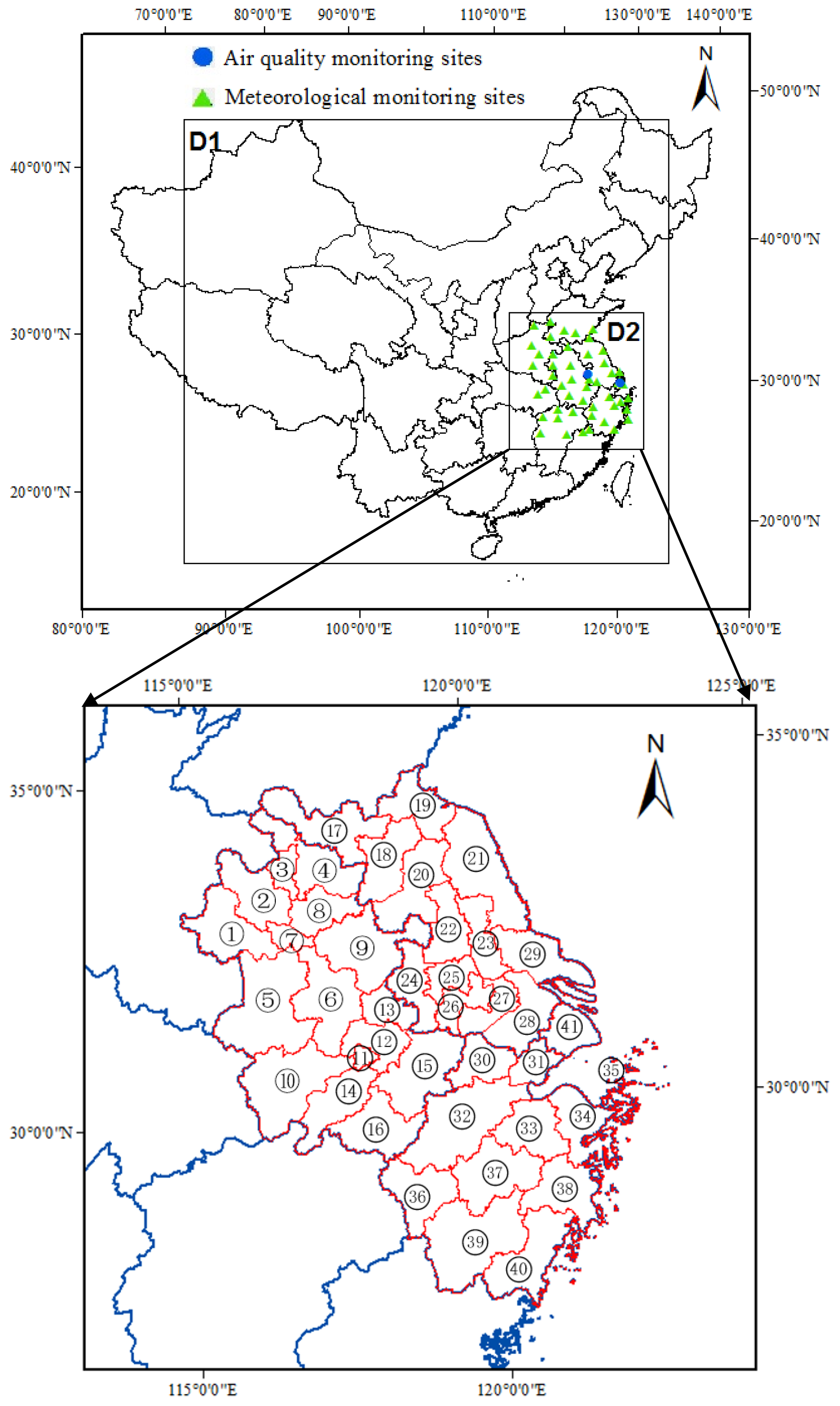
Figure 1Research domain. The blue dots and red triangles indicate the locations of 43 meteorological monitoring sites and 2 air quality monitoring sites, respectively, and the numbers 1–41 represent the prefectural cities of Fuyang, Bozhou, Huaibei, Suzhou, Lu'an, Hefei, Huainan, Bengbu, Chuzhou, Anqing, Tongling, Wuhu, Ma'anshan, Chizhou, Xuancheng, Huangshan, Xuzhou, Suqian, Lianyungang, Huai'an, Yancheng, Yangzhou, Taizhou, Nanjing, Zhenjiang, Changzhou, Wuxi, Suzhou, Nantong, Huzhou, Jiaxing, Hangzhou, Shaoxing, Ningbo, Zhoushan, Quzhou, Jinhua, Taizhou, Lishui, Wenzhou, and Shanghai. The map data provided by Resource and Environment Data Cloud Platform are freely available for academic use (http://www.resdc.cn/data.aspx?DATAID=201, last access: 4 April 2020), © Institute of Geographic Sciences & Natural Resources Research, Chinese Academy of Sciences.
2.1 Emission inventory based on constant emission factors (E1)
The annual NH3 emissions of the YRD region for 2014 were estimated with a bottom-up method based on the constant emission factors and then allocated to the monthly level based on the previously investigated temporal profile of emissions. The inventory contained eight source categories, i.e., fertilizer application, livestock–poultry breeding, fuel combustion, biomass burning, transportation, sewage–waste treatment, industrial processes, and human metabolization (see Table 1 for the details). Note that the emissions from pets were not included in the current work, due to lack of detailed information. Given their relatively small fraction in total emissions, e.g., less than 2 % in the United Kingdom (Sutton et al., 1995, 2000), we believe that the uncertainty was limited. The annual emissions were calculated by prefectural city with Eq. (1):
where E is the emissions (metric tons, t); i and j indicate the prefectural city and source type, respectively; AL is the activity level, which indicates the amount of livestock, the amount of used fertilizer, the fuel burned, or the industrial production, depending on the source type; and EF is the annual emission factor (kg-NH3 per unit of AL).

The activity data were mainly taken or estimated from official statistics at the prefectural city level (if available) or provincial level. For livestock–poultry breeding, the year-end stock and slaughter numbers were used for animals with a breeding cycle respectively more and less than 1 year. If the city-level stock was unavailable, the output of livestock products by prefectural city was applied as the scaling factor to calculate the number from the provincial data. Table S1 in the Supplement summarizes the annual numbers of livestock and poultry by prefectural city in the YRD. The amount of fertilizer used by prefectural city and type was calculated as the product of sown area of cropland and fertilizer rate per unit area of cropland. The sown area by crop type was taken from city-level statistics, and the application rate by fertilizer type was obtained at the provincial level from a national investigation by NDRC (2015). The detailed results of fertilizer activity data are summarized in Table S2. As can also be seen in the table, the aggregated amount of fertilizer used by province was close to the provincial-level statistics, and the deviation relevant to the official statistics was 2.3 % for the whole YRD. The methods and data sources for activity levels of other source categories were provided in our previous studies (Zhou et al., 2017; Zhao et al., 2017; Yang and Zhao, 2019).
The annual NH3 emission factors were obtained based on a thorough literature review and summarized by source category in Table S3. The results from domestic field measurements were preferentially selected. For sources without suitable domestic measurements, the emission factors were also obtained from previous inventories that shared a similar study period as this work. The values from the US and Europe, e.g., AP-42 database (USEPA, 2002) and the EMEP/EEA guidebook (EEA, 2013a, b), were adopted when the above information was lacking.
The monthly distribution of emissions by source was taken from domestic investigations in the YRD (Li, 2012; Zhao et al., 2015; Zhou et al., 2017). For the purpose of air quality modeling, the emissions by sector were allocated into a grid system with a horizontal resolution at 9 km × 9 km based on selected proxies. Those proxies included the distribution of land use (for fertilization), density of total population (for human metabolization and sewage–waste treatment) and rural population (for livestock–poultry breeding and residential solid fuel burning), gross domestic product (for industrial fuel combustion and processes), road network (for transportation), and satellite-derived fire points from the Moderate Resolution Imaging Spectroradiometer (MODIS, for open biomass burning; Davies et al., 2009).
2.2 The method characterizing agricultural processes (E2)
The livestock–poultry breeding emissions were recalculated integrating the detailed regional information of soil, meteorology, and agricultural processes. The same annual activity data as E1 (e.g., livestock–poultry numbers in Table S1 and fertilizer use in Table S2) were applied.
2.2.1 Fertilizer use
The growing seasons of crops affect the temporal distribution of fertilizer use and thereby that of NH3 emissions. We investigated the growing and farming cycles by crop type in the YRD from the regional farming database by the Ministry of Agriculture (MOA, http://202.127.42.157/moazzys/nongshi.aspx, last access: 31 July 2019) and other publications (Zhang et al., 2009). Taking early-season rice as an example, the basal dressing was usually conducted in mid-April, with all the complex fertilizer and half of the other nitrogen fertilizer used. The top dressing was conducted three times, i.e., 10 % and 10 % of nitrogen fertilizer used 7 d and 14 d after transplanting, and the 30 % used for sprouting. With that information incorporated, we estimated the monthly amount of fertilizer usage by prefectural city and fertilizer type based on the annual amount in Table S2.
Emission factors of fertilization were expected to be influenced by soil acidity, temperature, and the fertilization rate. We assumed a linear correlation between the soil pH and NH3 volatilization rate (Huang et al., 2012), and we calculated the monthly emission factors of two fertilization types (basal dressing and top dressing) with Eqs. (2) and (3):
where EFbasal and EFtop are the emission factors for basal dressing and top dressing, respectively; apH and bpH are the slope and intercept depending on soil pH; T0 and kT are the reference temperature and the slope depending on temperature, respectively; Tbasal and Ttop are the monthly average temperature of basal dressing and top dressing, respectively; and CFrate and CFmethod are the correction factors for fertilization rate and application method (basal dressing), respectively.
The spatial distribution of soil pH at a horizontal resolution of 1 km × 1 km was obtained from a world soil database by the International Institute for Applied Systems Analysis (IIASA, http://webarchive.iiasa.ac.at/Research/LUC/External-World-soil-database/HTML/, last access: 4 April 2020). The correlation data between temperature and NH3 volatilization rate were obtained from EEA (2009). Tbasal and Ttop were determined combining the information of farming season by MOA and the daily temperature data from the European Centre for Medium-Range Weather Forecasts (ECMWF, http://apps.ecmwf.int/datasets/data/interim-full-daily/levtype=sfc/#userconsent#, last access: 4 April 2020). All the relevant data for emission factor correction were summarized in Table S4. The monthly NH3 volatilization rates of urea and ammonium bicarbonate (ABC), the two most applied types of fertilizer over the YRD region, are illustrated by season in Fig. S1 in the Supplement. Larger volatilization rates were found in the northern YRD for both fertilizer types, consistent with the distribution of soil pH across the region. Taking urea as an example, the volatilization rates in April and October were commonly smaller than the uniform value applied in E1 at 17.4 %, while those in July were larger. This discrepancy came partly from the consideration of fertilization types in E2. In April and October, basal dressing fertilization was commonly applied at the soil depth of 15–20 cm, restraining the NH3 volatilization. In contrast, the relatively high temperature and top dressing fertilization conducted in July elevated the NH3 volatilization. It should be noted that the local fertilizer application introduced some bias to the soil pH from the global database by IIASA. Basal dressing would increase the soil pH (particularly for acidic soils) as indicated in a previous domestic study (Zhong et al., 2006). Due to a lack of the quantitative relation between the fertilizer application and soil pH at the regional scale in China, we ignored the interaction between them in Eq. (2).
Through the methodology mentioned above, the gridded emission factors and monthly activity levels were obtained to improve the spatial and temporal distributions of NH3 emissions from fertilization. Figure 2 compares the spatial distribution of the monthly fertilizer usage between E1 and E2, indicated by the relative deviation (RD):
In January and July, top dressing fertilization was conducted with limited crop types like rapeseed, corn, and paddy rice, while considerable basal dressing fertilization was investigated in April and October. Inclusion of those details in E2 resulted in smaller estimates of fertilizer use in winter and summer but larger estimates in spring and autumn compared to E1.

Figure 2Differences of fertilizer application between the two inventories in YRD (RD.
2.2.2 Livestock–poultry breeding
In contrast to E1 that calculated the NH3 emissions based on livestock numbers and annual EFs, a mass-flow approach was applied in E2 considering the nitrogen transformation at different stages of manure management (Beusen et al., 2008; EEA, 2013a; Huang et al., 2012). Commonly applied at the global or national scale, the approach calculated NH3 emissions of manure management processes from a pool of total ammoniacal nitrogen (TAN) for three main raising systems, as shown in Fig. S2. In the YRD region, only intensive and free-range systems were considered, and the TAN was calculated by livestock–poultry type based on the breeding duration, the amount and nitrogen contents of urine and feces, and the mass fraction of TAN. The parameters were taken from Yang (2008) and Huang et al. (2012), as summarized in Table S5. According to the nitrogen flow and phase of manure management, the activity levels were then classified into seven categories, including outdoor, housing solid, housing liquid, storage solid, storage liquid, spreading solid, and spreading liquid. NH3 emissions from livestock are calculated as the product of TAN of each category and the corresponding emission factors. As provided in Table S6, the temperature-dependant emission factors by stage and phase were taken from Huang et al. (2012), and the gridded emission factors can then be derived over the YRD region combining the meteorology data from ECMWF.
2.3 Configuration of air quality modeling
The Models-3/Community Multiscale Air Quality (CMAQ) model system version 4.7.1 was applied to evaluate the NH3 emission inventories for the YRD. CMAQ is a three-dimensional Eulerian model designed for understanding the complex interactions of atmospheric chemistry and physics (UNC, 2010). The model has been widely applied and tested in China (Qin et al., 2015; Zhou et al., 2017; Zheng et al., 2019). As shown in Fig. 1, two nested domains were applied with the spatial resolutions of 27 and 9 km, on a Lambert conformal conic projection centered at (34∘ N, 110∘ E). The mother domain (D1, 177×127 cells) covered most parts of China, and the second domain (D2, 118×121 cells) covered the whole YRD region. The two inventories of YRD NH3 emissions developed in this work were applied in D2. Emissions from other pollutants of anthropogenic origin in D1 and D2 outside Jiangsu were obtained from the Multi-resolution Emission Inventory for China (MEIC, http://www.meicmodel.org/, last access: 4 April 2020) with an original spatial resolution of . Population density was applied to relocate MEIC to each modeling domain. A high-resolution inventory that incorporates more information of local emission sources was applied for Jiangsu (JS; Zhou et al., 2017). Both MEIC and JS inventories are for 2012. The emissions for 2014 were obtained using a simple scaling method based mainly on changes in activity levels (e.g., energy consumption and industrial production) between the 3 years. The biogenic emission inventory was from the Model of Emissions of Gases and Aerosols from Nature 2.1 (MEGAN2.1; Guenther et al., 2012; Sindelarova et al., 2014), and the emission inventories of Cl, HCl, and lightning NOx were from the Global Emissions Initiative (GEIA; Price et al., 1997). Meteorological fields were provided by the Weather Research and Forecasting Model (WRF) version 3.4, a state-of-the-art atmospheric modeling system designed for both meteorological research and numerical weather prediction (Skamarock et al., 2008), and the gas-phase Carbon Bond (CB05) mechanism and AERO5 aerosol module were adopted. Other details on model configuration and parameters were given in Zhou et al. (2017). The simulations were conducted for January, April, July, and October to represent the four typical seasons in 2014. A 5 d spin-up period of each month was used to minimize the influences of initial conditions in the simulations.
Using the observation data of the US National Climate Data Center (NCDC) at 43 stations in the YRD (see Fig. 1 for the locations of the stations), the WRF modeling performance was evaluated with statistical indicators including averages of simulations and observations, bias, normalized mean bias (NMB), normalized mean error (NME), root-mean-squared error (RMSE), and index of agreement (IOA). As can be found in Table S7, discrepancies between simulation and observation met the criteria by Emery et al. (2001) for most cases, implying the reliability of meteorological simulation. However, bigger errors were found for the simulation of wind direction.
2.4 Ground-based and satellite observations
There were very limited continuous ground measurement data available for ambient NH3 and aerosol in the YRD region in 2014, particularly at rural–remote sites that are more representative for the regional atmospheric environment. We conducted online hourly measurements using MARGA (Monitor for AeRosols and Gases in ambient Air, ADI2080) at an urban site in the western downtown of Nanjing (32.03∘ N, 118.44∘ E) from August 2014. MARGA is a state-of-the-art instrument which monitors near-real-time water-soluble ions in aerosols and their gaseous precursors (Lanciki, 2018), and it was able to capture rapid compositional changes in PM2.5 (Chen et al., 2017). The site was on the roof of the building of the Jiangsu Provincial Academy of Environmental Science (30 m above the ground) surrounded by residential and commercial buildings and heavy traffic (JSPAES; Li et al., 2015; Chen et al., 2019). The data of October 2014 were applied in this work to evaluate the NH3 inventories through air quality simulation. In addition, the hourly data of online measurement with MARGA were available at a suburban site in Pudong, Shanghai (SHPD), for April, July, and October 2014 (unpublished data from Shanghai Environmental Monitoring Center).
Regarding satellite observation, the daily NH3 vertical column densities (VCDs) measured through the Infrared Atmospheric Sounding Interferometer (IASI) were downloaded from the ESPRI data center (http://cds-espri.ipsl.upmc.fr/etherTypo/index.php?id=1700&L=1, last access: 4 April 2020). We used the data in the domain (26.1–35.4∘ N, 114.2–124.1∘ E) with a 9:30 local time Equator crossing time to evaluate the NH3 emissions. Only pixels with radiative cloud fraction < 25 %, relative error < 100 %, and absolute error < 5×10¹⁵ molec. cm−2 were used following the criteria of previous studies (Van Damme et al., 2014, 2015). The monthly average VCDs for January, April, July, and October 2014 were calculated and allocated into a grid system of 0.5∘ (longitude) ×0.25∘ (latitude) using the Kriging interpolation method, as shown in Fig. 3.

Figure 3The spatial distribution of monthly average of NH3 vertical columns over the YRD region from IASI satellite observation (1015 molec. cm−2).
3.1 Comparison between the two inventories
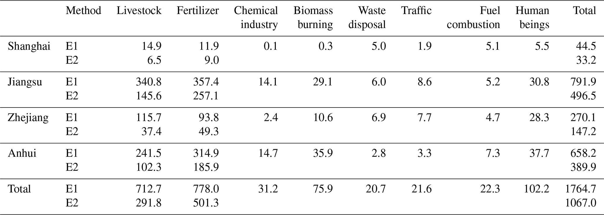
Table 2 summarizes the NH3 emissions estimated with E1 and E2 by source category and province for the YRD region in 2014. Agricultural activities (livestock farming and fertilizer) were identified as the most important sources of NH3, with the fraction of total emissions ranging from 74 % to 84 % in the two methods. Applying the constant emission factors, E1 derived a total NH3 emission estimate 60 % larger than that by E2 that characterized the agricultural processes. In particular, emissions from agricultural activities in E1 were calculated as twice those in E2. At the national scale, similarly, Dong et al. (2010) applied the constant emission factors and estimated the total NH3 emissions to be 16.1 Tg for China, 64 % larger than 9.8 Tg by Huang et al. (2012) with the agricultural processes characterized. The clearly larger estimation by constant emission factors was due partly to the fact that most domestic measurements on the emission factors of NH3 from fertilizer application were conducted in hot seasons (late spring and summer), when the basal dressing of single-season rice and maize and top dressing of wheat were usually conducted (Cai et al., 2002; Huo et al., 2015; Su et al., 2006). However, the crop rotation varied a lot in China, and part of the nitrogen fertilizer was actually not applied in hot seasons. Emission estimation based on those emission factors may thus overestimate the NH3 emission intensity (Huo et al., 2015; Wang et al., 2011; Zhang et al., 2010). Among the provinces, the fraction from Jiangsu of YRD emissions ranged from 45 % to 47 % in the two methods, followed by Anhui with around 37 %. Agricultural activities were relatively intensive in the two provinces: Jiangsu and Anhui contributed 46 % and 33 % of the economic output of agriculture and livestock–poultry farming in the YRD, and the collective fraction of fertilizer use by the two provinces reached 84 %. In contrast, agricultural activities were limited in Shanghai and Zhejiang, with smaller emissions estimated in both inventories.
Table 2Two anthropogenic NH3 emission inventories in the YRD region in 2014 (Gg).
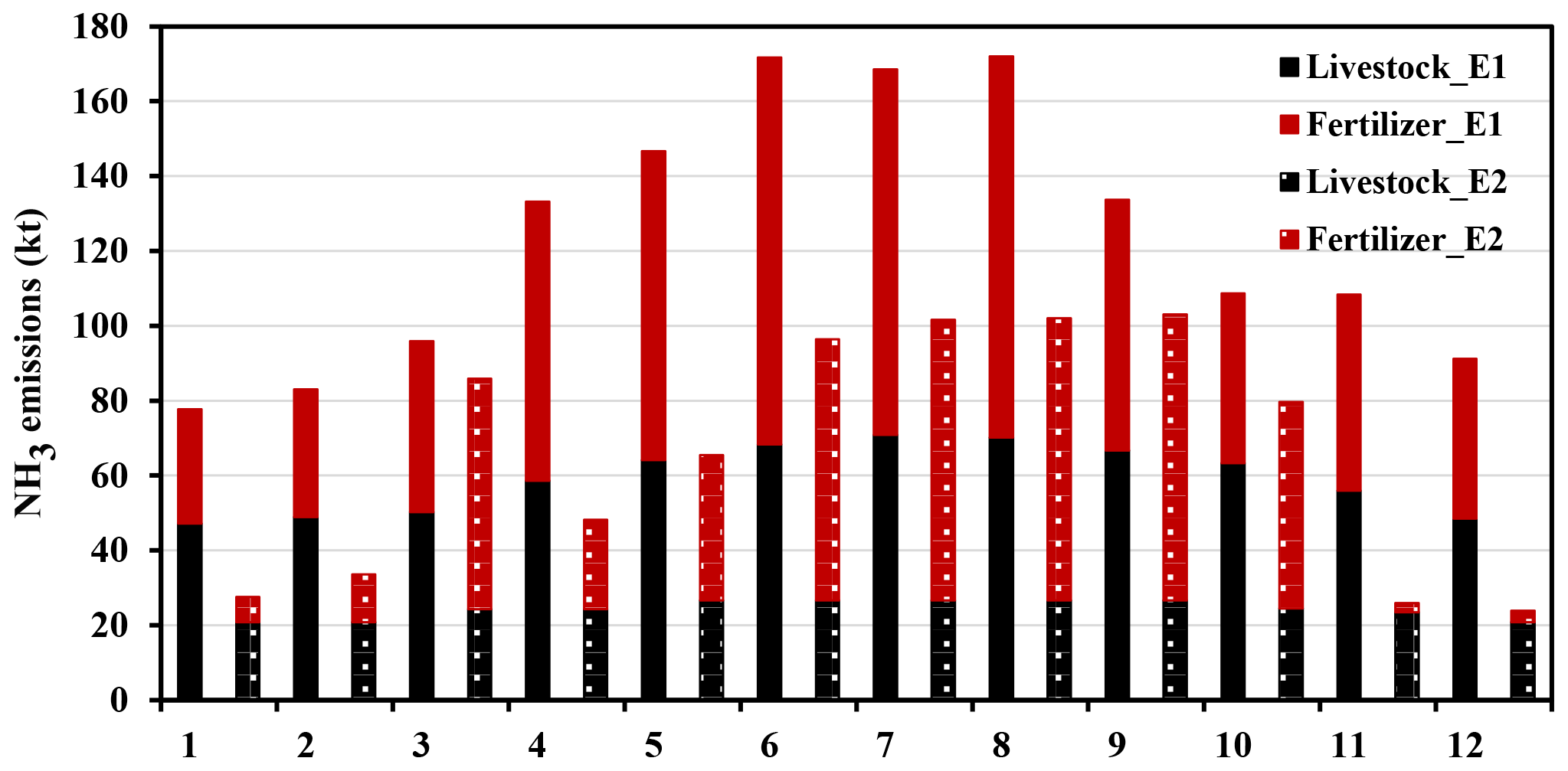
The monthly distribution of NH3 emissions in the two inventories is illustrated in Fig. 4. Both inventories indicated relatively large emissions in summer (from June to August), and elevated emissions were also found in March and September in E2. The difference comes mainly from the effect of farming season on fertilization process. For example, the top dressing fertilization for winter wheat was conducted mostly during the seedling establishment and elongation stage in the following spring, resulting in enhanced use of nitrogen fertilizer in March. Moreover, September was the month with the highest temperature following summer in the YRD in 2014, and the elevated NH3 volatilization led to large emissions in E2. Compared to the fertilizer use, less variation in monthly emissions was found for livestock–poultry breeding, as very limited change in livestock amount was detected in both inventories.
Illustrated in Fig. 5 are the spatial distributions of emissions from fertilizer use, livestock–poultry breeding, and all categories in the two inventories. Both inventories indicated large emission intensities in northern Jiangsu (Xuzhou and Yancheng) and northern Anhui (Fuyang, Bozhou, and Suzhou) with abundant agricultural production. Xuzhou and Yancheng collectively contributed 36 %, 31 %, and 41 % of the provincial fertilizer use, agricultural economic product, and livestock–poultry farming product in Jiangsu, respectively. Similarly, Fuyang, Bozhou, and Suzhou collectively contributed 36 %, 36 %, and 35 % of the provincial sown area, agricultural economic product, and livestock–poultry farming product in Anhui, respectively.
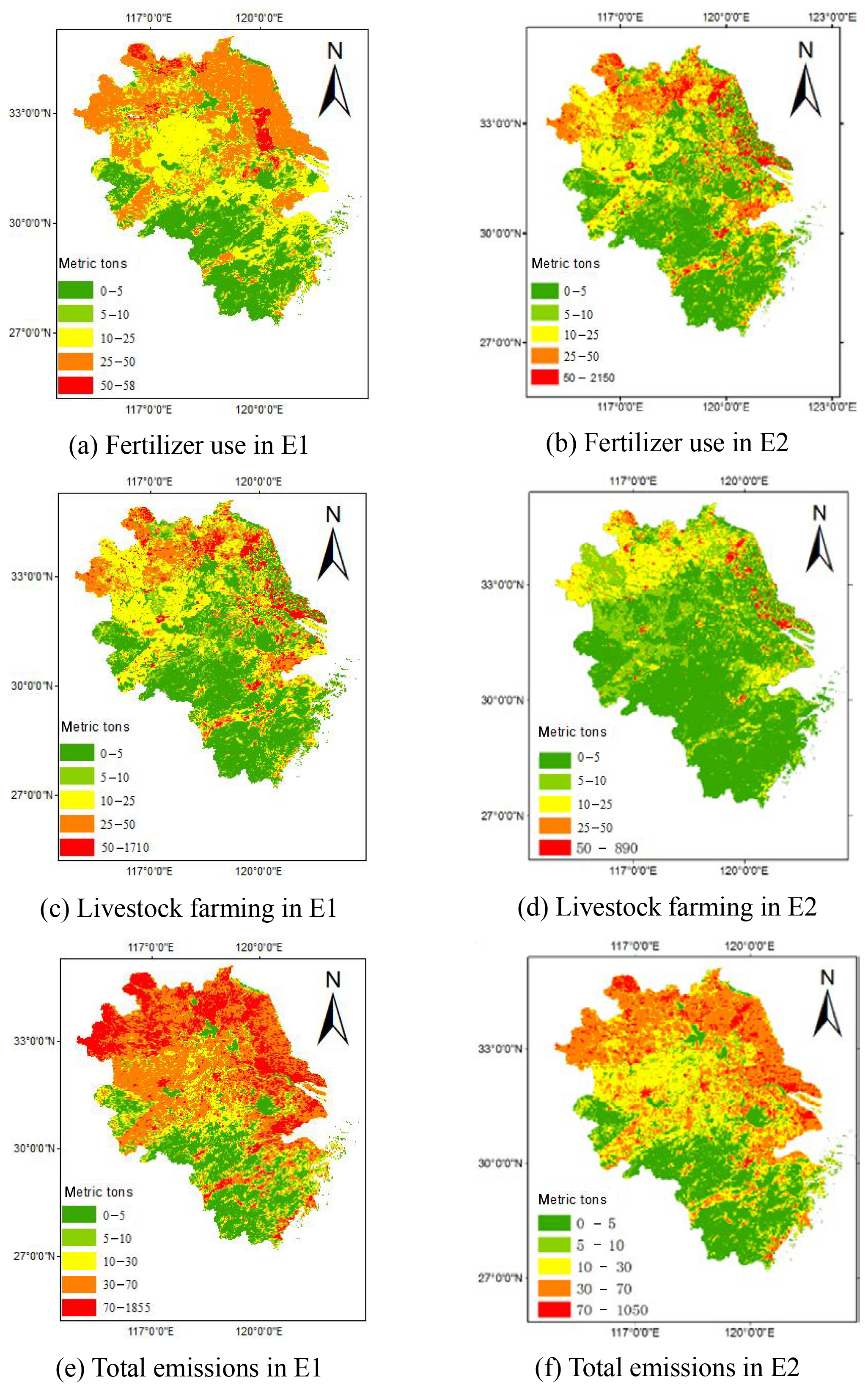
Figure 5Spatial distribution of NH3 emissions from fertilizer use, livestock farming, and all categories in E1 and E2.
The differences in spatial pattern between the two inventories were further investigated for total and fertilizer use emissions by month, through the indicator RD calculated with Eq. (4). As shown in Fig. 6, larger RD was found in northern Jiangsu, northern Anhui, and eastern Zhejiang, while smaller RD was found in western Zhejiang. The emissions in E1 were commonly larger than those in E2 across the YRD region for January and April. In contrast, larger emissions in E2 were found in northern Jiangsu (e.g., Xuzhou and Yancheng) and northern Anhui for July and October. The discrepancy resulted from the combined effect of varied activity data and emission factors as described in Sect. 2.2: top dressing fertilization and high temperature led to enhanced volatilization rate and thereby emissions of NH3 in E2, and the abundant fertilizer use in the cropland in the northern YRD was the main reason for the high emissions in October.

Figure 6Differences of NH3 emissions from fertilizer use and all categories between the two inventories (RD .
Figure 7 compares the NH3 emissions by province and source category in this work and other available downscaled national (MEIC) or provincial inventories in the YRD region. Results from other studies commonly ranged between E1 and E2 for agriculture, the most important NH3 source. With constant emission factors applied, the MEIC estimates were similar to those in E1. Most current provincial inventories made some corrections for emissions from fertilizer use or livestock–poultry breeding, but the local geographical and meteorological information was seldom applied in the emission estimation. For example, Liu and Yao (2016) calculated the emissions from livestock–poultry breeding for Jiangsu based on TAN but did not consider the impacts of varied monthly temperatures on the emissions. Zheng et al. (2016) calculated the agricultural NH3 emissions for Anhui based on a national guideline of NH3 emission inventory development (MEP, 2014) and ignored the impact of soil condition (e.g., pH) on NH3 volatilization from fertilizer use.
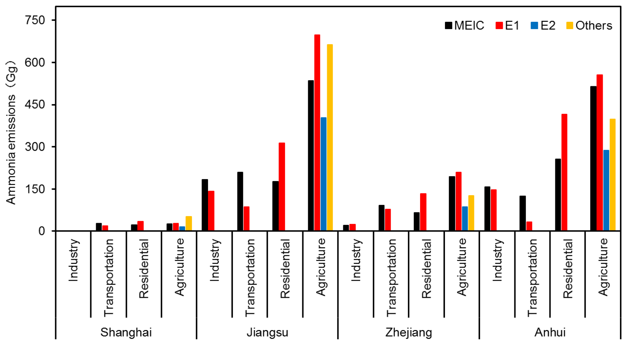
Figure 7Comparison between the estimated NH3 emissions in this work and other studies by province and source category. “Others” indicates Fang et al. (2015), Liu and Yao (2016), Yu et al. (2016), and Zheng et al. (2016) for Shanghai, Jiangsu, Zhejiang, and Anhui, respectively.
3.2 Evaluation of the inventories with transport modeling and ground observations
Figure 8 illustrates the observed and simulated hourly concentrations for gaseous NH3 and inorganic aerosol species (, , and ) in PM2.5 for April, July, and October at SHPD and October at JSPAES. The normalized mean biases (NMBs) and normalized mean errors (NMEs) between observed and simulated concentrations and the monthly average concentrations from observation and simulation are summarized in Table 3. The simulated monthly average concentrations were close to the observed ones at both sites. The biggest discrepancy was found at SHPD for April, where the monthly average NH3 was simulated to be 56 % larger than observations with E1, and the smallest was at JSPAES for October, where the simulation was 1.7 % smaller than observations with E1. The simulated temporal variation, however, was much larger than the observed variation, leading to relatively large NME, particularly at SHPD for April. A clear difference was found for the simulation under two NH3 inventories. In general, the average of simulated NH3 concentrations at the two sites for available months was 27 % smaller in E2 than that in E1 (note the total NH3 emissions in E2 were 38 % smaller than those in E1 for the whole YRD region). At the SHPD site, application of E1 in CMAQ overestimated the NH3 concentration, indicated by the positive NMB values and the larger simulated concentrations than observed concentrations. Such overestimation was corrected when E2 was applied, and the NMEs with E2 were substantially reduced as well, as shown in Table 3. The better modeling performance implies improved estimation and spatiotemporal distribution of emissions. At JSPAES, the air quality modeling with both inventories underestimated the NH3 concentrations, and the simulated monthly average concentration with E1 was much closer to observation than that with E2. The close NMEs between the two inventories indicated very limited improvement at the site, in contrast to SHPD. Located in an urban area, JSPAES might be largely affected by the local sources like transportation and residential activities. NH3 emissions of such source categories, however, were not improved in E2.
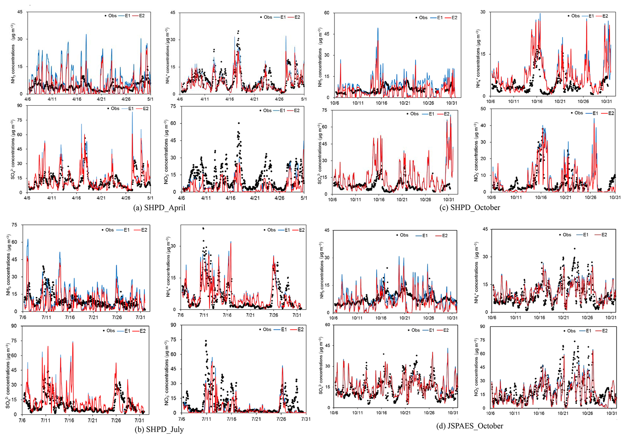
Figure 8The observed and simulated hourly NH3 and SIA concentrations with the two inventories at the JSPAES and SHPD sites.
Table 3Model performance statistics for the hourly concentrations of NH3 and SIA from observation and CMAQ simulation with the two inventories at the SHPD and JSPAES sites for available months.
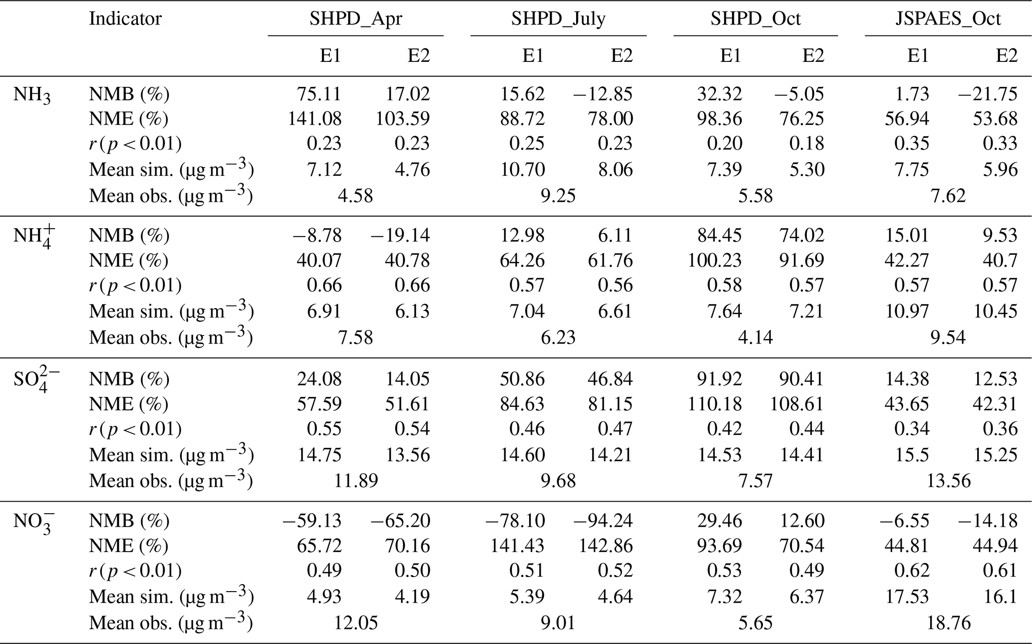
Note: obs. and sim. indicate the results from observation and simulation, respectively. The NMB and NME were calculated using the following equations (P and O indicate the results from modeling prediction and observation, respectively):
To reduce the impact of the highly uncertain hourly meteorology simulation and emission data on air quality modeling, the daily NH3 concentrations derived from simulation and observation were further compared for October at JSPAES. As illustrated in Fig. S3, better agreement between observation and simulation was achieved for the daily concentrations than the hourly concentrations, and the NMEs for E1 and E2 were reduced from 56.9 % and 53.7 % to 37.0 % and 32.5 %, respectively. Besides the emission data, uncertainty in meteorology simulation also contributed to the discrepancy between simulation and observation. For example, both inventories overestimated the concentration on 7 October but underestimated that on 21–22 October. In contrast to the southeasterly wind observed at the ground meteorology station in Nanjing, the simulated wind direction on 7 October was from the north, enhancing the NH3 transport from Yancheng and Xuzhou in northern Jiangsu with intensive agricultural activities. On 21–22 October, the underestimation of NH3 concentration resulted largely from the overestimation in wind speed by WRF.
Compared to NH3, the modeling performance for inorganic aerosols (, , and NO is better for most cases, indicated by the smaller NMEs and larger correlation coefficients (r) in Table 3. Some exceptions exist at SHPD for and in October and in January. Application of E2 reduced the NMEs and improved the simulation of and moderately, but there were no significant changes between the modeling results with E1 and E2. The averages of simulated concentrations at the two sites for available months were 7 %, 3 %, and 12 % smaller in E2 than those in E1 for , , and , respectively, and the differences were clearly smaller than for NH3 at 27 %. As a large fraction of inorganic aerosols come from secondary chemistry reaction, they are more representative for the regional atmosphere condition than the local environment around the measurement site. Therefore, the air quality modeling at a horizontal resolution of 9 km × 9 km is expected to be able to better simulate the concentrations for SIA than the primary gaseous pollutants, particularly when emissions from some local sources are not sufficiently quantified. The simulated concentrations were commonly larger than observations for and , particularly at SHPD in July and October. The uncertainty of the model could be an important source of the discrepancy, as the recent reported mechanisms of gas-to-particle conversion were not sufficiently applied in the CMAQ version we used (Wang et al., 2016; Cheng et al., 2016). In addition, positive or negative artifacts also existed in ground observations with MARGA, resulting from the unexpected reaction between acid gaseous pollutants and nitrate aerosol (Chen et al., 2017; Schaap et al., 2011; Stieger et al., 2018; Wei et al., 2015). From an emissions perspective, the overestimation was partly corrected when smaller NH3 emissions in E2 were applied instead of E1 in the model. Moreover, due to missing information on individual industrial plants, the inventory we used in CMAQ failed to fully capture the progress of emission control in the YRD region and probably overestimated the SO2 emissions (Zhang et al., 2019). The formation of sulfate ammonium aerosols could then be enhanced through the irreversible reaction between SO2 and NH3. The process simultaneously reduced the amount of NH3 reacted with HNO3, further leading to the underestimation of nitrate aerosols. As shown in Table 3, application of E2 with less NH3 emissions than E1 could not improve the modeling performance of nitrate aerosols. The impact of SO2 and NOx emissions on SIA modeling will be further discussed in Sect. 3.4.
3.3 Evaluation of the inventories with transport modeling and satellite observations
To be consistent with the local crossing time of IASI at 09:30 local time, the average of simulated hourly NH3 concentrations at 09:00 and 10:00 local time was applied to calculate the NH3 VCDs, using the following equations:
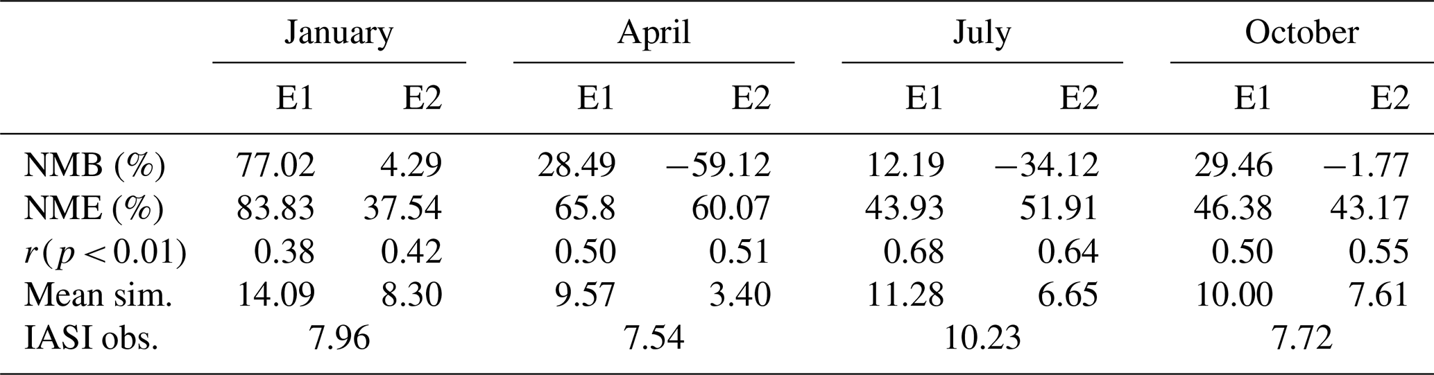
where is the NH3 VCDs from the CMAQ model (molec. cm−2); mk is the simulated NH3 concentrations at the vertical layer k in the CMAQ (molec. cm−3); ΔH is the height of layer k (m); H represents the height when the pressure of atmosphere declines to 1∕e of the original value; and p is the air pressure. Figure 9 illustrates the simulated NH3 VCDs with E1 and E2 for January, April, July, and October. Similar spatial patterns are found with the two inventories; i.e., relatively large NH3 VCDs were simulated mostly in northern Jiangsu and northern Anhui Province, consistent with the hot spot of NH3 emissions. The simulated NH3 VCDs with E1 were 53 % larger than those with E2 across the whole YRD region, with the maximum and minimum monthly differences calculated at 73 % and 31 % for April and October, respectively. The NMB, NME, and correlation coefficient (r) between the observed and simulated VCDs and the monthly average VCDs from observation and simulation are summarized in Table 4. Application of both inventories resulted in larger NH3 VCDs than those from satellite observation for January and October, while the simulated VCDs for April and July were smaller. Besides the uncertainty from monthly distribution of NH3 emissions, the bias from WRF modeling on temperature might also contribute to the discrepancy between simulated and observed VCDs. As shown in Table S7, WRF overestimated the monthly temperature in January and October, with the NMBs calculated at 26.6 % and 0.34 %, and underestimated it in April and July, with the NMBs calculated at −1.62 % and −2.51 %, respectively. Compared to E1, application of E2 significantly reduced the NMEs from 83.8 % to 37.5 % for January and largely corrected the overestimation in VCD simulation for January and October. The simulated VCDs were 4.3 % larger and 1.4 % smaller than observations for the 2 months, respectively. The results implied satisfying agreement between the simulated and observed VCDs over the YRD region. Improvement in NH3 VCD simulation was also found for April when E2 instead of E1 was applied in the air quality modeling, with the NME reduced from 65.8 % to 60.7 %. For July, however, application of E2 did not improve the model performance, implying that the current method in E2 could possibly underestimate the NH3 volatilization when the actual ambient temperature was high. Besides the emissions, the discrepancy could result from various factors including the uncertainty in chemical mechanisms in CMAQ and environmental conditions. Errors from satellite retrieval could also contribute to the inconsistency between simulation and observation. In their study, van Damme et al. (2014), for example, estimated an error of 19 % for the total NH3 columns in Asia. As the ESPRI product of NH3 VCDs we applied in the study does not provide the averaging kernel, however, uncertainty in NH3 column retrieval could result from the reduced sensitivity of satellite measurement towards the surface.
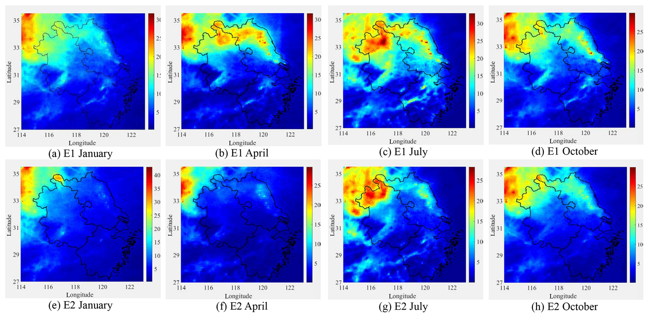
Figure 9The NH3 VCDs in the YRD region simulated with the two inventories by month.
Table 4Model performance statistics for the daily NH3 VCDs from IASI observation and CMAQ simulation using the two inventories by month.
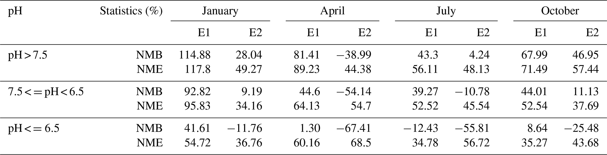
To further investigate the impact of soil pH on the emissions and thereby the modeling performance on NH3 VCDs, the soil in the YRD region was classified to three types, acidic soil (pH ≤6.5), neutral soil (6.5 < pH≤7.5), and alkali soil (pH > 7.5), and the NMBs and NMEs between the simulated and observed NH3 VCDs were calculated by soil type and month, as summarized in Table 5. For neutral and acidic soil, application of E2 that considers the effect of farming season, geophysical condition, and manure management on NH3 emission rates resulted in clearly smaller NMEs than E1, implying the improvement in emission estimation. For acidic soil, however, the NMBs were negative for all the months when E2 was applied, and the NMEs were elevated compared to E1 except for January. Moreover, application of E2 resulted in negative NMBs for neutral and alkali soil in April and July as well. Those results implied that E2 possibly underestimated the NH3 emissions for acidic soil in particular for warm seasons. With the correction of pH and temperature, the NH3 volatilization rate from basal dressing fertilization was relatively low, indicating that the current linear assumption between the soil pH and NH3 volatilization rate might not be appropriate for soil with low pH values for eastern China. As shown in Fig. S4, the measured NH3 volatilization rates from urea and ABC fertilizer use under relatively high soil pH (Zhang et al., 2002; Zhong et al., 2006) were close to the estimated values in E2, but the measured results for acidic soil were clearly larger than those in E2.
Table 5The NMBs and NMEs between the simulated and observed daily NH3 VCDs by soil pH and month.
Limitation should be acknowledged in the emission comparison and evaluation. Besides those we paid extra attention to in E2 (e.g., temperature, soil property, fertilizer application method, and manure management process), other factors could also be influential on air-surface exchange of NH3 and thereby NH3 emissions, including meteorology parameters (wind speed, precipitation, and leaf surface wetness), surface layer turbulence, air and surface heterogeneous-phase chemistry, and plant physiological conditions (Flechard et al., 2013; Gyldenkaerne et al., 2005, Skjøth et al., 2011). With those factors integrated in a bidirectional surface–atmosphere exchange module in air quality modeling, the NH3 emission inventories were improved and the biases in simulation of NH3 and aerosol concentrations were reduced for both the US and Europe (Bash et al., 2013; Wichink Kruit et al., 2012). The fact that we ignored given parameters and processes in the current work could thus partly explain the discrepancy between the simulation and observations. Applying the bidirectional NH3 exchange module, for example, Wichink Kruit et al. (2012) found increased NH3 concentrations for agricultural source areas due to the elevated lifetime and transport distance of NH3 in the model. The result implied a possible correction on the underestimation in NH3 concentrations, as shown in Tables 3 and 4. Therefore, a more comprehensive evaluation and comparison in NH3 emissions is thus suggested for the future, including the bidirectional NH3 exchange and the top-down constraint with inverse modeling.
3.4 Impacts of SO2 and NOx emission estimates on simulated NH3 and aerosols
Besides the meteorology condition, NH3 emissions, and soil pH, the estimates of SO2 and NOx emissions could influence the NH3 and SIA simulation as well. SO2 can be transformed to S (IV) through liquid-phase reaction and then be oxidized to S (VI) by O3, or it can be directly oxidized to H2SO4 by H2O2 or the hydroxyl radical (•OH). HNO3 can be formed through NO2 oxidation by •OH in daytime or through hydrolysis of N2O5 at the aerosol surface at night. Normally NH3 preferentially reacts with H2SO4 and relatively stable (NH4)2SO4 is produced, while NH4NO3 could easily be decomposed under high-temperature or low-humidity conditions. Therefore, the ambient NH3 concentrations and formation of aerosols are influenced by the balance between acidic (SO2 and NOx) and alkaline component (NH3) emissions.
As described in Sect. 2.3, the SO2 and NOx emissions for 2014 used in this work were scaled from those for 2014 based on the changes in activity data. Ignorance of emission control progress during 2012–2014 would probably result in overestimation in emissions. The bias was evaluated through satellite observation. The daily planetary boundary layer (PBL) SO2 and tropospheric NO2 VCDs were obtained from the OMSO2 Level-3 product (http://disc.sci.gsfc.nasa.gov/Aura/data-holdings/OMI/omso2e_v003.shtml, last access: 4 April 2020) and the POMINO Level-3 product from the Ozone Monitoring Instrument (OMI), respectively. As shown in Table S8, all the provinces in the YRD had their SO2 and NO2 VCDs substantially reduced during 2012–2014, and the VCDs declined by 48 % and 31 %, respectively, for the whole region. From a recent unpublished emission study, however, the SO2 and NOx emissions were estimated to decrease by only 16 % and 8 % in the YRD region for the 2 years (personal communication with Cheng Huang from Shanghai Research Academy of Environmental Science, 2019). It can be inferred that the overestimation of SO2 emissions might enhance their reaction with NH3 and thereby the formation of (NH4)2SO4 in the air quality modeling. The formation of , in contrast, might be suppressed accordingly.
3.4.1 Identification of NH3-rich and NH3-poor conditions in the YRD region
To evaluate the nonlinear relation between gaseous pollutant emissions (SO2, NOx, and NH3) and SIA concentrations for the YRD region, we follow Ansari and Pandis (1998) and calculated the gas ratio (GR) based on the modeling results:
where the species in brackets indicate the simulated ambient concentration. A negative GR indicates an NH3-poor condition, and the enhanced NH3 emissions strengthen the oxidation of SO2 and lead to increased (Wang et al., 2011). A GR larger than 1 indicates an NH3-rich condition. Enhanced NH3 emissions have smaller effects on growth of concentrations, and elevated SO2 emissions may accelerate the formation of aerosols, as the increased and reduce the NH4NO3 capacity in the liquid phase. A neutral condition is judged when GR is between 0 and 1.
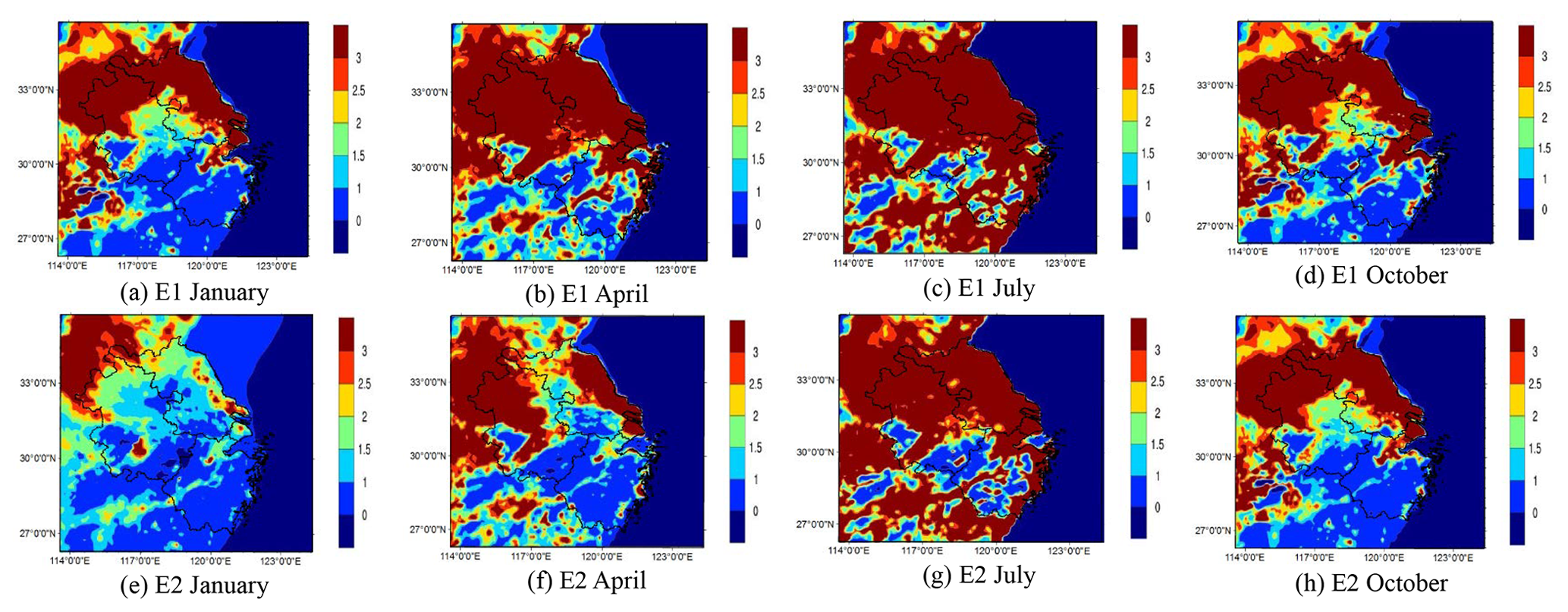
Figure 10The GR values in the YRD region simulated with the two inventories by month.
Figure 10 illustrates the spatial distribution of simulated GR for the YRD region by month with E1 and E2 NH3 inventories. Implied by the GR values larger than 1.0 for most of the areas, the YRD region was identified under the NH3-rich condition when E1 was applied, except for southwest Zhejiang. The judgment is consistent with previous studies (Wang et al., 2011; Dong et al., 2014). With the reduced NH3 emissions in E2, the areas under neutral or NH3-poor conditions expanded in particular for January and April. The common NH3-rich condition suggested potentially high sensitivity of SIA formation to SO2 and NOx emissions.
3.4.2 Sensitivities of NH3 and SIA to SO2 and NOx changes
Three more cases were developed to test the effect of SO2 and NOx emission estimates on NH3 and SIA simulation: Cases 1, 2, and 3 assumed 40 % abatement of SO2 emissions, 40 % abatement of NOx emissions, and 40 % abatement of emissions of both species, respectively. E1 was applied for NH3 emission estimates in all the cases. Table 6 summarizes the modeling performance at JSPAES and SHPD for different cases in October. Clear changes in NH3 and SIA simulation were found with varied SO2 emissions, while the effect of varied NOx emissions on air quality modeling was much smaller. The bias between the simulation and observation was partly corrected for most cases, indicated by the smaller NMBs. Indicated by NMEs, however, the modeling performance was less conclusive. NMEs for and were reduced for Cases 1 and 3, while increased NMEs were found for NH3 and . Limitation in the mechanisms of SIA formation can be an important reason for the discrepancy. Under NH3-rich conditions, abatement of SO2 emissions (Case 1) would reduce the formation of (NH4)2SO4 and thereby lead to growth of NH3 concentrations. This is consistent with the situation in the North China Plain, another region typically suffering from aerosol pollution in China (Liu et al., 2018). The simulated NH3 concentrations were 10.1 % and 11.7 % larger than those in the base case at JSPAES and SHPD, and the simulated SIAs () were 7.9 % and 11.0 % smaller than those in the base case at JSPAES and SHPD, respectively. Based on the modeling results in Table 3, as a comparison, the simulated NH3 concentrations with NH3 emissions in E2 were calculated to be 23 % and 28 % smaller than those with E1 at JSPAES and SHPD for October, respectively, and the analogue number for SIA concentrations was 5 % at both sites. While the estimation of NH3 emissions played an important role on NH3 simulation, the SO2 estimation could be more effective on SIA simulation. Abatement of NOx emissions (Case 2) was much less influential. Less NOx slightly weakened the competition of SIA formation against SO2; thus enhanced formation of (NH4)2SO4 and decreased NH3 concentration were simulated at both sites, as shown in Table 6. When SO2 and NOx were simultaneously reduced in the model (Case 3), similar results were found as with Case 1, implying again that SO2 could be a crucial species in SIA formation in the YRD region. In addition, aerosols were simulated to grow with the 40 % abatement of SO2 and NOx emissions, and the benefits of SO2 and NOx control were partly weakened. To be more effective and efficient in regional air quality improvement, therefore, the control of NH3 emissions should be strengthened along with other pollutants.
Table 6The modeling performance at JSPAES and SHPD in cases with different SO2 and NOx emission estimates. The NMBs and NMEs were based on the observed and simulated hourly concentrations.

We took the YRD region in eastern China as an example and developed two inventories of NH3 emissions for 2014 based on constant emission factors (E1) and those characterizing agricultural processes (E2). Available information from ground and satellite observations was applied to evaluate the inventories through air quality modeling. Both inventories indicated that agricultural activities (livestock farming and fertilizer use) were the most important sources of NH3, but clear differences exist in estimates and spatial and seasonal distribution of NH3 emissions. The total NH3 emissions in E1 were estimated to be 60 % larger than E2, and the emissions from agriculture in E1 were double those in E2. The information on fertilization season and type from local investigation in E2 resulted in discrepancies in monthly distributions of NH3 emissions from E1, particularly in the northern YRD with abundant croplands. Differences in emission estimates lead to varied NH3 concentrations from CMAQ modeling. At the suburban SHPD site, the overestimation in NH3 concentration from CMAQ with E1 could be largely corrected with E2, implying the improved estimation of NH3 emissions by E2. At the urban site JSPAES, however, very limited improvement was achieved when E1 was replaced by E2 in the model, indicating that the emission estimation of local urban sources like transportation and residential activities was not improved in E2. Compared to NH3, the modeling performance for SIA is better for most cases, and differences between the simulated concentrations with E1 and E2 were clearly smaller. Application of E2 improved the simulation of and moderately. For the comparison with the satellite-derived NH3 column, application of E2 significantly corrected the overestimation in VCD simulation for January and October with E1, but it did not improve the model performance for July. Combining the soil distribution, it can be inferred that the current method might underestimate the NH3 volatilization for acidic soil, particularly in warm seasons. Judged by the simulated GR, most of the YRD region was identified as NH3-rich except for southwest Zhejiang. Through the sensitivity test in which SO2 and NOx emissions were solely or simultaneously reduced, estimation of SO2 emissions was detected to be more effective in SIA simulation compared to NH3. Reduced SO2 emissions would suppress the formation of (NH4)2SO4 and thereby lead to growth of NH3 concentrations. The control of NH3 emissions should be strengthened along with that of SO2 and NOx for improving the air quality more effectively and efficiently in the region.
This work is a tentative effort on NH3 emission evaluation at the regional scale. The relations between environmental and meteorology conditions and NH3 volatilization were not fully considered, and the bidirectional surface–atmosphere exchange was not included, resulting in bias in emission estimation. Uncertainties also come from the limitations in ground and satellite observations and the incomplete mechanism of SIA formation in the current air quality model. For better understanding the role of NH3 emissions in regional air quality, more measurements on both sources and ambient concentrations are recommended for the future.
The Multi-resolution Emission Inventory for China used in this study was developed by Tsinghua University (Zheng et al., 2018) and can be obtained at http://www.meicmodel.org/ (MEIC, 2019). The high-resolution inventory for Jiangsu Province was developed by Zhou et al. (2017) and can be accessed at http://www.airqualitynju.com/En/Data/List/Data download (IASI, 2020). The product of daily NH3 VCDs measured through IASI was developed by the research group of Simon Whitburn at Université Libre de Bruxelles and obtained from the ESPRI data center at https://cds-espri.ipsl.upmc.fr/etherTypo/index.php?id=1700&L=1 (JS inventories, 2020). The two NH3 emission inventories developed in this work (E1 and E2) are available online: http://www.airqualitynju.com/En/Data/List/Data download.
The supplement related to this article is available online at: https://doi.org/10.5194/acp-20-4275-2020-supplement.
YZ developed the strategy and methodology of the work and wrote the draft. MY ran the model and produced the figures. XH revised the method and provided useful comments. FC and JZ conducted ground observations of NH3 and aerosols.
The authors declare that they have no conflict of interest.
This article is part of the special issue “Regional assessment of air pollution and climate change over East and Southeast Asia: results from MICS-Asia Phase III”. It is not associated with a conference.
This work was sponsored by the Natural Science Foundation of China (91644220 and 41922052) and the National Key Research and Development Program of China (2017YFC0210106). We would like to acknowledge Qizhen Liu and Zhong Zou from the Shanghai Environmental Monitoring Center and Yunhua Chang from Nanjing University of Information Science & Technology for the ground measurement data, Qiang Zhang from Tsinghua University and Cheng Huang from the Shanghai Research Academy of Environmental Science for emission data, and Simon Whitburn from Université Libre de Bruxelles and Yuanhong Zhao from Peking University for satellite data processing.
This research has been supported by the National Natural Science Foundation of China (grant nos. 91644220 and 41922052) and the National Key Research and Development Program of China (grant no. 2017YFC0210106).
This paper was edited by Joshua Fu and reviewed by three anonymous referees.
Ansari, A. S. and Pandis, S. N.: Response of inorganic PM to precursor concentrations, Environ. Sci. Technol., 32, 2706–2714, 1998.
Bash, J. O., Cooter, E. J., Dennis, R. L., Walker, J. T., and Pleim, J. E.: Evaluation of a regional air-quality model with bidirectional NH3 exchange coupled to an agroecosystem model, Biogeosciences, 10, 1635–1645, https://doi.org/10.5194/bg-10-1635-2013, 2013.
Beusen, A. H. W., Bouwman, A. F., Heuberger, P. S. C., van Drecht, G., and van der Hoek, K. W.: Bottom-up uncertainty estimates of global ammonia emissions from global agricultural production systems, Atmos. Environ., 42, 6067–6077, 2008.
Cai, G. X., Chen, D. L., Ding, H., Pacholski, A., Fan, X. H., and Zhu, Z. L.: Nitrogen losses from fertilizers applied to maize, wheat and rice in the North China Plain, Nutr. Cycl. Agroecosys., 63, 187–195, 2002.
Chen, D., Zhao, Y., Lyu, R., Wu, R., Dai, L., Zhao, Y., Chen, F., Zhang, J., Yu, H., and Guan, M.: Seasonal and spatial variations of optical properties of light absorbing carbon and its influencing factors in a typical polluted city in Yangtze River Delta, China, Atmos. Environ., 199, 45–54, 2019.
Chen, X., Walker, J. T., and Geron, C.: Chromatography related performance of the Monitor for AeRosols and GAses in ambient air (MARGA): laboratory and field-based evaluation, Atmos. Meas. Tech., 10, 3893–3908, https://doi.org/10.5194/amt-10-3893-2017, 2017.
Cheng, Y., Zheng, G., Wei, C., Mu, Q., Zheng, B., Wang, Z., Gao, M., Zhang, Q., He, K., Carmichael, G., Pöschl, U., and Su, H.: Reactive nitrogen chemistry in aerosol water as a source of sulfate during haze events in China, Sci. Adv., 2, e1601530, https://doi.org/10.1126/sciadv.1601530, 2016.
Cheng, Z., Wang, S., Fu, X., Watson, J. G., Jiang, J., Fu, Q., Chen, C., Xu, B., Yu, J., Chow, J. C., and Hao, J.: Impact of biomass burning on haze pollution in the Yangtze River delta, China: a case study in summer 2011, Atmos. Chem. Phys., 14, 4573–4585, https://doi.org/10.5194/acp-14-4573-2014, 2014.
Davies, D. K., Ilavajhala, S., Wong, M. M., and Justice, C. O.: Fire Information for Resource Management System: Archiving and Distributing MODIS Active Fire Data, IEEE T. Geosci. Remote, 47, 72–79, 2009.
Dong, W., Xin, J., and Wang, S.: Temporal and spatial distribution of anthropogenic ammonia emissions in China: 1994–2006, Environ. Sci., 31, 1457–1463, 2010 (in Chinese).
Dong, X., Li, J., Fu, J. S., Gao, Y., Huang, K., and Zhuang, G.: Inorganic aerosols responses to emission changes in Yangtze River Delta, China. Sci. Total Environ., 481, 522–532, 2014.
Emery, C., Tai, E., and Yarwood, G.: Enhanced meteorological modeling and performance evaluation for two Texas episodes, Report to the Texas Natural Resources Conservation Commission, prepared by: ENVIRON, International Corp, Novato, CA, 2001.
European Environment Agency (EEA): EMEP/CORINAIR Air Pollutant Emission Inventory Guidebook-2009, 4.D Crop production and agricultural soils, available at: https://www.eea.europa.eu/publications/emep-eea-emission-inventory-guidebook-2009/part-b-sectoral-guidance-chapters/4-agriculture/4-d/4-d-crop-production-and-agricultural-soils.pdf/view (last access: 25 February 2020), 2009.
European Environment Agency (EEA): EMEP/CORINAIR Air Pollutant Emission Inventory Guidebook-2013, 3.B Manure management, available at: https://www.eea.europa.eu/publications/emep-eea-guidebook-2013/part-b-sectoral-guidance-chapters/4-agriculture/3-b-manure-management/view (last access: 25 February 2020), 2013a.
European Environment Agency (EEA): EMEP/CORINAIR Air Pollutant Emission Inventory Guidebook-2013, 3.D Crop production and agricultural soils, available at: https://www.eea.europa.eu/publications/emep-eea-guidebook-2013/part-b-sectoral-guidance-chapters/4-agriculture/3-d-crop-production/view (last access: 25 February 2020), 2013b.
Fang, X., Shen, G., Xu, C., Qian, X., Li, J., Zhao, Z., Yu, S., and Zhu, K.: Agricultural ammonia emission inventory and its distribution characteristics in Shanghai, Acta Agriculturae Zhejiangensis, 27, 2177–2185, 2015 (in Chinese).
Flechard, C. R., Massad, R.-S., Loubet, B., Personne, E., Simpson, D., Bash, J. O., Cooter, E. J., Nemitz, E., and Sutton, M. A.: Advances in understanding, models and parameterizations of biosphere-atmosphere ammonia exchange, Biogeosciences, 10, 5183–5225, https://doi.org/10.5194/bg-10-5183-2013, 2013.
Fu, X., Wang, S. X., Ran, L. M., Pleim, J. E., Cooter, E., Bash, J. O., Benson, V., and Hao, J. M.: Estimating NH3 emissions from agricultural fertilizer application in China using the bi-directional CMAQ model coupled to an agro-ecosystem model, Atmos. Chem. Phys., 15, 6637–6649, https://doi.org/10.5194/acp-15-6637-2015, 2015.
Fu, X., Wang, S., Xing, J., Zhang, X., Wang, T., and Hao, J.: Increasing ammonia concentrations reduce the effectiveness of particle pollution control achieved via SO2 and NOX emissions reduction in east China, Environ. Sci. Technol. Lett., 4, 221–227, 2017.
Guenther, A. B., Jiang, X., Heald, C. L., Sakulyanontvittaya, T., Duhl, T., Emmons, L. K., and Wang, X.: The Model of Emissions of Gases and Aerosols from Nature version 2.1 (MEGAN2.1): an extended and updated framework for modeling biogenic emissions, Geosci. Model Dev., 5, 1471–1492, https://doi.org/10.5194/gmd-5-1471-2012, 2012.
Guo, H., Cheng, T., Gu, X., Wang, Y., Chen, H., Bao, F., Shi, S. Y., Xu, B. R., Wang, W. N., Zuo, X., Zhang, X. C., and Meng, C.: Assessment of PM2.5 concentrations and exposure throughout China using ground observations, Sci. Total Environ., 1024, 601–602, 2017.
Gyldenkaerne, S., Skjøth, C., Hertel, O., and Ellermann, T. A.: Dynamical ammonia emission parameterization for use in air pollution models, J. Geophys. Res., 110, D07108, https://doi.org/10.1029/2004JD005459, 2005.
Huo, Q., Cai, X., Kang, L., Zhang, H., Song, Y., and Zhu, T.: Estimating ammonia emissions from a winter wheat cropland in North China Plain with field experiments and inverse dispersion modeling, Atmos. Environ., 104, 1–10, 2015.
Huang, R., Zhang, Y., Bozzetti, C., Ho, K., Cao, J., Han, Y., Daellenbach, K. R., Slowik, J. G., Platt, S. M., Canonaco, F., Zotter, P., Wolf, R., Pieber, S. M., Bruns, E. A., Crippa, M., Ciarelli, G., Piazzalunga, A., Schwikowski, M., Abbaszade, G., Schnelle-Kreis, J., Zimmermann, R., An, Z., Szidat, S., Baltensperger, U., EI Haddad, I., and Prevot, A. S. H.: High secondary aerosol contribution to particulate pollution during haze events in China, Nature, 514, 218–222, 2014.
Huang, X., Song, Y., Li, M., Li, J., Huo, Q., Cai, X., Zhu, T., Hu, M., Zhang, H.: A high-resolution ammonia emission inventory in China, Global Biogeochem. Cy., 26, GB1030, https://doi.org/10.1029/2011GB004161, 2012.
IASI: available at: http://www.airqualitynju.com/En/Data/List/Data download, last access: 4 April 2020.
JS inventories: NH3 total column from IASI (Level 2), available at: https://cds-espri.ipsl.upmc.fr/etherTypo/index.php?id=1700&L=1, last access: 4 April 2020.
Kang, Y., Liu, M., Song, Y., Huang, X., Yao, H., Cai, X., Zhang, H., Kang, L., Liu, X., Yan, X., He, H., Zhang, Q., Shao, M., and Zhu, T.: High-resolution ammonia emissions inventories in China from 1980 to 2012, Atmos. Chem. Phys., 16, 2043–2058, https://doi.org/10.5194/acp-16-2043-2016, 2016.
Kurokawa, J., Ohara, T., Morikawa, T., Hanayama, S., Janssens-Maenhout, G., Fukui, T., Kawashima, K., and Akimoto, H.: Emissions of air pollutants and greenhouse gases over Asian regions during 2000–2008: Regional Emission inventory in ASia (REAS) version 2, Atmos. Chem. Phys., 13, 11019–11058, https://doi.org/10.5194/acp-13-11019-2013, 2013.
Lanciki, A.: 2060 MARGA Monitor for AeRosols and Gases in ambient Air. Metrohm Process Analytics, Switzerland, available at: https://www.metrohm.com/en/products/process-analyzers/applikon-marga/ (last access: 10 February 2020), 2018.
Li, B., Zhang, J., Zhao, Y., Yuan, S., Zhao, Q., Shen, G., and Wu, H.: Seasonal variation of urban carbonaceous aerosols in a typical city Nanjing in Yangtze River Delta, China Atmos. Environ., 106, 223–231, 2015.
Li, L.: The numerical simulation of comprehensive air pollution characteristics in a typical city-cluster, PhD thesis, Shanghai University, Shanghai, China, 2012.
Liu, C. and Yao, L.: Agricultural ammonia emission inventory and its distribution characteristics in Jiangsu Province, Journal of Anhui Agricultural Sciences, 44, 70–74, 2016 (in Chinese).
Liu, M., Huang, X., Song, Y., Xu, T., Wang, S., Wu, Z., Hu, M., Zhang, L., Zhang, Q., Pan, Y., Liu, X., and Zhu, T.: Rapid SO2 emission reductions significantly increase tropospheric ammonia concentrations over the North China Plain, Atmos. Chem. Phys., 18, 17933–17943, https://doi.org/10.5194/acp-18-17933-2018, 2018.
Liu, X., Zhang, Y., Han, W., Tang, A., Shen, J., Cui, Z., Vitousek, P., Erisman, J. W., Goulding, K., Christie, P., Fangmeier, A., and Zhang, F.: Enhanced nitrogen deposition over China, Nature, 494, 459–463, 2013.
MEIC: available at: http://www.meicmodel.org/, last access: 31 July 2019.
Ministry of Environmental Protection (MEP): The Guideline of Emission Inventory Development for Atmospheric Ammonia, 2014 (in Chinese).
National Development and Reform Commission of China (NDRC): National data on the cost and profit of agricultural product, China Statistics Press, Beijing, 2015 (in Chinese).
Pan, Y., Tian, S., Zhao, Y., Zhang, L., Zhu, X., Gao, J., Huang, W., Zhou, Y., Song, Y., Zhang, Q., and Wang, Y.: Identifying ammonia hotspots in China using a national observation network, Environ. Sci. Technol., 52, 3926–3934, 2018.
Pan, Y. P., Wang, Y. S., Tang, G. Q., and Wu, D.: Wet and dry deposition of atmospheric nitrogen at ten sites in Northern China, Atmos. Chem. Phys., 12, 6515–6535, https://doi.org/10.5194/acp-12-6515-2012, 2012.
Paulot, F., Fan, S., and Horowitz, L. W.: Contrasting seasonal responses of sulfate aerosols to declining SO2 emissions in the Eastern US: implications for the efficacy of SO2 emission controls, Geophys. Res. Lett., 44, 455–464, https://doi.org/10.1002/2016GL070695, 2017.
Price, C., Penner, J., and Prather, M.: NOX from lightning, Part I: Global distribution based on lightning physics, J. Geophys. Res.-Atmos., 102, 5929–5941, https://doi.org/10.1029/96JD03504, 1997.
Qin, M., Wang, X., Hu, Y., Huang, X., He, L., Zhong, L., Song, Y., Hu, M., and Zhang, Y.: Formation of particulate sulfate and nitrate over the Pearl River Delta in the fall: Diagnostic analysis using the Community Multiscale Air Quality model, Atmos. Environ., 112, 81–89, 2015.
Schaap, M., Otjes, R. P., and Weijers, E. P.: Illustrating the benefit of using hourly monitoring data on secondary inorganic aerosol and its precursors for model evaluation, Atmos. Chem. Phys., 11, 11041–11053, https://doi.org/10.5194/acp-11-11041-2011, 2011.
Sindelarova, K., Granier, C., Bouarar, I., Guenther, A., Tilmes, S., Stavrakou, T., Müller, J.-F., Kuhn, U., Stefani, P., and Knorr, W.: Global data set of biogenic VOC emissions calculated by the MEGAN model over the last 30 years, Atmos. Chem. Phys., 14, 9317–9341, https://doi.org/10.5194/acp-14-9317-2014, 2014.
Skamarock, W. C., Klemp, J. B., Dudhia, J., Gill, D. O., Barker, D. M., Duda, M. G., Huang, X.-Y., Wang, W., and Powers, J. G.: A Description of the Advanced Research WRF Version 3, NCAR Tech. Note NCAR/TN-475+STR, 113 pp., https://doi.org/10.5065/D68S4MVH, 2008.
Skjøth, C. A., Geels, C., Berge, H., Gyldenkærne, S., Fagerli, H., Ellermann, T., Frohn, L. M., Christensen, J., Hansen, K. M., Hansen, K., and Hertel, O.: Spatial and temporal variations in ammonia emissions – a freely accessible model code for Europe, Atmos. Chem. Phys., 11, 5221–5236, https://doi.org/10.5194/acp-11-5221-2011, 2011.
Stieger, B., Spindler, G., Fahlbusch, B. Muller, K., Gruner, A., Poulain, L., Thoni, L., Seitler, E., Wallasch, M., and Herrmann, H.: Measurements of PM10 ions and trace gases with the online system MARGA at the research station Melpitz in Germany – A five-year study, J. Atmos. Chem., 75, 33–70, 2018.
Su, F., Huang, B., Ding, X., Gao, Z., Chen, X., Zhang, F., Kogge, M., and Römheld, V.: Ammonia volatilization of different nitrogen fertilizer types, Soils, 38, 682–686, 2006 (in Chinese).
Sutton, M., Place, C., Eager, M., Fowler, D., and Smith, R.: Assessment of the magnitude of ammonia emissions in the United-Kingdom, Atmos. Environ., 29, 1393–1411, 1995.
Sutton, M. A., Dragosits, U., Tang, Y. S., and Fowler, D.: Ammonia emissions from nonagricultural sources in the UK, Atmos. Environ., 34, 855–869, 2000.
University of North Carolina at Chapel Hill (UNC): Operational Guidance for the Community Multiscale Air Quality (CMAQ) Modeling System Version 4.7.1 (June 2010 Release), available at: http://www.cmaq-model.org (last access: 10 February 2020), 2010.
U.S. Environmental Protection Agency (USEPA): Compilation of Air Pollutant Emission Factors, available at: http://www.epa.gov/ttn/chief/ap42/index.html (last access: 9 March 2019), 2002.
Van Damme, M., Clarisse, L., Heald, C. L., Hurtmans, D., Ngadi, Y., Clerbaux, C., Dolman, A. J., Erisman, J. W., and Coheur, P. F.: Global distributions, time series and error characterization of atmospheric ammonia (NH3) from IASI satellite observations, Atmos. Chem. Phys., 14, 2905–2922, https://doi.org/10.5194/acp-14-2905-2014, 2014.
Van Damme, M., Clarisse, L., Dammers, E., Liu, X., Nowak, J. B., Clerbaux, C., Flechard, C. R., Galy-Lacaux, C., Xu, W., Neuman, J. A., Tang, Y. S., Sutton, M. A., Erisman, J. W., and Coheur, P. F.: Towards validation of ammonia (NH3) measurements from the IASI satellite, Atmos. Meas. Tech., 8, 1575–1591, https://doi.org/10.5194/amt-8-1575-2015, 2015.
Warner, J. X., Dickerson, R. R., Wei, Z., Strow, L. L., Wang, Y., and Liang, Q.: Increased atmospheric ammonia over the world's major agricultural areas detected from space, Geophys. Res. Lett., 44, 2875–2884, https://doi.org/10.1002/2016GL072305, 2017.
Wang, G., Zhang, R., Gomez, M. E., Yang, L., Zamora, M. L., Hu, M., Lin, Y., Peng, J., Guo, S., Meng, J., Li, J., Cheng, C., Hu, T., Ren, Y., Wang, Y., Gao, J., Cao, J., An, Z., Zhou, W., Li, G., Wang, J., Tian, P., Marrero-Ortiz, W., Secrest, J., Du, Z., Zheng, J., Shang, D., Zeng, L., Shao, M., Wang, W., Huang, Y., Wang, Y., Zhu, Y., Li, Y., Hu, J., Pan, B., Cai, L., Cheng, Y., Ji, Y., Zhang, F., Rosenfeld, D., Liss, P. S., Duce, R. A., Kolb, C. E., and Molina, M. J.: Persistent sulfate formation from London Fog to Chinese haze, P. Natl. Acad. Sci. USA, 113, 13630–13635, 2016.
Wang, S., Xing, J., Jang, C., Zhu, Y., Fu, J. S., and Hao, J.: Impact assessment of ammonia emissions on inorganic aerosols in east China using response surface modeling technique, Environ. Sci. Technol., 45, 9293–9300, 2011.
Wei, L., Duan, J., Tan, J., Ma, Y., He, K., Wang, S., Huang, X., and Zhang, Y.: Gas-to-particle conversion of atmospheric ammonia and sampling artifacts of ammonium in spring of Beijing, Science China, 45, 216–226, 2015 (in Chinese).
Wichink Kruit, R. J., Schaap, M., Sauter, F. J., van Zanten, M. C., and van Pul, W. A. J.: Modeling the distribution of ammonia across Europe including bi-directional surface–atmosphere exchange, Biogeosciences, 9, 5261–5277, https://doi.org/10.5194/bg-9-5261-2012, 2012.
Xiao, Z. M., Zhang, Y. F., Hong, S. M., Bi, X. H., Jiao, L., Feng, Y. C., and Wang, Y. Q.: Estimation of the main factors influencing haze, based on a long-term monitoring Campaign in Hangzhou, China, Aerosol Air Qual. Res., 11, 873–882, 2011.
Yang, F., Tan, J., Zhao, Q., Du, Z., He, K., Ma, Y., Duan, F., Chen, G., and Zhao, Q.: Characteristics of PM2.5 speciation in representative megacities and across China, Atmos. Chem. Phys., 11, 5207–5219, https://doi.org/10.5194/acp-11-5207-2011, 2011.
Yang, Y. and Zhao, Y.: Quantification and evaluation of atmospheric pollutant emissions from open biomass burning with multiple methods: a case study for the Yangtze River Delta region, China, Atmos. Chem. Phys., 19, 327–348, https://doi.org/10.5194/acp-19-327-2019, 2019.
Yang, Z.: Estimation of ammonia emission from livestock in China based on mass-flow method and regional comparison, Master thesis, Peking University, Beijing, China, 2008.
Yu, F., Chao, N., Wu, J., Tang, G., Chen, J., Wang, H., and Wu, Z.: Research on agricultural ammonia emission inventory of Zhejiang Province in 2013, Environmental Pollution & Control, 38, 41–46, 2016 (in Chinese).
Zhang, F, Chen, X., and Chen, Q.: The fertilization guideline for the main crop types in China, China Agricultural University Press, Beijing, 2009 (in Chinese).
Zhang, L., Chen, Y., Zhao, Y., Henze, D. K., Zhu, L., Song, Y., Paulot, F., Liu, X., Pan, Y., Lin, Y., and Huang, B.: Agricultural ammonia emissions in China: reconciling bottom-up and top-down estimates, Atmos. Chem. Phys., 18, 339–355, https://doi.org/10.5194/acp-18-339-2018, 2018.
Zhang, Q., Zhang, M., Yang, Y., and Lu, J.: Volatilization of ammonium bicarbonate and urea in main soil of Shandong Province, Chinese J. Soil Sci., 33, 32–34, 2002.
Zhang, X., Wu, Y., Liu, X., Reis, S., Jin, J., Dragosits, U., van Damme, M., Clarisse, L., Whitburn, S., Coheur, P. F., and Gu, B.: Ammonia emissions may be substantially underestimated in China, Environ. Sci. Technol., 51, 12089–12096, 2017.
Zhang, X. Y., Wang, Y. Q., Niu, T., Zhang, X. C., Gong, S. L., Zhang, Y. M., and Sun, J. Y.: Atmospheric aerosol compositions in China: spatial/temporal variability, chemical signature, regional haze distribution and comparisons with global aerosols, Atmos. Chem. Phys., 12, 779–799, https://doi.org/10.5194/acp-12-779-2012, 2012.
Zhang, Y., Dore, A. J., Ma, L., Liu, X., Ma, W., Cape, J. N., and Zhang, F.: Agricultural ammonia emissions inventory and spatial distribution in the North China Plain, Environ. Pollut., 158, 490–501, 2010.
Zhang, Y., Bo, X., Zhao, Y., and Nielsen, C. P.: Benefits of current and future policies on emissions of China's coal-fired power sector indicated by continuous emission monitoring, Environ. Pollut., 251, 415–424, 2019.
Zhao, B., Wang, S, Wang, J., Fu, J. S., Liu, T., Xu, J, Fu, X., and Hao, J.: Impact of national NOx and SO2 control policies on particulate matter pollution in China, Atmos. Environ., 77, 453–463, 2013.
Zhao, Y., Qiu, L. P., Xu, R. Y., Xie, F. J., Zhang, Q., Yu, Y. Y., Nielsen, C. P., Qin, H. X., Wang, H. K., Wu, X. C., Li, W. Q., and Zhang, J.: Advantages of a city-scale emission inventory for urban air quality research and policy: the case of Nanjing, a typical industrial city in the Yangtze River Delta, China, Atmos. Chem. Phys., 15, 12623–12644, https://doi.org/10.5194/acp-15-12623-2015, 2015.
Zhao, Y., Mao, P., Zhou, Y., Yang, Y., Zhang, J., Wang, S., Dong, Y., Xie, F., Yu, Y., and Li, W.: Improved provincial emission inventory and speciation profiles of anthropogenic non-methane volatile organic compounds: a case study for Jiangsu, China, Atmos. Chem. Phys., 17, 7733–7756, https://doi.org/10.5194/acp-17-7733-2017, 2017.
Zheng, H., Cai, S., Wang, S., Zhao, B., Chang, X., and Hao, J.: Development of a unit-based industrial emission inventory in the Beijing–Tianjin–Hebei region and resulting improvement in air quality modeling, Atmos. Chem. Phys., 19, 3447–3462, https://doi.org/10.5194/acp-19-3447-2019, 2019.
Zheng, Z., Weng, J., Wang, S., and Wang, J.: Estimation of ammonia emission in Anhui Province, Journal of Anhui Agricultural Sciences, 8, 73–75, 2016 (in Chinese).
Zheng, B., Tong, D., Li, M., Liu, F., Hong, C., Geng, G., Li, H., Li, X., Peng, L., Qi, J., Yan, L., Zhang, Y., Zhao, H., Zheng, Y., He, K., and Zhang, Q.: Trends in China's anthropogenic emissions since 2010 as the consequence of clean air actions, Atmos. Chem. Phys., 18, 14095–14111, https://doi.org/10.5194/acp-18-14095-2018, 2018.
Zhong, N., Zeng, Q., Zhang, L., Liao, B., Zhou, X., and Jiang, J.: Effects of acidity and alkalinity on urea transformation in soil, Chinese J. Soil Sci., 37, 1123–1128, 2006 (in Chinese).
Zhou, Y., Zhao, Y., Mao, P., Zhang, Q., Zhang, J., Qiu, L., and Yang, Y.: Development of a high-resolution emission inventory and its evaluation and application through air quality modeling for Jiangsu Province, China, Atmos. Chem. Phys., 17, 211–233, https://doi.org/10.5194/acp-17-211-2017, 2017.