the Creative Commons Attribution 4.0 License.
the Creative Commons Attribution 4.0 License.
 | 31 Mar 2020
Ozone–vegetation feedback through dry deposition and isoprene emissions in a global chemistry–carbon–climate model
Cheng Gong
Yadong Lei
Yimian Ma
Hong Liao
Ozone–vegetation feedback is essential to tropospheric ozone (O3) concentrations. The O3 stomatal uptake damages leaf photosynthesis and stomatal conductance and, in turn, influences O3 dry deposition. Further, O3 directly influences isoprene emissions, an important precursor of O3. The effects of O3 on vegetation further alter local meteorological fields and indirectly influence O3 concentrations. In this study, we apply a fully coupled chemistry–carbon–climate global model (ModelE2-YIBs) to evaluate changes in O3 concentrations caused by O3–vegetation interactions. Different parameterizations and sensitivities of the effect of O3 damage on photosynthesis, stomatal conductance, and isoprene emissions (IPE) are implemented in the model. The results show that O3-induced inhibition of stomatal conductance increases surface O3 on average by +2.1 ppbv (+1.2 ppbv) in eastern China, +1.8 ppbv (−0.3 ppbv) in the eastern US, and +1.3 ppbv (+1.0 ppbv) in western Europe at high (low) damage sensitivity. Such positive feedback is dominated by reduced O3 dry deposition in addition to the increased temperature and decreased relative humidity from weakened transpiration. Including the effect of O3 damage on IPE slightly reduces surface O3 concentrations by influencing precursors. However, the reduced IPE weaken surface shortwave radiative forcing of secondary organic aerosols, leading to increased temperature and O3 concentrations in the eastern US. This study highlights the importance of interactions between O3 and vegetation with regard to O3 concentrations and the resultant air quality.
- Article
(8937 KB) -
Supplement
(3057 KB) - BibTeX
- EndNote


Tropospheric ozone (O3) is generated by photochemical reactions involving nitrogen oxides (NOx) and volatile organic compounds (VOCs) under strong solar radiation (Sillman, 1999; Atkinson, 2000; Jacob and Winner, 2009). It is one of the most important air pollutants and has been of widespread concern (Wang et al., 2017; Li et al., 2019). High O3 concentrations at the surface can not only injure human respiratory health (Gauderman et al., 2004; Lelieveld et al., 2015) but also lead to considerable damage to plants and crops, which further changes the land carbon budget (Fuhrer et al., 1997; Yue and Unger, 2014; Lombardozzi et al., 2015). In turn, vegetation can modulate O3 concentrations via influencing dry deposition processes, precursor emissions (such as those of isoprene, monoterpene, and sesquiterpene), and meteorological fields. Studying O3–vegetation interactions is of great importance to better understand the variations in O3 concentrations as well as the ecosystem carbon cycle, particularly for regions with high O3 levels and vegetative cover.
Ground-level O3 reduces vegetation photosynthesis by stomatal uptake (Fuhrer et al., 1997; Ainsworth et al., 2012). Through a globally statistical meta-analysis, Wittig et al. (2007) showed that the elevated O3 since the preindustrial period depressed photosynthesis and stomatal conductance of trees by 9 %–13 % and 11 %–15 %, respectively. A recent global meta-analysis on poplar showed that current O3 concentrations reduced the CO2 assimilation rate and stomatal conductance by 33 % and 25 %, respectively, compared to that of charcoal-filtered air (Feng et al., 2019a). In model studies, an offline process-based vegetation model (the Yale Interactive Terrestrial Biosphere model, or YIBs) estimated that the present-day effect of O3 damage reduced gross primary productivity (GPP) by 4 %–8 % on average over the eastern US during the summer (Yue and Unger, 2014) and annual net primary productivity (NPP) by approximately 14 % in China (Yue et al., 2017). Lombardozzi et al. (2015) also showed that the present-day O3 exposure reduces GPP globally by 8 %–12 % using the Community Land Model (CLM).
Isoprene emissions (IPE) from vegetation can be affected by surface O3. Isoprene is the most dominant species among biogenic VOCs (BVOCs) and accounts for approximately one-half of global BVOC emissions (Guenther et al., 2012). The effect of O3 on IPE is complex. Calfapietra et al. (2009) reviewed observational experiments in Italy and proposed a hypothesis that there might be a detoxification effect resulting from O3–IPE interactions. Vegetation under a low accumulated O3 dose can be simulated to increase the levels of IPE to reduce oxidative damage, but months of O3 exposure are harmful to metabolism and reduce IPE. Several studies have showed that O3 fumigation over a short time (days to weeks) but at high concentrations (100–300 ppbv) led to increased IPE (Velikova et al., 2005; Fares et al., 2010), while some other experiments conducted over an entire growing season (at least 3 months) under controlled O3 concentrations (approximately 80 ppbv) showed that O3 reduced IPE (Calfapietra et al., 2008; Yuan et al., 2016, 2017). A recent global meta-analytic review showed that IPE negatively responded to elevated O3 (91 ppbv on average) by −8 % (Feng et al., 2019b). Overall, consecutive exposure to high O3 levels has a negative impact on IPE, although there are large uncertainties resulting from vegetation type (Tiiva et al., 2007; Ryan et al., 2009), temperature (Hartikainen et al., 2009), and CO2 concentration (Calfapietra et al., 2008).
O3 dry deposition is one of the important sinks of tropospheric O3 and mainly occurs over vegetation (Wesely, 1989). The stomatal uptake of vegetation plays an important role in this removal process. (Wesely and Hicks, 2000). Val Martin et al. (2014) showed that the O3 dry deposition velocity in the Community Earth System Model (CESM) significantly increased and was more reasonable when the original scheme (Wesely, 1989), which assumed that stomatal resistance was only related to temperature and water vapor, was replaced with a scheme coupled to vegetation (Collatz et al., 1991; Sellers et al., 1996). In addition, BVOC emissions can change the local NOx∕VOC ratio and, in turn, influence O3 concentrations. For example, Fu and Liao (2012) showed that the interannual variations in BVOCs alone can lead to 2 %–5 % differences in simulated O3 over China during the summer using the Model of Emissions of Gases and Aerosols from Nature (MEGAN; Guenther et al., 2006) module embedded within the global three-dimensional chemical transport model (GEOS-Chem). Calfapietra et al. (2013) reviewed the role of BVOCs emitted by urban trees in O3 concentrations in cities and showed that BVOCs generally promoted O3 formation because of the VOC-limited condition. Furthermore, the modifications of meteorological fields caused by vegetation (Liu et al., 2006; Wu et al., 2011) may also potentially have an effect on O3 formation as well as vegetation growth. As a result, O3 stomatal uptake (O3 dry deposition via stomata), BVOC emissions, and changes in meteorological fields are connected and jointly affect O3 concentrations.
Thus far, very few studies have comprehensively investigated the O3–vegetation feedback at a global scale. Sadiq et al. (2017) investigated the effect of O3 damage on the photosynthesis rate and stomatal conductance as well as potential meteorological feedback on surface O3 concentrations using the CESM. They found that O3–vegetation interactions led to increased O3 concentrations mainly in Europe, the northern US, and northern China. However, the effect of O3 on BVOCs was not directly considered but was indirectly simulated by the increased temperature resulting from O3–vegetation interactions. The O3 damage sensitivities for photosynthesis and stomatal conductance were calculated by using two decoupled linear regressions with accumulated O3 concentrations. However, the linear slope of the photosynthetic rate and stomatal conductance to O3 was zero for some vegetation types (such as broadleaf forests), showing the significant effect of O3 damage even at zero O3 concentrations. Based on the same flawed O3 damage scheme, Zhou et al. (2018) calculated responses of the leaf area index (LAI) to surface O3 and implemented steady-state results for the GEOS-Chem model to simulate O3 perturbations. Such asynchronous coupling may underestimate O3 changes caused by the full pollution–biosphere interactions, not to mention the omission of feedback of O3 to BVOC emissions and meteorology. More comprehensive work utilizing a validated O3 damage scheme and considering the direct effect of O3 on BVOCs is necessary to reasonably predict O3–vegetation feedback on O3 concentrations.
In this study, we apply a semi-mechanistic O3 damage scheme (Sitch et al., 2007) to the YIBs dynamic vegetation model coupled with the global Earth system model NASA ModelE2 (ModelE2-YIBs) to explore O3-induced changes in stomatal conductance and evaluate the consequences of such changes on surface O3 concentrations (O3–vegetation feedback via O3 dry deposition). Then, two schemes are proposed to estimate the contributions of O3 damage to IPE based on the existing scheme generated by Sitch et al. (2007), and observations are made. The feedback of O3 damage to both stomatal conductance and IPE and the resultant effect on surface O3 concentrations is calculated by using ModelE2-YIBs. Finally, the associated meteorological feedback to O3 concentrations is discussed. We found that the O3–vegetation feedback enhanced surface O3 concentrations particularly in O3-polluted regions.
2.1 The NASA ModelE2-YIBs model
NASA ModelE2-YIBs is a fully coupled chemistry–carbon–climate global model with a horizontal resolution of 2∘ latitude × 2.5∘ longitude and 40 vertical layers up to 0.1 hPa. The dynamic and physical processes are calculated every 30 min. Gas-phase chemistry in the troposphere includes basic NOx–HOx–Ox–CO–CH4 chemistry as well as peroxyacyl nitrates and the following hydrocarbons: terpenes, isoprene, alkyl nitrates, aldehydes, alkenes, and paraffins. Chlorine-containing and bromine-containing compounds, chlorofluorocarbons (CFCs), and N2O source gases are all included in the stratospheric gas-phase chemistry. Dry deposition of gases is calculated by using a resistance-in-series scheme, which was updated to include coupling to stomatal resistance (Val Martin et al., 2014). In addition, the model interactively simulates aerosols such as sulfate, nitrate, elemental and organic carbon, sea salt, and dust considering the climate through direct (Koch et al., 2006) and indirect effects (Menon et al., 2008, 2010) and gas-phase chemistry by affecting photolysis rates (Bian et al., 2003). Meteorological and hydrological variables in this model have been fully validated via observations and a reanalysis dataset (Schmidt et al., 2014). The anthropogenic emission inventory for the present-day (2010) from the IPCC RCP8.5 scenario (van Vuuren et al., 2011) is utilized in this study.
The YIBs model is a dynamic vegetation model that includes nine plant functional types (PFTs; Table S1 in the Supplement) and can simulate biophysical processes of photosynthesis, transpiration, and respiration with variations in meteorological fields. Since the higher leaf photosynthesis requires larger stomatal conductance to allow more CO2 enter the leaves, leaf photosynthesis and stomatal conductance are closely related and calculated using the Farquhar and Ball–Berry models (Farquhar et al., 1980; Ball et al., 1987) as follows:
where the total leaf photosynthesis (Atot) is the minimum value of the ribulose-1,5-bisphosphate carboxylase-limited (RuBisCO-limited) rate of carboxylation (Jc), light-limited rate (Je), and export-limited rate (Js). Stomatal conductance for H2O (gs) is calculated by the Atot, dark respiration rate (Rd), relative humidity (RH), and CO2 concentration at the leaf surface (cs). The values of m and b are different for different PFTs (Table S1). A canopy radiation scheme is applied in YIBs to separate diffuse and direct light for sunlit and shaded leaves (Spitters et al., 1986). The LAI and tree growth are dynamically simulated with the allocation of carbon assimilation. The emissions of isoprene are calculated online as a function of Je photosynthesis (Eq. 1), canopy temperature, intercellular CO2, and CO2 compensation point (Arneth et al., 2007; Unger, 2013) and have been fully validated by Unger et al. (2013). Carbon fluxes, phenology, LAI, GPP, and net ecosystem exchange (NEE), as well as other parameters of vegetation in ModelE2-YIBs, have been previously extensively evaluated and agree well with the observations (Yue and Unger, 2015). In addition, ModelE2-YIBs shows good performance in simulating O3–vegetation interactions such as O3–GPP and O3–gs relationships (Yue et al., 2016; Yue et al., 2018).
The O3 dry deposition velocity (Vd) in ModelE2-YIBs is calculated following the multiple-resistance approach originally described by Wesely (1989):
where Ra, Rb, and Rc are the aerodynamic resistance, quasi-laminar sublayer resistance above the canopy, and surface resistance, respectively. Rc is computed as follows:
where Rs, Rlu, Rcl, and Rg represent the stomatal resistance, leaf cuticle resistance, lower-canopy resistance, and the ground resistance, respectively. In this study, the original parameterization for Rs, which is empirically expressed by solar radiation, surface air temperature, and the molecular diffusivities for water vapor, has been substituted by the reciprocal of gs from Eq. (2) following Val Martin et al. (2014). In this case, O3 dry deposition can be interactively influenced by the stomatal O3 uptake process for vegetation.
Isoprene and α-pinene are considered to be the precursors for biogenic secondary organic aerosols (SOAs) in ModelE2-YIBs, which are computed online based on the two-product scheme developed by Chung and Seinfeld (2002). Isoprene can be oxidized by O3 as follows:
Changes for semivolatile product Pi () at each time step (dt) are calculated by
where rr is the chemical reaction rate of O3 and isoprene calculated by the Arrhenius equation. [O3] and [C5H8] are the O3 and isoprene concentrations, respectively. Ai is the molar-based stoichiometric coefficient depending on SOA formation pathways (high or low NOx; Lane et al., 2008). Temperature (T) dependence on the partitioning coefficient (Kp) is given by the Clausius–Clapeyron equation:
where ΔH is the enthalpy of vaporization and is set as 42.0 kJ mol−1 for isoprene (Chung and Seinfeld, 2002; Henze and Seinfeld, 2006) and 72.9 kJ mol−1 for α-pinene. Ksc is the saturation concentrations at the temperature Tsc (295 K) and set as 1.62 m3 µg−1 (0.064 m3 µg−1)and 0.0086 m3 µg−1 (0.0026 m3 µg−1) for the two products formed by oxidation of isoprene (α-pinene), respectively (Presto et al., 2005; Henze and Seinfeld, 2006).
2.2 Schemes describing the effect of O3 damage to vegetation
2.2.1 The effect of O3 damage to photosynthesis and stomatal conductance
A semi-mechanistic scheme proposed by Sitch et al. (2007) is applied in this study that simulates the effect of O3 damage to the photosynthesis rate via the following formula:
where Atotd (gsd) and Atot (gs) are the O3-affected and original total leaf photosynthesis (stomatal conductance), respectively. F is the ratio between affected and original photosynthesis. It depends on the instantaneous leaf uptake of O3 as follows:
where parameter a represents the O3-damaging sensitivity dependent on vegetation types with a range from low to high values. is a critical threshold for damage (Table S1). is the O3 uptake rate by the stomata, which is calculated by
where [O3] is the surface O3 concentrations and Ra is the aerodynamic resistance in Eq. (3). is 1.67, which is the ratio of leaf resistance for O3 to leaf resistance for water vapor. This scheme has been utilized in many previous studies, which have reported that O3 reduces GPP by 4 %–8 % on an annual mean basis in the eastern US and by 10 %–20 % during the summer in China (Yue and Unger, 2014; Yue et al., 2017).
2.2.2 The effect of O3 damage to IPE
To date, there are no mature parameterizations that calculate the contributions of O3 damage to IPE. Here, we propose two schemes based on observations to quantify the changes in surface O3 concentrations resulting from O3 damage to IPE.
The first scheme assumes that O3 leads to the same percentage of damage to photosynthesis and IPE because IPE are observed to linearly vary with photosynthesis (Yuan et al., 2016). The affected IPE (IPEd) can be calculated as follows:
where F is calculated by using Eq. (10) and IPE is the original level of IPE. Hereafter, this scheme is termed the “F scheme”.
Another scheme is based on open-top chamber (OTC) observations. Although many experiments have studied the effects of O3 on IPE, most have applied a limited range of O3 levels (e.g., 7.3–56.6 ppbv in Hartikainen et al., 2009, or > 100 ppbv in Fares et al., 2010). In reality, surface O3 concentrations can vary from several parts per billion by volume (e.g., in the polar region during the winter) to over 100 ppbv (e.g., in megacities of China during the summer). To date, only one study (Yuan et al., 2017) has explored the responses of IPE to different levels of O3 damage for two poplar clones; a linear regression between the percentage damage of IPE (PDI) and the cumulative stomatal uptake of (POD1) was derived as follows:
The POD1 is calculated by the following formula:
where is the O3 uptake rate by stomata (nmol O3 ), which is the same as that in Eq. (11). dt indicates the time integration step, and n indicates the total number of time steps during the growing season. In this study, the POD1 accumulated over the growth season is defined as April to October north of 23.5∘ N (e.g., Tucker et al., 2001; White et al., 2002; Yin et al., 2014; Wang et al., 2019), November to March south of 23.5∘ S (e.g., Broich et al., 2015; Moore et al., 2016), and 200 d between 23.5∘ N and 23.5∘ S because the leaf phenology in tropical evergreen forests is not determined by seasonality (Xiao et al., 2006). Limited by the data availability, we apply the PDI function (Eq. 13) for poplar to all vegetation types as follows:
Hereafter, this scheme is termed a “linear scheme.” Different from the F scheme, the linear scheme calculates IPE damage using accumulated O3 instead of instantaneous O3 concentrations.
2.3 Descriptions for sensitivity experiments
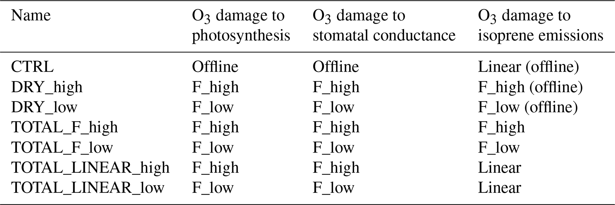
Seven experiments (Table 1) are conducted to explore the feedback of vegetation on surface O3 concentrations via influencing O3 dry deposition, IPE, and meteorological fields. The control simulation (CTRL) does not include the effect of O3 damage to vegetation. Two cases (DRY_high and DRY_low) are established to investigate the feedback via O3 dry deposition with high or low O3 damage sensitivities (a in Eq. 10). Then, the effect of O3 damage to IPE is added by using either F or linear schemes, resulting in four more experiments (TOTAL_F_high, TOTAL_F_low, TOTAL_LINEAR_high, and TOTAL_LINEAR_low). In the CTRL run, the effects of O3 damage to photosynthesis, stomatal conductance, and IPE (the linear scheme) are calculated offline; such damages are not fed back to affect vegetation growth and dry deposition of O3. The offline O3 damage to IPE produced by using the F scheme is calculated in DYR_high and DYR_low.
For each experiment, 20-year simulations are performed with five initial spin-up years. Outputs of the last 15 years are averaged and analyzed. Regionally, the results in the eastern US (30–45∘ N, 75–90∘ W), western Europe (35–60∘ N, 10∘ W–20∘ E), and eastern China (20–40∘ N, 105–122∘ E) are compared and discussed.
2.4 Observed ground-level O3 network and model evaluation
To evaluate simulated O3 concentrations, three observational networks are utilized as follows: the Air Quality Monitoring Network from the Ministry of Ecology and Environment (AQMN-MEE) in China, Clean Air Status and Trends Network (CASTNET) in the US, and European Monitoring and Evaluation Programme (EMEP) in Europe. The summer concentrations for CASTNET and EMEP are averaged over the year 2010, but those for AQMN-MEE are averaged over 2014 because this network was established in 2013 and started to provide high-quality data beginning in 2014. The simulated O3 concentrations are interpolated in the observational sites by using a bilinear interpolation method. Normalized mean biases (NMBs) are calculated by using the following equation:
where Si and Oi are the simulated and observed O3 concentrations, respectively, and n is the total number of observational sites.
3.1 CTRL simulation and model evaluation
Figure 1 shows a comparison of the simulated summer O3 concentrations to the observations. The model reasonably reproduces spatial patterns, with a correlation coefficient of 0.41. The NMBs between simulations and observations in US and Europe are 11.7 % and 13.2 %, respectively, which are comparable with the simulation performed by CESM (Lamarque et al., 2012; Sadiq et al., 2017). However, the model overestimates O3 concentrations by 29.3 % with a regression intercept of 32 ppbv, suggesting that simulated O3 vegetation damage might be overestimated especially over some regions with a low ambient O3 level. The large overestimate is mainly a result of overestimation in China. However, if we validate maximum daily 8 h average (MDA8) O3 concentrations, we found that the model shows much lower biases (Fig. S1 in the Supplement). The main reason for the overestimation is that the model predicts high nighttime O3 concentrations that are not consistent with observations. Since O3–vegetation interactions usually occur in the daytime, the validation shows that ModelE2-YIBs is good to use for this study. Meanwhile, most of the observational sites in AQMN-MEE are located in urban areas, which might be another reason for the surface O3 overestimates in China (Yue et al., 2017).
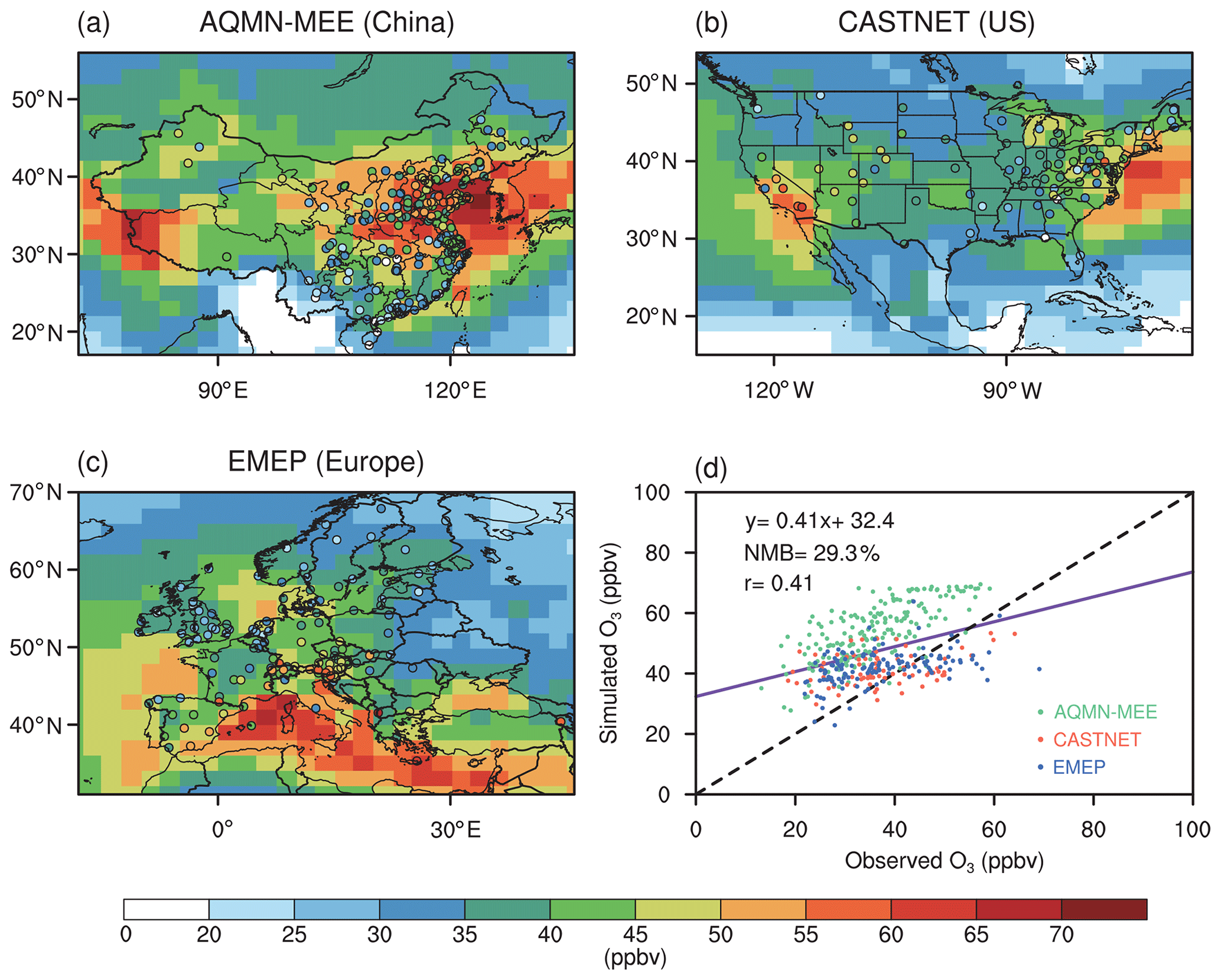
Figure 1Evaluations of simulated summer (June–August) daily (24 h average) surface O3 concentrations in the CTRL run. (a–c) Spatial distribution of observed O3 concentrations (circles) in AQMN-MEE in China, CASTNET in the US, and EMEP in Europe, respectively, and the simulated O3 concentrations. (d) Scatter plot of O3 concentrations (ppbv) over observational sites in the three regions. The x and y axes indicate the observed and simulated O3 concentrations, respectively. The purple line shows the linear regression between the observed and simulated O3 concentrations. The black dashed line shows the 1 : 1 lines.
To further compare the performance of ModelE2-YIBs with other chemistry–climate models, we select six simulated cases performed by different model members in the Atmospheric Chemistry and Climate Model Intercomparison Project (ACCMIP; Lamarque et al., 2013) and implement the evaluation with the same observational data (Fig. S2 in the Supplement). The correlation coefficient (0.41) and NMB (29.3 %) for ModelE2-YIBs are located in the ranges of 0.36 % to 0.60 % and −16.0 % to 45.1 % by the model ensembles, suggesting that ModelE2-YIBs has comparable performance to other state-of-the-art models. However, most of the current chemistry–climate models lack the interactive vegetation growth module, let alone studying O3–vegetation interactions. The vegetation variables (e.g. GPP and LAI) in ModelE2-YIBs have been fully evaluated in previous studies (Yue and Unger, 2015), making ModelE2-YIBs a suitable tool for this work.
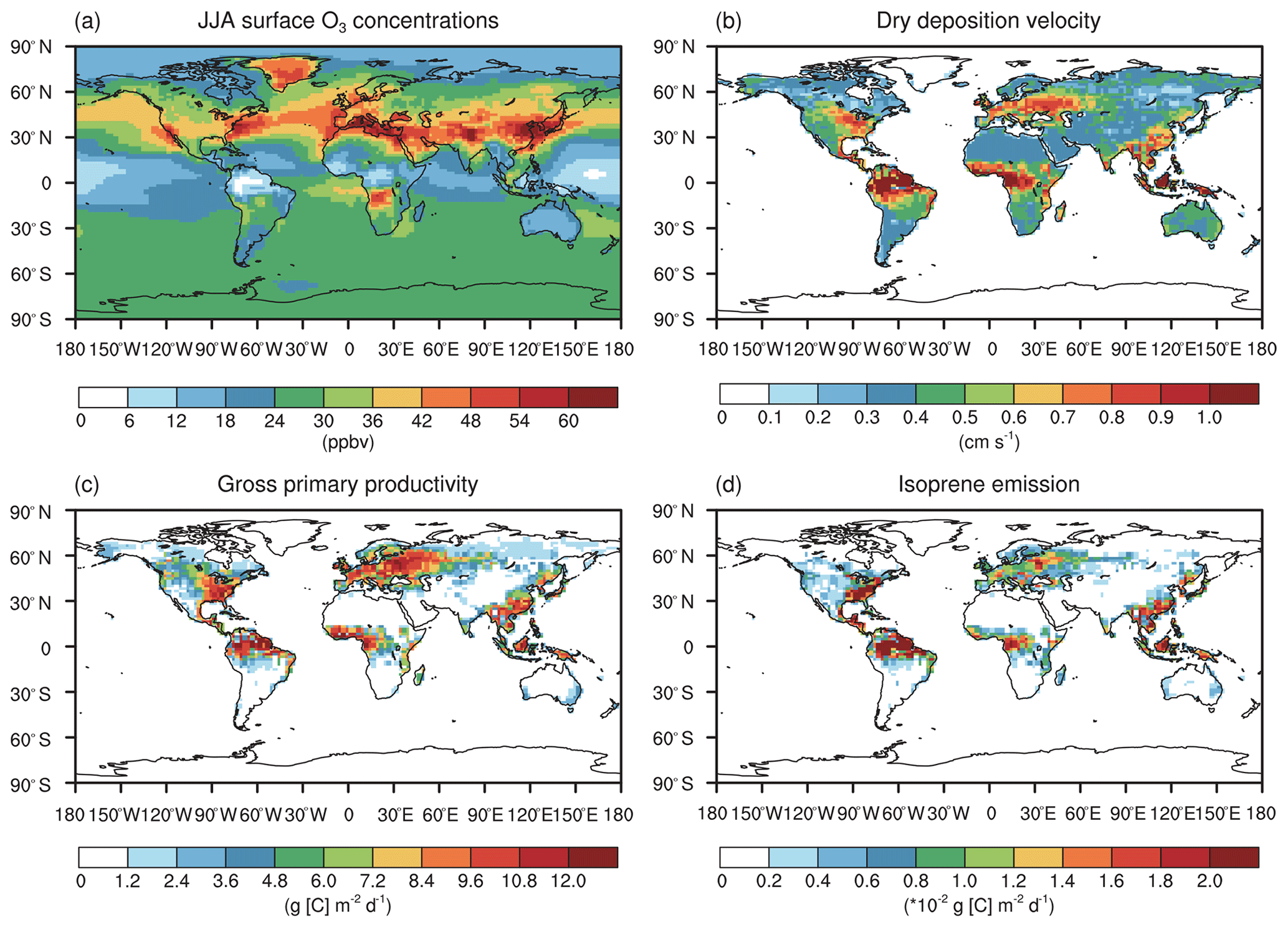
Figure 2The summer daily (a) surface O3 concentrations, (b) O3 dry deposition velocity, (c) gross primary productivity, and (d) isoprene emissions in the CTRL simulation without O3 damage to vegetation.
Figure 2 shows the global June–July–August (JJA) surface O3 concentrations, O3 dry deposition velocity, GPP, and IPE. Simulated O3 is high in the eastern US, western Europe, India, and eastern China (Fig. 2a). The spatial pattern of O3 dry deposition velocity (Fig. 2b) resembles that of the GPP (Fig. 2c) because the O3 stomatal uptake dominantly contributed to the dry deposition. Both are high in the eastern US, western Europe, Amazon, eastern China, and Indonesia and show a reasonable magnitude consistent with previous modeling studies (Val Martin et al., 2014; Yue and Unger, 2015; Sadiq et al., 2017). The spatial pattern of IPE (Fig. 2d) also resembles that of the GPP (Fig. 2c) except that the IPE in Europe are lower than those in other regions. Such discrepancies are likely attributed to the lower fraction of deciduous broadleaf forest, which provides a high yield of IPE (Potter et al., 2001).
3.2 Offline O3 damage to IPE
Figure 3 shows the effect of O3 damage to IPE during the boreal summer. For different schemes, reductions in IPE show a similar spatial distribution with significant damages in the eastern US, western Europe, and eastern China, where both O3 concentrations and vegetative cover are high. For the F scheme with high sensitivity, the damage mediated by the IPE can reach as high as 30 % in eastern China and >20 % in the eastern US and western Europe (Fig. 3a). However, the F scheme with low sensitivity predicts low damage of ∼10 % in these regions (Fig. 3b). At a global scale, IPE decrease by 1.2 %–3.2 % because of the O3 effect. The damage using the linear scheme is generally within the low-to-high range of predictions by using the F schemes. For the linear scheme, IPE in eastern China show the greatest damage of ∼15 %.
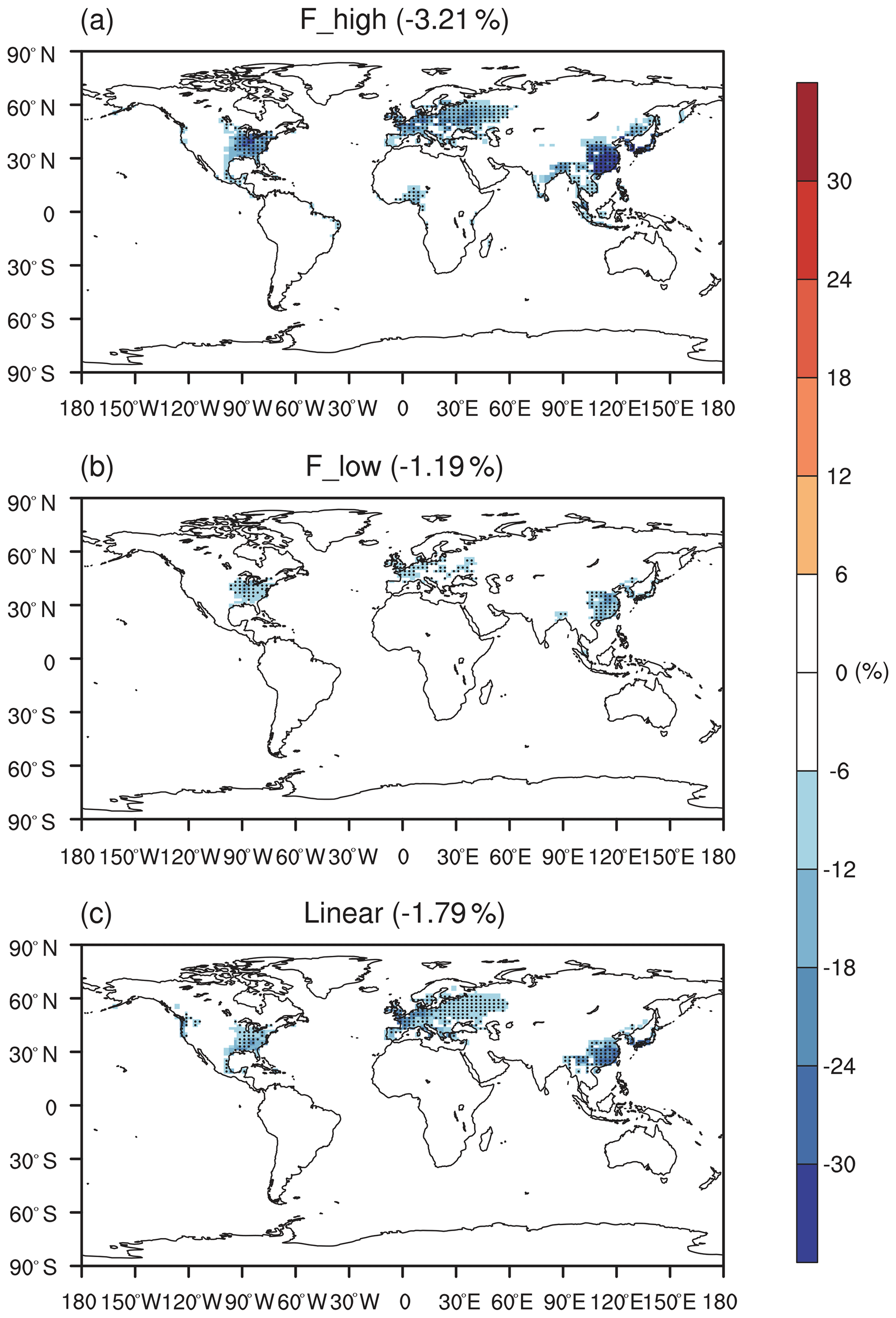
Figure 3Offline O3 damage (%) to IPE averaged over summer using the F scheme with (a) high or (b) low sensitivities and results obtained by using (c) the linear scheme. The dotted grids show significant damage at the 95 % confidence level. Global land area-weighted percentage changes in IPE are shown in the titles.
Figure 4 shows seasonal variations in the effect of O3 damage to IPE in eastern China, the eastern US, and western Europe. The magnitude of IPE changes is generally within the range of 10 %–29 %, as summarized by the observational meta-analysis (Feng et al., 2019b). The F scheme is dependent on instantaneous O3 uptake, which peaks during the summer when both surface O3 and stomatal conductance are high. In contrast, the linear scheme depends on the accumulated O3 flux, which increases from zero to high levels during the growth season. As shown, the percentage of O3 damage to IPE is low during April and May but increases to a similar magnitude to that in the F scheme with high sensitivity during August; it reaches a maximum in October. The differences in the F (instantaneous) and linear (accumulated) schemes cause distinct seasonal variations in the IPE damage, which might cause different feedback to the O3 concentrations. However, the IPE peaks during summer (Fig. S3 in the Supplement), suggesting that absolute changes in IPE are most significant during this season (Fig. S4 in the Supplement). Meanwhile, since the surface O3 concentrations and the vegetation growth both peak during boreal summer in the Northern Hemisphere, the O3–vegetation interactions are supposed to be the strongest in this season. As a result, we focus our analyses on the summer to explore the O3–vegetation interactions and feedback.
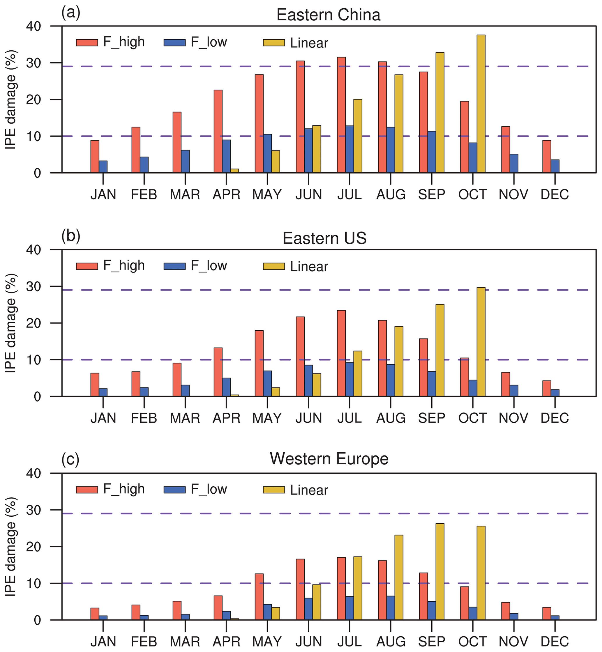
Figure 4Monthly mean percentage O3 damage to IPE averaged over (a) eastern China, (b) the eastern US, and (c) western Europe by using the F scheme with high and low sensitivities and the linear scheme, respectively. The dashed lines indicate the range of IPE damage summarized by observational meta-analysis.
3.3 O3–vegetation feedbacks on surface O3 concentrations
The effect of O3 damage to stomatal conductance inhibits dry deposition (Fig. S5 in the Supplement), leading to significant increases in summer surface O3, particularly in eastern China, Japan, the eastern US, and western Europe (Fig. 5a and b). The positive feedback can be greater than 5 ppbv in eastern China with high sensitivity (Fig. 5a). Smaller changes are predicted for low sensitivity, which shows limited perturbations in the US and Japan (Fig. 5b). Including the effect of O3 damage to both stomatal conductance and IPE maintains the spatial pattern of O3 changes but occurs at a lower magnitude (Fig. 5c–f) because these two effects offset each other. With high damage to stomatal conductance, surface O3 remains increasing in eastern China, Japan, the eastern US, and western Europe even with reduced IPE (Fig. 5c and e). However, with low damage to stomatal conductance, surface O3 shows limited changes in Europe, China, and Japan when IPE are simultaneously reduced (Fig. 5d and f). Surprisingly, surface O3 increases over the eastern US in these cases (Fig. 5d and f) compared to the limited changes when IPE remain unperturbed (Fig. 5b).
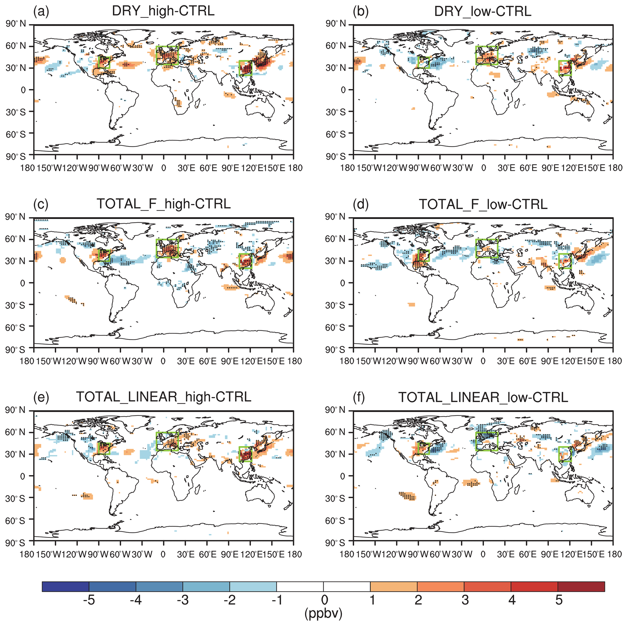
Figure 5O3–vegetation feedback on surface O3 concentrations during summer. The results shown are changes in surface O3 resulting from O3 damage to stomatal conductance alone with (a) high and (b) low sensitivity. In addition to stomatal conductance, O3 damage to IPE is also included by using the F scheme with (c) high and (d) low sensitivity. In comparison, O3 damage to IPE is added for the linear scheme in (e) and (f). The dotted grids indicate significant changes at the 95 % confidence level. The three regions in boxes denote eastern China, the eastern US, and western Europe.
Table 2Summary of the O3–vegetation feedbacks on summertime (June–August) mean surface O3 concentrations ([O3]), surface air temperature (T), surface relative humidity (RH), and isoprene emissions (IPE) in different sensitivity experiments. The values are calculated as the online differences between sensitivity and CTRL experiments. At each region, the minimum and maximum changes are shown as uncertainties.
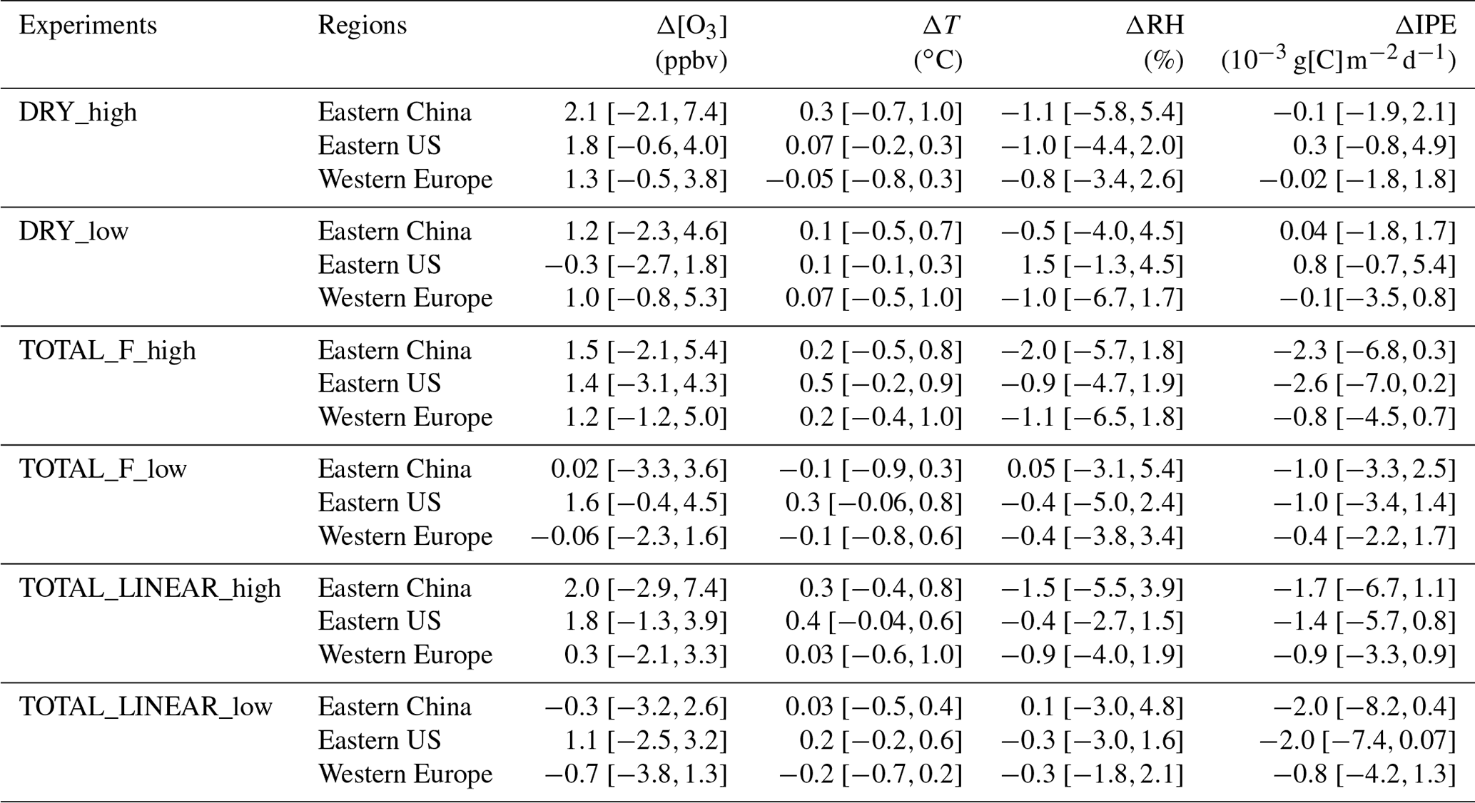
Figure 6 summarizes the changes in surface O3 over sensitive regions. Without IPE feedback, the effect of O3 damage to stomatal conductance leads to changes in regionally averaged surface O3 by +2.1 ppbv (+1.2 ppbv) in eastern China, +1.8 ppbv (−0.3 ppbv) in the eastern US, and +1.3 ppbv (+1.0 ppbv) in western Europe for high (low) damage sensitivity (Table 2). Changes in eastern China are the greatest compared to those of the other two regions, mainly because of the high O3 level (Fig. 1a) and sensitive tree species (the high a and low for deciduous broadleaf forest; Table S1). Surface O3 is predicted to decrease in the eastern US with the low damage sensitivity, though such a change is not significant over most grids (Fig. 5b). The inclusion of the effect of O3 damage for both stomatal conductance and IPE slightly weakens the O3 feedback, leading to changes in O3 concentrations of +1.5 ppbv (+0.02 ppbv) with the F scheme and +2.0 ppbv (−0.3 ppbv) with the linear scheme in eastern China for high (low) sensitivity. The regional maximum O3 changes can reach 7.4 ppbv (4.6 ppbv) in eastern China. Further, the effect of O3 damage to IPE weakens the positive feedback in western Europe by approximately 1–2 ppbv. The average O3 changes in the eastern US due to high (low) O3 damage are +1.4 ppbv (+1.6 ppbv) with the F scheme and +1.8 ppbv (+1.1 ppbv) with the linear scheme when IPE feedback is included.
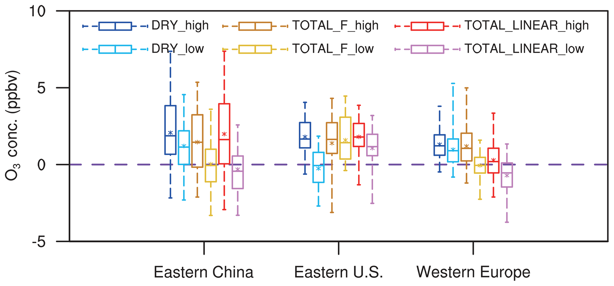
Figure 6Box plots of summer O3 changes in three sensitive regions among different sensitivity experiments. The error bars show the ranges of O3 changes in individual grids over the selected regions. Asterisks indicate the mean O3 changes averaged over the selected regions.
Although damage to stomatal conductance and IPE exert opposite effects, surface O3 in general increases after including both processes (Fig. 6), suggesting that dry deposition inhibition plays the dominant role. For the same high O3 damage sensitivity to stomatal conductance, changes in surface O3 remain similar over eastern China and the eastern US between the F and linear schemes in terms of the responses of the IPE (Table 2). However, responses in western Europe are weaker for the linear scheme (Fig. 5e) compared to that of the F scheme (Fig. 5c), though the former predicts lower reductions in IPE (Fig. 3). Nevertheless, inclusion of IPE reductions helps increase surface O3 over the eastern US (Fig. 5d and f vs. Fig. 5b), which is unexpected, since the reduction in IPE is supposed to decrease O3 concentrations. These changes are speculated to be indirectly related to O3–vegetation feedback to meteorology and would be further examined in the next section.
3.4 Effects of O3–vegetation interactions on meteorology and vegetation
Figures 7 and 8 show the changes in surface air temperature and relative humidity (RH) between different sensitivity experiments and the CTRL simulation, respectively. When considering the effect of O3 damage on stomatal conductance alone, eastern China becomes warmer (Fig. 7a and b) and drier (Fig. 8a and b), favoring O3 chemical production and increasing surface O3 concentrations (Jacob and Winner, 2009). The damaged stomatal conductance weakens leaf-level transpiration and thus reduces the latent heat flux at the surface (Fig. S6 in the Supplement), leading to a higher temperature and lower RH. The effect of O3 damage is weaker in the eastern US and western Europe because of the lower O3 concentrations, resulting in insignificant changes in temperature and RH over these regions.

Figure 7Same as Fig. 5 but for changes in surface air temperature.
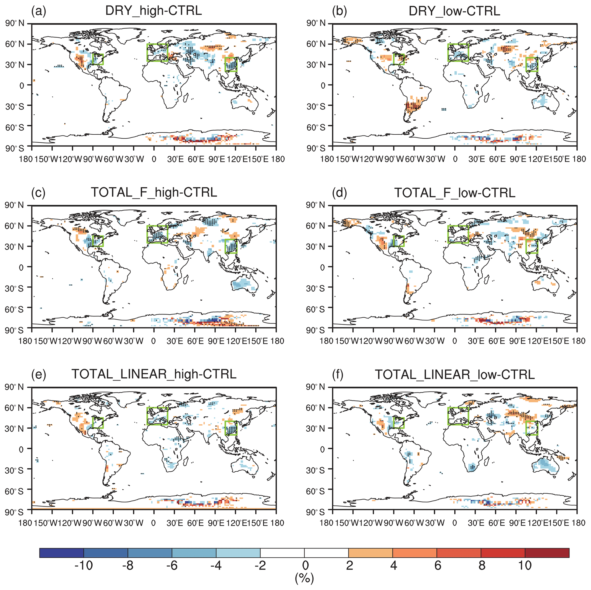
Figure 8Same as Fig. 5 but for changes in relative humidity.
The effect of O3 damage to IPE has limited impacts on RH (as shown in Fig. 8c and e vs. 8a and Fig. 8d and f vs. 8b) but significantly increases surface air temperature in the eastern US (as shown in Fig. 7c and e vs. 7a and Fig. 7d and f vs. 7b). The temperature in western Europe also slightly increases when IPE reductions are included, particularly when utilizing the F scheme with high sensitivity (Fig. 7c). Isoprene is among the most important precursors for the formation of SOAs (Claeys et al., 2004), which are able to reduce surface air temperature by light extinction (Charlson et al., 1992). As a result, the O3-induced reduction of IPE decreases SOA loading and weakens the “cooling effect” of aerosols, leading to a higher temperature at the surface. The positive changes in shortwave radiative forcing following SOA reduction are the strongest in the eastern US when considering the effect of O3 damage to IPE, particularly for the F schemes with high sensitivity (Fig. 9). Such warming explains why the reduced IPE help increase the surface O3 in the eastern US (Fig. 6). However, aerosols in regions with high anthropogenic emissions (such as eastern China) are more dominated by inorganic components (Sun et al., 2006; Yang et al., 2011); thus, the changes in SOAs are less important. As a result, the feedback of O3-induced IPE reductions on temperature is not significant in eastern China compared to that of other regions.
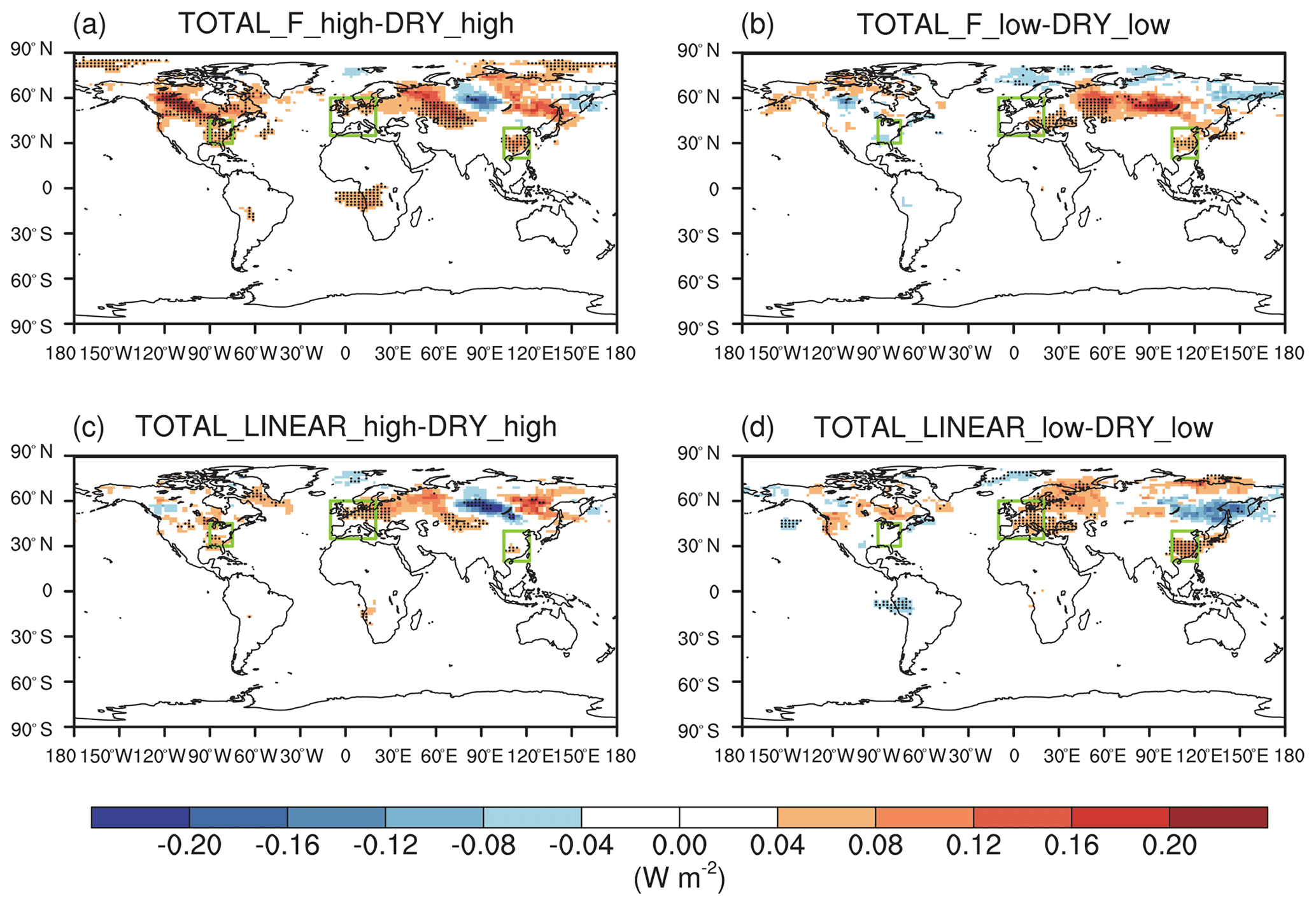
Figure 9Effects of O3-induced IPE reductions on SOA shortwave radiative forcing at the surface during the boreal summer. The impacts of O3 damage to IPE are isolated by determining the differences in the experiments for (a) high and (b) low sensitivities by using the F schemes or (c, d) the linear scheme. Dotted grids indicate significant changes at the 95 % confidence level.
In addition to the direct damage (Fig. 3), IPE are indirectly affected by perturbations in the LAI and meteorology. Figure S5 shows that the LAI decreases in three polluted regions (eastern China, the eastern US, and western Europe) because of the O3-mediated inhibition of photosynthesis, although the magnitude is typically within 5 %. Moderate changes in the LAI by O3 have also been reported in previous studies (Yue and Unger, 2015; Sadiq et al., 2017), suggesting that LAI feedback is too low to effectively influence IPE and the consequent surface O3. Furthermore, the warming effects resulting from the O3-induced inhibition on stomatal conductance (Fig. 7) and the changes in the LAI (Fig. S7 in the Supplement) cause limited changes in IPE (Fig. S8 in the Supplement), suggesting that O3–vegetation feedback does not significantly change IPE. In comparison, Sadiq et al. (2017) reported a strong positive feedback (3–5 times greater than our results) on IPE caused by increased temperature from reduced transpiration when the effect of O3 damage to stomatal conductance is considered. However, Sadiq et al. (2017) might have overestimated temperature feedback because their parameterizations of O3 damage to plants employ constant intercepts for some PFTs, which results in sustained damage even at low O3 concentrations.
In this study, we explore the effect of O3–vegetation feedback on surface O3 concentrations by considering the effects of O3 damage on photosynthesis, stomatal conductance, and IPE in a fully coupled global chemistry–carbon–climate model. Three regions with high O3 levels and dense vegetation cover, including eastern China, the eastern US, and western Europe, are examined during the summer. Results are summarized in Table 2. The positive feedback increases O3 concentrations on average by +2.1 ppbv (+1.2 ppbv) in eastern China, +1.8 ppbv (−0.3 ppbv) in the eastern US, and +1.3 ppbv (+1.0 ppbv) in western Europe for high (low) O3 damage to stomatal conductance and the consequent inhibition of dry deposition. Additionally, the effect of O3 damage to stomatal conductance increases the surface temperature and decreases the RH by weakening transpiration, which favors O3 chemical production and increases surface O3 concentrations. Including the effect of O3 damage to IPE slightly weakens the positive feedback in eastern China and western Europe but increases O3 concentrations especially with low O3 damaging sensitivity in the eastern US. The increased temperatures following reduced SOA concentrations are speculated to be a possible cause for this result. Our results show that O3–vegetation interactions increase surface O3 by reducing dry deposition (from inhibition of stomatal conductance) and increasing chemical formation (from surface warming by weakening transpiration and SOA radiative forcing). However, changes in precursor IPE as well as the LAI have limited impacts on surface O3.
Sadiq et al. (2017) also showed positive O3–vegetation feedback on the surface O3 in a global model. Compared to their results, we find an ultimate positive feedback with a similar magnitude of surface O3 concentrations but different spatial pattern. The strongest feedback is in eastern China rather than western Europe, which is more reasonable, as the O3 level in China is much higher than that in Europe (Lu et al., 2018). In addition, the effect of O3–vegetation feedback on temperature is lower in our study. The fixed decoupled scheme in Sadiq et al. (2017) may have overestimated the effect of O3 damage to stomatal conductance, leading to stronger feedback on O3 concentrations and temperature. Furthermore, the mechanisms of O3 effects on IPE are different. Sadiq et al. (2017) showed increased IPE because of the warming feedback. However, such warming is not significant in our study (Fig. S8 in the Supplement). Instead, we include the direct effect of O3 damage to IPE based on observations. Although the simulations show limited impacts of reduced IPE on surface O3, the simultaneously reduced SOAs contribute to increased surface O3 by weakening shortwave radiative forcing and increasing temperature in the eastern US.
Our results are subject to uncertainties in modeled O3 and damaging schemes. ModelE2-YIBs overestimates summer O3, particularly in China (Fig. 1), which may exacerbate the damage to stomatal conductance and the consequent feedback. The O3 damage parameterization by Sitch et al. (2007) is a semiphysical scheme that couples photosynthesis and stomatal conductance. However, some observational studies have showed that the sluggish stomatal responses under chronic O3 exposure lead to stomata losing function and decoupling from photosynthesis (Paoletti and Grulke, 2005; Gregg et al., 2006). The decoupled parameterization proposed by Lombardozzi et al. (2012) has been applied to estimate the effect of O3 damage to photosynthesis and stomatal conductance (Lombardozzi et al., 2015; Sadiq et al., 2017; Zhou et al., 2018). Nevertheless, we apply the parameterization by Sitch et al. (2007) because the damage is reasonably associated with the ambient O3 level, and the scheme has been extensively evaluated against available observations (Yue et al., 2017; Yue and Unger, 2018). Fixed damage for low (even zero) O3 included in some PFTs in the decoupled scheme may result in overestimation of O3–vegetation feedback in the global model.
To our knowledge, this is the first time that the effect of O3 damage to IPE is included in a fully coupled global chemistry–carbon–climate model. Both the F and linear schemes can simulate reasonable reductions in IPE compared to global meta-analysis, although with large uncertainties. The reduced IPE, as precursors, have insignificant effects on surface O3 concentrations in eastern China (Figs. 5 and 6), likely because of high anthropogenic emissions that undermine the feedback of IPE changes to surface O3. However, the reduced IPE weaken SOA radiative forcing and increase surface temperature in the eastern US, where biogenic SOAs provide important contributions to total aerosols (Fine et al., 2008; Goldstein et al., 2009). These results suggest that IPE feedback to the surface O3 is quite uncertain and dependent on ambient precursors (anthropogenic vs. biogenic) and oxidizing capacity (NOx-saturated vs. NOx-limited).
Variations in meteorological parameters may also influence O3–vegetation feedback. Plant stomata tend to close under drought stress to prevent water loss. As a result, dry climate may weaken O3–vegetation feedback through regulation of stomatal conductance (Lin et al., 2019). The effects of drought cannot be evaluated using ModelE2-YIBs, which simulates climatology with small interannual variability. In the future, a chemical transport model (CTM) coupled with a dynamic vegetation model (such as GC-YIBs developed by Lei et al., 2020) will be used to examine drought impacts by using observation-based meteorological forcings.
Despite these uncertainties, our analyses highlight the importance of O3–vegetation interactions in surface O3 concentrations. The feedback should be considered in regional and global air quality models for more realistic simulations. Furthermore, the effect of positive feedback on surface O3 may potentially aggravate O3 pollution in the future with increased ambient O3 under a warming climate (Lei et al., 2012; Doherty et al., 2013).
The observed hourly ozone concentrations for AQMN-MEE, CASTNET, and EMEP were obtained from the Data Center of China's Ministry of Ecology and Environment (http://datacenter.mee.gov.cn/websjzx/queryIndex.vm; DCDMEE, 2020), the US Environmental Protection Agency (https://java.epa.gov/castnet/clearsession.do; USEPA, 2020), and the EMEP Chemical Coordinating Centre (http://ebas.nilu.no/default.aspx; EMEPCCC, 2020). The source codes for the ModelE2-YIBs are available through collaboration. Please submit a request to Xu Yue (yuexu@nuist.edu.cn).
The supplement related to this article is available online at: https://doi.org/10.5194/acp-20-3841-2020-supplement.
XY conceived the study. CG carried out the simulations and performed the analysis. YL and YM provided useful comments on the paper. CG, XY, and HL prepared the paper, with contributions from all coauthors.
The authors declare that they have no conflict of interest.
We acknowledge the Data Center of China's Ministry of Ecology and Environment, the US Environmental Protection Agency, and the EMEP Chemical Coordinating Centre for making their data publicly available.
This research has been supported by the National Key Research and Development Program of China (grant no. 2019YFA0606802), the National Natural Science Foundation of China (grant nos. 41975155 and 91744311), and the Startup Foundation for Introducing Talent of NUIST.
This paper was edited by Frank Dentener and reviewed by two anonymous referees.
Ainsworth, E. A., Yendrek, C. R., Sitch, S., Collins, W. J., and Emberson, L. D.: The Effects of Tropospheric Ozone on Net Primary Productivity and Implications for Climate Change, Annu. Rev. Plant Biol., 63, 637–661, https://doi.org/10.1146/annurev-arplant-042110-103829, 2012.
Arneth, A., Niinemets, Ü., Pressley, S., Bäck, J., Hari, P., Karl, T., Noe, S., Prentice, I. C., Serça, D., Hickler, T., Wolf, A., and Smith, B.: Process-based estimates of terrestrial ecosystem isoprene emissions: incorporating the effects of a direct CO2-isoprene interaction, Atmos. Chem. Phys., 7, 31–53, https://doi.org/10.5194/acp-7-31-2007, 2007.
Atkinson, R.: Atmospheric chemistry of VOCs and NOx, Atmos. Environ., 34, 2063–2101, https://doi.org/10.1016/s1352-2310(99)00460-4, 2000.
Ball, J. T., Woodrow, I. E., and Berry, J. A.: A model predicting stomatal conductance and its contribution to the control of photosynthesis under different environmental conditions, Progr. Photosynth. Res., 4, 221–224, 1987.
Bian, H. S., Prather, M. J., and Takemura, T.: Tropospheric aerosol impacts on trace gas budgets through photolysis, J. Geophys. Res.-Atmos., 108, 4242, https://doi.org/10.1029/2002jd002743, 2003.
Broich, M., Huete, A., Paget, M., Ma, X., Tulbure, M., Coupe, N. R., Evans, B., Beringer, J., Devadas, R., Davies, K., and Held, A.: A spatially explicit land surface phenology data product for science, monitoring and natural resources management applications, Environ. Model. Softw., 64, 191–204, https://doi.org/10.1016/j.envsoft.2014.11.017, 2015.
Calfapietra, C., Mugnozza, G. S., Karnosky, D. F., Loreto, F., and Sharkey, T. D.: Isoprene emission rates under elevated CO2 and O3 in two field-grown aspen clones differing in their sensitivity to O3, New Phytol., 179, 55–61, https://doi.org/10.1111/j.1469-8137.2008.02493.x, 2008.
Calfapietra, C., Fares, S., and Lofeto, F.: Volatile organic compounds from Italian vegetation and their interaction with ozone, Environ. Pollut., 157, 1478–1486, https://doi.org/10.1016/j.envpol.2008.09.048, 2009.
Calfapietra, C., Fares, S., Manes, F., Morani, A., Sgrigna, G., and Loreto, F.: Role of Biogenic Volatile Organic Compounds (BVOC) emitted by urban trees on ozone concentration in cities: A review, Environ. Pollut., 183, 71–80, https://doi.org/10.1016/j.envpol.2013.03.012, 2013.
Charlson, R. J., Schwartz, S. E., Hales, J. M., Cess, R. D., Coakley, J. A., Hansen, J. E., and Hofmann, D. J.: Climate forcing by anthropogenic aerosols, Science, 255, 423–430, https://doi.org/10.1126/science.255.5043.423, 1992.
Chung, S. H. and Seinfeld, J. H.: Global distribution and climate forcing of carbonaceous aerosols, J. Geophys. Res.-Atmos., 107, 4407, https://doi.org/10.1029/2001jd001397, 2002.
Claeys, M., Graham, B., Vas, G., Wang, W., Vermeylen, R., Pashynska, V., Cafmeyer, J., Guyon, P., Andreae, M. O., Artaxo, P., and Maenhaut, W.: Formation of secondary organic aerosols through photooxidation of isoprene, Science, 303, 1173–1176, https://doi.org/10.1126/science.1092805, 2004.
Collatz, G. J., Ball, J. T., Grivet, C., and Berry, J. A.: Physiological and environmental-regulation of stomatal conductance, photosynthesis and transpiration – a model that includes a laminar boundary-layer, Agr. Forest Meteorol., 54, 107–136, https://doi.org/10.1016/0168-1923(91)90002-8, 1991.
DCDMEE: The Air Quality Monitoring Network from the Ministry of Ecology and Environment, available at: http://datacenter.mee.gov.cn/websjzx/queryIndex.vm, last access: 28 March 2020.
Doherty, R. M., Wild, O., Shindell, D. T., Zeng, G., MacKenzie, I. A., Collins, W. J., Fiore, A. M., Stevenson, D. S., Dentener, F. J., Schultz, M. G., Hess, P., Derwent, R. G., and Keating, T. J.: Impacts of climate change on surface ozone and intercontinental ozone pollution: A multi-model study, J. Geophys. Res.-Atmos., 118, 3744–3763, https://doi.org/10.1002/jgrd.50266, 2013.
EMEPCCC: The air quality monitoring network from European Monitoring and Evaluation Programme, available at: http://ebas.nilu.no/default.aspx, last access: 28 March 2020.
Fares, S., Oksanen, E., Lannenpaa, M., Julkunen-Tiitto, R., and Loreto, F.: Volatile emissions and phenolic compound concentrations along a vertical profile of Populus nigra leaves exposed to realistic ozone concentrations, Photosynth. Res., 104, 61–74, https://doi.org/10.1007/s11120-010-9549-5, 2010.
Farquhar, G. D., Caemmerer, S. V., and Berry, J. A.: A biochemical-model of photosynthetic CO2 assimilation in leaves of C-3 species, Planta, 149, 78–90, https://doi.org/10.1007/bf00386231, 1980.
Feng, Z., Shang, B., Gao, F., and Calatayud, V.: Current ambient and elevated ozone effects on poplar: A global meta-analysis and response relationships, Sci. Total Environ., 654, 832–840, https://doi.org/10.1016/j.scitotenv.2018.11.179, 2019a.
Feng, Z., Yuan, X., Fares, S., Loreto, F., Li, P., Hoshika, Y., and Paoletti, E.: Isoprene is more affected by climate drivers than monoterpenes: A meta-analytic review on plant isoprenoid emissions, Plant Cell Environ., 42, 1939–1949, https://doi.org/10.1111/pce.13535, 2019b.
Fine, P. M., Sioutas, C., and Solomon, P. A.: Secondary particulate matter in the United States: Insights from the particulate matter supersites program and related studies, J. Air Waste Manage. Assoc., 58, 234–253, https://doi.org/10.3155/1047-3289.58.2.234, 2008.
Fu, Y. and Liao, H.: Simulation of the interannual variations of biogenic emissions of volatile organic compounds in China: Impacts on tropospheric ozone and secondary organic aerosol, Atmos. Environ., 59, 170–185, https://doi.org/10.1016/j.atmosenv.2012.05.053, 2012.
Fuhrer, J., Skarby, L., and Ashmore, M. R.: Critical levels for ozone effects on vegetation in Europe, Environ. Pollut., 97, 91–106, https://doi.org/10.1016/s0269-7491(97)00067-5, 1997.
Gauderman, W. J., Avol, E., Gilliland, F., Vora, H., Thomas, D., Berhane, K., McConnell, R., Kuenzli, N., Lurmann, F., Rappaport, E., Margolis, H., Bates, D., and Peters, J.: The effect of air pollution on lung development from 10 to 18 years of age, New England J. Med., 351, 1057–1067, https://doi.org/10.1056/NEJMoa040610, 2004.
Goldstein, A. H., Koven, C. D., Heald, C. L., and Fung, I. Y.: Biogenic carbon and anthropogenic pollutants combine to form a cooling haze over the southeastern United States, P. Natl. Acad. Sci. USA, 106, 8835–8840, https://doi.org/10.1073/pnas.0904128106, 2009.
Gregg, J. W., Jones, C. G., and Dawson, T. E.: Physiological and developmental effects of O-3 on cottonwood growth in urban and rural sites, Ecol. Appl., 16, 2368–2381, https://doi.org/10.1890/1051-0761(2006)016[2368:padeoo]2.0.co;2, 2006.
Guenther, A., Karl, T., Harley, P., Wiedinmyer, C., Palmer, P. I., and Geron, C.: Estimates of global terrestrial isoprene emissions using MEGAN (Model of Emissions of Gases and Aerosols from Nature), Atmos. Chem. Phys., 6, 3181–3210, https://doi.org/10.5194/acp-6-3181-2006, 2006.
Guenther, A. B., Jiang, X., Heald, C. L., Sakulyanontvittaya, T., Duhl, T., Emmons, L. K., and Wang, X.: The Model of Emissions of Gases and Aerosols from Nature version 2.1 (MEGAN2.1): an extended and updated framework for modeling biogenic emissions, Geosci. Model Dev., 5, 1471–1492, https://doi.org/10.5194/gmd-5-1471-2012, 2012.
Hartikainen, K., Nerg, A.-M., Kivimaenpaa, M., Kontunen-Soppela, S., Maenpaa, M., Oksanen, E., Rousi, M., and Holopainen, T.: Emissions of volatile organic compounds and leaf structural characteristics of European aspen (Populus tremula) grown under elevated ozone and temperature, Tree Physiol., 29, 1163–1173, https://doi.org/10.1093/treephys/tpp033, 2009.
Henze, D. K. and Seinfeld, J. H.: Global secondary organic aerosol from isoprene oxidation, Geophys. Res. Lett., 33, L09812, https://doi.org/10.1029/2006gl025976, 2006.
Jacob, D. J. and Winner, D. A.: Effect of climate change on air quality, Atmos. Environ., 43, 51–63, https://doi.org/10.1016/j.atmosenv.2008.09.051, 2009.
Koch, D., Schmidt, G. A., and Field, C. V.: Sulfur, sea salt, and radionuclide aerosols in GISS ModelE, J. Geophys. Res.-Atmos., 111, D06206, https://doi.org/10.1029/2004jd005550, 2006.
Lamarque, J.-F., Emmons, L. K., Hess, P. G., Kinnison, D. E., Tilmes, S., Vitt, F., Heald, C. L., Holland, E. A., Lauritzen, P. H., Neu, J., Orlando, J. J., Rasch, P. J., and Tyndall, G. K.: CAM-chem: description and evaluation of interactive atmospheric chemistry in the Community Earth System Model, Geosci. Model Dev., 5, 369–411, https://doi.org/10.5194/gmd-5-369-2012, 2012.
Lamarque, J.-F., Shindell, D. T., Josse, B., Young, P. J., Cionni, I., Eyring, V., Bergmann, D., Cameron-Smith, P., Collins, W. J., Doherty, R., Dalsoren, S., Faluvegi, G., Folberth, G., Ghan, S. J., Horowitz, L. W., Lee, Y. H., MacKenzie, I. A., Nagashima, T., Naik, V., Plummer, D., Righi, M., Rumbold, S. T., Schulz, M., Skeie, R. B., Stevenson, D. S., Strode, S., Sudo, K., Szopa, S., Voulgarakis, A., and Zeng, G.: The Atmospheric Chemistry and Climate Model Intercomparison Project (ACCMIP): overview and description of models, simulations and climate diagnostics, Geosci. Model Dev., 6, 179–206, https://doi.org/10.5194/gmd-6-179-2013, 2013.
Lane, T. E., Donahue, N. M., and Pandis, S. N.: Effect of NOx on secondary organic aerosol concentrations, Environ. Sci. Technol., 42, 6022–6027, https://doi.org/10.1021/es703225a, 2008.
Lei, H., Wuebbles, D. J., and Liang, X.-Z.: Projected risk of high ozone episodes in 2050, Atmos. Environ., 59, 567–577, https://doi.org/10.1016/j.atmosenv.2012.05.051, 2012.
Lei, Y., Yue, X., Liao, H., Gong, C., and Zhang, L.: Implementation of Yale Interactive terrestrial Biosphere model v1.0 into GEOS-Chem v12.0.0: a tool for biosphere–chemistry interactions, Geosci. Model Dev., 13, 1137–1153, https://doi.org/10.5194/gmd-13-1137-2020, 2020.
Lelieveld, J., Evans, J. S., Fnais, M., Giannadaki, D., and Pozzer, A.: The contribution of outdoor air pollution sources to premature mortality on a global scale, Nature, 525, 367–371, https://doi.org/10.1038/nature15371, 2015.
Li, K., Jacob, D. J., Liao, H., Shen, L., Zhang, Q., and Bates, K. H.: Anthropogenic drivers of 2013–2017 trends in summer surface ozone in China, P. Natl. Acad. Sci. USA, 116, 422–427, https://doi.org/10.1073/pnas.1812168116, 2019.
Lin, M., Malyshev, S., Shevliakova, E., Paulot, F., Horowitz, L. W., Fares, S., Mikkelsen, T. N., and Zhang, L.: Sensitivity of Ozone Dry Deposition to Ecosystem-Atmosphere Interactions: A Critical Appraisal of Observations and Simulations, Global Biogeochem. Cy., 33, 1264–1288, https://doi.org/10.1029/2018gb006157, 2019.
Liu, Z. Y., Notaro, M., Kutzbach, J., and Liu, N.: Assessing global vegetation-climate feedbacks from observations, J. Climate, 19, 787–814, https://doi.org/10.1175/jcli3658.1, 2006.
Lombardozzi, D., Levis, S., Bonan, G., and Sparks, J. P.: Predicting photosynthesis and transpiration responses to ozone: decoupling modeled photosynthesis and stomatal conductance, Biogeosciences, 9, 3113–3130, https://doi.org/10.5194/bg-9-3113-2012, 2012.
Lombardozzi, D., Levis, S., Bonan, G., Hess, P. G., and Sparks, J. P.: The Influence of Chronic Ozone Exposure on Global Carbon and Water Cycles, J. Climate, 28, 292–305, https://doi.org/10.1175/jcli-d-14-00223.1, 2015.
Lu, X., Hong, J. Y., Zhang, L., Cooper, O. R., Schultz, M. G., Xu, X. B., Wang, T., Gao, M., Zhao, Y. H., and Zhang, Y. H.: Severe Surface Ozone Pollution in China: A Global Perspective, Environ. Sci. Technol. Lett., 5, 487–494, https://doi.org/10.1021/acs.estlett.8b00366, 2018.
Menon, S., Unger, N., Koch, D., Francis, J., Garrett, T., Sednev, I., Shindell, D., and Streets, D.: Aerosol climate effects and air quality impacts from 1980 to 2030, Environ. Res. Lett., 3, 024004, https://doi.org/10.1088/1748-9326/3/2/024004, 2008.
Menon, S., Koch, D., Beig, G., Sahu, S., Fasullo, J., and Orlikowski, D.: Black carbon aerosols and the third polar ice cap, Atmos. Chem. Phys., 10, 4559–4571, https://doi.org/10.5194/acp-10-4559-2010, 2010.
Moore, C. E., Brown, T., Keenan, T. F., Duursma, R. A., van Dijk, A. I. J. M., Beringer, J., Culvenor, D., Evans, B., Huete, A., Hutley, L. B., Maier, S., Restrepo-Coupe, N., Sonnentag, O., Specht, A., Taylor, J. R., van Gorsel, E., and Liddell, M. J.: Reviews and syntheses: Australian vegetation phenology: new insights from satellite remote sensing and digital repeat photography, Biogeosciences, 13, 5085–5102, https://doi.org/10.5194/bg-13-5085-2016, 2016.
Paoletti, E. and Grulke, N. E.: Does living in elevated CO2 ameliorate tree response to ozone? A review on stomatal responses, Environ. Pollut., 137, 483–493, https://doi.org/10.1016/j.envpol.2005.01.035, 2005.
Potter, C. S., Alexander, S. E., Coughlan, J. C., and Klooster, S. A.: Modeling biogenic emissions of isoprene: exploration of model drivers, climate control algorithms, and use of global satellite observations, Atmos. Environ., 35, 6151–6165, https://doi.org/10.1016/s1352-2310(01)00390-9, 2001.
Presto, A. A., Hartz, K. E. H., and Donahue, N. M.: Secondary organic aerosol production from terpene ozonolysis. 2. Effect of NOx concentration, Environ. Sci. Technol., 39, 7046–7054, https://doi.org/10.1021/es050400s, 2005.
Ryan, A., Cojocariu, C., Possell, M., Davies, W. J., and Hewitt, C. N.: Defining hybrid poplar (Populus deltoides × Populus trichocarpa) tolerance to ozone: identifying key parameters, Plant Cell Environ., 32, 31–45, https://doi.org/10.1111/j.1365-3040.2008.01897.x, 2009.
Sadiq, M., Tai, A. P. K., Lombardozzi, D., and Val Martin, M.: Effects of ozone–vegetation coupling on surface ozone air quality via biogeochemical and meteorological feedbacks, Atmos. Chem. Phys., 17, 3055–3066, https://doi.org/10.5194/acp-17-3055-2017, 2017.
Schmidt, G. A., Kelley, M., Nazarenko, L., Ruedy, R., Russell, G. L., Aleinov, I., Bauer, M., Bauer, S. E., Bhat, M. K., Bleck, R., Canuto, V., Chen, Y.-H., Cheng, Y., Clune, T. L., Del Genio, A., de Fainchtein, R., Faluvegi, G., Hansen, J. E., Healy, R. J., Kiang, N. Y., Koch, D., Lacis, A. A., LeGrande, A. N., Lerner, J., Lo, K. K., Matthews, E. E., Menon, S., Miller, R. L., Oinas, V., Oloso, A. O., Perlwitz, J. P., Puma, M. J., Putman, W. M., Rind, D., Romanou, A., Sato, M., Shindell, D. T., Sun, S., Syed, R. A., Tausnev, N., Tsigaridis, K., Unger, N., Voulgarakis, A., Yao, M.-S., and Zhang, J.: Configuration and assessment of the GISS ModelE2 contributions to the CMIP5 archive, J. Adv. Model. Earth Syst., 6, 141–184, https://doi.org/10.1002/2013ms000265, 2014.
Sellers, P. J., Los, S. O., Tucker, C. J., Justice, C. O., Dazlich, D. A., Collatz, G. J., and Randall, D. A.: A revised land surface parameterization (SiB2) for atmospheric GCMs. 2. The generation of global fields of terrestrial biophysical parameters from satellite data, J. Climate, 9, 706–737, https://doi.org/10.1175/1520-0442(1996)009<0706:arlspf>2.0.co;2, 1996.
Sillman, S.: The relation between ozone, NOx and hydrocarbons in urban and polluted rural environments, Atmos. Environ., 33, 1821–1845, https://doi.org/10.1016/s1352-2310(98)00345-8, 1999.
Sitch, S., Cox, P. M., Collins, W. J., and Huntingford, C.: Indirect radiative forcing of climate change through ozone effects on the land-carbon sink, Nature, 448, 791–794, https://doi.org/10.1038/nature06059, 2007.
Spitters, C. J. T., Toussaint, H., and Goudriaan, J.: Separating the diffuse and direct component of global radiation and its implications for modeling canopy photosynthesis. 1. Components of incoming radiation, Agr. Forest Meteorol., 38, 217–229, https://doi.org/10.1016/0168-1923(86)90060-2, 1986.
Sun, Y., Zhuang, G., Tang, A., Wang, Y., and An, Z.: Chemical characteristics of PM2.5 and PM10 in haze-fog episodes in Beijing, Environ. Sci. Technol., 40, 3148–3155, https://doi.org/10.1021/es051533g, 2006.
Tiiva, P., Rinnan, R., Holopainen, T., Morsky, S. K., and Holopainen, J. K.: Isoprene emissions from boreal peatland microcosms; effects of elevated ozone concentration in an open field experiment, Atmos. Environ., 41, 3819–3828, https://doi.org/10.1016/j.atmosenv.2007.01.005, 2007.
Tucker, C. J., Slayback, D. A., Pinzon, J. E., Los, S. O., Myneni, R. B., and Taylor, M. G.: Higher northern latitude normalized difference vegetation index and growing season trends from 1982 to 1999, Int. J. Biometeorol., 45, 184–190, https://doi.org/10.1007/s00484-001-0109-8, 2001.
Unger, N.: Isoprene emission variability through the twentieth century, J. Geophys. Res.-Atmos., 118, 13606–13613, https://doi.org/10.1002/2013jd020978, 2013.
Unger, N., Harper, K., Zheng, Y., Kiang, N. Y., Aleinov, I., Arneth, A., Schurgers, G., Amelynck, C., Goldstein, A., Guenther, A., Heinesch, B., Hewitt, C. N., Karl, T., Laffineur, Q., Langford, B., A. McKinney, K., Misztal, P., Potosnak, M., Rinne, J., Pressley, S., Schoon, N., and Serça, D.: Photosynthesis-dependent isoprene emission from leaf to planet in a global carbon-chemistry-climate model, Atmos. Chem. Phys., 13, 10243–10269, https://doi.org/10.5194/acp-13-10243-2013, 2013.
USEPA: Clean Air Status and Trends Network from the US Environmental Protection Agency, available at: https://java.epa.gov/castnet/clearsession.do, last access: 28 March 2020.
Val Martin, M., Heald, C. L., and Arnold, S. R.: Coupling dry deposition to vegetation phenology in the Community Earth SystemModel: Implications for the simulation of surface O3, Geophys. Res. Lett., 41, 2988–2996, https://doi.org/10.1002/2014gl059651, 2014.
van Vuuren, D. P., Edmonds, J., Kainuma, M., Riahi, K., Thomson, A., Hibbard, K., Hurtt, G. C., Kram, T., Krey, V., Lamarque, J.-F., Masui, T., Meinshausen, M., Nakicenovic, N., Smith, S. J., and Rose, S. K.: The representative concentration pathways: an overview, Climatic Change, 109, 5–31, https://doi.org/10.1007/s10584-011-0148-z, 2011.
Velikova, V., Tsonev, T., Pinelli, P., Alessio, G. A., and Loreto, F.: Localized ozone fumigation system for studying ozone effects on photosynthesis, respiration, electron transport rate and isoprene emission in field-grown Mediterranean oak species, Tree Physiol., 25, 1523–1532, https://doi.org/10.1093/treephys/25.12.1523, 2005.
Wang, G., Huang, Y., Wei, Y., Zhang, W., Li, T., and Zhang, Q.: Climate Warming Does Not Always Extend the Plant Growing Season in Inner Mongolian Grasslands: Evidence From a 30-Year In Situ Observations at Eight Experimental Sites, J. Geophys. Res.-Biogeo., 124, 2364–2378, https://doi.org/10.1029/2019jg005137, 2019.
Wang, T., Xue, L., Brimblecombe, P., Lam, Y. F., Li, L., and Zhang, L.: Ozone pollution in China: A review of concentrations, meteorological influences, chemical precursors, and effects, Sci. Total Environ., 575, 1582–1596, https://doi.org/10.1016/j.scitotenv.2016.10.081, 2017.
Wesely, M. L.: Parameterization of surface resistances to gaseous dry deposition in regional-scale numerical-models, Atmos. Environ., 23, 1293–1304, https://doi.org/10.1016/0004-6981(89)90153-4, 1989.
Wesely, M. L. and Hicks, B. B.: A review of the current status of knowledge on dry deposition, Atmos. Environ., 34, 2261–2282, https://doi.org/10.1016/s1352-2310(99)00467-7, 2000.
White, M. A., Nemani, R. R., Thornton, P. E., and Running, S. W.: Satellite evidence of phenological differences between urbanized and rural areas of the eastern United States deciduous broadleaf forest, Ecosystems, 5, 260–273, https://doi.org/10.1007/s10021-001-0070-8, 2002.
Wittig, V. E., Ainsworth, E. A., and Long, S. P.: To what extent do current and projected increases in surface ozone affect photosynthesis and stomatal conductance of trees? A meta-analytic review of the last 3 decades of experiments, Plant Cell Environ., 30, 1150–1162, https://doi.org/10.1111/j.1365-3040.2007.01717.x, 2007.
Wu, L., Zhang, J., and Dong, W.: Vegetation effects on mean daily maximum and minimum surface air temperatures over China, Chin. Sci. Bull., 56, 900–905, https://doi.org/10.1007/s11434-011-4349-7, 2011.
Xiao, X., Hagen, S., Zhang, Q., Keller, M., and Moore III, B.: Detecting leaf phenology of seasonally moist tropical forests in South America with multi-temporal MODIS images, Remote Sens. Environ., 103, 465–473, https://doi.org/10.1016/j.rse.2006.04.013, 2006.
Yang, F., Tan, J., Zhao, Q., Du, Z., He, K., Ma, Y., Duan, F., Chen, G., and Zhao, Q.: Characteristics of PM2.5 speciation in representative megacities and across China, Atmos. Chem. Phys., 11, 5207–5219, https://doi.org/10.5194/acp-11-5207-2011, 2011.
Yin, C., Pu, X., Xiao, Q., Zhao, C., and Liu, Q.: Effects of night warming on spruce root around non-growing season vary with branch order and month, Plant Soil, 380, 249–263, https://doi.org/10.1007/s11104-014-2090-0, 2014.
Yuan, X., Calatayud, V., Gao, F., Fares, S., Paoletti, E., Tian, Y., and Feng, Z.: Interaction of drought and ozone exposure on isoprene emission from extensively cultivated poplar, Plant Cell Environ., 39, 2276–2287, https://doi.org/10.1111/pce.12798, 2016.
Yuan, X., Feng, Z., Liu, S., Shang, B., Li, P., Xu, Y., and Paoletti, E.: Concentration-and flux-based dose-responses of isoprene emission from poplar leaves and plants exposed to an ozone concentration gradient, Plant Cell Environ., 40, 1960–1971, https://doi.org/10.1111/pce.13007, 2017.
Yue, X. and Unger, N.: Ozone vegetation damage effects on gross primary productivity in the United States, Atmos. Chem. Phys., 14, 9137–9153, https://doi.org/10.5194/acp-14-9137-2014, 2014.
Yue, X. and Unger, N.: The Yale Interactive terrestrial Biosphere model version 1.0: description, evaluation and implementation into NASA GISS ModelE2, Geosci. Model Dev., 8, 2399–2417, https://doi.org/10.5194/gmd-8-2399-2015, 2015.
Yue, X., Keenan, T. F., Munger, W., and Unger, N.: Limited effect of ozone reductions on the 20-year photosynthesis trend at Harvard forest, Glob. Change Biol., 22, 3750–3759, https://doi.org/10.1111/gcb.13300, 2016.
Yue, X., Unger, N., Harper, K., Xia, X., Liao, H., Zhu, T., Xiao, J., Feng, Z., and Li, J.: Ozone and haze pollution weakens net primary productivity in China, Atmos. Chem. Phys., 17, 6073–6089, https://doi.org/10.5194/acp-17-6073-2017, 2017.
Yue, X. and Unger, N.: Fire air pollution reduces global terrestrial productivity, Nat. Commun., 9, 5413, https://doi.org/10.1038/s41467-018-07921-4, 2018.
Zhou, S. S., Tai, A. P. K., Sun, S., Sadiq, M., Heald, C. L., and Geddes, J. A.: Coupling between surface ozone and leaf area index in a chemical transport model: strength of feedback and implications for ozone air quality and vegetation health, Atmos. Chem. Phys., 18, 14133–14148, https://doi.org/10.5194/acp-18-14133-2018, 2018.