the Creative Commons Attribution 4.0 License.
the Creative Commons Attribution 4.0 License.
 | 26 Mar 2020
Technical note: LIMS observations of lower stratospheric ozone in the southern polar springtime of 1978
V. Lynn Harvey
Arlin Krueger
Larry Gordley
John C. Gille
James M. Russell III
The Nimbus 7 Limb Infrared Monitor of the Stratosphere (LIMS) instrument operated from 25 October 1978 through 28 May 1979. This note focuses on its Version 6 (V6) data and indications of ozone loss in the lower stratosphere of the Southern Hemisphere subpolar region during the last week of October 1978. We provide profiles and maps that show V6 ozone values of only 2 to 3 ppmv at 46 hPa within the edge of the polar vortex near 60∘ S from late October through mid-November 1978. There are also low values of V6 nitric acid (∼3 to 6 ppbv) and nitrogen dioxide (< 1 ppbv) at the same locations, indicating that conditions were suitable for a chemical loss of Antarctic ozone some weeks earlier. These “first light” LIMS observations provide the earliest space-based view of conditions within the lower stratospheric ozone layer of the southern polar region in springtime.


The Nimbus 7 Total Ozone Mapping Spectrometer (TOMS) provided the first daily image of total ozone for the Southern Hemisphere (SH) on 1 November 1978. That image in Fig. 1 shows an equatorward extension of the region of low-polar total column ozone (TCO) between 90 and 135∘ E. Minimum TCO is of the order of 270 Dobson units (DU) at 75∘ S, 90∘ E on this day. As a comparison, Farman et al. (1985) reported ground-based measurements of total ozone of about 225 DU on 1 November for 1980–1984 at Halley Bay (76∘ S, 333∘ E) and of about 270 DU at the Argentine Islands (65∘ S, 296∘ E) (see also TOMS total ozone values of Table 2 in Stolarski et al., 1986). We note, however, that those values are higher than 220 DU, “definition of the threshold for ozone hole conditions” (WMO, 2018).
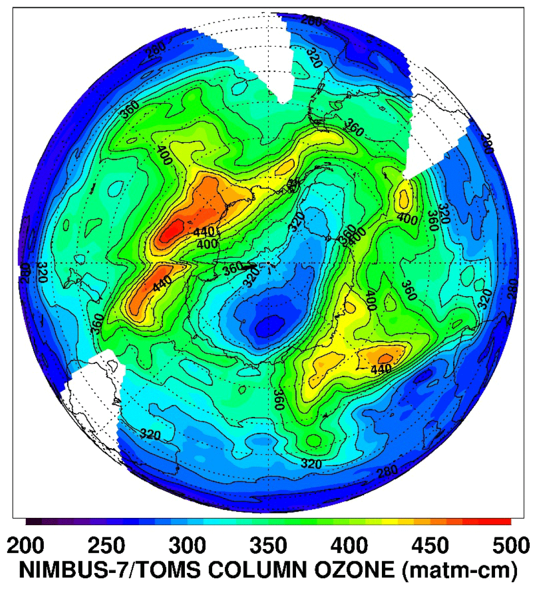
Figure 1Southern Hemisphere image of total column ozone (TCO) from TOMS for 1 November 1978. Longitude orientation is 0∘ E to the right and 90∘ E at the bottom; latitude circles (dotted) have a spacing of 10∘. White areas indicate where there are discrete data voids or no measurements. Ozone units of matm-cm are equivalent to Dobson units (DU), where 1 DU is 2.687×10²⁰ molecules per square meter. Black contours are TCO at intervals of 20 matm-cm.
There are very few observations of lower stratospheric ozone above Antarctica prior to November 1978, especially for the months of September and October when the seasonal loss of ozone is most significant (WMO, 2018). The historic Nimbus 7 Limb Infrared Monitor of the Stratosphere (LIMS) experiment (Gille and Russell III, 1984) provided data for middle atmosphere temperature, geopotential height (GPH), ozone, water vapor (H2O), nitric acid vapor (HNO3), and nitrogen dioxide (NO2) from 25 October 1978 through 28 May 1979, for scientific analysis and for comparisons with atmospheric models (e.g., Langematz et al., 2016). Remsberg et al. (2007) provide a description of its Version 6 (V6) ozone profiles. The mapping of the V6 profiles to the LIMS Level 3 product employs a sequential estimation algorithm with a relaxation time of about 2.5 d for analyses of its zonal six-wavenumber Fourier coefficients at each of 28 pressure levels of the middle atmosphere (Remsberg and Lingenfelser, 2010). We then generated daily polar stereographic plots of V6 ozone and HNO3 on pressure surfaces based on a gridding (2∘ latitude and 5.625∘ longitude) from those coefficients.
This note focuses on the character of the polar vortex and of the V6 ozone, HNO3, and NO2 in that region of the lower stratosphere during the last week of October 1978. The LIMS measurements extend to only 64∘ S, due to the orbital inclination of Nimbus 7 and to the viewing geometry of the LIMS instrument (Gille and Russell, 1984). We will show that the profiles and pressure surface maps indicate that there was a loss of SH polar ozone during the springtime. Section 2 contains plots that show a loss of ozone inside the vortex in late October. Section 3 reports on evidence for a denitrification of the air in the same region, indicating that there was a chemical loss of ozone some weeks earlier. Section 3 also presents time versus longitude or Hovmöller diagrams that reveal good correspondence for the low ozone and HNO3 values within the vortex region well into November. Section 4 summarizes the findings.
Figure 2 shows SH polar plots of V6 ozone mixing ratios at 46.4 hPa for 26 October and for 1 November, where the orbital measurements of LIMS extend only to 64∘ S. The plot on the right shows that there are minimum ozone values of about 2.6 ppmv near 120 and 315∘ E at 60∘ S on 1 November, which agrees reasonably with the locations of low total ozone from the TOMS image of Fig. 1. Ozone is of the order of 3.5 to 4 ppmv at most other longitudes. Low ozone occurs within the edges of the polar vortex, based on the concurrent GPH field from the operational ECMWF Reanalysis or ERA-40 products (Uppala et al., 2005). The bold contour in Fig. 2 denotes the edge of the vortex, in the manner of Harvey et al. (2002). We define the vortex edge as the streamfunction contour coincident with maximum wind speed that also encloses a region of rotation. Meek et al. (2017) showed that this definition of the vortex edge is in good agreement with the definition of Nash et al. (1996) based on the potential vorticity gradient. We note that daily plots of GPH are also available from LIMS V6. However, they exhibit a discontinuous anomaly at the 46 hPa level for the vortex region between 29 and 31 October, due to an interpolation of National Meteorological Center (NMC) GPH analyses supplied to the Nimbus-7 Project and used for the baseline pressure level of 50 hPa for the V6 GPH product (Remsberg et al., 2004). V6 geometric height and GPH profiles above and below that level are the result of a hydrostatic integration of the LIMS-retrieved temperature versus pressure profiles of Tp. Maps of V6 GPS farther away from the 50 hPa level are very similar to those from ERA-40.

Figure 2V6 ozone mixing ratios at 46.4 hPa for 26 October and 1 November 1978. Polar plots extend from 30∘ S to the South Pole and longitude is in ∘ E with 0∘ at right. Bold contours denote the vortex edge from ERA-40. The superposed, three colored dots correspond to the locations of profiles on 26 October (black and red) and on 3 September (green) in Fig. 3.
LIMS began its daily observations one week earlier than TOMS or on 25 October, and the left plot of Fig. 2 shows that the ozone for 26 October at 31∘ E is about half of that at 119∘ E on 1 November. The vortex on 26 October extends toward lower latitudes from about 60∘ S, 40∘ E. Both the vortex and region of low ozone deform and undergo a clockwise rotation from 26 October onward, such that their low values extend equatorward at 120 and at 315∘ E on 1 November. Bodeker et al. (2002) reported that the edge of the vortex often extends to near 60∘ S during October, and Stolarski et al. (1986, their Fig. 1) and Hassler et al. (2011) reported on an analogous clockwise rotation of the vortex during October.
The location of the vortex edge is helpful in deciding which V6 species profiles one ought to examine with regard to any constraints from HNO3 and NO2 on the ozone chemistry. As an example, Fig. 3 shows V6 Level 2 ozone profile segments from 11.4 to 88 hPa for two locations on 26 October, where ozone is now presented in units of partial pressure (in mPa) for a better delineation of its relative changes in the subpolar lower stratosphere. Estimates of accuracy for single V6 ozone profiles are 14 %, 26 %, and 34 % for 10, 50, and 100 hPa, respectively (see row (g) of Table 1 in Remsberg et al., 2007). The V6 ozone profile (black solid) at 54.9∘ S, 119∘ E is just outside the October 26 vortex, as shown by the black dot in Fig. 2, and its ozone values are nominal for subpolar latitudes. The largest contribution to total ozone from that profile in Fig. 3 occurs at the 68 hPa level. A second V6 ozone profile (solid red) is from 59.5∘ S, 31∘ E, and it is in a region of lower GPH as shown by the red dot in Fig. 2. Its ozone decreases rapidly from ∼8.0 mPa at the 53 hPa level to 2.6 mPa at the 88 hPa level, indicating a significant loss of ozone in the lower stratosphere sometime prior to 26 October. Komhyr et al. (1988, their Fig. 10) and Gernandt (1987) show from ozonesonde measurements that most of the observed losses of ozone for the mid-1980s occurred in the vortex in September and early October. Therefore, we also include in Fig. 3 an ozonesonde profile (solid green) from Syowa station (69∘ S, 40∘ E – the green dot in Fig. 2) for 3 September 1978, perhaps before there were any pronounced losses of ozone. Its ozone profile values are intermediate of those for the two V6 profiles of 26 October.

Figure 3V6 Level 2 species profiles for 59.5∘ S, 31∘ E (red) and 54.9∘ S, 119.4∘ E (black) on 26 October 1978, and from an ozonesonde at Syowa (69∘ S, 40∘ E – green) on 3 September 1978. Ozone (solid) has units of millipascals (mPa), while HNO3 (dashed) and NO2 (dot-dashed) have units of ppbv.
Loss of ozone due to reactive chlorine chemistry proceeds effectively in the presence of air that has undergone denitrification (Solomon, 1999; Müller et al., 2008). Lambert et al. (2016) somewhat loosely set an HNO3 threshold of < 5 ppbv for indicating denitrification at 46 hPa, based on Microwave Limb Sounder (MLS) data of 2008. Nitrous oxide is the source molecule for odd nitrogen (mainly HNO3) in the lower stratosphere, and its tropospheric values have grown by only a small amount from 1975 (∼296 ppbv) through 2008 (∼322 ppbv) (WMO, 2018); the HNO3 threshold of 5 ppbv should also be representative of 1978. Thus, in Fig. 3 we also show the accompanying V6 profiles of HNO3 and nighttime NO2 for the same two locations on 26 October. HNO3 and NO2 at 31∘ E are a half (or 3 ppbv) and a third (or < 1 ppbv), respectively, of those at 119∘ E below about the 31 hPa level. Thus, both species indicate that there was a denitrification of the air in the vortex region and a likely loss of ozone due to reactive chlorine chemistry in the presence of polar stratospheric clouds (PSCs) several weeks earlier (Solomon, 1999; WMO, 2018). Although the V6 temperature at 31∘ E on 26 October was 206 K (at 53 hPa), it is normal to find temperatures in the Antarctic vortex that are below the chlorine activation threshold value of 195 K and in the presence of PSCs during September and early October (WMO, 2018).
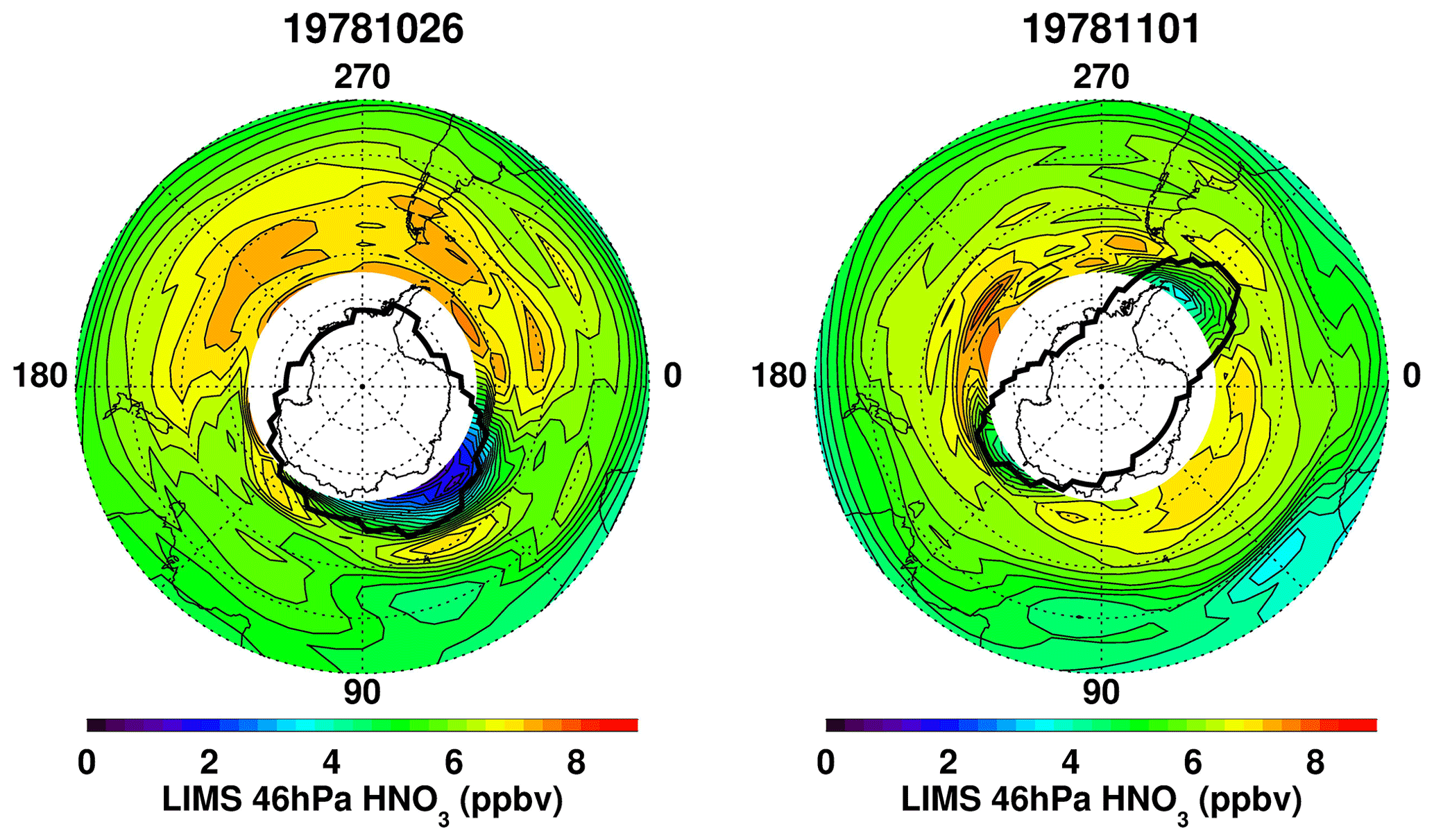
Figure 4As in Fig. 2, but for V6 HNO3.
Figure 4 shows the corresponding V6 plots of HNO3 at 46 hPa in terms of its mixing ratios, which have an estimated accuracy of ∼9 % (Remsberg et al., 2010, Table 10). There are very low values of HNO3 on 26 October poleward of 60∘ S and from 31∘ E to at least 90∘ E, indicating an earlier conversion of HNO3 from vapor to condensed phase and the sedimentation of larger HNO3 containing particles rather than an advection of low HNO3 from lower latitudes. Low HNO3 mixing ratios are also present within the vortex region on 1 November. Analogous polar plots of the nighttime NO2 fields are quite noisy (not shown) due to the large uncertainties for tangent layer NO2 in the lower stratosphere. Nevertheless, most of the odd nitrogen reservoir at 46 hPa comes from HNO3, not NO2. Together, they indicate the extent of denitrification of the air in the vortex region during late October 1978.
We show in Figs. 5 and 6 the details of the changing ozone and nitric acid from late October through November. Figure 5 displays time–longitude or Hovmöller diagrams for both species at 60∘ S; thick black contours indicate the vortex edge and dotted horizontal lines the vortex interior. The occurrence of lowest species mixing ratios is shown clearly in the vortex region in late October. Figure 6 extends the findings of Fig. 5 through the end of November, and there is an eastward progression of the region of low values from late October to early November. Reduced mixing ratios of those species occur inside the vortex until about 25 November, as expected for chemicals that are tracers of air motions in the lower stratosphere. The vortex distorts and then exhibits a stationary wave-1 pattern from November 5 onward, where height is lowest near 0∘ E. Mixing of air across the vortex edge appears slow for both ozone and HNO3 during that time.
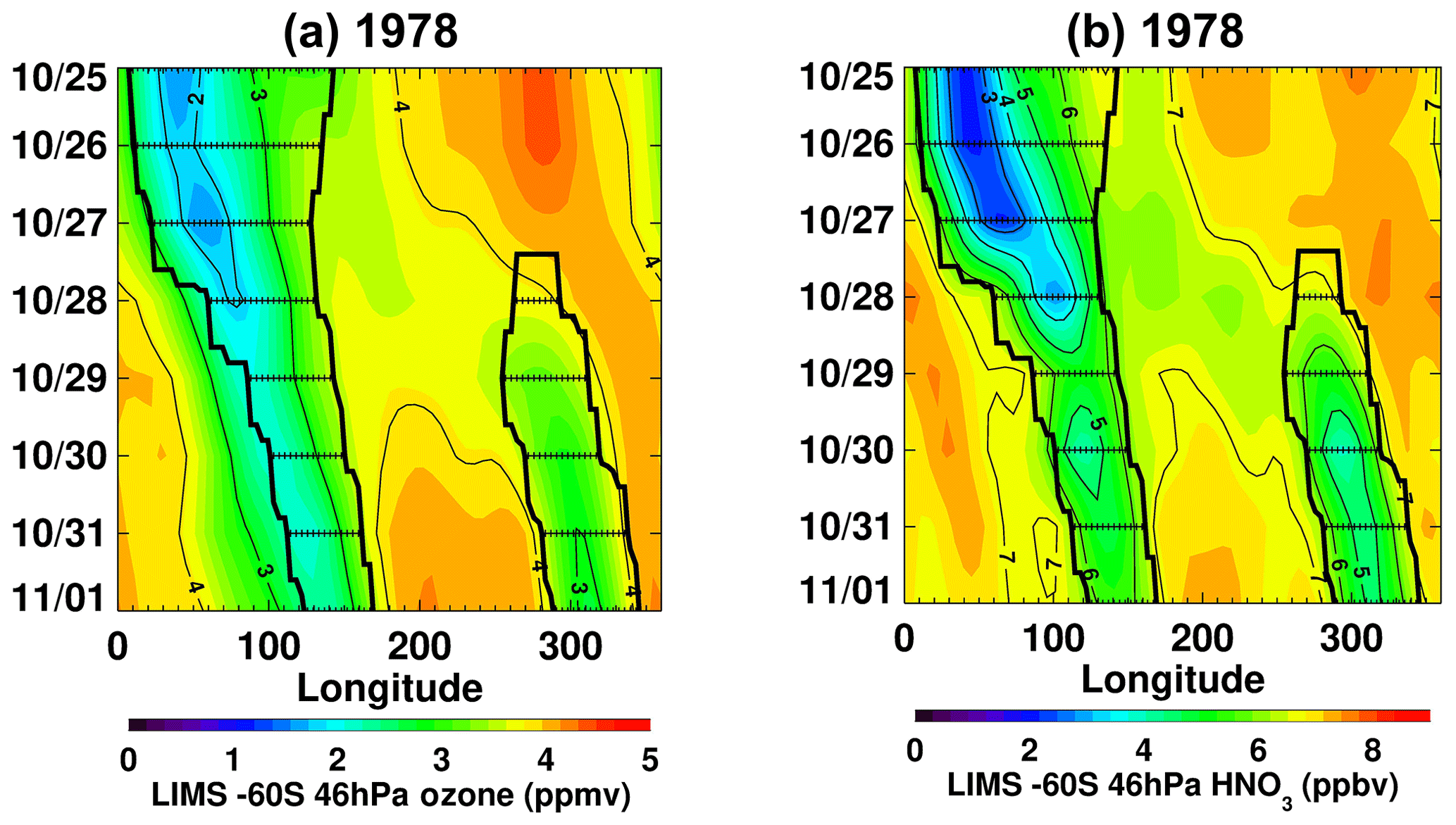
Figure 5Time–longitude or Hovmöller plots of LIMS ozone (a) and HNO3 (b) for 60∘ S and 46 hPa. The ERA-40 vortex edge is shown as thick black contours, and the vortex interior has horizontal dotted lines.
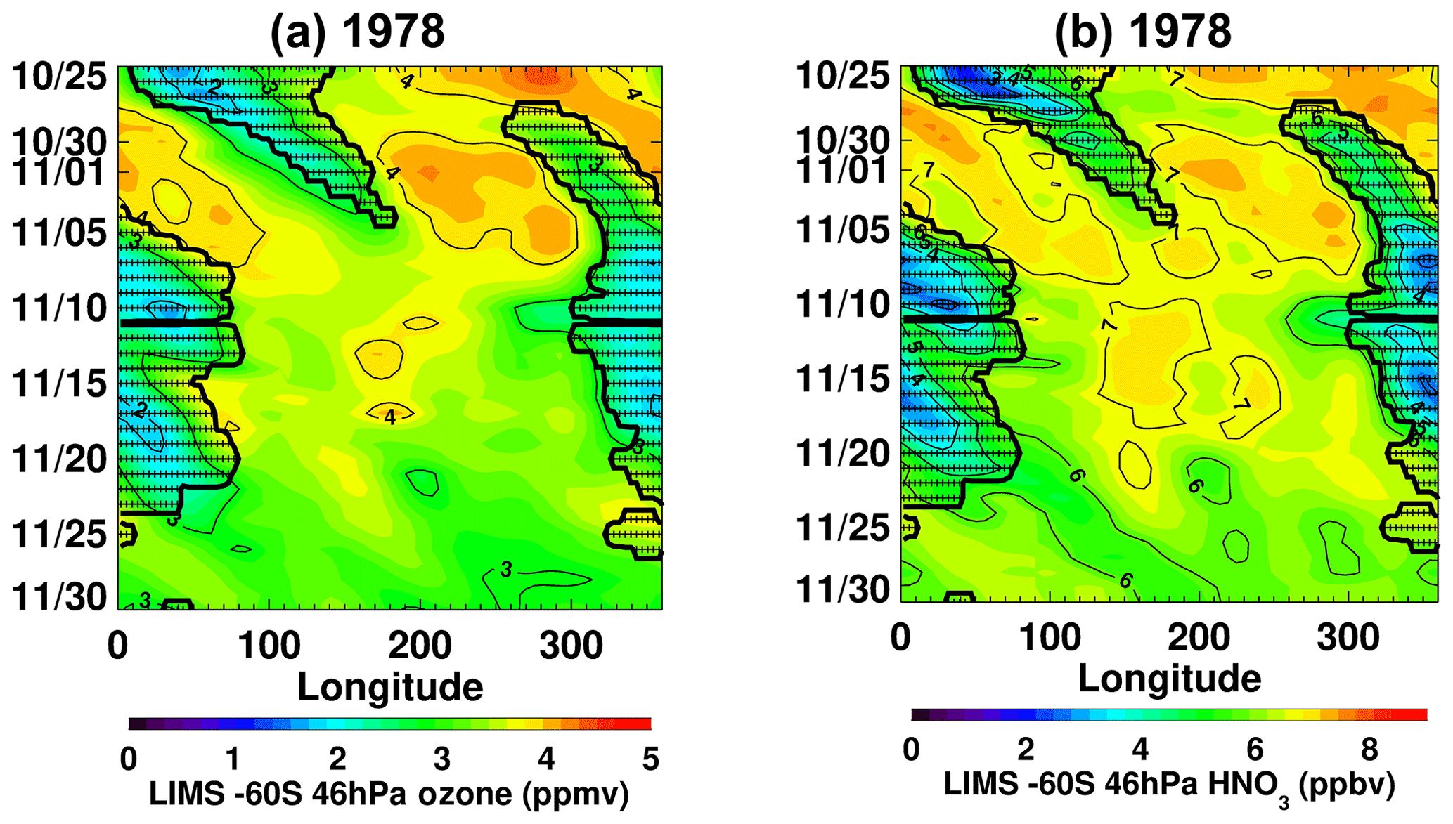
Figure 6As in Fig. 5, but extended in time from 25 October to 30 November 1978.
We find low V6 ozone mixing ratios of the order of 2 to 3 ppmv at 60∘ S within the edge of the polar vortex at 46 hPa during the last week of October and well into November 1978. There is good agreement between the V6 ozone map at 46 hPa and the TOMS image of total ozone in the region of the vortex on 1 November. Low V6 HNO3 mixing ratios of the order of 3 to 6 ppbv at the same locations indicate denitrification and conditions that were suitable for a chemical loss of Antarctic ozone some weeks earlier. We note that equivalent effective stratospheric chlorine (EESC) value of 2.01 ppbv used to predict conditions for the depletion of ozone in 1980 is about twice that of 1950, while the 1980 value is only half that of 2000 (Newman et al., 2007). In hindsight and based on the LIMS V6 dataset, we conclude that there was very likely some halogen-catalyzed loss of ozone in the southern polar vortex in winter and/or in spring of 1978. Yet, those ozone losses in the SH spring were not at the low level of a true “ozone hole” (< 220 DU total ozone). We also conclude that the LIMS V6 Level 2 profiles and the daily-analyzed maps from their Level 3 zonal coefficients represent useful comparison data for simulations of the expected changes in Antarctic ozone in spring 1978.
The LIMS V6 data archive is at the NASA EARTHDATA site of EOSDIS and its website: https://search.earthdata.nasa.gov/search?q=LIMS (Remsberg et al., 2020). Nimbus 7 TOMS ozone is at https://disc.gsfc.nasa.gov/datacollection/TOMSN7L2_008.html (TOMS Science Team, 2020). ECC ozonesonde ozone profiles are available from the World Ozone and Ultraviolet Radiation Data Centre or WOUDC at https://woudc.org/data/explore.php (WOUDC, 2020). ECMWF Reanalysis (ERA-40) data are accessible through https://climatedataguide.ucar.edu/climate-data/era40 (National Center for Atmospheric Research Staff, 2020).
ER and VLH wrote the manuscript and prepared the figures with input from all the other co-authors. AK provided information about the TOMS ozone images. LG led the development of the LIMS Version 6 algorithms. JCG and JMR are the co-principal investigators of the LIMS experiment. They also commented on the new insight from the findings about ozone and nitric acid of October 1978.
The authors declare that they have no conflict of interest.
VLH acknowledges support from NASA LWS grant NNX14AH54G, NASA HGI grant NNX17AB80G, and NASA HSR grant 80NSSC18K1046. Ellis Remsberg carried out his work while serving as a Distinguished Research Associate within the Science Directorate at NASA Langley.
This research has been supported by the NASA Langley Research Center (Science Directorate).
This paper was edited by Rolf Müller and reviewed by two anonymous referees.
Bodeker, G. E., Struthers, H., and Connor, B. J.: Dynamical containment of Antarctic ozone depletion, Geophys. Res. Lett., 29, 1098, https://doi.org/10.1029/2001GL014206, 2002.
Farman, J. C., Gardiner, B. G., and Shanklin, J. D.: Large losses of total ozone in Antarctica reveal seasonal ClOx∕NOx interaction, Nature, 315, 207–210, https://doi.org/10.1038/315207a0, 1985.
Gernandt, H.: The vertical ozone distribution above the GDR research base, Antarctica in 1985, Geophys. Res. Lett., 14, 84–66, 1987.
Gille, J. C. and Russell III, J. M.: The limb infrared monitor of the stratosphere: experiment description, performance, and results, J. Geophys. Res., 84, 5125–5140, https://doi.org/10.1029/JD089iD04p05125, 1984.
Harvey, V. L., Pierce, R. B., Fairlie, T. D., and Hitchman, M. H.: A climatology of stratospheric polar vortices and anticyclones, J. Geophys. Res., 107, 4442, https://doi.org/10.1029/2001JD001471, 2002.
Hassler, B., Bodeker, G. E., Solomon, S., and Young, P. J.: Changes in the polar vortex: effects on Antarctic total ozone observations at various stations, Geophys. Res. Lett., 38, L01805, https://doi.org/10.1029/2010GL045542, 2011.
National Center for Atmospheric Research Staff: The Climate Data Guide: ERA40, available at: https://climatedataguide.ucar.edu/climate-data/era40, last access: 23 March 2020.
WOUDC: Data Search/Download, available at: https://woudc.org/data/explore.php, last access: 23 March 2020.
Komhyr, W. D., Oltmans, S. J., and Grass, R. D.: Atmospheric ozone at South Pole, Antarctica, in 1986, J. Geophys. Res., 93, 5167–5184, https://doi.org/10.1029/JD093iD05p05167, 1988.
Lambert, A., Santee, M. L., and Livesey, N. J.: Interannual variations of early winter Antarctic polar stratospheric cloud formation and nitric acid observed by CALIOP and MLS, Atmos. Chem. Phys., 16, 15219–15246, https://doi.org/10.5194/acp-16-15219-2016, 2016.
Langematz, U., Schmidt, F., Kunze, M., Bodeker, G. E., and Braesicke, P.: Antarctic ozone depletion between 1960 and 1980 in observations and chemistry–climate model simulations, Atmos. Chem. Phys., 16, 15619–15627, https://doi.org/10.5194/acp-16-15619-2016, 2016.
Meek, C. E., Manson, A. H., and Drummond, J. R.: Comparison of Aura MLS stratospheric chemical gradients with north polar vortex edges calculated by two methods, Adv. Space Res., 60, 1898–1904, https://doi.org/10.1016/j.asr.2017.06.009, 2017.
Müller, R., Grooß, J.-U., Lemmen, C., Heinze, D., Dameris, M., and Bodeker, G.: Simple measures of ozone depletion in the polar stratosphere, Atmos. Chem. Phys., 8, 251–264, https://doi.org/10.5194/acp-8-251-2008, 2008.
Nash, E. R., Newman, P. A., Rosenfield, J. E., and Schoeberl, M. R.: An objective determination of the polar vortex using Ertel's potential vorticity, J. Geophys. Res., 101, 9471–9478, 1996.
Newman, P. A., Daniel, J. S., Waugh, D. W., and Nash, E. R.: A new formulation of equivalent effective stratospheric chlorine (EESC), Atmos. Chem. Phys., 7, 4537–4552, https://doi.org/10.5194/acp-7-4537-2007, 2007.
Remsberg, E. and Lingenfelser, G.: LIMS Version 6 Level 3 dataset, NASA-TM-2010-216690, available at: http://www.sti.nasa.gov (last access: 17 September 2019), 13 pp., 2010.
Remsberg, E., Lingenfelser, G., Natarajan, M., Gordley, L., Marshall, B. T., and Thompson, E.: On the quality of the Nimbus 7 LIMS version 6 ozone for studies of the middle atmosphere, J. Quant. Spectrosc. Ra., 105, 492–518, https://doi.org/10.1016/j.jqsrt.2006.12.005, 2007.
Remsberg, E., Natarajan, M., Marshall, B. T., Gordley, L. L., Thompson, R. E., and Lingenfelser, G.: Improvements in the profiles and distributions of nitric acid and nitrogen dioxide with the LIMS version 6 dataset, Atmos. Chem. Phys., 10, 4741–4756, https://doi.org/10.5194/acp-10-4741-2010, 2010.
Remsberg, E. E., Gordley, L. L., Marshall, B. T., Thompson, R. E., Burton, J., Bhatt, P., Harvey, V. L., Lingenfelser, G., and Natarajan, M.: The Nimbus 7 LIMS version 6 radiance conditioning and temperature retrieval methods and results, J. Quant. Spectrosc. Ra., 86, 395–424, https://doi.org/10.1016/j.jqsrt.2003.12.007, 2004.
Remsberg, E., Bhatt, P., Gordley, L., Lingenfelser, G., and Natarajan, M.: LIMSN7L2 (Level2) and LIMSN7L3 (Level3), available at: https://search.earthdata.nasa.gov/search?q=LIMS, last access: 23 March 2020.
Solomon, S.: Stratospheric ozone depletion: a review of concepts and history, Rev. Geophys., 37, 275–316, https://doi.org/10.1029/1999RG900008, 1999.
Stolarski, R. S., Krueger, A. J., Schoeberl, M. R., McPeters, R. D., Newman, P. A., and Alpert, J. C.: Nimbus 7 satellite measurements of the springtime Antarctic ozone decrease, Nature, 322, 808–811, https://doi.org/10.1038/322808a0, 1986.
TOMS Science Team: TOMSN7L2, available at: https://disc.gsfc.nasa.gov/datacollection/TOMSN7L2_008.html, last access: 23 March 2020.
Uppala, S. M., KÅllberg, P. W., Simmons, A. J., Andrae, U., Da Costa Bechtold, V., Fiorino, M., Gibson, J. K., Haseler, J., Hernandez, A., Kelly, G. A., Li, X., Onogi, K., Saarinen, S., Sokka, N., Allan, R. P., Andersson, E., Arpe, K., Balmaseda, M. A., Beljaars, A. C. M., Van De Berg, L., Bidlot, J., Bormann, N., Caires, S., Chevallier, F., Dethof, A., Dragosavac, M., Fisher, M., Fuentes, M., Hagemann, S., Hólm, E., Hoskins, B. J., Isaksen, L., Janssen, P. A. E. M., Jenne, R., Mcnally, A. P., Mahfouf, J.-F., Morcrette, J.-J., Rayner, N. A., Saunders, R. W., Simon, P., Sterl, A., Trenberth, K. E., Untch, A., Vasiljevic, D., Viterbo, P., and Woollen, J.: The ERA-40 reanalysis, Q. J. Roy. Meteorol. Soc., 131, 2961–3012, https://doi.org/10.1256/qj.04.176, 2005.
WMO (World Meteorological Organization): Scientific Assessment of Ozone Depletion: 2018, Global Ozone Research and Monitoring Project – Report No. 58, Geneva, Switzerland, 588 pp., 2018.
- Abstract
- Introduction and historical context
- Antarctic ozone from late October to early November 1978
- Findings of denitrification of the vortex air in late October
- Summary and concluding remarks
- Data availability
- Author contributions
- Competing interests
- Acknowledgements
- Financial support
- Review statement
- References