2.1 Conceptual framework

PS19 provided a detailed description of the definition and physical meaning of various proxies for LCA, which are briefly summarized here. The lower tropospheric stability (LTS) and estimated inversion strength (EIS) are defined as

where θ₇₀₀ and θ_sfc are the potential temperatures at 700 hPa and the surface, respectively, and ${\mathrm{\Gamma }}_{\text{LCL}}^{\mathrm{m}}$ and ${\mathrm{\Gamma }}_{\mathrm{700}}^{\mathrm{m}}$ are the moist adiabatic lapse rates of θ (units: K m⁻¹) at the lifting condensation level of near-surface air (z_LCL) and the 700 hPa height (z₇₀₀), respectively. The estimated cloud-top entrainment index (ECTEI; Kawai et al., 2017) is defined as

where β=0.23, L_v is the latent heat of vaporization, c_p is the specific heat at constant pressure, and q_v,700 is the water vapor specific humidity at 700 hPa.

The estimated low-level cloud fraction (ELF) is defined as

where ${\mathit{\beta }}_{\mathrm{2}}=\sqrt{z_{\text{inv}}\cdot z_{\text{LCL}}}/\mathrm{\Delta }{z}_{\mathrm{s}}$ is a low-level cloud suppression parameter with a constant scale height Δz_s=2750 m, z_inv is the inversion height,

and f is the freeze-dry factor (Vavrus and Waliser, 2008) defined as a function of water vapor specific humidity at the surface (q_v,sfc, unit: kg kg⁻¹),

Using the decoupling hypothesis of PLR04, PS19 estimated z_inv by assuming that the decoupling parameter α can be parameterized as a linear function of the decoupled layer thickness, $\mathrm{\Delta }{z}_{\text{DL}}\equiv z_{\text{inv}}-z_{\text{LCL}}$,

where ${\mathit{\theta }}_{\text{inv}}^{+}={\mathit{\theta }}_{\mathrm{700}}-{\mathrm{\Gamma }}_{\mathrm{700}}^{\mathrm{m}}\cdot (z_{\mathrm{700}}-z_{\text{inv}})$ and ${\mathit{\theta }}_{\text{inv}}^{-}={\mathit{\theta }}_{\text{sfc}}+{\mathrm{\Gamma }}_{\text{LCL}}^{\mathrm{m}}\cdot (z_{\text{inv}}-z_{\text{LCL}})$ are the potential temperatures just above and below the inversion height (see Fig. 1 of PS19). In deriving ELF, it was assumed that the top of the surface-based mixed layer is identical to z_LCL. The freeze-dry factor is designed to reduce the parameterized cloud fraction in the extremely cold and dry atmospheric conditions typical of polar and high-latitude winters. ELF can be also written as $\text{ELF}=f\cdot [\mathrm{1}-(z_{\text{LCL}}/\mathrm{\Delta }{z}_{\mathrm{s}}\left)\sqrt{\mathrm{1}+(z_{\text{inv}}-z_{\text{LCL}})/z_{\text{LCL}}}\right]$, where f is an increasing function of the amount of water vapor in the surface air, z_LCL represents the degree of subsaturation of near-surface air, and $(z_{\text{inv}}-z_{\text{LCL}})/z_{\text{LCL}}$ quantifies the degree of thermodynamic decoupling of the inversion base air from the surface air. ELF predicts that LCA increases as the near-surface air becomes more saturated with enough water vapor and as the PBL becomes more vertically coupled, which is consistent with what is expected to happen in nature. To ensure $\mathrm{0}\le \mathit{\alpha }\le \mathrm{1}$ (i.e., thermodynamic scalars at the inversion base (${\mathit{\theta }}_{\text{inv}}^{-}$) are bounded by the surface (θ_sfc) and inversion top (${\mathit{\theta }}_{\text{inv}}^{+}$) properties), the inversion height computed from Eq. (5) was forced to satisfy $z_{\text{LCL}}\le z_{\text{inv}}\le z_{\text{LCL}}+\mathrm{\Delta }{z}_{\mathrm{s}}$.

2.2 Data and analysis

The data used in our study are identical to those used in PS19. The surface observation data are from the Extended Edited Cloud Report Archive (EECRA; Hahn and Warren, 1999), which compiles individual ship and land observations of clouds, present weather, and other coincident surface meteorologies every 3 or 6 h. The upper-level meteorologies (e.g., p and θ) are from the ERA-Interim reanalysis products (ERAI; Simmons et al., 2007) at 6-hourly time intervals. Spatial and temporal interpolations are performed to compute the upper-level meteorologies at the exact time and location at which the EECRA surface observers reported the LCA. Our analysis uses the data from January 1979 to December 2008 (30 years) over the ocean and January 1979 to December 1996 over land (18 years). Using the 6-hourly ERAI vertical profile of θ and water vapor interpolated to individual EECRA surface observations, we computed LTS, EIS, ECTEI, ELF, α, z_LCL, and z_inv.

Table 1Low-level cloud (CL) specified by the WMO (CL0-CL9). EECRA defined two additional CLs – CL10 and CL11. When multiple CLs exist, the observer is allowed to report only one CL as a representative CL following the coding priority. Among four cloud types (CL1, CL5, CL6, and CL7), the cloud type that has the largest sky fraction has the highest priority. “Bad weather” denotes the conditions that generally exist during precipitation and a short time before and after.

Download Print Version | Download XLSX

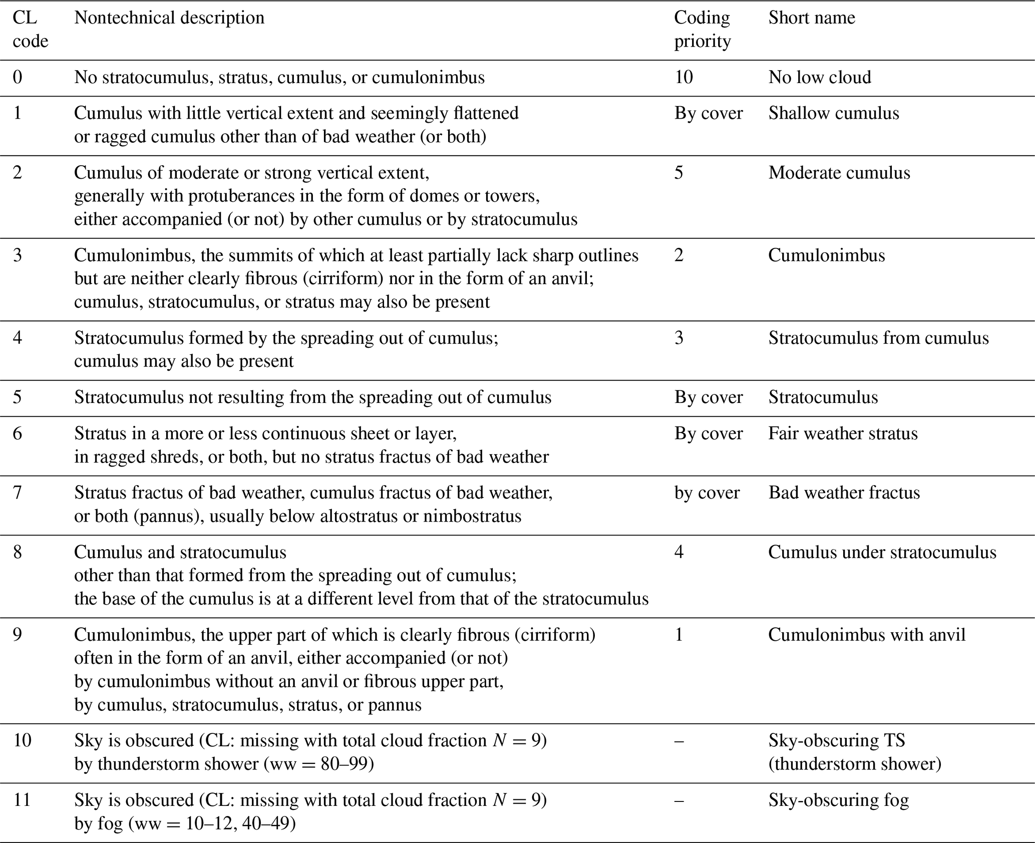
The surface observer reports cloud type (CL) and fractional area (LCA) of low-level clouds following a strict hierarchy from the World Meteorological Organization (WMO, 1975b. Table 1). In addition to the 10 CLs defined by the WMO, EECRA defines two more CLs (CL10, sky-obscuring thunderstorm and shower, and CL11, sky-obscuring fog) by combining the present weather code with the observation of missing CL. Consequently, an individual EECRA observation contains 12 CLs (from CL0 to CL11) and associated LCA (from 0 to 8 octas) such that a set of 12 CLs forms a complete basis function for the entire EECRA data. Based on similarities in morphology and physical property, we grouped individual CLs into eight groups: noCL (no low-level cloud), fog (sky-obscuring fog), F.St (fair weather stratus), B.St (bad weather stratus), Sc (stratocumulus), Sc–Cu (stratocumulus and cumulus), Cu (cumulus), and Cb (cumulonimbus), in approximately the increasing order of vertical instability (see Table 2). Since ELF is based on the decoupling hypothesis that can be applied in various regimes from the well-mixed to fully decoupled states, we included all CLs in our analysis. For individual CLs or combinations of CLs, we computed cloud frequency (FQ), amount when present (AWP), and amount (AMT), following the procedures described in Hahn and Warren (1999) and Park and Leovy (2004). Cloud FQ for a specific CL is defined by the fraction of observations reporting the specific CL among the total set of observations reporting any CL information. Cloud AWP is the average LCA when a specific CL is observed. Cloud AMT is the product of FQ and AWP.

Table 2Author-defined short names of low-level cloud (CL) types used in our study.

Download Print Version | Download XLSX

Similar to PS19, individual EECRA cloud observations, as well as surface and upper-level meteorologies are averaged into 5^∘ latitude × 10^∘ longitude seasonal data for each year. To reduce the impact of random noise, a minimum of 10 observations were required to form effective seasonal grid data in each year. These seasonal grid data are used for computing annual climatologies and seasonal differences of various CLs (Figs. 1–2) and analyzing correlations between the LCA and various proxies by cloud type (Tables 1–2 and Figs. 3–6). In addition, individual EECRA cloud observations are grouped into bins of individual proxies to better understand the contribution of individual CLs to the overall correlation relationship between the proxies and LCA (Figs. 7–8). ECTEI produced results very similar to those of EIS such that only the analysis for EIS is shown in this study.

3.1 Climatology and seasonal cycle

Figures 1 and 2 show the annual climatology and the differences in the seasonal FQ of various CLs during JJA and DJF. As shown, noCL is frequently observed over the continents but is rarely reported over the open ocean, implying that one of the important factors controlling the formation of low-level clouds is the moisture source at the surface. One of the rare open-ocean areas with annual noCL FQ larger than 10 % is the sea surface temperature (SST) cold tongue region in the eastern equatorial Pacific Ocean, where SST is lower than the overlying air temperature, net upward buoyancy flux from the sea surface is very weak, and the atmospheric PBL is stable (Deser and Wallace, 1990). As a result, turbulent vertical moisture transport from the sea surface to z_LCL is strongly suppressed (i.e., z_inv<z_LCL), resulting in the maximum FQ of noCL (Park and Leovy, 2004). This indicates that not only the moisture source at the surface, but also vertical stability in the atmospheric PBL controls the formation of low-level clouds. Over the continents and the Arctic area, noCL is more frequently observed during boreal winters than summers, presumably because strong daytime insolation during summer destabilizes the lower troposphere, promoting the onset of convective clouds (i.e., Sc–Cu, Cu, and Cb). Strong nocturnal LW radiative cooling during winter stabilizes the lower troposphere, which forces z_inv<z_LCL. In addition, the amount of moisture at the near surface is very small during winter. Similar to the case over the SST cold tongue, strong vertical stability over the winter continents and Arctic area appears to increase the probability of the occurrence of noCL, which appears to be somewhat opposite to the embedded decoupling processes into ELF that increases as z_inv decreases. However, with the freeze-dry factor, ELF may be able to capture enhanced noCL frequency over the continents during winter due to a small amount of moisture near the surface. PS19 showed that the freeze-dry factor substantially reduces ELF in this region during winter.

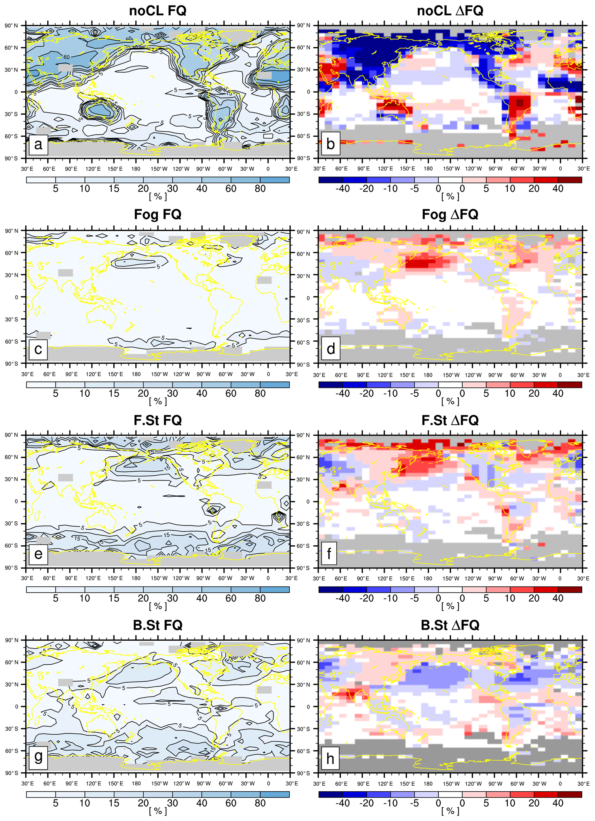
Figure 1(a, c, e, g) The annual mean climatological CL frequency (FQ) and (b, d, f, h) the differences in climatological CL FQ between JJA and DJF ($\mathrm{\Delta }\text{FQ}=\text{FQ(JJA)}-\text{FQ(DJF})$) for (a, b) noCL, (c, d) fog, (e, f) F.St, and (g, h) B.St. In the first column, the grid boxes with a total observation number less than 100 are shaded with gray. In the second column, statistically insignificant ΔFQ values at the 99.9 % confidence level from the two-sided Student's t test assuming independent samples are denoted by white, and the grid boxes with the observation number less than 100 during either JJA or DJF are shaded with gray.

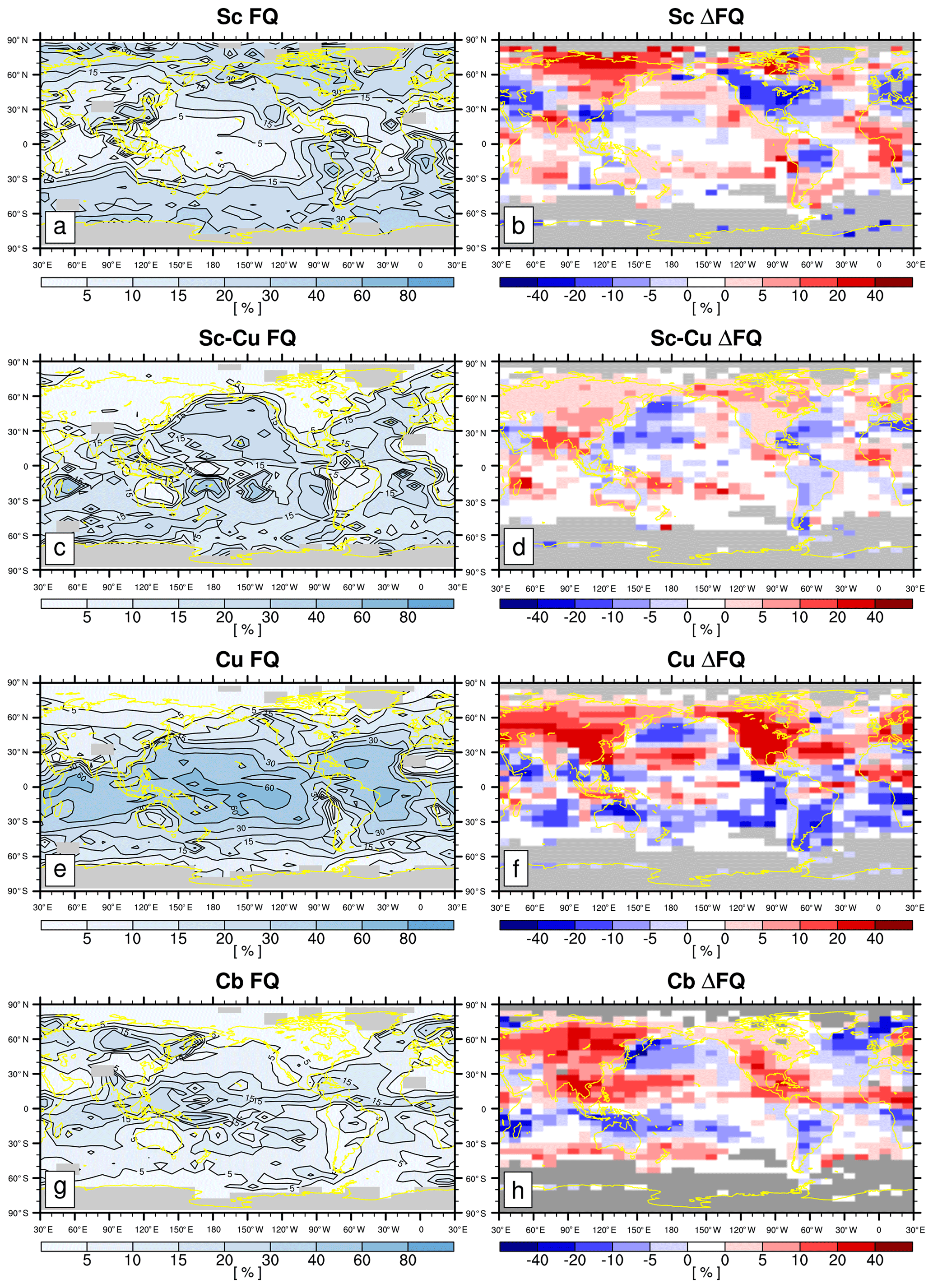
Figure 2Same as Fig. 1 but for Sc, Sc–Cu, Cu, and Cb.

Fog is frequently observed over the western North Pacific and Atlantic oceans, including the Arctic area, during JJA when the Arctic sea ice melts and moist warm air is advected into the cold SST region across the midlatitude SST front. This indicates the saturation of advected air parcels by the contact cooling with the underlying cold SST or more upward moisture transport from the open ocean over the Arctic, which can be captured by ELF through the decrease in z_LCL. F.St has a similar climatology and seasonal cycles as fog, implying that the physical processes controlling the formation of fog are similar to those of F.St. B.St has an annual climatology similar to that of F.St, but its seasonal cycle over the North Pacific and Atlantic oceans is opposite to that of F.St, with more frequency during boreal winters. Similar to B.St, Cb is more frequently observed during winter in this region, which is presumably due to the frequent passage of midlatitude synoptic storms in winter. A composite analysis showed that Cb is frequently observed on the rear side of the midlatitude synoptic cold front with a reduced lower tropospheric stability, while B.St is observed on the front or near center of the synoptic storm with an enhanced lower tropospheric stability (Houze, 2014; Park and Shin, 2020). When the midlatitude storm track passes, anomalous mean vertical motion in the mid-troposphere drives the changes in the mid-level clouds, but the variations in the lower tropospheric stability also drive the changes in LCA, which can be captured by ELF through the variations in z_inv.

In the Northern Hemisphere, Sc is frequently observed over the eastern subtropical and midlatitude oceans during JJA, when the subtropical and midlatitude high is strong and the PBL is relatively well coupled. In the Namibian and Peruvian stratocumulus decks west of South America and southern Africa, Sc is most frequently reported during SON when SST is at a minimum (Klein and Hartmann, 1993). Over most ocean areas, seasonal variations in Sc tend to be opposite to those of Cu and Cb. ELF is designed to capture these conversions between Sc and Cu in association with the PBL decoupling. Over northern Asia and Canada, including a portion of the Arctic area, both convective and stratiform clouds are more frequently observed during boreal summers than winters, presumably due to the destabilization of the lower troposphere by strong insolation heating and more surface moisture.

3.2 Proxy vs. the AWP of individual low-level clouds

Figures 3 and 4 show the composite anomalies of LCA and various proxies with respect to the seasonal climatology when a specific CL was reported (see Figs. S1 and S2 in the Supplement for the composite anomalies of z_LCL, z_inv, α, and 1−β₂). The anomalous LCA in the top row (ΔAWP) is the difference between the amount when present (AWP) when a specific CL was reported and climatological LCA. To examine the coherency between ΔAWP and the anomalies of individual proxies in each grid box, we computed the non-centered geographical correlation coefficients between ΔAWP and Δproxy over the entire globe (G), ocean (O), and land (L), respectively, which are shown at the top of the individual plots. Here, we used the non-centered correlations rather than centered correlations to assess whether the spatial means of ΔAWP and Δproxy, as well as the spatial variabilities of those, are similar.

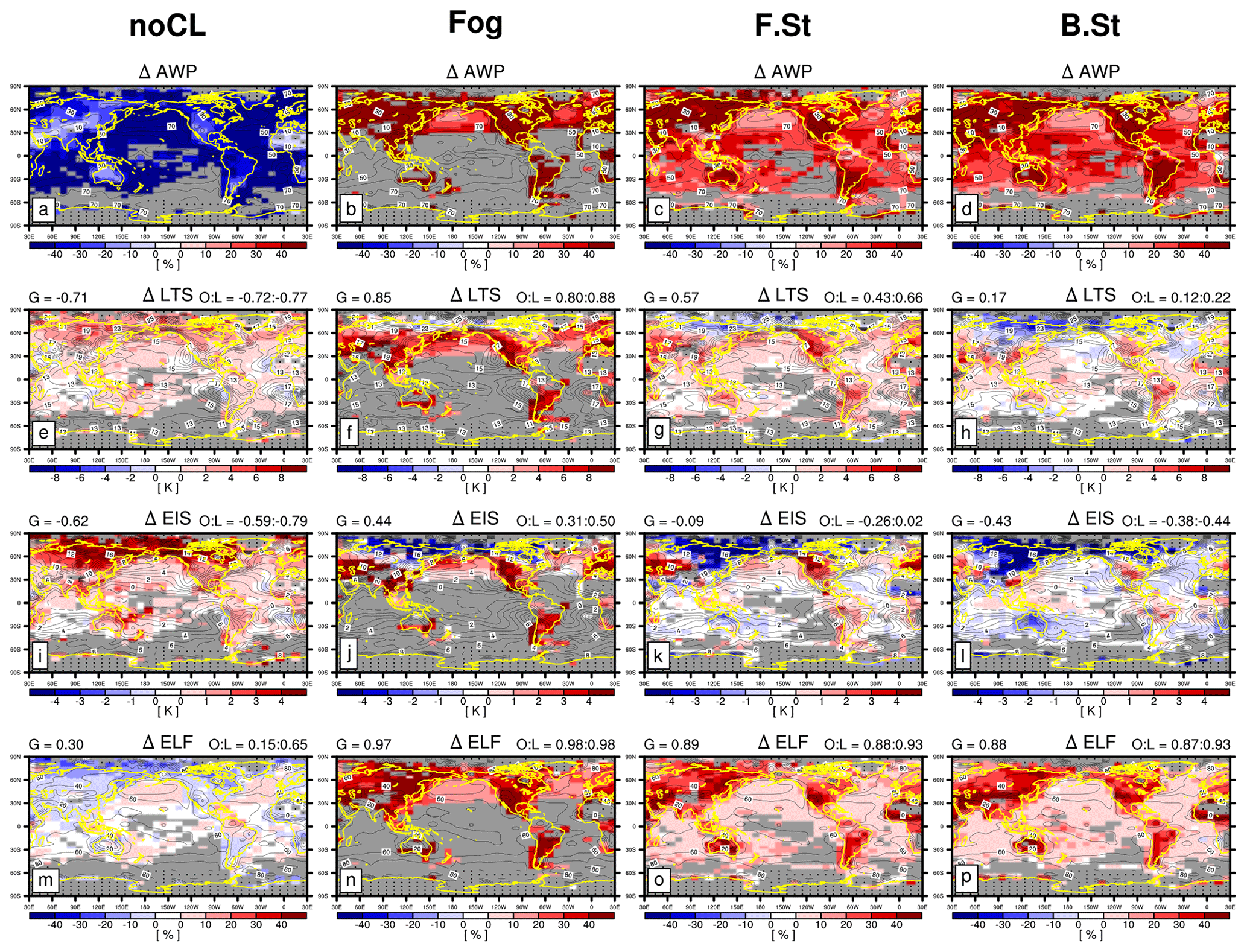
Figure 3Composite anomalies of (a–d) AWP (amount when present), (e–h) LTS, (i–l) EIS, and (m–p) ELF with respect to the annual climatology when (a, e, i, m) noCL, (b, f, j, n) fog, (c, g, k, o) F.St, and (d, h, l, p) B.St were reported. ΔAWP is the difference between the AWP of a specific CL and climatological LCA. The contour line is the annual climatology of LCA and individual proxies. At the top of individual plots, non-centered correlation coefficients between ΔAWP and Δproxy over the globe (G), ocean (O), and land (L) are shown. In each plot, statistically insignificant anomalies at the 99.9 % confidence level from the two-sided Student's t test assuming independent samples are denoted by white, and grid boxes with the observation number of a specific CL less than 100 are shaded by gray. Grid boxes with a total observation number less than 100 are marked with a dot.

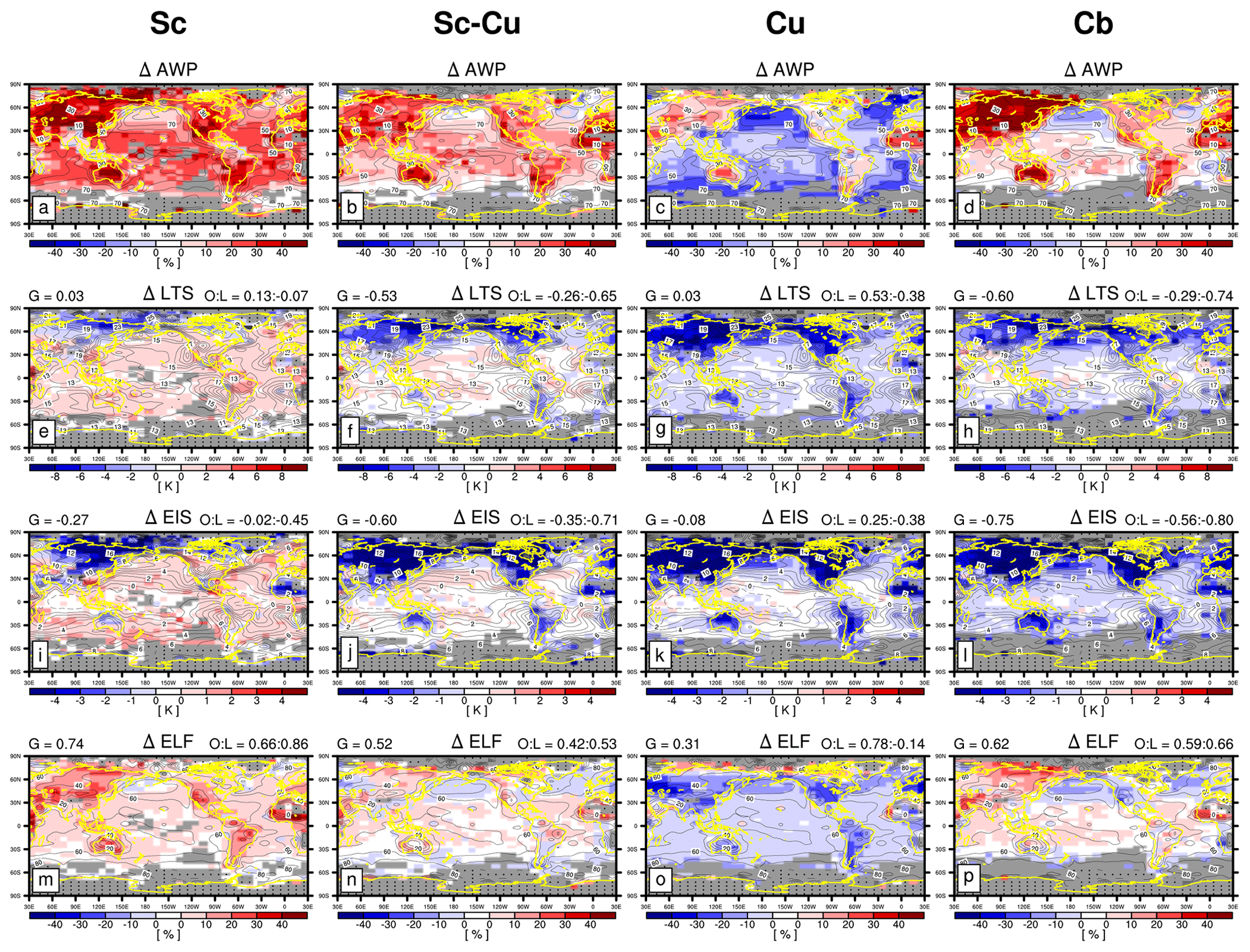
Figure 4Same as Fig. 3 but for Sc, Sc–Cu, Cu, and Cb.

When noCL is reported, AWP is zero, that is, $\mathrm{\Delta }\text{AWP}=-\text{LCA}$ in Fig. 3a. However, both LTS and EIS increase ($\mathrm{G}=-\mathrm{0.714}$ and −0.62 for LTS and EIS, respectively), particularly over the far northern continents and Arctic area. This is because noCL can occur when inversion is strong near the surface under dry conditions (Norris, 1998; Koshiro and Shiotani, 2014). Conversely, ELF decreases in a desirable way due to the freeze-dry factor (compare Fig. 3m with Fig. S1m). Over the eastern subtropical marine stratocumulus deck, LTS, EIS, and ELF show a hint of negative anomaly which, however, is too weak to explain the substantial decrease in LCA when noCL is reported. Over the midlatitude oceans, the situation is worse and none of the factors comprising ELF (i.e., z_LCL, z_inv, and α) can explain the decrease in LCA (Fig. S1a, e, i). Although slightly better than LTS and EIS, ELF has an apparent problem in diagnosing the decrease in LCA when noCL was reported, particularly over the ocean (O=0.15). This problem worsens without the freeze-dry factor (Fig. S1m). When fog, F.St, or B.St are reported, LCA increases over the entire globe, which is very well captured by ELF (G=0.97, 0.89, and 0.88 for fog, F.St, and B.St, respectively), due to the simultaneous decreases in z_LCL, z_inv, and α. Although slightly worse than ELF, LTS and EIS also capture the increase in LCA when fog was reported (G=0.85 and 0.44 for LTS and EIS, respectively). However, undesirable negative anomalies of LTS and EIS over the far northern continents, including the Arctic area, worsen from fog to F.St and B.St, resulting in very weak (G=0.17 for LTS) or even negative ($\mathrm{G}=-\mathrm{0.43}$ for EIS) correlations between ΔLTS–ΔEIS and ΔAWP when B.St was reported. We speculate that in these dry regions, the formation of fog, F.St, and B.St needs upward moisture transports from the surface, which is likely to be accompanied by the reduction of vertical stability in the lower troposphere (e.g., breakup of sea ice over the Arctic). As a result, ΔLTS and ΔEIS are negatively correlated with ΔAWP over the far northern continents and Arctic area. Overall, ELF is better than LTS and EIS in diagnosing the variations of fog and stratus over both the ocean and land. It should be noted that LTS, EIS, and ECTEI are mainly designed to be used over the ocean without sea ice, and they are not intended to be used over land and sea ice.

In addition to the fog and stratus, ELF captures the variations in LCA in association with Sc (G=0.74), Sc–Cu (G=0.52), Cu (G=0.31), and Cb (G=0.62) reasonably better than LTS and EIS. When Sc was reported and LCA increases, both LTS and EIS increase over the subtropical and midlatitude oceans. However, over the Arctic, Asia, and deserts areas, LTS and EIS show negative anomalies opposite to the increased LCA, which worsens and extends to other continents from Sc and Sc–Cu to Cu and Cb, resulting in substantial negative correlations between ΔLTS–ΔEIS and ΔLCA over land for Sc–Cu ($\mathrm{L}=-\mathrm{0.65}/-\mathrm{0.71}$ for LTS and EIS), Cu ($\mathrm{L}=-\mathrm{0.38}/-\mathrm{0.38}$), and Cb ($\mathrm{L}=-\mathrm{0.74}/-\mathrm{0.80}$). The negative correlation for Sc can be explained by the same physical processes applied to the cases of fog, F.St, and B.St as explained above (i.e., enhanced moisture transport from the surface and associated decrease in vertical static stability). In the very dry regions where background LCA is very small, the onset of Cu and Cb in unstable situations (e.g., decreases in LTS and EIS) will result in the increase in LCA. Although generally better than LTS and EIS, ELF also has a problem in capturing the increase in LCA over Asia and most desert areas when Cu was reported ($\mathrm{L}=-\mathrm{0.14}$). In summary, an advanced ELF in the future should be designed to capture the decrease in maritime LCA associated with noCL and the increase in continental LCA associated with Cu.

Figure 5Seasonal climatologies of the (a, b) AWP, (c, d) LTS, (e, f) EIS, and (g, h) ELF averaged over the (left) ocean and (right) land for each season (DJF, MAM, JJA, and SON, denoted by different colors) during the daytime (09:00–21:00, upward bars with bright colors) and nighttime (21:00–09:00, downward bars with dark colors) when a specific CL was reported. In each plot, CLM denotes the climatology for all CLs.

Download

Figure 5 shows the area-averaged seasonal climatology of the AWP and various proxies when a specific CL was reported over the ocean and land during the daytime (09:00–21:00) and nighttime (21:00–09:00), respectively (see Fig. S3 for z_LCL, z_inv, α, and 1−β₂). By definition, fog is always overcast, and stratiform clouds tend to have larger AWP than convective clouds. Cb has larger AWP than Cu, presumably due to larger cross-sectional and lateral areas of deep convective updraft plumes or the contribution of detrained convective condensates. With the exception of Cb, AWP over the ocean is slightly larger than that over land. The diurnal cycle of the AWP in most CLs is very weak. However, continental Cb during the night tends to have a slightly larger AWP than during the day, which seems to be contradictory to the intuition that deep cumulonimbus over land is forced by strong insolation heating during the day. This may reflect the late evening or nocturnal development of the strongest deep convective system over the continents in association with the gradual buildup of the mesoscale convective organization forced by the evaporation of convective precipitation (Park, 2014a, b). As a global proxy for the AWP of individual CLs, ELF shows more desirable inter-CL variations than LTS and EIS, which have strong ocean–land contrasts (in particular, EIS) and a seasonal cycle over land. The weaker seasonal cycle and ocean–land contrasts of ELF may imply opposite variations in z_inv and z_LCL. Due to the freeze-dry factor, ELF is slightly smaller than 1−β₂ during DJF over land, and the freeze-dry factor also contributes to reducing the excessive seasonal cycle (compare Figs. 5h and S3h). ELF has a somewhat stronger diurnal cycle than AWP over land with a larger ELF during the night, which is presumably due in part to diagnosing the noCL condition as a nonzero ELF, as will be explained later. The factors comprising ELF (z_LCL, z_inv, and α) have fairly similar inter-CL variations, with larger values for convective than stratiform clouds (Fig. S3). Interestingly, z_LCL for Cb is smaller than that of Cu, presumably due in part to the evaporation of convective precipitation and the associated moistening and latent cooling of near-surface air when Cb was reported.

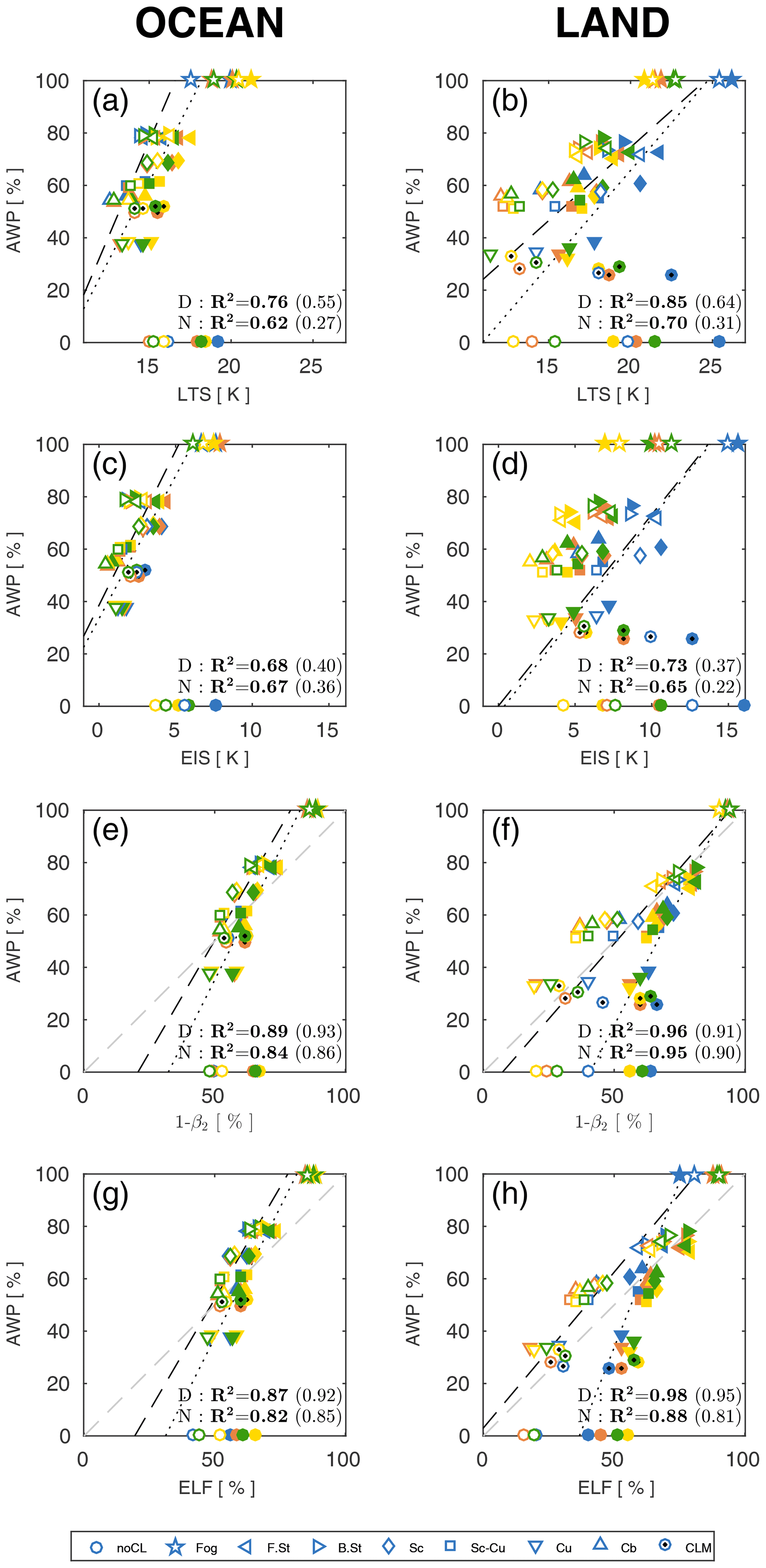
Figure 6Scatter plots of Fig. 5 over the (a, c, e, g) ocean and (b, d, f, h) land during the daytime (open symbols) and nighttime (filled symbols). Also plotted are the linear regression lines and squared correlation coefficients (R²) during the daytime (D, dashed) and nighttime (N, dotted). The bold R² values are when CLM and noCL are excluded in the regression analysis, and the R² values in parenthesis are when fog is additionally excluded. The seasons are marked with the same colors as Fig. 5. The dashed gray lines in the last four plots denote AWP = ELF.

Download

Figure 6 shows the scatter plots of individual CL AWP as a function of LTS, EIS, 1-β₂, and ELF obtained from Fig. 5. If noCL is excluded, all proxies have very good correlations with the AWP of individual CLs, although ELF and 1−β₂ perform slightly better than LTS and EIS. If fog is also excluded, the correlations between LTS–EIS and AWP are substantially degraded, whereas the performances of ELF and 1−β₂ do not change much (see R² in parenthesis in Fig. 6). Similar to the regression analysis of PS19, the slope of inter-CL AWP regressed on ELF during the day over the ocean is steeper than that over land. Over the ocean, the regression slopes during the night are roughly similar to those during the day but with systematically higher proxy values. For all cloud types, ELF during the night tends to be larger than during the day, particularly over land, indicating that the product of z_inv and z_LCL during the day is larger than during the night. This is an anticipated result since shortwave radiative heating of the surface during the day destabilizes the lower troposphere (i.e., increases z_inv) and decreases the relative humidity of the near-surface air (i.e., increases z_LCL). Over land, however, both ELF and 1−β₂ tend to have steeper regression slopes during the night than during the day. This is due in part to the diagnosis of the noCL condition as a nonzero ELF, particularly during the night, when noCL conditions are frequently reported (see Fig. 1a). To be a better proxy for LCA (i.e., LCA = ELF denoted by the dashed gray line), ELF of noCL (and Cu except over land during the day) should be much lower than the current values, while the ELFs of Sc, Sc–Cu, Cb, and Cu over land during the day as well as fog, F.St, and B.St over the ocean should be higher than the current values. These required behaviors are fairly consistent with the conclusion drawn from the analysis of Figs. 3 and 4. In contrast to previous studies reporting a superior performance of EIS compared to LTS, our analysis does not show a clear difference in their performances. This is presumably because our study compared their performances over the entire globe instead of marine stratocumulus decks, the main target areas of EIS and LTS.

3.3 Proxy vs. the FQ of individual low-level clouds

Figure 7 shows stacked percentage plots of the frequencies of individual CLs in the bins of various proxies, defined as the number of observations reporting a specific CL divided by the total observation number in each bin. Figure 7a, a plot with a perfect proxy for LCA, shows that noCL exists entirely in the 0 octa bin, fog only exists in the 8 octa bin, and the bin AWP (black line) increases in a perfect linear way as LCA increases, as expected. As LCA increases, the frequency of Cu decreases but that of stratiform clouds (F.St, B.St, Sc, and Sc–Cu) tends to increase. In contrast to Cu, the frequency of Cb in the low octa bins gradually increases with LCA. The observation number is relatively large in the 0 and 8 octa bins (yellow line). The low-level cloud AMT contributed by individual bins (the cyan line that is a simple product of the black and yellow lines) increases with LCA but not in a perfectly linear way. The overall patterns over land are approximately similar to those over the ocean. Over land, the observation number is the largest in the 0 octa bin, and convective clouds (Cu and Cb) are mostly observed during the day. Any good proxy for LCA, if there is one, should have similar patterns as Fig. 7a and b.

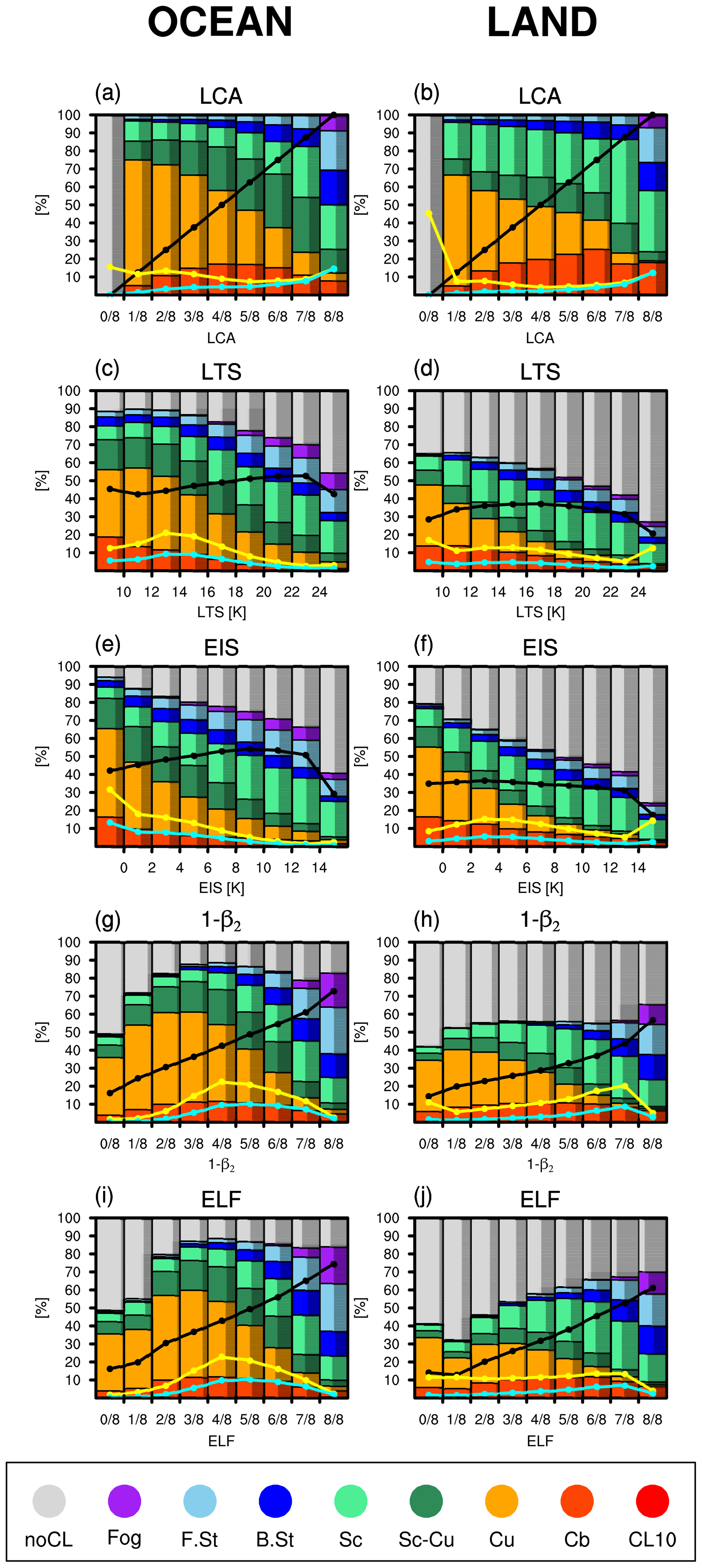
Figure 7Stacked percentage plots for the FQs of individual CLs in the bins of various proxies: (a, b) LCA (i.e., a perfect proxy for LCA), (c, d) LTS, (e, f) EIS, (g, h) 1-β₂, and (i, j) ELF over the (left) ocean and (right) land. AWP of all CLs in each bin is denoted by the black line. The observation number FQ of individual bins (the ratio of the observation number in each bin to the total observation number of entire bins) is denoted by the yellow line. LCA in each bin is denoted by the cyan line, which is the product of the black and yellow lines. The sum of the yellow line integrated over the entire bins is 100 %. The sum of the cyan line integrated over the entire bins is the global annual mean LCA. The bright and dark colors in each bar denote the fractions during the daytime and nighttime, respectively.

Download

The frequency of noCL increases as LTS and EIS increase, which is mainly responsible for the undesirable decreases in the AWP and AMT in the high bins of LTS and EIS. Designed as a proxy for marine stratocumulus, however, LTS and EIS reasonably simulate the increase (decrease) in Sc (Cu) frequency with LTS and EIS over the ocean. The increase in noCL frequency with LTS and EIS seems to be contradictory to our simple intuition that LTS and EIS are positively correlated with LCA. However, we note that the noCL condition is frequently reported with a strong inversion near the surface when LTS and EIS are large (Norris, 1998; Koshiro and Shiotani, 2014). Note that the implied correlation between LCA and EIS in Fig. 7e is weaker than in previous studies (Wood and Bretherton, 2006), since LCA in Fig. 7 is defined by including all low-level cloud types over the globe. In contrast to the case of LCA, fog exists in several bins, and the frequency of Cb decreases monotonically with LTS and EIS. Similar to the case of LTS and EIS, noCL exists ubiquitously in the entire ELF bins, indicating that the observed noCL conditions are frequently misinterpreted as cloudy conditions with LTS, EIS, and ELF. However, the frequency of noCL tends to decrease with ELF such that the bin AWP increases in a desirable way as ELF increases, although the slope is smaller than the case of LCA. The frequency of noCL in the nonzero ELF bins over land is substantially higher than that over the ocean. The observation number FQs in the 0 and 8 octa ELF bins are substantially lower than those in the LCA bins but higher in the intermediate bins, implying that an advanced ELF needs to transfer the observation number FQ in the intermediate ELF bins into the 0 octa bin (e.g., by correctly diagnosing a noCL condition) and 8 octa bin (e.g., by correctly diagnosing a fog condition).

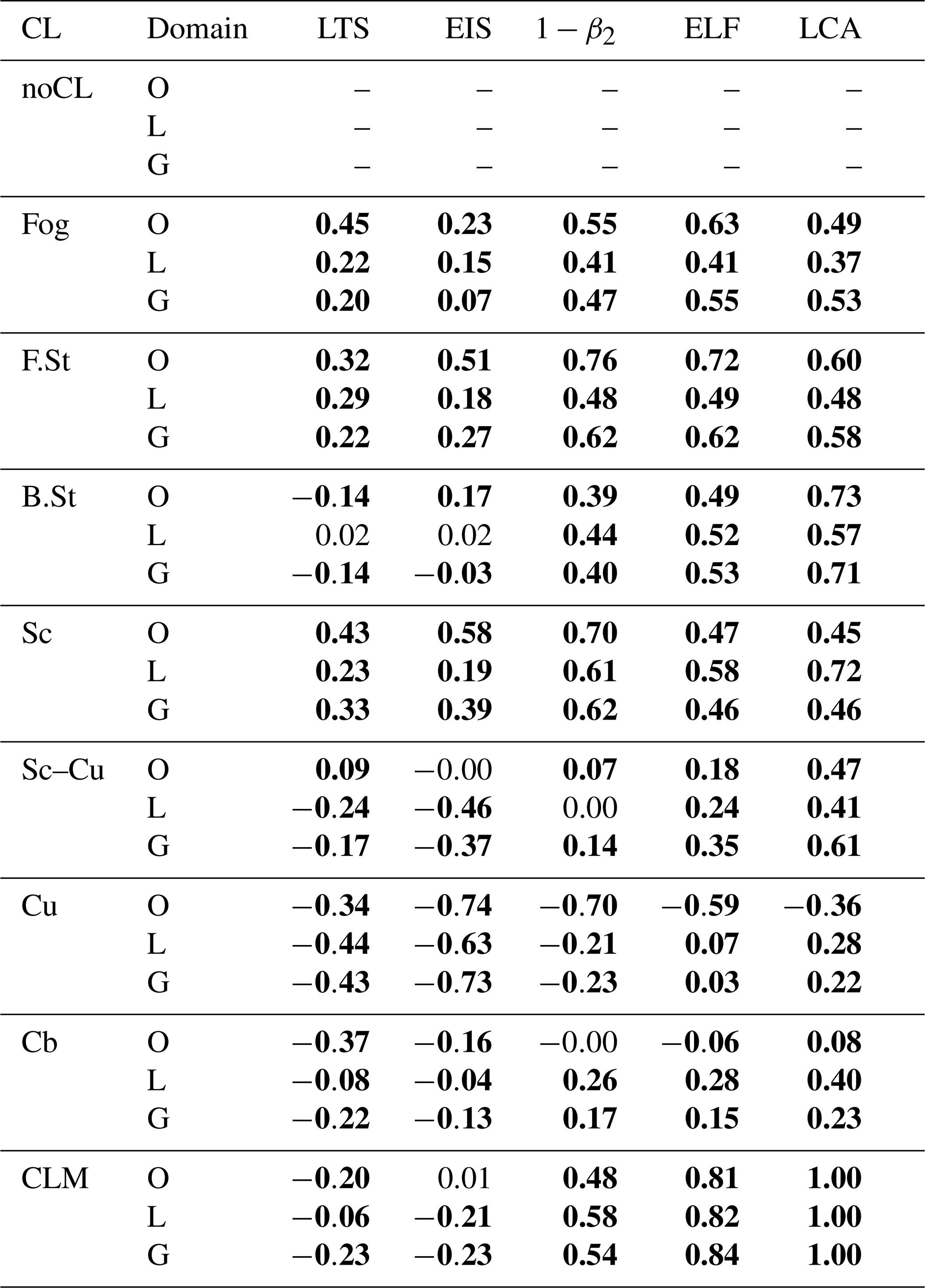
Table 3 shows spatial–seasonal correlation coefficients between the frequency of individual CLs and various proxies. In contrast to Figs. 3 and 4, Table 3 (also Table 4) shows a conventional centered correlation between the seasonal climatologies (i.e., averaged over all observations) of various proxies and individual CL frequency. LCA increases as the frequencies of sky-obscuring fog (fog), stratus (F.St, B.St), stratocumulus (Sc, Sc–Cu), and continental convective clouds (Cu, Cb) increase, and it decreases as the frequencies of noCL and marine convective clouds increase. Except for marine Sc–Cu and continental Cu, ELF reproduces these correlation characteristics of LCA with individual CLs well, at least qualitatively. The freeze-dry factor substantially contributes to the improved correlations of noCL with ELF from β₂. As explained in PS19, the freeze-dry factor ($f=\text{max}[\mathrm{0.15},\text{min}(\mathrm{1},q_{\mathrm{v},\text{sfc}}/\mathrm{0.003}\left)\right]$) is designed to reduce a diagnosed LCA in a very dry region such that it is most effective over the far northern continents and Arctic area, particularly during winter. Over the globe, noCL is negatively correlated with z_inv and α (not shown), presumably due in part to the frequent occurrence of noCL on the west coast of the major continents and the equatorial SST cold tongue regions where z_inv is low due to cold SST (see Fig. 1a). The frequent occurrence of noCL on the west coast is due to the advection of dry air from nearby continents (Mansbach and Norris, 2007). The frequent occurrence of noCL over the SST cold tongue is due to warm air advection from the south, the associated stabilization of the lower PBL, and the suppression of vertical moisture transport from the sea surface to z_LCL (Park and Leovy, 2004). Designed as proxies for marine stratocumulus, LTS and EIS show a strong correlation with Sc FQ over the ocean. However, the correlation characteristics of LTS and EIS with other CLs are less desirable than that of ELF. For example, the correlations of LTS and EIS with fog, F.St, and B.St over the globe and continental Sc are significantly weaker than those of LCA, and the correlation signs with noCL, Sc–Cu, and continental Cu and Cb are opposite to those of ELF and LCA. One of the most unexpected aspects of LTS and EIS is a strong positive correlation with noCL FQ, as shown in Fig. 7. This may indicate a nonlinear response of clouds to the inversion strength or the existence of other factors controlling the onset of noCL condition.

Table 3Spatial–seasonal correlation coefficients between various proxies and the frequency (FQ) of individual CLs. In contrast to Figs. 3 and 4 where non-centered correlation coefficients were computed, the values in this table are the conventional centered correlation coefficients computed from the climatological seasonal proxies obtained by using all observations in each seasonal grid box instead of the observations reporting a specific CL. In this table, LCA is a perfect proxy for LCA. Statistically significant correlations at the 99.9 % confidence level from the Student's t test assuming independent samples are denoted by bold.

Download Print Version | Download XLSX

Table 4Same as Table 3 but for the amount (AMT) of individual CLs.

Download Print Version | Download XLSX

3.4 Proxy vs. the AMT of individual low-level clouds

Figure 8 shows stacked plots of the AMT of individual CLs in the bins of various proxies. The LCA is the AMT of all CLs. The bin cloud AMT (the cyan line) increases monotonically with LCA, with the largest increase from the 7 to 8 octa bin (Fig. 8a, b). In the low bins, convective clouds contribute to the cloud AMT more than stratiform clouds, but in the high bins, stratiform clouds contribute more. Total cloud AMT (i.e., the integration of the cyan line across the entire bins) over the ocean is larger than that over land. In the 8 octa bin over land, Cb contributes more than 20 % to the cloud AMT. In contrast to LCA, none of the proxies show a required monotonic increase in the bin cloud AMT. Over the ocean, EIS shows an undesirable monotonic decrease in the bin cloud AMT, LTS is slightly better than EIS, and ELF shows a further improvement, with the maximum bin cloud AMT shifting to the higher bin. The improvement from EIS and LTS to ELF is more pronounced over land, but the rapid decrease in bin cloud AMT from the 7 to 8 octa ELF bins is problematic. These variations in the bin cloud AMT are largely controlled by the variations in the bin cloud FQ (see the yellow line in Fig. 7). All proxies show the increase in the relative contribution of stratiform clouds to the bin cloud AMT as the bin value increases, but the contribution of Cb AMT in the 8 octa bin over land is smaller than that of LCA.

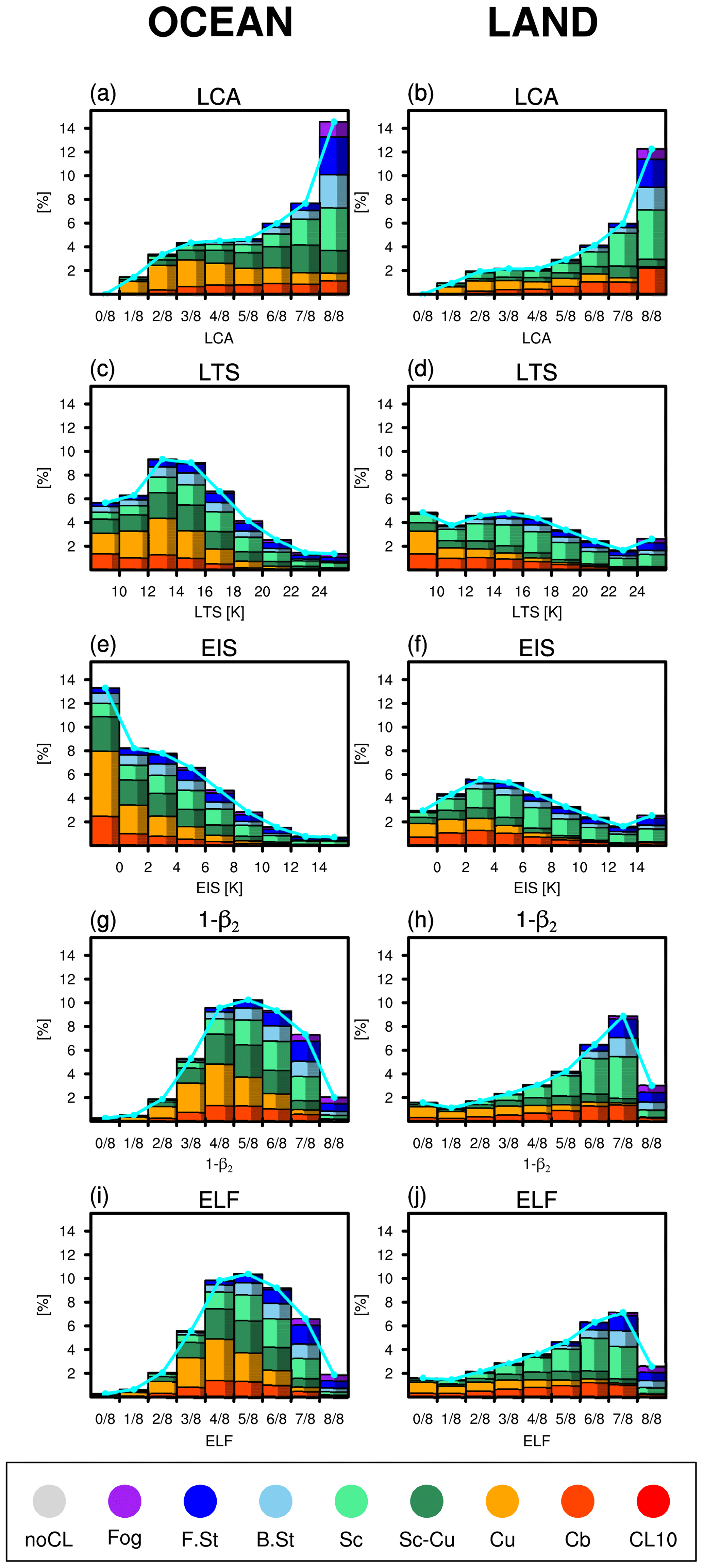
Figure 8Same as Fig. 7 but for the AMT of individual CLs in each bin. The cyan lines are identical to those shown in Fig. 7. The sum of all CL AMTs integrated over the entire bins is the global annual mean LCA, which is identical regardless of the proxies used for the composite.

Download

Table 4 shows spatial–seasonal correlation coefficients between the AMT of individual CLs and various proxies. The overall correlation characteristics of the cloud AMT are very similar to those of the cloud FQ shown in Table 3. LCA tends to increase as the cloud AMT of individual CLs increases. The only exception is marine Cu AMT that decreases as LCA increases. ELF reproduces these correlation characteristics of the AMT of individual CLs with LCA well. As a global proxy for LCA, the correlation characteristics of LTS and EIS with individual cloud AMT are less desirable than those of ELF: the correlations with continental Cu and Sc–Cu are unrealistically negative, and the correlations with sky-obscuring fog and stratus are much weaker than those of ELF and LCA. We note that LTS, EIS, and ECTEI are designed to be used over the ocean without sea ice, and they are not intended to be used over land and sea ice. Table 4 indicates that a superior performance of ELF compared to LTS and EIS as a global proxy for LCA discovered by PS19 (see the bottom row of Table 4) is derived from its realistic correlations with various CLs rather than with a specific CL.

3.5 What is necessary to further improve ELF as a global proxy for LCA?

We have shown that, generally, ELF diagnoses the inter-CL variations in LCA better than LTS and EIS. However, we also identified several weaknesses in ELF, such as the increase in ELF over the ocean when noCL was reported and the decrease in ELF over deserts and Asian continents when Cu was reported and LCA increases. In this section, we examine in more detail why ELF shows undesirable correlations with LCA for some cases and then provide a potential pathway to further improve ELF in the future.

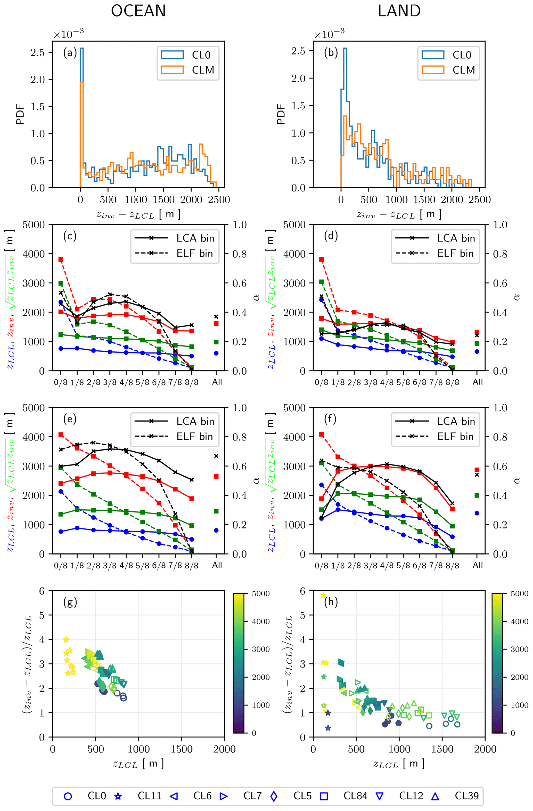
Figure 9(a, b) Probability density functions (PDFs) of $z_{\text{DL}}=z_{\text{inv}}-z_{\text{LCL}}$ when noCL was reported (blue) and any CL was reported (red); (c–f) z_LCL (blue), z_inv (red), α (black), and $\sqrt{z_{\text{LCL}}\cdot z_{\text{inv}}}$ (green) in each octa bin of LCA (solid lines) and ELF (dashed lines) when (c, d) Sc was reported and (e, f) Cu was reported, with the values averaged over the entire bins denoted by “all” in the right column. (g, h) The distribution of $\mathrm{\Delta }{z}_{\mathrm{s},i}=\left(\sqrt{z_{\text{inv}}\cdot z_{\text{LCL}}}\right)/(\mathrm{1}-\text{AWP}/f)$ (shaded; in meters) as a function of z_LCL and $\mathit{\delta }\equiv z_{\text{DL}}/z_{\text{LCL}}$ for individual data points shown in Fig. 6g and h. The plots in the left and right columns are over the ocean and land, respectively.

Download

When noCL is reported, ELF increases over the North Pacific and North Atlantic oceans, which results in a very weak non-centered correlation over the ocean (O=0.15) between ΔLCA (Fig. 3a) and ΔELF (Fig. 3m). Although the correlation over land (L=0.65) is higher than over the ocean, the magnitude of ΔELF is much smaller than ΔLCA. As shown in Fig. 6g and h, noCL is the most distinct outlier from the desirable AWP = ELF line (dashed lines) in the inter-CL scatter plots. This misdiagnosis of the noCL condition with nonzero ELF is also shown in Fig. 7i and j, and it worsens over land during the night. To understand this problem, we plotted the probability density function (PDF) of $z_{\text{DL}}\equiv z_{\text{inv}}-z_{\text{LCL}}$ using individual observations reporting noCL and compared it with the PDF of entire observations (CLM) over the ocean (Fig. 9a) and land (Fig. 9b). As shown, the PDF of near-zero z_DL when noCL was reported is higher than that of CLM, and the difference over land is larger than that over the ocean. Conceptually, if z_DL<0 and so z_inv<z_LCL, low-level cloud cannot be formed such that LCA is likely to be small. This can happen when dry air at the surface is capped by a strong inversion such that vertical moisture transport from the surface to z_LCL is inhibited. However, since our $\text{ELF}=f\cdot (\mathrm{1}-\sqrt{z_{\text{inv}}\cdot z_{\text{LCL}}}/\mathrm{\Delta }{z}_{\mathrm{s}})=f\cdot [\mathrm{1}-(z_{\text{LCL}}/\mathrm{\Delta }{z}_{\mathrm{s}}\left)\sqrt{\mathrm{1}+z_{\text{DL}}/z_{\text{LCL}}}\right]$ is formulated as a function of $z_{\text{inv}}=\text{max}(z_{\text{inv}}^{*},z_{\text{LCL}})$ instead of $z_{\text{inv}}^{*}$ (where $z_{\text{inv}}^{*}$ is the inversion height directly obtained from Eq. (5) without any clipping such that $z_{\text{inv}}^{*}$ can be lower than z_LCL), this case of $z_{\text{inv}}^{*}<z_{\text{LCL}}$ is diagnosed as a highly cloudy condition in the current ELF. It seems that an advanced ELF needs to be able to simulate the decrease in LCA with the increase in the absolute value of $z_{\text{DL}}^{*}\equiv z_{\text{inv}}^{*}-z_{\text{LCL}}$, such as $\text{ELF}=f\cdot [\mathrm{1}-(z_{\text{LCL}}/\mathrm{\Delta }{z}_{\mathrm{s}}\left)\sqrt{\mathrm{1}+a\cdot {\mathit{\delta }}_{*}^{\mathrm{2}}}\right]$, where ${\mathit{\delta }}_{*}\equiv z_{\text{DL}}^{*}/z_{\text{LCL}}$ is a generalized decoupling parameter and a is a positive constant. This approach is likely to relocate the observation frequency of noCL in the high ELF bins into the low ELF bins (Fig. 7i and j), reduce the large ELF values for noCL (Fig. 6g and h), and improve the non-centered correlations between ΔELF and ΔLCA for various CLs including noCL (Figs. 3 and 4).

Another apparent problem of the current ELF is the decrease in ELF over desert areas (e.g., Sahara, Australia, and Saudi Arabia) when Cu was reported (see Fig. 4c and o). In contrast to the ocean where the onset of Cu is often associated with the decoupling of the PBL and decreases in overlying marine stratocumulus and LCA (e.g., Bretherton, 1992; Park et al., 2004), the onset of Cu over deserts without the background stratocumulus seems to directly increase LCA. In this case, ELF tries to mimic the observed increase in LCA by decreasing LCL (see Fig. S2c), but the larger increases in z_inv and associated PBL decoupling seem to offset the impact of the reduced LCL, resulting in the decrease in ELF. Conceptually, the current ELF is designed to mainly diagnose the variations in stratiform clouds and detrained cumulus at the inversion base, not the cumulus updraft plume itself (see Fig. 1 of PS19), which is reflected in part by the higher non-centered correlations between ΔELF and ΔAWP for stratiform clouds than for convective clouds as shown in Figs. 3 and 4. To further improve the performance of ELF, it seems to be necessary to additionally diagnose the fraction of cumulus updraft plume, particularly in regions without background stratiform clouds, such as deserts. Because the onset of Cu is closely associated with the PBL decoupling, one plausible approach is to incorporate a process to increase ELF as δ_* increases such that it can offset the decreases in stratocumulus and ELF with increasing δ_*. If the aforementioned $\text{ELF}=f\cdot [\mathrm{1}-(z_{\text{LCL}}/\mathrm{\Delta }{z}_{\mathrm{s}}\left)\sqrt{\mathrm{1}+a\cdot {\mathit{\delta }}_{*}^{\mathrm{2}}}\right]$ is adopted as an advanced ELF, the contribution of the cumulus updraft plume can be incorporated by setting a to be smaller (or even negative) than the default case, excluding the contribution of the cumulus updraft plume. Potentially, a could be parameterized as a decreasing function of z_LCL.

Figure 9c–f show the variations in z_LCL, z_inv, $\sqrt{z_{\text{LCL}}\cdot z_{\text{inv}}}$, and α as a function of ELF and LCA when Sc and Cu were reported over the ocean and land, respectively. When averaged over the entire bins (the “all” bin in the right column in each plot), Cu has higher z_LCL, z_inv, and α than Sc, which is consistent with our conceptual understanding. The increase in Cu AWP from the 0 to 1 octa bin over land is accompanied by the rapid increase in α (black solid line in Fig. 9f), presumably reflecting the onset of the cumulus updraft plume as the PBL is decoupled, which, as mentioned before, is not correctly captured by the current ELF (black dotted line in Fig. 9f). For both Sc and Cu (and also other CLs; not shown), z_LCL tends to decrease monotonically with LCA and ELF; however, z_LCL and z_inv decrease more rapidly with ELF than with LCA. As a result, the decreasing rate of $\sqrt{z_{\text{inv}}\cdot z_{\text{LCL}}}$ with ELF is much larger than that with AWP (green lines in Fig. 9c–f). One simple way to remedy this problem is to parameterize the scale height Δz_s in $\text{ELF}=f\cdot (\mathrm{1}-\sqrt{z_{\text{inv}}\cdot z_{\text{LCL}}}/\mathrm{\Delta }{z}_{\mathrm{s}})$ as a function of appropriate environmental variables, such as z_inv, z_LCL, and q_v,sfc. To check whether this is a possible approach, we computed an ideal scale height Δz_s,i in an ad hoc manner such that it exactly reproduces the observed LCA. More specifically, for individual data points shown in Fig. 6g and h, we computed $\mathrm{\Delta }{z}_{\mathrm{s},i}=\left(\sqrt{z_{\text{inv}}\cdot z_{\text{LCL}}}\right)/(\mathrm{1}-\text{AWP}/f)$ by inverting Eq. (4) (here, we implicitly assumed that Δz_s used in Eq. (4) for deriving ELF differs from Δz_s=2750 m used in Eq. (5) for deriving z_inv, which is a completely reasonable assumption because there is no physical reason for Δz_s in both equations to be identical). Figure 9g and h show the distribution of Δz_s,i in the phase space of z_LCL and $\mathit{\delta }\equiv z_{\text{DL}}/z_{\text{LCL}}$ over the ocean and land, respectively. As shown, Δz_s,i has a large inter-CL spread (and also relatively smaller seasonal and diurnal spreads) instead of being a constant 2750 m. There is a tendency for fog and stratus to have larger Δz_s,i than noCL and convective clouds, and to the first order, Δz_s,i seems to increase as δ increases and z_LCL decreases. Various CLs, each of which have their own distinct PBL structure and AWP, seem to be reasonably separated from each other in this phase diagram, implying a possibility to parameterize Δz_s as a function of z_LCL and δ. Because an advanced ELF needs to incorporate other aspects discussed in the above two paragraphs, which will presumably involve some changes in the functional form of ELF, we leave a detailed parameterization of Δz_s for future research.