2.1 Model description and set-up

ADMS-Urban, developed by Cambridge Environmental Research Consultants (CERC), is a quasi-Gaussian pollution dispersion and chemistry model that has been applied worldwide for environmental regulation, investigation and assessment of emission control strategies and generation of high spatial resolution air quality forecasts (McHugh et al., 2005; Carruthers, 2009; Cai and Xie, 2011).

The model domain (75 km×90 km) covers urban Beijing, defined here as everywhere within the Sixth Ring Road (marked in Fig. 1), and extends into the suburban counties of Shunyi and Changping to the north and Tongzhou, Daxing and Fangshan to the south, as illustrated by Fig. 1.

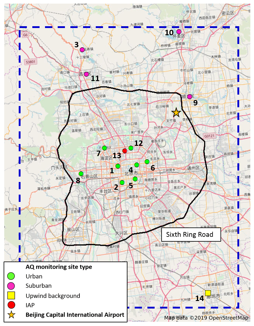
Figure 1Map of Beijing (source: OpenStreetMap, 2019) with the modelling domain, measuring 75 km×90 km, outlined (dashed blue line). Urban (green circle), suburban (pink circle), upwind background (yellow square) and IAP (red circle) air quality monitoring station locations, including site numbers, are provided. Beijing Capital International Airport (yellow star) and the Sixth Ring Road (black line) are also highlighted. © OpenStreetMap contributors 2019. Distributed under a Creative Commons BY-SA License.

2.1.2 PBL stability adjustment

Both Z₀ and minimum L_MO definitions prevent the modelled boundary layer from becoming unrealistically stable in urban areas where the surface radiation balance is perturbed by a number of factors, including anthropogenic heat release, building geometry and the thermal properties of concrete surfaces (Oke, 1982). The resulting positive temperature differential between urban areas and the surrounding rural environment is referred to as the UHI effect (Hamilton et al., 2014). This phenomenon is strongest in the late afternoon and early evening hours, when anthropogenic heat from rush hour traffic and residential heating systems, as well as incoming solar radiation stored in the urban fabric throughout the day, is released into a stabilising PBL (Liu et al., 2007).

For this study, a further restriction on PBL stability has been applied to more comprehensively account for Beijing's strong evening UHI (K. Wang et al., 2017). Figure 2 shows how the PBL stability, represented by PBLH/L_MO, varies diurnally for the campaign period. The L_MO values are derived from a prior model simulation without stability modifications and the observed MLH (Sect. 2.2.1) is used as the PBLH. PBLH/L_MO>1, $-\mathrm{0.3}\le$ PBLH/L_MO≤1 and PBLH/$L_{\mathrm{MO}}<-\mathrm{0.3}$ represent stable, neutral and unstable conditions, respectively.

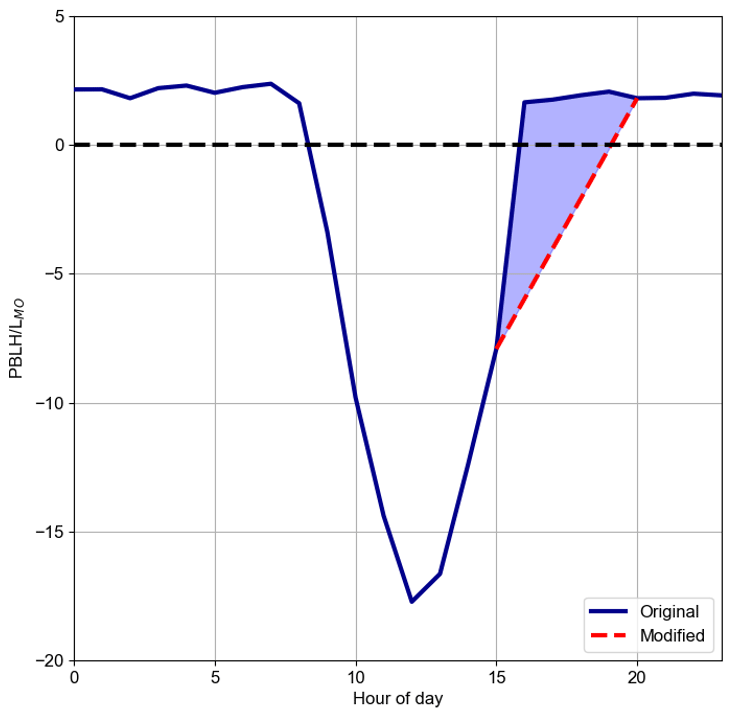
Figure 2Diurnal mean PBLH/L_MO values for the campaign period (blue line). Modified PBLH/L_MO, from 16:00 to 19:00, to account for evening UHI, shown by red dashed line.

Download

During the day, the surface net radiation is partitioned between upwards fluxes of sensible and latent heat and the downwards flux of heat into the ground (Oke, 1982). The version of ADMS-Urban used here (v 4.2) assumes that this ground heat flux is a constant proportion of the net radiation. In reality, this proportion varies diurnally, peaking around midday when a greater proportion of incoming solar radiation is stored by the urban fabric (Anandakumar, 1999; Grimmond and Oke, 1999). The release of this excess heat in the early evening sustains convection in the PBL, prolonging its instability. To account for this, a constant rate of decrease in PBLH/L_MO has been assumed between original modelled values for 15:00 and 20:00, producing the modified campaign period mean PBLH/L_MO diurnal profile illustrated in Fig. 2. Modified L_MO values from 16:00 to 19:00 are added to the set of input meteorological variables for all subsequent simulations, with the directly input PBLH measurements remaining unchanged. This adjustment increases sensible and latent heat fluxes, therefore enhancing the turbulent mixing of air during this early evening period. The 16:00–19:00 time window is chosen as it coincides with sunset in November–December in Beijing, and it is in agreement with the extended duration of evening sensible heat flux decay in urban areas, compared with surrounding rural areas, observed by other UHI-related studies (Zhou et al., 2013; Barlow et al., 2015). Without this adjustment, the model tends to predict overly stable meteorological conditions in the early evening, which can lead to the over-prediction of pollutant concentrations. It is important to note that the modelled surface heat flux and L_MO terms are calculated independently of the PBLH, so that small positive L_MO values can generate an overly stable boundary layer even when paired with the measured MLH assumed here to represent real-world stability conditions.

2.1.4 Background pollutant concentrations

Background pollutant concentrations represent the regional pollution levels on which the local emissions build. For this study, background levels for NO₂, O₃, PM_2.5, PM₁₀, SO₂ and CO are derived directly from hourly air quality measurement data and are assumed to be uniform across the study domain. Measured concentrations at 12 national air quality monitoring stations, run by the China National Environmental Monitoring Center (CNEMC), the IAP field site and an additional site 60 km south-east of Beijing, situated in the built-up Guangyang district of Langfang in Hebei province, are used to estimate this background concentration field. The locations of these 14 sites are given in Table 1.

Table 1Locations (latitude and longitude) of all monitoring stations, including distinction between urban (within the Sixth Ring Road) and suburban site types. The approximate distance (nearest 10 m) from each monitoring station to the nearest road centre line and the corresponding road type are also provided.

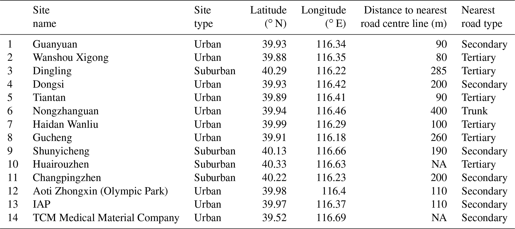
NA – not available

Download Print Version | Download XLSX

For particulate matter (PM_2.5 and PM₁₀), an hourly upwind background concentration is derived based on wind direction with concentrations selected from sites 3 (270–360^∘), 10 (0–90^∘) and 14 (90–270^∘) located to the NW, NE and SE of urban Beijing, respectively. Particulates have near-surface lifetimes of days to weeks; therefore, concentrations in Beijing are heavily influenced by long-range transport (LRT) of both primary and secondary components originating in neighbouring industrial regions (Y. Wang et al., 2017; Cheng et al., 2019). The measured upwind concentration is expected to capture this transported background regional air. Gaseous species such as NO₂ have a much shorter lifetime (∼1 d) and therefore a smaller regional contribution, with concentrations across urban areas dominated primarily by local traffic sources (Zhang et al., 2014). The NO₂ concentrations at the upwind monitoring station were subsequently not deemed representative of the true background value owing to both this greater spatial variation and the proximity of the upwind monitoring stations to local emission sources. Instead, to approximate background values for gaseous species (NO₂, O₃, CO and SO₂), the hourly minimum concentration for each pollutant across the 12 network monitoring stations and the IAP field site is selected, yielding an approximation for the underlying conditions uninfluenced by local sources.

2.2 Emissions inventory processing

For this study, ADMS-Urban simulations use both aggregate 3-D grid source and explicit road source emissions of NO_x, NO₂, SO₂, VOC (total), PM_2.5, PM₁₀ and CO derived from a standard and an optimised version of the high-resolution (3 km) MEIC v1.3 emissions inventory. The standard MEIC v1.3 emissions inventory, for 2013, consists of five emission source sectors: transportation, power, industrial, residential and agricultural (Qi et al., 2017). Note that the latter is not used in this study due to both the lack of farmland in urban Beijing and the negligible contributions to the pollutant species simulated in this study from agricultural emission sources (Qi et al., 2017). The transportation sector is estimated following Zheng et al. (2014), in which county-level emissions, derived from county-level vehicle ownership, are downscaled to grids based on road network and road-specific vehicle activity data. Liu et al. (2015) describe the unit-based technique, adopted to generate the power sector emissions, which utilises the Coal-fired Power Plant Emissions Database (CPED), including information on the technologies, activity data, operation situation, emission factors and locations of individual units. Industrial and residential sector emissions are calculated from provincial-level activity data and emission factors (Zheng et al., 2017). Industrial emissions are downscaled to the county level using GDP (National Bureau of Statistics, 2014), with both industry and residential emissions further distributed to grid-level resolutions based on high-resolution (∼1 km) population density data (Oak Ridge National Laboratory, 2013) (Zheng et al., 2017). To model conditions during the APHH-China winter campaign, the MEIC v1.3 emissions inventory is re-scaled for this study to account for the 2013–2016 emission reductions in Beijing (Sect. 1). According to Cheng et al. (2019), total emissions of NO_x (and NO₂), SO₂, VOCs and PM (PM_2.5 and PM₁₀) in Beijing were estimated to decrease by 30 %, 63 %, 27 %, 35 % and 30 %, respectively, between 2013 and 2016. This adjusted MEIC v1.3 emissions inventory is hereafter referred to as MEIC Std.

An alternate optimised version of MEIC v1.3 (hereafter referred to as MEIC Opt) was created (Li et al., 2018), for November and December 2016, with the aim of addressing the over-allocation of emissions to urban areas that occurs when downscaling MEIC v1.3 to fine scales based on proxy data (Zheng et al., 2017). This MEIC Opt inventory was created using the Nested Air Quality Prediction Modeling System (NAQPMS) to perform iterative minimisation of a cost function comparing NAQPMS simulations with winter campaign observations (Li et al., 2018). This optimisation algorithm was used to redistribute MEIC emissions from central urban Beijing to suburban and rural areas and to adjust their magnitude to represent the campaign period. Both the MEIC Std and MEIC Opt inventories comprise monthly varying emissions with distinct diurnal weighting profiles applied to each emission sector.

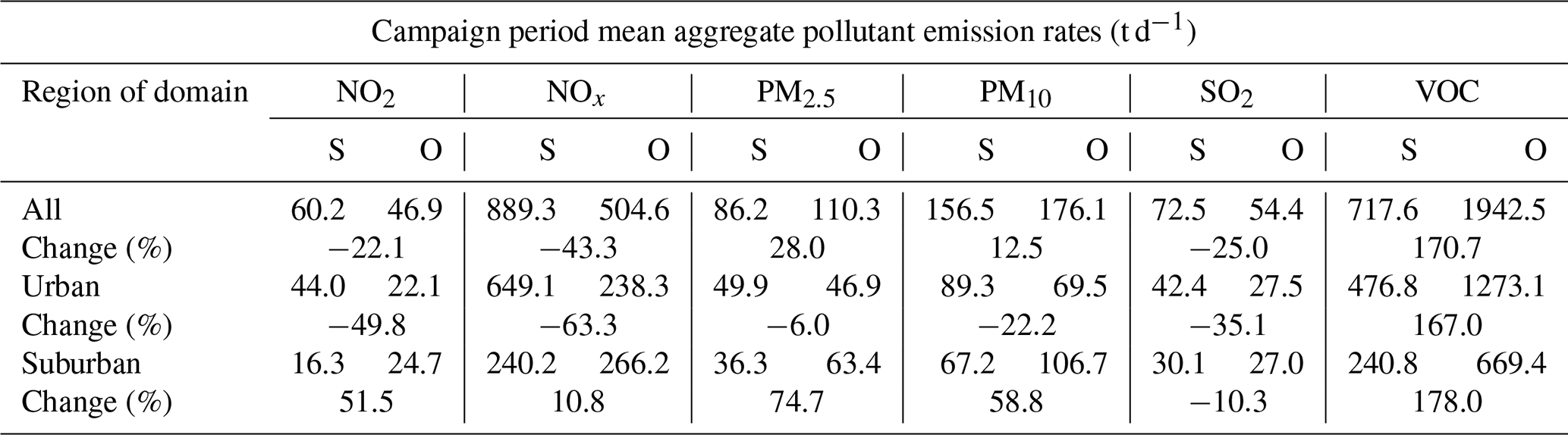
Aggregate 3-D grid sources contain the sum of all MEIC emission source sectors (residential, transportation, industrial and power) and consist of seven vertical layers (38, 90, 152, 228, 337, 480 and 660 m). In the absence of sufficient information required to model point source emissions (e.g. large power plants) explicitly, ADMS-Urban's 3-D grid sources enable plume release and dispersion from each of the seven grid source heights, accounting for tall emission sources included within the MEIC v1.3 power or industrial sector grids. MEIC Std and MEIC Opt campaign period mean NO₂, NO_x, PM_2.5, PM₁₀, SO₂ and VOC emission rates from 3-D grid sources, aggregated across all, urban and suburban grid cells, are shown in Table 2.

Table 2Campaign period mean MEIC Std (S) and MEIC Opt (O) pollutant species emissions (t d⁻¹) aggregated across all, urban and suburban grid cells. Change (%) in emissions between inventories, following optimisation, calculated as (O – S/S) ×100.

Download Print Version | Download XLSX

An explicit network of road emissions for Beijing has been constructed based on the MEIC transportation sector emissions. Figure 3 illustrates the pseudo top–down approach adopted here in the absence of detailed information on traffic activity and fleet composition. Figure 3a shows the spatial distribution of the November and December mean MEIC Std transportation sector surface NO₂ emissions. The transportation sector emissions of all pollutants are apportioned to individual road segments on a grid cell-by-grid cell basis, using the ArcGIS geographic information system software. The spatial road network of Beijing, presented in Fig. 3b, is provided by the OpenStreetMap dataset (https://openstreetmap.org/, last access: 6 June 2019) and includes individual road segment type and geometry information. Emissions are mapped onto the road network based on each road segment length and an emissions weighting factor, producing the distribution shown in Fig. 3c, following Eq. (1):

where l_i,j represents the length of road segment i in grid cell j of road type k. The weighting factor of road type k is given by w_k. E_j and n denote the total traffic emissions and number of road segments in grid cell j, respectively. A weighted mean emission rate, based on road segment length, is calculated along segments traversing multiple grid cells in order to avoid discontinuities.

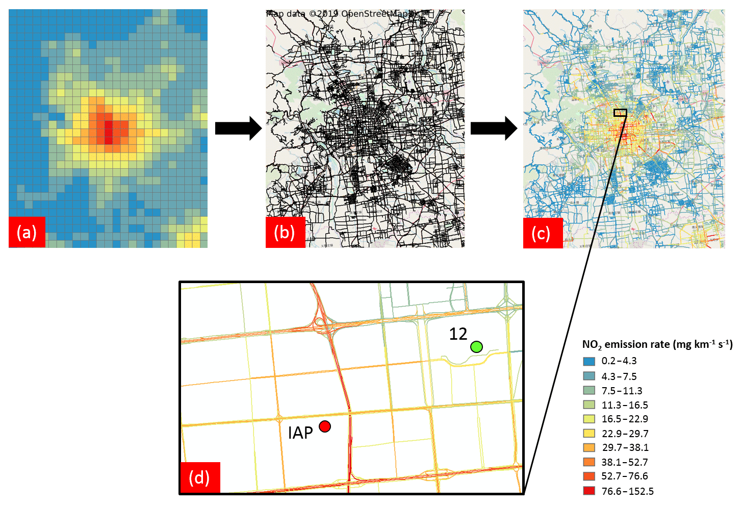
Figure 3(a) Spatial distribution of November and December mean transportation sector MEIC Std NO₂ emissions (lowest vertical layer) covering the full study domain, (b) spatial road network of Beijing (source: OpenStreetMap, © OpenStreetMap contributors 2019. Distributed under a Creative Commons BY-SA License), (c) explicit road source NO₂ emission rates following apportioning of (a) onto (b), and (d) enlarged section of the road emissions network covering the IAP field site and site 12.

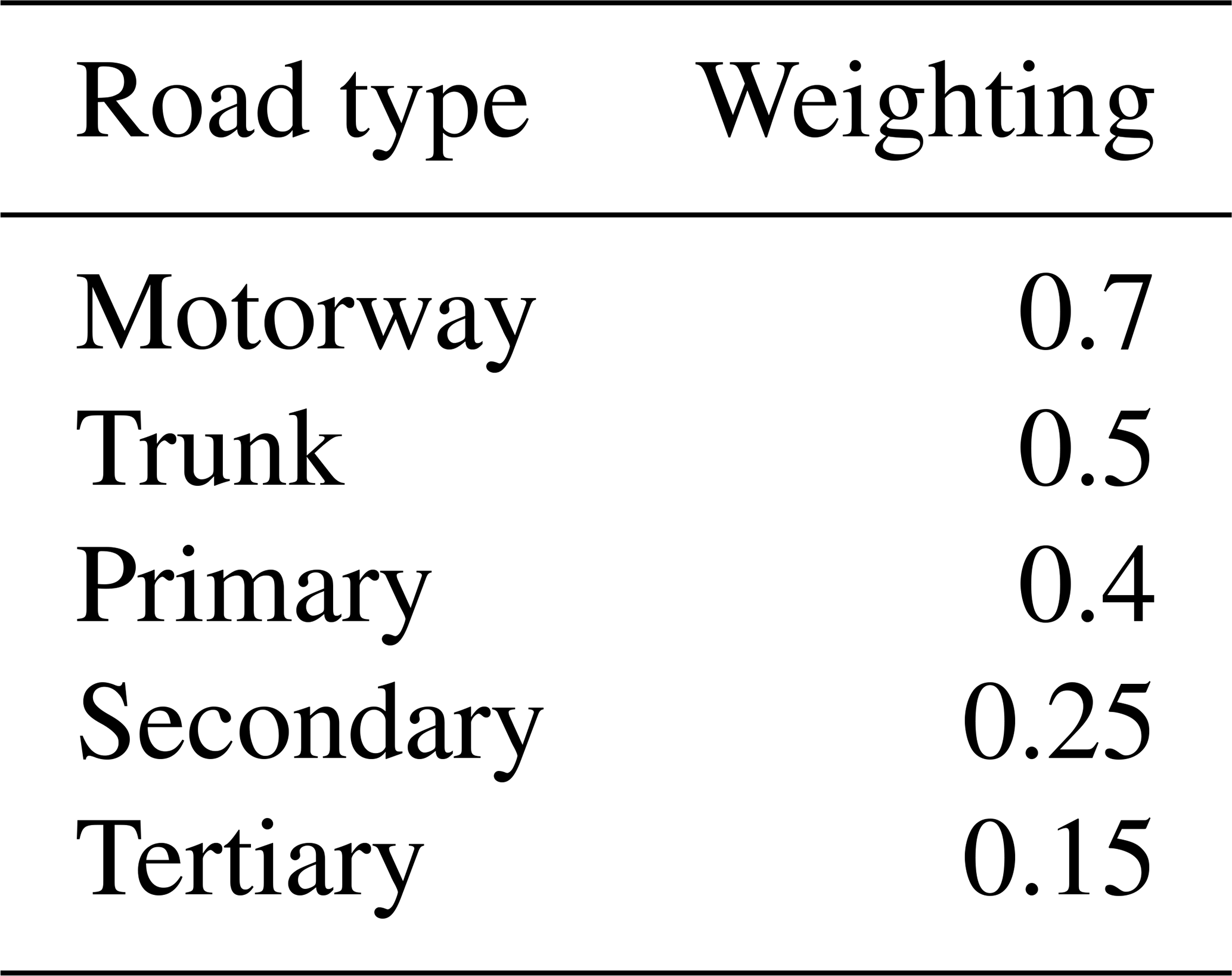
Weighting factors (Table 3) are estimated using road type and width (based on manual inspection of the most frequent number of lanes for each road type), acting as proxies for traffic activity. Each road type weighting factor is applied equally to all pollutant species. The magnitude of weighting factors relative to each other is important, rather than their absolute values, according to Eq. (1). Minor roads were removed from the network to limit the computational expense of each simulation and are instead aggregated within the 3-D grid sources. This methodology is based on the assumption that traffic volume, speed and fleet composition are constant across all road type classes listed in Table 3. However, substantial variations in traffic flow characteristics on roads of the same classification within Beijing's urban area have been observed. For example, Jing et al. (2016) used GPS-fitted buses and taxis to collect near real-time traffic data along the major road types in Beijing, finding much greater levels of congestion closer to the urban centre, causing increased traffic volume and vehicle speed variations. Additionally, Y. Zhang et al. (2018) observed a greater proportion of vehicles with lower emission standards on roads outside the Fifth Ring Road. Given that the same emission weighting factors for roads of the same class are applied across the domain and the lack of traffic flow variations on specific roads within cities in the MEIC framework (Zheng et al., 2014), the methodology adopted here may under-allocate emissions on more congested inner-city roads and over-allocate emissions in suburban areas.

Table 3Estimated emission weighting factors for each modelled road type.

Download Print Version | Download XLSX

2.3 Model evaluation

Evaluation of regional-scale Eulerian CTMs involves the comparison of measurements at specific monitoring site locations with simulated concentrations in the nearest model grid box (Zhong et al., 2016; Y. Wang et al., 2017; Zheng et al., 2017). However, for street-scale air quality modelling with ADMS-Urban, pollutant concentrations can be simulated at specific locations, referred to hereafter as receptor points. For this study, concentrations are modelled at the locations of the 12 monitoring network stations, as well as the IAP field site, for direct comparison with the corresponding measured concentrations. The following three statistical performance measures are considered simultaneously, enabling a comprehensive evaluation of modelled predictions of concentrations, using both MEIC Std and MEIC Opt emissions inventories, during the APHH-China winter campaign period.

where n denotes the total number of matching hourly modelled and observed concentrations; $\stackrel{\mathrm{‾}}{M}$ and $\stackrel{\mathrm{‾}}{O}$ indicate mean modelled and observed concentrations, respectively, and σ is the standard deviation.

NMSE (ideal value =0) is a measure of the model's overall accuracy (Cai and Xie, 2011), incorporating the effects of both systematic and random errors (Patryl and Galeriu, 2011); Fb (ideal value =0) reflects the model's tendency to overestimate or underestimate concentrations, compared to measurements; and R (ideal value =1) informs on the extent to which modelled and measured values are linearly related.

In this study, the statistical evaluation of pollutant concentrations simulated at the exact coordinates of the measurement locations is complemented by street-scale-resolution maps which more clearly illustrate the strong spatial heterogeneity of pollution levels across Beijing. Fully resolved PM_2.5, NO₂ and O₃ concentration fields in central Beijing are simulated with a combination of regularly spaced receptor points at ∼150 m and additional output points distributed within and in the immediate vicinity of all individual road emission source segments. The addition of emission source-oriented output points increases the model resolution to <10 m across regions containing dense distributions of explicit road sources, therefore enabling the sharp pollutant concentration variations adjacent to roads to be captured.

3.1 Street-scale variation of PM_2.5, NO₂ and O₃ concentrations

Mean PM_2.5, NO₂ and O₃ concentrations simulated for the campaign period (5 November–10 December 2016), using the MEIC Opt inventory, for a region of urban Beijing within the Fifth Ring Road are presented in Fig. 4. The influence of the explicit road emissions network on the spatial variation of all species is clear, most notably along the Second, Third and Fourth Ring Roads. PM_2.5 and NO₂ concentrations peak at 125 and 160 µg m⁻³, respectively, along the ring road centre lines, before sharply decaying. The magnitudes of this drop and distance across which it occurs are determined not only by emission source strength, but also by physical and chemical mechanisms, with the speed of plume dispersion and mixing, controlled by mechanical and convective turbulence generation, interacting with the differing lifetimes of individual pollutants. In Fig. 5, mean NO₂ concentrations decrease by ∼20–25 µg m⁻³ along a horizontal profile extending 100 m either side of the Second Ring Road. The spatial variation of O₃ concentrations is approximately inversely related to these NO₂ levels. Modelled O₃ concentrations decrease to 5 µg m⁻³ along the Second Ring Road centre line and reach 25 µg m⁻³ between the Fourth and Fifth Ring Roads (Fig. 4). This is a result of the fast reaction of O₃ with NO (titration) (Reaction R4) which dominates in high-NO_x environments (Y. Zhang et al., 2015; Tang et al., 2017; Ma et al., 2018), such as those next to major roads. The conversion of primary NO exhaust emissions to NO₂, following the titration of O₃, also produces a sharply increasing NO₂∕NO_x ratio with distance from the road centre (Fig. 5). In the following sections, a comprehensive evaluation of the model performance is presented.

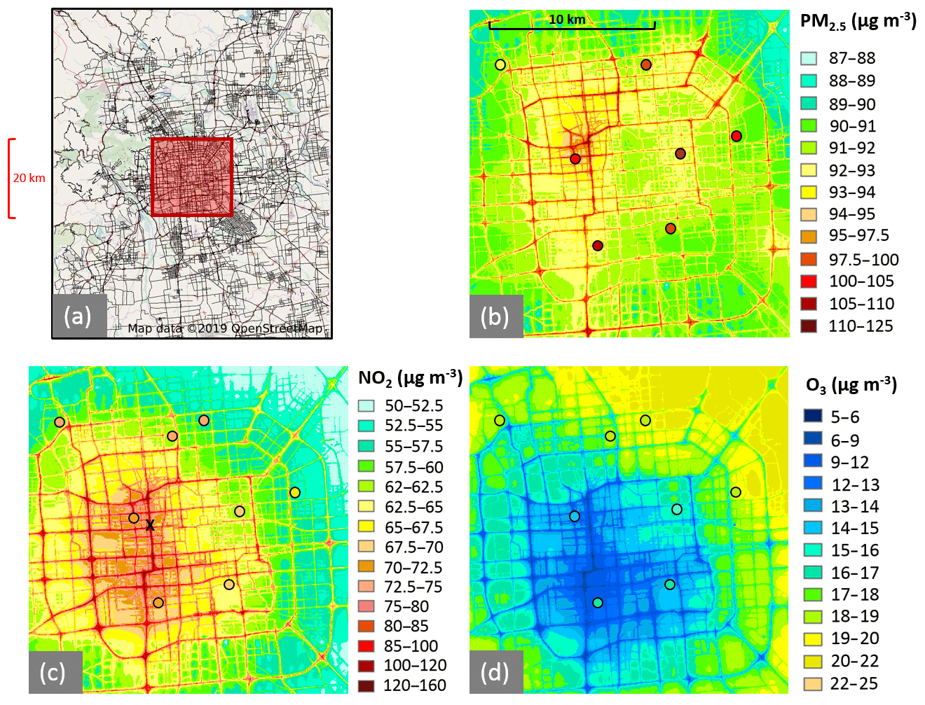
Figure 4Spatial maps of mean PM_2.5 (b), NO₂ (c), and O₃ (d) concentrations for the winter campaign period (5 November to 10 December 2016), simulated using the MEIC Opt emissions inventory. Simulated concentrations cover the region marked in (a). Mean measured concentrations at monitoring network sites (NO₂, O₃ and PM_2.5) and the IAP field site (NO₂ and O₃) are represented by coloured dots. © OpenStreetMap contributors 2019. Distributed under a Creative Commons BY-SA License.

Figure 5Simulated campaign period mean NO₂ concentrations, with distance from the point on the Second Ring Road centre line (marked by X in Fig. 4c) using MEIC Opt (pink). Simulated NO₂∕NO_x ratio denoted by a black dashed line. Shaded areas represent the 95 % confidence interval.

Download

3.2 Model evaluation and assessment of emission inventories

Table 4 summarises the performance of ADMS-Urban in Beijing during the APHH-China winter measurement campaign, with comparisons between MEIC Std and MEIC Opt simulations enabling an assessment of the MEIC v1.3 optimisation.

Table 4Statistical evaluation of modelled pollutant concentrations for the campaign period, using MEIC Std (S) and MEIC Opt (O) emissions inventories. Mean modelled (Mod) and observed (Obs) concentrations and statistics divided into all (12 monitoring network sites and the IAP field site for NO₂ and O₃, monitoring network sites only for PM_2.5) and urban and suburban monitoring site groups. Urban and suburban sites defined in Table 1. NO_x measurements only available at the IAP field site. Mean concentrations and statistics calculated from matching hourly values.

Download Print Version | Download XLSX

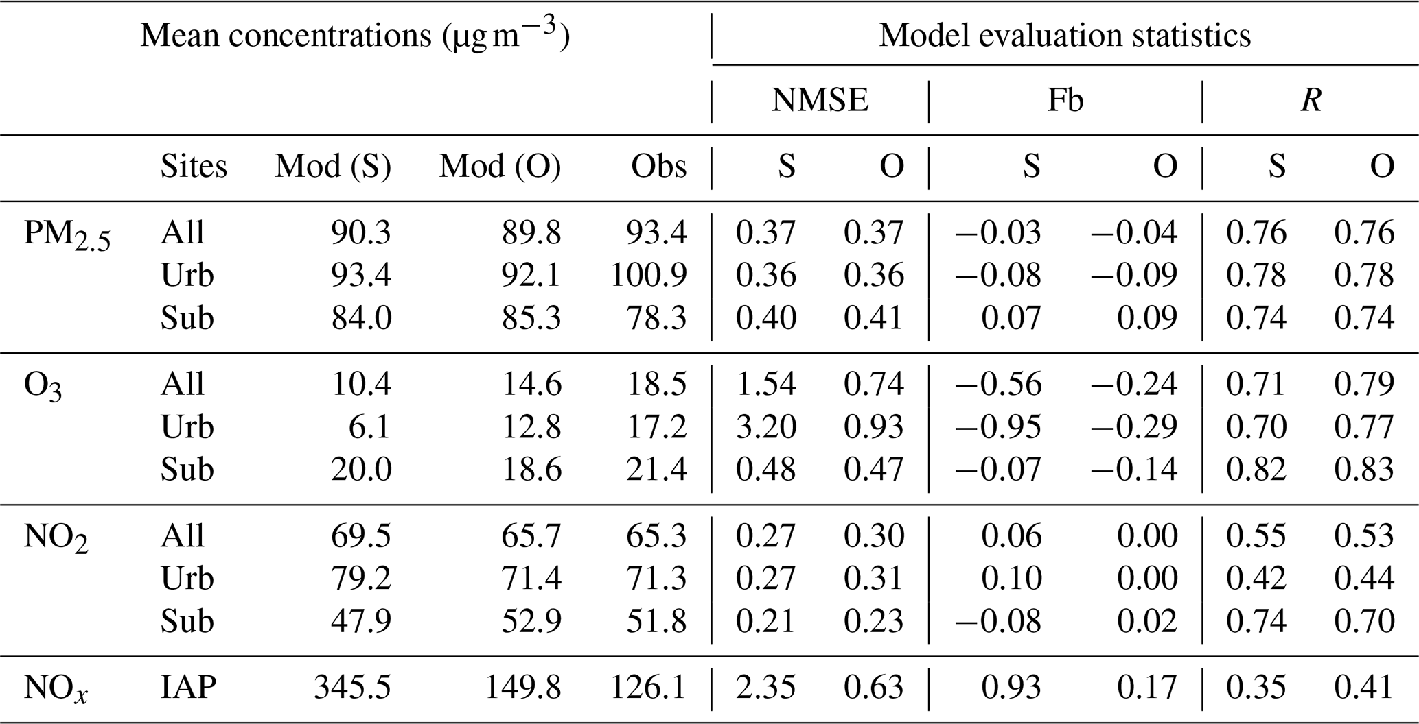
Modelled NO_x concentrations at the IAP field site display the most substantial differences between the two simulations (Table 4; Fig. 6). Modelled NO_x concentrations using the MEIC Opt inventory are 149.8 µg m⁻³, 56 % lower than the MEIC Std case, leading to NMSE and Fb decreases from 2.35 to 0.63 and 0.93 to 0.17, respectively (Table 4). This enhanced model agreement is reflected in Fig. 6, in which a large proportion of modelled NO_x values reaching 400–600 µg m⁻³ with MEIC Std, up to a factor of 6 higher than measurements, is reduced to within a factor of 2 of measured concentrations using MEIC Opt. This result reflects the 63 % NO_x emissions reduction across urban Beijing, over all source sectors, in the optimised inventory (Table 2). However, correlation coefficient (R) values for simulated NO_x remain low using both emissions inventories, slightly increasing from 0.35 to 0.41 with MEIC Opt. This smaller improvement in the correlation between measured and modelled NO_x using MEIC Opt, compared to NMSE and Fb, reflects the dependency of R on modelled NO_x levels that capture the correct temporal variation as well as the overall magnitude of NO_x measurements. The noise apparent in the measured and simulated NO_x comparison in Fig. 6 is therefore likely related to either the diurnal emissions profile or meteorological variations.

Figure 6Hourly measured and modelled NO_x concentrations during the campaign period at the IAP field site. Panels (a) and (b) show concentrations simulated using MEIC Std and MEIC Opt, respectively. Colours represent the total number of matching hourly measured and modelled values contained within distinct hexagonal bins. Dashed lines mark a factor of 2 difference between measured and simulated concentrations.

Download

NO₂ concentrations differ less, with NMSE values of 0.27 and 0.30 for the MEIC Std and MEIC Opt simulations, respectively. However, a greater difference is evident at urban receptor locations, with modelled NO₂ concentrations from the MEIC Opt simulation 12 % lower than those with MEIC Std. Across suburban sites, the opposite pattern is seen, with changes in Fb values between measurements and MEIC Std and MEIC Opt simulations ranging from negative (−0.08) to positive (0.02), respectively. Both urban and suburban NO₂ concentration changes, between simulations, reflect the overall redistribution of NO₂ emissions in the MEIC Opt inventory, away from central Beijing and towards the city outskirts (Table 2).

The much greater urban NO_x concentration difference between the two simulations, as compared to NO₂, can be attributed to two factors. Firstly, NO₂ concentrations respond in a more non-linear way to NO_x emission changes than NO_x concentrations. This has been shown in previous studies (e.g. Kurtenbach et al., 2012) and can be explained by the timescales and kinetics involved in the formation and destruction of secondary NO₂. As NO_x levels decrease, the production of secondary NO₂ via Reaction (R4) occurs faster as O₃ concentrations are higher, leading to a slower rate of decrease of NO₂ concentrations compared to NO_x emissions. Additionally, the proportion of NO_x directly emitted as NO₂ is greater with MEIC Opt (${\mathrm{NO}}_{\mathrm{2}}/{\mathrm{NO}}_x=\mathrm{0.093}$) than MEIC Std (${\mathrm{NO}}_{\mathrm{2}}/{\mathrm{NO}}_x=\mathrm{0.068}$) (Table 2). This is reflected by the much greater reduction, from MEIC Std to MEIC Opt, in domain-aggregated NO_x emissions (43 %), as compared NO₂ (22 %) (Table 2).

At urban sites, O₃ concentrations simulated with MEIC Opt are 12.8 µg m⁻³, which is a factor of 2 greater than those simulated using MEIC Std (6.1 µg m⁻³). Overall, the modelled O₃ concentrations at urban sites using MEIC Opt are in closer agreement with the measurements, reflected by lower Fb and NMSE values of −0.29 and 0.93, respectively, as compared to −0.95 and 3.2 in the MEIC Std simulations (Table 4). This is caused by both lower urban NO_x emissions in MEIC Opt and the reduced proportion of remaining NO_x emitted directly as NO, in MEIC Opt, leading to less O₃ destruction through Reaction (R4). Contrastingly, higher MEIC Opt NO_x emissions in suburban Beijing reduce modelled O₃ concentrations by 7 %. As a result, modelled O₃ performance across all monitoring stations is substantially improved in the MEIC Opt simulation, with a NMSE reduction from 1.54 to 0.74 and an R value increase from 0.71 to 0.79 (Table 4). These results highlight the strong dependency of O₃ concentration predictions in urban areas, which inform human exposure analyses and influence future emission control implementation, on the accurate spatial variation and magnitude of NO_x emissions in high-resolution emissions inventories. The increase in modelled urban O₃ concentrations following NO_x emissions reductions also highlights both the negative impact that controls on one pollutant species can have on another as well as the possible need for air quality guidelines that consider multiple pollutants, in contrast to the single pollutant-based air quality index used in China (Han et al., 2018).

Figure 7a and b illustrate site-specific differences between measured and simulated NO₂ and O₃ concentrations, respectively, using both emissions inventories. It is clear that, despite generally closer model agreement with measurements using MEIC Opt, NO₂ concentrations remain substantially overestimated at urban sites 1 (∼14 µg m⁻³) and 2 (∼9 µg m⁻³). To help understand the cause of this, the sensitivity of modelled concentrations within 100 m of a road source near site 1 is illustrated in Fig. 8. Concentrations along a cross-road slice, extending 100 m either side of the road, are simulated after halving and doubling the magnitude of emissions of all species from this secondary road. Emissions from all other sources in the model configuration remain the same. Along the road centre, the range of simulated concentrations between emission scenarios is ∼10 µg m⁻³; however, this difference decreases to ∼2 µg m⁻³ at a distance of 100 m, which is much lower than modelled NO₂ overestimations produced by MEIC Opt at sites 1 and 2, each located ∼80–90 m from the nearest road. Therefore, the high modelled NO₂ at sites 1 and 2 may only be partially attributed to an over-allocation of explicit road source emissions caused by either (a) underlying gridded emissions that are still too high or (b) not considering traffic volume/speed variations across the domain in road class emission weighting factor estimates. It should also be noted that the physical barriers to pollution dispersion represented by the urban canopy, and specifically street canyons, are not explicitly modelled in this study. This may lead to road emissions dispersing further from the road centre than in reality, therefore contributing to elevated modelled concentrations at greater distances from explicit road sources (Dédelé and Miskinyte, 2015). The sensitivity of the simulated NO₂∕NO_x concentration ratio to emission magnitude changes is also shown in Fig. 8. For each emissions scenario, the NO₂∕NO_x emissions ratio remains the same (0.093) (Table 2); however, the concentration ratio varies. With doubled NO_x emissions, the NO₂∕NO_x ratio is ∼0.3 along the road centre, compared to ∼0.4 with halved NO_x emissions (Fig. 8). This difference, which decays to zero at a distance of ∼75 m, is mostly driven by PBL dynamics and the mixing of freshly emitted NO_x into air with a lower NO₂∕NO_x concentration ratio driven by the impact of higher NO_x emissions on secondary NO₂ production via Reaction (R4), as discussed above.

Figure 7Campaign period mean measured and modelled (a) NO₂, (b) O₃, and (c) PM_2.5 concentrations at all monitoring network sites (numbered) and the IAP field site (NO₂ and O₃). Blue and pink lines indicate concentrations simulated using MEIC Std and MEIC Opt, respectively. Horizontal light blue line represents campaign period mean background concentrations calculated from measurements.

Download

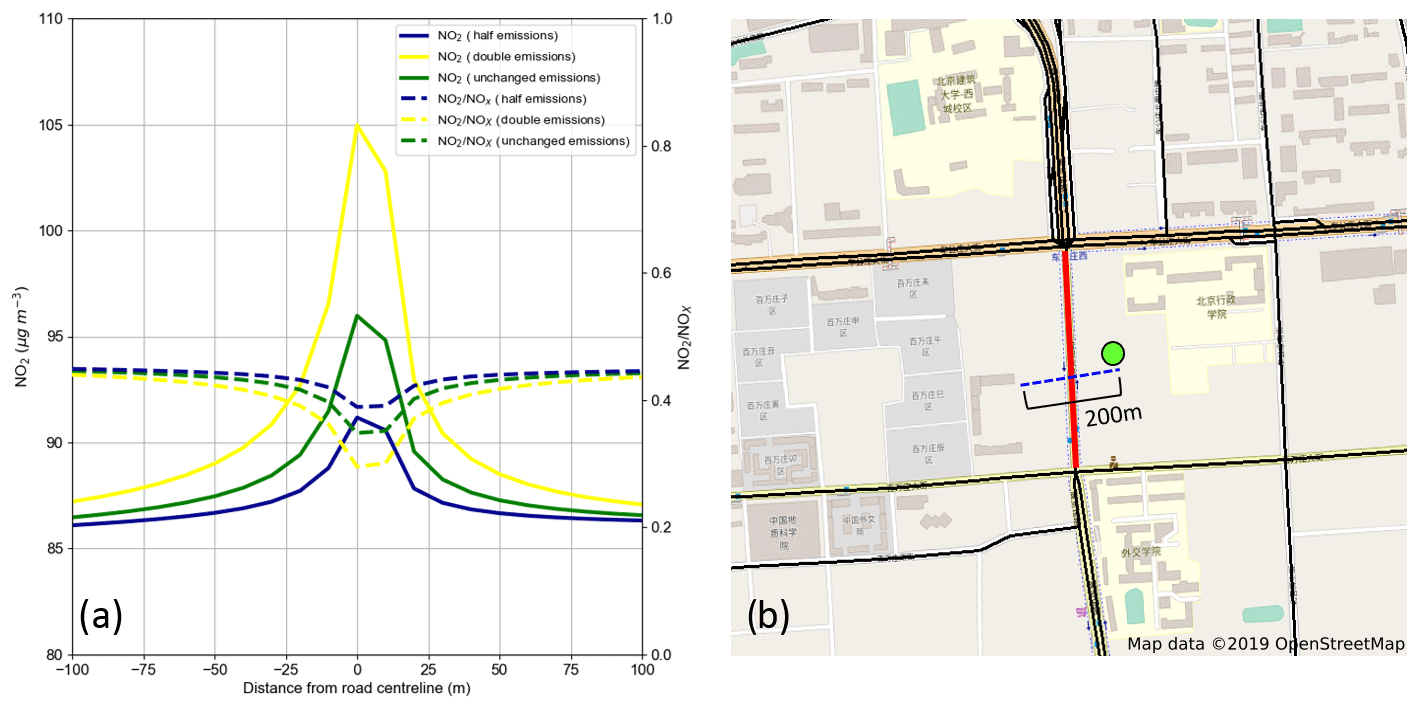
Figure 8(a) Campaign period mean simulated NO₂ concentrations and NO₂∕NO_x concentration ratios with distance from the road centre along the cross-road slice marked in (b) using half (blue), double (yellow) and unchanged (green) emissions of all species from an explicit road source marked by red line. The green circle in (b) marks the position of monitoring site 1. (b) © OpenStreetMap contributors 2019. Distributed under a Creative Commons BY-SA License.

A clear distinction exists between measured PM_2.5 concentrations recorded at the suburban (78 µg m⁻³) and urban (101 µg m⁻³) monitoring stations (Table 4). These values are well in excess of China's annual PM_2.5 National Ambient Air Quality Standard (NAAQS) of 35 µg m⁻³; however, concentrations are expected to be higher in winter due to more stable meteorology (Zheng et al., 2015; Li et al., 2017) and enhanced coal combustion for residential heating and cooking and at power plants in neighbouring cities (Chen et al., 2017). Simulated PM_2.5 concentrations, however, do not reflect such an urban–suburban discrepancy, with mean urban values exceeding those at suburban sites by only 9 and 7 µg m⁻³ using MEIC Std and MEIC Opt, respectively (Table 4). Across all monitoring stations, the range in campaign period mean measured concentrations is substantially higher (∼40 µg m⁻³) than the simulated range using both MEIC Std (∼20 µg m⁻³) and MEIC Opt (∼15 µg m⁻³), respectively. These results suggest that either PM_2.5 emission sources are too uniform in magnitude and spatial distribution across the domain in the current model set-up or that the assumption of a homogeneous background PM_2.5 concentration is invalid. It is likely that, by diluting PM_2.5 emissions within individual grid cells and not explicitly representing point source emissions (e.g. large industrial units), the model is unable to capture the PM_2.5 concentration hotspots that would increase the urban PM_2.5-level increment and improve model agreement with the observed spatial variation. With the exception of simulated PM_2.5 adjacent to major roads, this modelled uniformity in urban PM_2.5 is clearly evident in Fig. 4, in which PM_2.5 concentrations vary by only ∼5–10 µg m⁻³ across the area enclosed by the Fifth Ring Road. The mean estimated PM_2.5 background concentration is 79 µg m⁻³ (Fig. 7), which is higher than both the mean measured concentrations at suburban sites 3 and 10, located to the north. This implies that either the background PM_2.5 level is, in reality, inhomogeneous with lower concentrations to the north and higher to the south of urban Beijing or that the upwind background monitoring site to the south is too heavily influenced by local emission sources and is not representative of background conditions. The relative contributions from PM_2.5 emission sources and background inhomogeneity to the underestimated spatial variation in PM_2.5 is further discussed in Sect. 3.4.

3.3 Winter campaign diurnal cycles of NO₂, O₃ and NO_x

The diurnal variation of pollutant species in urban areas provides insight into how concentrations are impacted by both diurnal variations in meteorology and temporally varying emissions. The locations of urban stations 1, 12 and IAP, and suburban site 11 are illustrated in Fig. 9, with measured mean diurnal NO₂ concentrations averaged over the campaign period at all four sites compared with those simulated using both the MEIC Std and MEIC Opt inventories in Fig. 10. There are several common differences between modelled and measured concentration profiles at all three urban stations (Fig. 10a, c and d). Firstly, both simulated NO₂ diurnal cycles at sites 1, 12 and IAP are considerably lower than measurements from 23:00 to 06:00. This discrepancy peaks at 02:00, with simulated concentrations ∼20 and ∼30 µg m⁻³ lower than measurements, using MEIC Std and MEIC Opt, respectively. Observed NO₂ concentrations at urban sites remain elevated between 23:00 and 06:00, relative to the rest of the day, resulting in a diurnal profile absent of the distinct morning and evening peaks commonly observed in other megacities, such as London (Hood et al., 2018). High nocturnal NO₂ concentration measurements during the APHH-China winter campaign at the IAP field site are also noted by Shi et al. (2019).

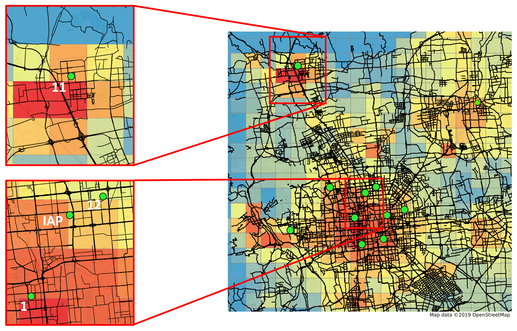
Figure 9Spatial distribution of November and December mean MEIC Opt NO₂ emissions (all emission sectors) overlaid with Beijing road network (source: OpenStreetMap, 2019). Enlarged regions cover urban sites 1, 12 and IAP as well as suburban site 11. Right panel: © OpenStreetMap contributors 2019. Distributed under a Creative Commons BY-SA License.

Figure 10Campaign period mean diurnal variation in modelled and measured NO₂ concentrations at sites (a) 1, (b) 11, (c) 12, and (d) IAP. Modelled concentrations produced using both MEIC Std (blue) and MEIC Opt (pink). Measurements marked by red line. Shaded areas and error bars represent the 95 % confidence intervals for simulated and measured concentrations, respectively.

Download

Previous studies have attributed the evening influx of heavy duty diesel trucks (HDDTs), banned from commuting within the Fourth Ring Road from 06:00 to 23:00 (Zhang et al., 2019), to evening NO_x concentration increases across urban Beijing of up to 10 µg m⁻³ (Wu et al., 2016; Yang et al., 2019). A large proportion of this HDDT fleet originates in other provinces where emission standards are not as strict as those in Beijing (Wang et al., 2011). It is possible, therefore, that in a proxy-based emissions inventory (e.g. MEIC), such traffic restrictions and inter-provincial vehicle mobility are not fully accounted for (Zheng et al., 2014). This is supported by the much closer agreement between evening modelled and measured NO₂ at suburban site 11 (Fig. 10b), situated outside the Sixth Ring Road (Fig. 9) and away from the influence of additional nighttime HDDT NO_x emissions. Additionally, ADMS-Urban makes an approximation when modelling dispersion in calm conditions by applying a minimum wind speed of 0.75 m s⁻¹ (CERC, 2017). These stable, low wind speed conditions, however, are common in winter in Beijing and have been strongly linked to the acceleration of pollution accumulation during severe winter haze events (X. Zhang et al., 2015; Z. Zhang et al., 2016; L. Zhang et al., 2018). Therefore, it is likely that the large early morning NO₂ concentration model underestimations across all three urban sites are a consequence of NO_x emissions that are too low in magnitude, from 23:00 to 06:00, dispersing into a simulated PBL that may be insufficiently stable due to the use of a minimum wind speed in the model.

From 06:00 to 09:00, modelled NO₂ concentrations in both the MEIC Std and MEIC Opt simulations increase sharply (Fig. 10). This is most prominent at site 1, where simulated levels approximately double during this 3 h period. This increase corresponds to the release of rush hour traffic-related NO_x emissions into a stable and shallow morning PBL. Contrastingly, measurements at these sites decline over this early morning period following an evening concentration peak as described above. This overestimation of NO₂ continues throughout the afternoon, with similar profiles at sites 12 and IAP reflecting the close proximity of both receptor locations (∼3 km apart) (Fig. 9).

The concurrence of evening rush hour traffic emissions and a stabilising PBL, associated with the reduction in surface heating following sunset, creates a second simulated NO₂ concentration peak at ∼18:00. In contrast to the simulated morning concentration rise, the close agreement between the measured and modelled times of onset and magnitude of this early evening increment indicates that the simulated stability adjustment (Sect. 2.1.2), implemented between 16:00 and 19:00, has successfully accounted for the re-release of stored heat, characteristic of large urban areas.

There is little difference between the diurnal NO₂ concentration profiles simulated using the MEIC Std and MEIC Opt inventories, and this is consistent with the model evaluation results described in Sect. 3.2. Simulated NO₂ concentrations across the urban sites are marginally lower using MEIC Opt compared to MEIC Std, with the reverse true at suburban site 11, again reflecting the relocation of emissions out of the urban centre.

The much closer agreement between measured NO_x concentrations at the IAP field site and those simulated with MEIC Opt compared to MEIC Std, outlined in Sect. 3.2, is further emphasised by the diurnal cycles in Fig. 11. MEIC Opt produces much lower NO_x concentrations than MEIC Std across all hours of the day (up to a factor of 3), peaking during morning and evening rush hour with concentrations of ∼200 and ∼250 µg m⁻³, respectively. The simulated NO₂∕NO_x concentration ratio at IAP produced with MEIC Opt ranges from 0.4 to 0.7 throughout the day, 0.2–0.3 greater than the MEIC Std simulation. This again reflects the combined influences of both the greater NO₂∕NO_x emission ratio in MEIC Opt (Table 2) and the non-linear response of secondary NO₂ concentrations to NO_x emission changes, as discussed in Sect. 3.2. Overestimated NO_x concentrations and underestimated NO₂∕NO_x concentrations ratios at IAP produced with MEIC Opt indicate that, despite emissions modifications, the magnitudes of NO_x emissions (specifically NO) are too high in the MEIC Opt inventory.

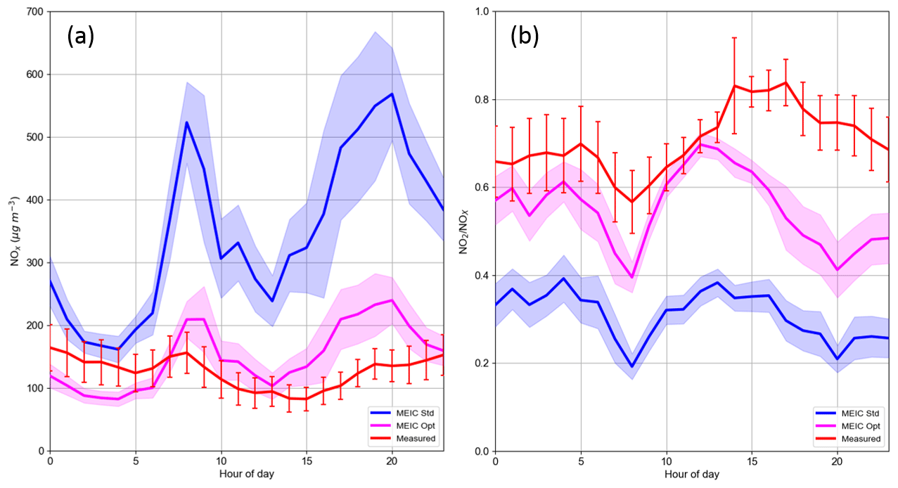
Figure 11Campaign period mean diurnal variation in modelled and measured (a) NO_x concentrations and (b) NO₂∕NO_x concentration ratios at the IAP field site. Modelled concentrations produced using both MEIC Std (blue) and MEIC Opt (pink). Measurements marked by red line. Shaded areas and error bars represent the 95 % confidence intervals for simulated and measured concentrations, respectively.

Download

The impact of NO_x emission differences on diurnal O₃ concentrations is illustrated in Fig. 12. Using MEIC Std, simulated O₃ concentrations across all three urban sites are considerably lower than measured values from 08:00 to 17:00, with the measured–modelled difference reaching ∼20 µg m⁻³ at midday. This reflects the prominence of Reaction (R4), caused by high urban NO emissions in MEIC Std. The reverse response is seen at site 11, where midday O₃ is overestimated by ∼10 µg m⁻³ as a result of low MEIC Std NO emissions in suburban versus urban regions. During daylight hours, there is much closer agreement between measured and modelled O₃ across all four sites with MEIC Opt. This reflects the adjusted balance between photochemical production of O₃, via Reaction (R3), and its removal via Reaction (R4), caused by decreased NO_x emissions in urban areas and increased emissions in suburban areas, in the MEIC Opt inventory. NO_x–O₃ chemistry is also greatly influenced by proximity to road sources. As shown in Fig. 8 and discussed in Sect. 3.2, roads with higher NO_x emissions lead to lower NO₂∕NO_x concentration ratios within distances of 100 m and therefore greater O₃ loss through its titration by NO in Reaction (R4).

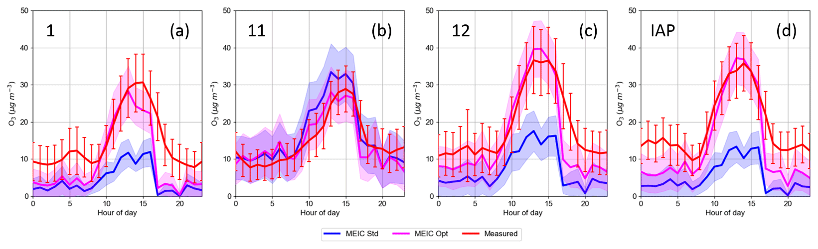
Figure 12Campaign period mean diurnal variation in modelled and measured O₃ concentrations at sites (a) 1, (b) 11, (c) 12 and (d) IAP. Modelled concentrations produced using both MEIC Std (blue) and MEIC Opt (pink). Measurements marked by red line. Shaded areas and error bars represent the 95 % confidence intervals for simulated and measured concentrations, respectively.

Download

3.4 Local and regional contributions to PM_2.5 concentrations

Figure 13 presents the diurnal variation of the range of site-specific campaign period mean measured and simulated PM_2.5 concentrations, using MEIC Opt, across all 12 monitoring network sites. The interquartile range of all network measurements, illustrating the extent to which PM_2.5 concentrations vary spatially across the domain, greatly exceeds that of modelled concentrations for most of the day. This observed range is largest at night and consistently in excess of 20 µg m⁻³, compared to the simulated range of 5–10 µg m⁻³. The measured ranges are additionally sub-divided into those recorded at urban and suburban monitoring sites, with the diurnal median urban PM_2.5 values as much as ∼35 µg m⁻³ higher than those for suburban sites between 23:00 and 02:00. It is possible that, similarly to the elevated evening NO₂ concentration measurements discussed in Sect. 3.3, this high measured nighttime urban PM_2.5 concentration increment is also related to the influx of HDDTs to central Beijing following the lifting of traffic restrictions from 23:00 to 06:00, with recent studies (Y. Zhang et al., 2015; Wu et al., 2016) reporting a rising contribution from HDDT exhaust emissions to PM_2.5 levels across China. A subsequent reduction of the measured urban–suburban PM_2.5-level discrepancy during daytime hours, reaching ∼10 µg m⁻³ at midday, coincides with much closer overall agreement between modelled and measured concentrations.

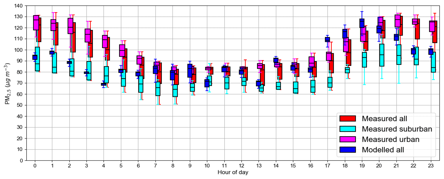
Figure 13Variations in site-specific campaign period mean measured (red) and modelled (blue) PM_2.5 concentrations across all monitoring network stations for each hour of the day. Measurements sub-divided to highlight the variation between suburban (cyan) and urban (pink) monitoring network stations specifically.

Download

The large difference between mean measured urban and suburban PM_2.5 concentrations throughout the day in Fig. 13 is not captured by the model. This is likely the result of either a lack of heterogeneity in the modelled PM_2.5 emission sources, particularly across urban areas, or that, in reality, substantial non-uniformity in the background concentration exists across the domain. The former is consistent with a number of previous studies on PM_2.5 source apportionment in Beijing, which have suggested that, during extended periods of elevated particulate mass concentrations in winter, local emissions can account for 80 % of PM_2.5 concentrations (Li et al., 2017; Y. Wang et al., 2017; Chang et al., 2019). Therefore, as discussed in Sect. 3.2, in order to simulate the high spatial variation of PM_2.5 concentrations, characterised by large urban PM_2.5 concentration increments, higher-resolution modelling of primary PM_2.5 emissions through the inclusion of explicitly represented large point sources is likely to be necessary.

It is also possible that greater secondary aerosol production needs to be included in the model's chemistry scheme, further increasing the simulated urban PM_2.5 increment. Currently in ADMS-Urban, with the exception of ammonium sulfate production, secondary PM_2.5 concentrations are assumed to be included in the upwind background concentration. As the dominant contribution to secondary PM_2.5 in Beijing is reported to be from neighbouring industrial regions to the south (Ma et al., 2017), this assumption seems largely valid. However, the relative local contributions of other secondary components in Beijing, such as ammonium nitrates, are found to be increasing (Y. Wang et al., 2017; Xu et al., 2019; Yang et al., 2019). This is a consequence of the effectiveness of recent SO₂ emission controls and the lack of agricultural ammonia (NH₃) emissions reductions (Zheng et al., 2018), which have promoted the formation of ammonium nitrate (Xu et al., 2019). Xu et al. (2019) also found the nitrate aerosol to be of increasing importance at night during winter, as a result of its greater stability at lower temperatures, which, coupled with high nighttime NO₂ concentrations (Fig. 10), may further account for the elevated evening PM_2.5 levels (Fig. 13). The applicability of this previous work is possibly limited by the smaller domain size and short timescales of pollution dispersion in this study compared with those necessary for secondary aerosol production. However, future work testing the impact of both the higher-resolution representation of PM_2.5 emission sources and additional secondary particle formation pathways within the chemistry scheme is needed to fully understand the potential impact of both on improving agreement between simulated and measured PM_2.5 concentrations (Fig. 13).

The regional contribution to total PM_2.5 concentrations in Beijing has been shown by previous studies to vary from <10 % to >90 % depending on the time of year and meteorological conditions (He et al., 2015; Liu et al., 2015; Li et al., 2017; Y. Wang et al., 2017). Therefore, the sensitivity of the calculated PM_2.5 background concentration to the methodology used to select the appropriate monitoring site is important and is illustrated in Fig. 14. As described in Sect. 2.1.4, simulated PM_2.5 concentrations include a wind direction-dependent upwind background contribution calculated using either of two sites to the north or one to the south of urban Beijing. Figure 14 shows the diurnal range of calculated upwind background values during the winter campaign, with the corresponding range of background PM_2.5 calculated by instead selecting the minimum hourly concentration across the monitoring network, matching the methodology used to determine background concentrations for gaseous species.

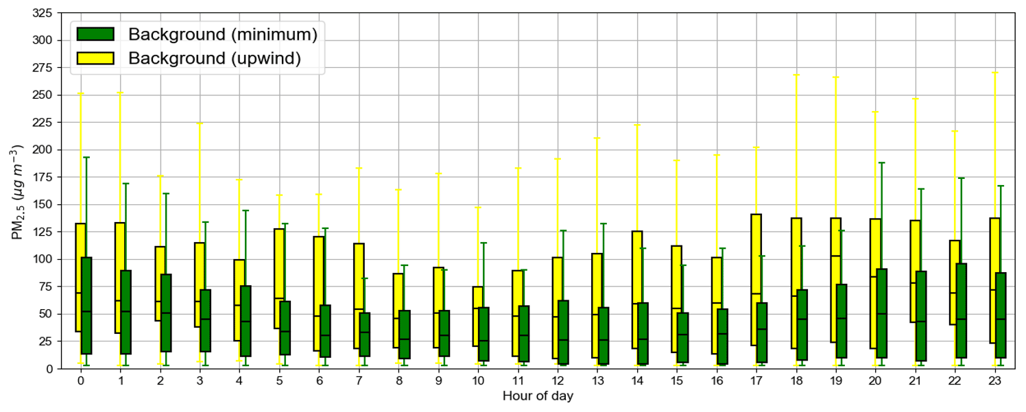
Figure 14Ranges in campaign period mean calculated background PM_2.5 concentrations for each hour of the day using minimum (green) and upwind (yellow) concentration methodologies.

Download

For each hour, the upwind background PM_2.5 upper quartile, median and lower quartile greatly exceed the corresponding values when using the minimum background methodology. This discrepancy is greatest for the upper quartile values and peaks during morning and evening rush hour, reaching ∼80 µg m⁻³ at 17:00 (Fig. 14). The lower whiskers, however, denoting the lowest datum lying within 1.5 times the interquartile range of the lower quartile, are common across both sets of PM_2.5 background diurnal cycles. Interpretation of these results is assisted by Fig. 15, which presents hourly wind vectors and PM_2.5 time series measurements throughout the campaign at all three upwind sites as well as urban sites 1 and 2. It is clear that the highest upwind PM_2.5 background concentrations occur when values at the additional site to the southeast of urban Beijing (site 14) are selected during periods of southerly winds (Fig. 15). The lowest background concentrations, therefore, can be attributed to either of the northerly sites (site 3 and site 10). Northerly winds advect clean air originating over the relatively unpolluted mountainous regions into urban Beijing (Tie et al., 2015). This switch in wind directions creates a saw-tooth pattern, with pollution episodes initially consisting of a slow build-up phase, associated with stagnant southerly winds, and culminating with sharp concentration drops related to the influx of cold northerly air (Li et al., 2017; Y. Wang et al., 2017). A clear example of this, from 23 to 27 November, is shown in Fig. 15.

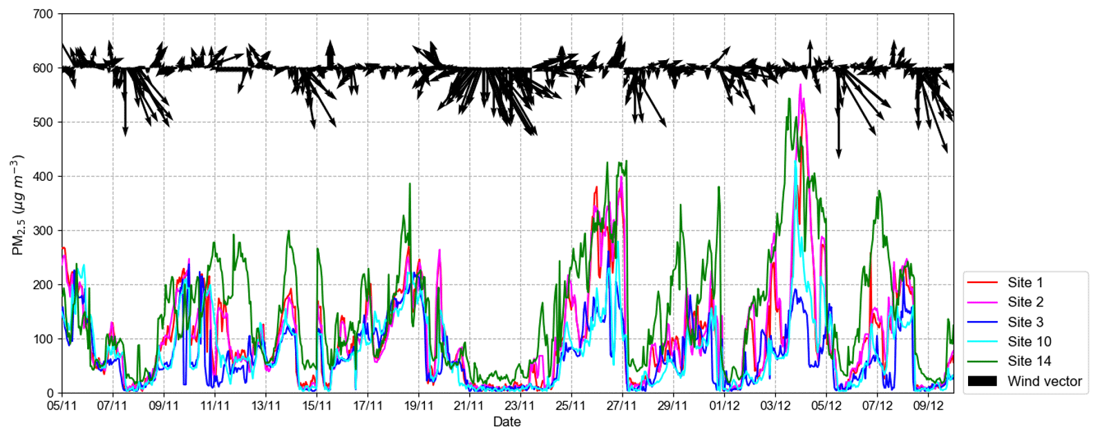
Figure 15Hourly PM_2.5 concentrations at measurement sites 1, 2, 3, 10 and 14 during the campaign period. Wind vectors, representing wind speed magnitude and direction recorded at the airport meteorological station, are also provided (black arrows).

Download

PM_2.5 concentrations at site 14, situated in the south-eastern corner of the model domain, are consistently higher than those measured at sites located in central Beijing. This monitoring station is located in the built-up Guangyang District of Langfang in Hebei province and is not in the immediate vicinity of any large point sources. Therefore, this region is possibly more heavily influenced by regional PM_2.5 advected from industrial towns and cities to the south. This highlights an important limitation of our study, which assumes a homogeneous background concentration for each species; this assumption may not be valid across such a large and complex urban area.

Both local PM_2.5 emission sources not represented in our study and background inhomogeneity appear to contribute substantially to differences in the spatial and temporal variation of measured and modelled PM_2.5 concentrations. However, the large diurnal variability in measured PM_2.5 concentration ranges across the domain (Fig. 13), not captured by the model, is more likely the influence of local emission sources, with longer timescales required for background PM_2.5 concentration variability driven by regional transport.

3.5 Impact of explicit road source modelling

In this section, we investigate the sensitivity of the simulated NO₂ concentrations to the inclusion of explicit road source emissions. Simulations that use aggregate 3-D grid sources alone are much less computationally expensive than those that also incorporate explicit road source emissions and allow studies to be performed with ADMS-Urban in urban areas where detailed road network information is unavailable. In Fig. 16, measured NO₂ concentrations averaged across the campaign are compared with those simulated using 3-D grid and explicit road sources, as well as 3-D grid sources only, derived from the MEIC Opt emissions inventory. By resolving road traffic emissions into explicitly represented road sources, as opposed to using gridded emissions only, mean modelled NO₂ concentrations across urban stations increase from 62.8 to 71.4 µg m⁻³ (Table 5). This modelled urban NO₂ concentration increase results in a Fb value improvement from −0.13 to 0 (Table 5) reflecting the greater NO₂ levels simulated by the model at locations in close proximity to explicit roads. By using grid sources only, the road traffic emissions are diluted over each 3×3 km grid cell and the strong concentration gradients associated with a region densely populated by major roads, illustrated in Fig. 4, are not captured. Similarly, Dédelé and Miskinyté (2015) and Hood et al. (2018) found that increased traffic emissions due to higher traffic volume and adjusted emission factors, respectively, produced improved Fb values using ADMS-Urban.

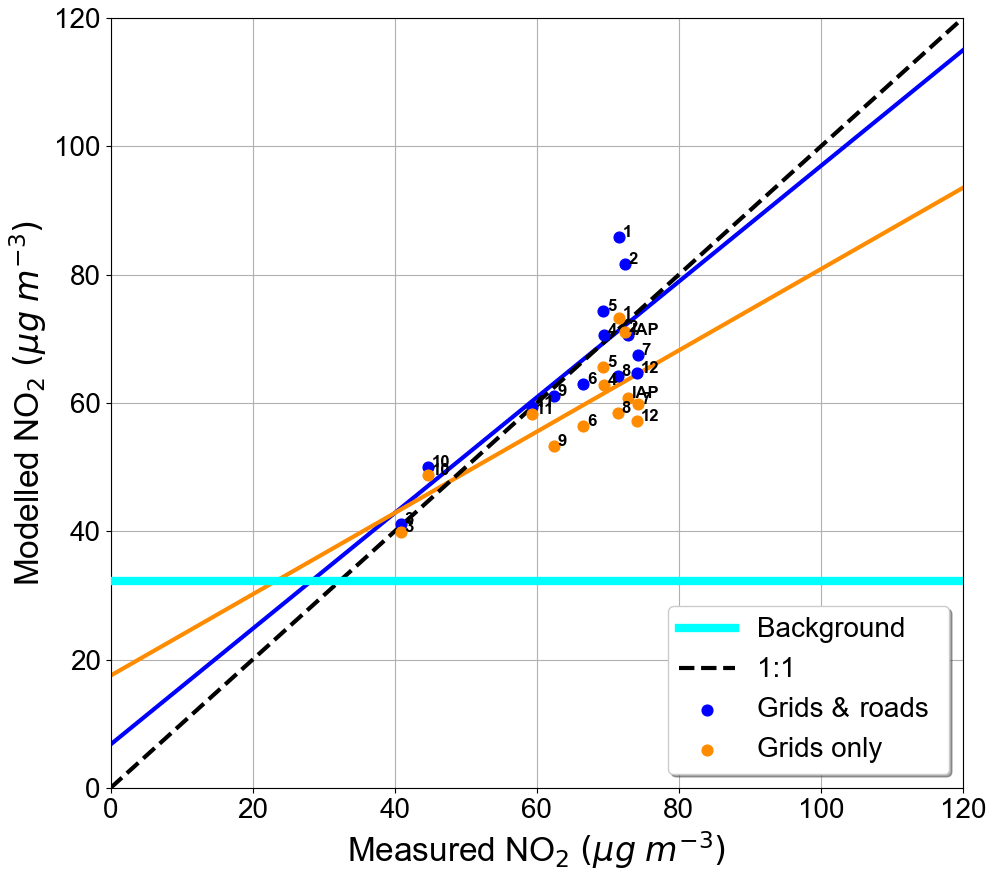
Figure 16Campaign period measured and modelled NO₂ concentrations at all the measurement sites (numbered). Modelled concentrations produced using 3-D grid and explicit road emission sources (blue) and 3-D grid sources only (orange) derived from the MEIC Opt emissions inventory. Horizontal light blue line represents campaign period mean background NO₂ concentrations calculated from measurements.

Download

Table 5Same information presented as in Table 4 but for NO₂ concentrations simulated (MEIC Opt) using 3-D grid sources only (G) as well as 3-D grid and explicit road sources (G-R) (also presented in Table 4).

Download Print Version | Download XLSX

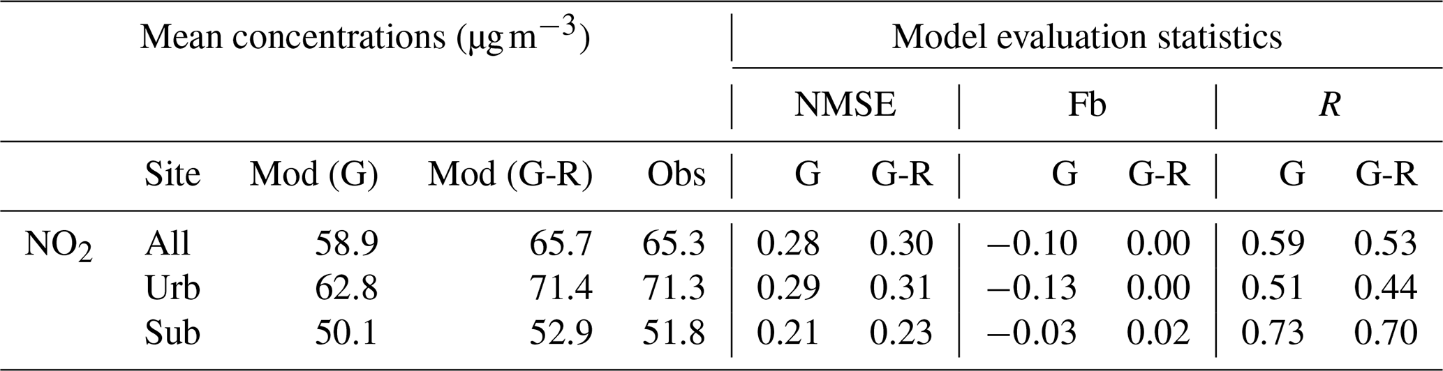
More accurate model predictions next to roads can lead to better assessments of human exposure levels to pollutant species and are evidence of the successful implementation of the top–down approach to estimating explicit road traffic emissions used in this study. However, it is also clear from Fig. 16 that agreement between modelled and measured NO₂ concentrations at sites 1 and 2 is substantially poorer when using explicit road sources than with the grid-source-only simulation. The model evaluation statistics for all monitoring sites (Table 5) reflect this with increases in NMSE from 0.28 to 0.3 and decreases in R from 0.59 to 0.53 when modelling road emissions explicitly. As discussed in Sect. 3.2, this highlights the impact that the assumption of constant traffic activity, high underlying gridded emissions or the absence of street canyon and urban canopy modelling can have on simulated concentrations at certain near-road locations.

Minimal R value changes and a much lower Fb improvement, −0.03 to 0.02, are seen across suburban compared to urban areas, following the inclusion of explicit road source emissions. This reflects the lower density of roads in suburban areas (Fig. 4) and therefore the absence of strong concentration gradients that enhance NO₂ levels at near-road urban locations. The relative influence of diffuse emissions contained within the underlying gridded emission sources on simulated pollutant concentrations is therefore more prominent with distance from Beijing's urban centre, with previous studies specifically highlighting the persisting importance of residential coal combustion for heating and cooking during winter in suburban and rural Beijing (Cai et al., 2018; Li et al., 2018).

3.6 Accounting for additional evening NO_x emission source

In this section, the influence of modifying the MEIC diurnal emissions profile, used for all previous simulations, to account for additional sources of nighttime NO_x emissions is examined. As discussed in Sect. 3.3, a likely explanation for the simulated underestimate in nocturnal NO_x and NO₂ concentrations is that an additional evening NO_x emission source is not accounted for in the emissions inventories. The timing of these peak NO₂ and NO_x measurements, between 23:00 and 06:00, coincides with the influx of HDDTs within Beijing's Fourth Ring Road.

Figure 17 presents the standard MEIC diurnal emissions profile (DP_MEIC), and two alternative profiles, DP_25 and DP_50, constructed by increasing the standard MEIC profile factors between 23:00 and 06:00 by ∼0.25 and ∼0.5, respectively, to account for additional nighttime HDDT emissions. For both modified emissions profiles, in order to retain the same 24 h emissions total, DP_MEIC is further adjusted between 07:00 and 22:00, by magnitudes that also preserve the timings of the morning and evening emissions peaks associated with rush hour traffic. The weekend emissions profile, characterised by a delayed morning peak and ∼30 % reduced total daily traffic emissions, is kept unchanged for all three sensitivity simulations.

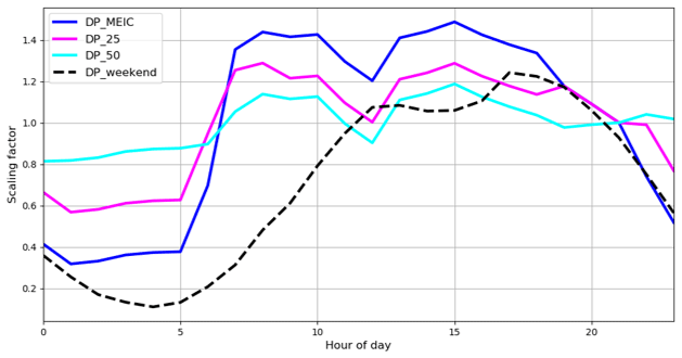
Figure 17Diurnal emissions profiles applied to the simulations shown in Fig. 18. Standard MEIC diurnal emissions profile (DP_MEIC) marked by blue line; modified DP_MEIC with increased proportions of nighttime emissions marked by pink (DP_25) and cyan (DP_50) lines and weekend emissions profile marked by dashed black line.

Download

Campaign period mean diurnal profiles of NO₂ concentrations, simulated using the diurnal emissions profiles shown in Fig. 17, are presented in Fig. 18. At suburban site 11, the close agreement between simulated and measured NO₂ concentrations using DP_MEIC is strengthened further by increasing the proportion of emissions released at night relative to the daytime. Modelled NO₂-level overestimations throughout the morning and afternoon hours at sites 12 and IAP using DP_MEIC are reduced when applying the two modified emissions profiles. However, at site 1 the application of DP_50 is unable to reduce daytime NO₂ concentrations substantially, which is likely related again to the effect of overestimated emissions along the nearest explicit road source (Fig. 8). The evening NO₂ concentration is underestimated at sites 1, 12 and IAP, using DP_MEIC, and this is successively reduced by a small amount with DP_25 and DP_50. The remaining evening differences suggest that, although the inclusion of higher nighttime emissions improves agreement, other possible issues exist related to ADMS-Urban's inability to model dispersion at very low wind speeds; inaccurate underlying gridded emissions; the simplified GRS chemistry scheme; and the exclusion of street canyon and urban canopy modelling or PBL dynamics.

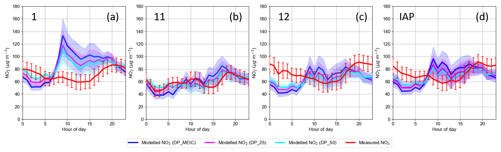
Figure 18Campaign period mean diurnal variation in measured and modelled NO₂ concentrations using MEIC Opt at sites (a) 1, (b) 11, (c) 12, and (d) IAP. Measurements marked by red line. Shaded areas and error bars represent the 95 % confidence intervals for simulated and measured concentrations, respectively.

Download

3.7 The influence of boundary layer height and stability on diurnal NO₂ concentrations

In this section, the impact of PBLH and stability on diurnal NO₂ concentrations is explored with further sensitivity simulations. The space into which emitted plumes of pollutants can disperse and mix is determined by the PBLH. Figure 19 shows the difference between measured and modelled PBLHs and their impact on simulated diurnal NO₂ concentrations. Differences between the PBLH simulated without evening stability adjustment and the observed PBLH (Fig. 19) are characterised by a daytime overprediction and nighttime underprediction. At 15:00, the rapidly growing convective PBL peaks at ∼1100 m, exceeding the observed heights by ∼200 m. This difference between observed and simulated PBLHs could be a result of an overestimation of the solar radiation-driven surface sensible heat flux and mechanically driven turbulent flux values, which are the principal parameters impacting the modelled PBLH. Additionally, due to complex cloud physics, detecting the exact limit of vertical mixing is difficult in the presence of low-level stratiform clouds, which form frequently in Beijing during winter, and may further account for low PBLHs derived from ceilometer observations (Kotthaus and Grimmond, 2018). After sunset at 17:00, the modelled PBLH shrinks to ∼200 m, 400 m below the measured height. This sharp transition between an unstable and a stable modelled PBL is a consequence of ADMS-Urban not accounting for the UHI effect in its surface energy balance calculations, as described in Sect. 2.1.2.

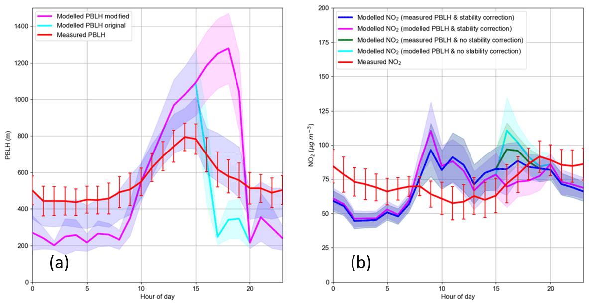
Figure 19(a) Campaign period mean diurnal variation in modelled PBLH with stability correction (pink), modelled PBLH without stability correction (cyan) and measured PBLH (red). (b) Campaign period mean diurnal variation in measured (red) and modelled NO₂ concentrations with measured PBLH and stability correction (blue), modelled PBLH with stability correction (pink), measured PBLH without stability correction (green), and modelled PBLH without stability correction (cyan) at the IAP field site. Shaded areas and error bars represent the 95 % confidence intervals for simulated and measured PBLH and concentrations, respectively.

Download

The early evening stability adjustment (Sect. 2.1.2) applied to all previous simulations in this study replicates the effect of the UHI by reducing PBL stability between 16:00 and 19:00. By applying the stability modification, early evening modelled PBLH increases and reaches ∼1300 m by 18:00 before sharply decreasing to ∼200 m by 20:00. Note that directly input PBLH measurements are unaffected by changes to L_MO and surface heat flux terms. The stability adjustment reduces NO₂ concentrations simulated at 16:00 using modelled and measured PBLHs by ∼40 and ∼15 µg m⁻³, respectively, greatly improving agreement with measurements. The sharp morning modelled NO₂ concentration rise, peaking at 09:00, decreases by ∼10 µg m⁻³ through use of the measured PBLH alone. However, application of a similar PBL stability adjustment, between 07:00 and 10:00, would likely reduce the early morning PBLH underestimation and further weaken the modelled NO₂ concentration rise associated with the input of rush hour-related NO_x emissions into a morning PBL that is currently too stable and too shallow compared to observations.

The results suggest that although atmospheric stability modifications have a strong impact on NO₂ concentrations, the use of observed PBLH instead of modelled heights has little effect. This is clearest outside the hours in which the stability correction has been applied, when large (∼300 m) measured and modelled mid-afternoon and nighttime PBLH discrepancies have negligible impact on simulated NO₂ concentrations. The greater impact of PBL stability changes alone, however, is clearly evidenced by the ∼15 µg m⁻³ difference at 16:00 between simulations using measured PBLHs with and without the stability correction. This dominant influence of PBL stability is possibly related to the impact in the model configuration of near-surface traffic emissions and the exclusion of elevated point sources, with pollution dispersion from the latter more likely to be restricted by low PBLHs which would then further affect modelled NO₂ levels.