the Creative Commons Attribution 4.0 License.
the Creative Commons Attribution 4.0 License.
 | 05 Mar 2020
The diurnal stratocumulus-to-cumulus transition over land in southern West Africa
Xabier Pedruzo-Bagazgoitia
Stephan R. de Roode
Bianca Adler
Karmen Babić
Cheikh Dione
Norbert Kalthoff
Fabienne Lohou
Marie Lothon
Jordi Vilà-Guerau de Arellano
The misrepresentation of the diurnal cycle of boundary layer clouds by large-scale models strongly impacts the modeled regional energy balance in southern West Africa. In particular, recognizing the processes involved in the maintenance and transition of the nighttime stratocumulus to diurnal shallow cumulus over land remains a challenge. This is due to the fact that over vegetation, surface fluxes exhibit a much larger magnitude and variability than on the more researched marine stratocumulus transitions. An improved understanding of the interactions between surface and atmosphere is thus necessary to improve its representation. To this end, the Dynamics-aerosol-chemistry-cloud interactions in West Africa (DACCIWA) measurement campaign gathered a unique dataset of observations of the frequent stratocumulus-to-cumulus transition in southern West Africa. Inspired and constrained by these observations, we perform a series of numerical experiments using large eddy simulation. The experiments include interactive radiation and surface schemes where we explicitly resolve, quantify and describe the physical processes driving such transition. Focusing on the local processes, we quantify the transition in terms of dynamics, radiation, cloud properties, surface processes and the evolution of dynamically relevant layers such as subcloud layer, cloud layer and inversion layer. We further quantify the processes driving the stratocumulus thinning and the subsequent transition initiation by using a liquid water path budget. Finally, we study the impact of mean wind and wind shear at the cloud top through two additional numerical experiments. We find that the sequence starts with a nighttime well-mixed layer from the surface to the cloud top, in terms of temperature and humidity, and transitions to a prototypical convective boundary layer by the afternoon. We identify radiative cooling as the largest factor for the maintenance leading to a net thickening of the cloud layer of about 18 g m−2 h−1 before sunrise. Four hours after sunrise, the cloud layer decouples from the surface through a growing negative buoyancy flux at the cloud base. After sunrise, the increasing impact of entrainment leads to a progressive thinning of the cloud layer. While the effect of wind on the stratocumulus layer during nighttime is limited, after sunrise we find shear at the cloud top to have the largest impact: the local turbulence generated by shear enhances the boundary layer growth and entrainment aided by the increased surface fluxes. As a consequence, wind shear at the cloud top accelerates the breakup and transition by about 2 h. The quantification of the transition and its driving factors presented here sets the path for an improved representation by larger-scale models.


Stratocumulus (Sc) clouds play a critical role in the radiative balance of the planet given their high albedo (Hartmann et al., 1992; Chen et al., 2000) and extensive cover worldwide (Eastman and Warren, 2014; Eastman et al., 2014). These boundary layer clouds are a common feature in southern West Africa (SWA) and recur in the night and morning during the monsoon season between May and September (van der Linden et al., 2015; Hill et al., 2018). Possible future changes in highly sensitive Sc forcings in SWA, such as anthropogenic regional aerosol increase (Boucher et al., 2013) or the global CO2 rise (Schneider et al., 2019), further motivate a better understanding of the boundary layer cloud dynamics over land in SWA.
During the monsoon season, the intertropical convergence zone shifts northward till 15∘ N, facilitating the extension of the maritime air masses inland. The arrival of the cooler, but not necessarily moister, mass of air more than a 100 km inland facilitates the onset of Sc clouds over land (Adler et al., 2019; Babić et al., 2019; Dione et al., 2019). The fact that this mass of air is characterized by cloudless conditions when over the sea reveals the importance of the land and other local factors for the cloud formation and maintenance (Adler et al., 2019; Babić et al., 2019; Lohou et al., 2019). Lohou et al. (2019) extended the previous work and summarized the four phases leading from cloud formation to dissipation: stable phase, jet phase, stratus phase and convective phase. In addition, they described three observed scenarios for the breakup and dissipation of the Sc deck throughout the day. Such scenarios differed for the Sc coupling to surface and for the presence of convective clouds below the Sc.
The high albedo of low-Sc clouds and their misrepresentation by most climate models lead to significant biases in the regional surface energy balance, especially if the evolution and spatial structure of the cloud field is not correctly represented (Hannak et al., 2017). More specifically, the maintenance, dissipation or transition to other cloud forms of the Sc cloud layer after sunrise have strong implications for the regional energy balance (Knippertz et al., 2011; Hannak et al., 2017; Lohou et al., 2019). These biases are less relevant during the night due to the absence of shortwave radiation, as cloud-induced variations in the longwave radiation are 1 order of magnitude smaller than those of shortwave radiation. To improve our understanding and to better quantify the effects of Sc clouds over land in an observation-scarce region, the Dynamics-aerosol-chemistry-cloud interactions in West Africa (DACCIWA) project deployed an extensive network of observations during June and July in 2016 comprising three fully instrumented supersites (Knippertz et al., 2015; Flamant et al., 2018; Kalthoff et al., 2018). The resultant dataset with high spatio-temporal observations of the cloud transition allows us to tackle two important questions. Firstly, it allows us to understand the transition (Lohou et al., 2019) and, using idealized numerical simulations, reproduce a characteristic stratocumulus-to-cumulus (Sc–Cu) transition with typical conditions of SWA. Secondly, we aim at identifying the physical processes and their complex interplay that leads to a breaking-up of the Sc deck.
Here, we extend the impacts of the land–atmosphere interactions on the Sc–Cu transition and breakup. Previous studies have largely relied on high-resolution explicit modeling, e.g., large eddy simulation (LES), of marine Sc clouds. Over the sea, surface fluxes are low and show little diurnal variation. Evaporation from the sea provides the necessary moisture to maintain the Sc layer, which is well-mixed from top cloud down to the surface by the turbulence generated at the cloud top by radiative cooling (Wood, 2012). Transitions from Sc to shallow cumulus have also been studied through LES mostly in maritime conditions (Bretherton et al., 1999a; Sandu and Stevens, 2011; de Roode et al., 2016). Such transitions are typically investigated using a Lagrangian approach in which the trajectory of an air mass is followed as it is advected from the subtropics towards the Equator. An increasing sea surface temperature and decreasing subsidence are usually imposed along the trajectory, leading to increasing latent heat fluxes and boundary layer height, respectively. The main mechanism for such transitions over the sea is the increase in buoyancy along the cloud layer by higher latent heat flux, leading to larger entrainment velocities aided by the subsidence decrease, and the eventual dissipation of the Sc cloud layer. Over land, however, such transitions may have different drivers, given their differently partitioned surface fluxes as well as their larger magnitude and diurnal variability than over the sea. Ghonima et al. (2016) performed a thorough idealized LES study on Sc–Cu transitions both over land and over the sea. They based all their cases on vertical profiles of mid-latitude marine conditions and prescribed different Bowen ratios to regulate the surface fluxes over land. They found that the Bowen ratio determines whether the surface fluxes lead to a thinning or thickening of the cloud layer. This was proved by a set of systematic experiments. Furthermore, they provided a set of Bowen ratio-dependent feedbacks highlighting the relevant role of the land: one feedback loop where the increase in sensible heat flux would increase entrainment, thinning the cloud layer, enhancing the net radiation at the surface and further increasing the sensible heat flux. They provided two more feedbacks related to latent heat flux (LE): one in which its increase moistens and thickens the cloud layer, decreasing net radiation and surface and, consequently, LE; and another in which the LE increase enhances entrainment, leading to cloud thinning and a further increase in LE. In contrast to mid-latitude marine conditions, atmospheric conditions in near-equatorial SWA are characterized by a moister and warmer atmosphere as well as stronger solar irradiation and, locally, larger evapotranspiration. These differences pose the question of whether the mechanisms and physical processes identified by Ghonima et al. (2016) remain relevant for SWA.
Our study thus aims at filling the knowledge gap on turbulence-resolving numerical experiments of Sc–Cu transitions taking place over land and, specifically, in subtropical atmospheric conditions. We systematically focus on the following processes and the role played in the maintenance of the Sc and its transition to cumulus clouds: radiation, entrainment and the land surface fluxes. Net longwave radiation is the source for cloud maintenance during the night through cloud top cooling. As the day progresses, increasing shortwave radiation becomes a factor for dissipation. Entrainment is known to affect the cloud layer by drying and warming it, raising it and weakening the thermal inversion. The land surface fluxes respond to variations in wind and radiation and affect the transport of heat and moisture to the cloud layer as well as the entrainment. In addition, we briefly study the evolution of metrics frequently used by parameterizations in larger-scale models in the Sc–Cu transition.
Finally, during the DACCIWA campaign a recurrent low-level jet along the cloud layer was observed (Adler et al., 2019; Dione et al., 2019), raising an additional question regarding the effects of wind shear on Sc and its transition (Lohou et al., 2019). Previous work on modeled sheared Sc over the sea suggests that shear at the cloud top lowers the water content of Sc by enhancing the entrainment rate (Wang et al., 2008, 2012). Mechem et al. (2010) presented a land Sc case and briefly studied the effects of shear. They similarly concluded that in the presence of cloud top wind shear, entrainment velocity increases, leading to a decrease in cloud liquid water content. However, to the best of our knowledge, there is no work studying the effects of wind shear on stratocumulus-to-cumulus transitions. Thus, we additionally perform some sensitivity studies on the effect of wind and wind shear at the cloud top on the Sc–Cu transition.
Our research seeks to answer these three research questions:
-
How is a stratocumulus-to-cumulus transition over land characterized? What is the relevance of the local processes?
-
How do the contributions of each physical process vary with time during the maintenance, thinning and transition of the cloud layer?
-
How do these high-resolution simulations quantify metrics relevant for larger-scale models during the transition?
2.1 Dutch Atmospheric Large Eddy simulation
To explicitly resolve the Sc–Cu transition we perform our numerical experiments using the Dutch Atmospheric Large Eddy Simulation (DALES) (Heus et al., 2010; Ouwersloot et al., 2016). LES models explicitly resolve most of the energy-containing turbulent motions in the boundary layer, including the stratocumulus and shallow cumulus cloud dynamics. Based on the initial work of Nieuwstadt and Brost (1986), DALES is an LES model that has been used individually or within a model intercomparison for a broad range of cases, from clear-sky diurnal cycles (Pino et al., 2003) to boundary layers topped by stratocumulus (Blossey et al., 2013; van der Dussen et al., 2015) or cumulus (Siebesma et al., 2003; Vilà-Guerau de Arellano et al., 2014), including Sc–Cu transitions over the sea (van der Dussen et al., 2013; de Roode et al., 2016). Here, we use the DALES 4.1 version. We describe below the relevant parameterizations for this study.
-
An interactive land surface model with a mechanistic representation of plant behavior. It regulates the surface latent, and sensible heat fluxes, as well as the CO2 flux depending on environmental variables such as CO2 concentration, atmospheric vapor pressure deficit, temperature, soil moisture and surface wind (Jacobs and de Bruin, 1997; van Heerwaarden et al., 2010; Vilà-Guerau de Arellano et al., 2015). It is upgraded with a two big-leaf (sunlit and shaded leaves) scheme allowing for different penetration rates of direct and diffuse radiation along the canopy (Pedruzo-Bagazgoitia et al., 2017). The fact that surface fluxes are higher and more variable over land, responding to environmental variables and potentially altering the boundary layer and cloud structure, explains the need for an interactive scheme such as the one presented here. Further details on the settings of the land surface scheme are presented in Sect. 2.3.
-
The two-stream radiation scheme Rapid Radiative Transfer Model for use in GCMs (RRTMG; Iacono et al., 2008). It is used to provide longwave and direct and diffuse shortwave radiation at each grid box depending on liquid water and other chemical compounds. This scheme allows us to represent the surface dynamic heterogeneities caused by cloud spatial inhomogeneities, as it provides a column-dependent net radiation at the surface.
-
The microphysics scheme by Khairoutdinov and Kogan (2000), specifically designed for Sc clouds. It includes cloud-droplet sedimentation, found to be highly relevant in the representation of Sc clouds (Ackerman et al., 2004; Bretherton et al., 2007; Dearden et al., 2018).
The subgrid turbulence is parameterized using a turbulence kinetic energy (TKE) model following Deardorff (1980). Fifth- and second-order schemes are used to compute the advection over horizontal and vertical directions, respectively. The integration of the governing equations over time is carried out using a third-order Runge–Kutta scheme. For a deeper insight in the mentioned numerical settings, the reader is referred to Heus et al. (2010). In particular, Eqs. (25), (43) and (49).
2.2 Observations
We base our idealized study on observations taken during the field campaign of the DACCIWA project during the months of June and July 2016. We focus on the observations of 26 June 2016 at the Savè supersite. On this day a stratocumulus deck was observed during the night and morning above Savè, followed by a cloud base rise and breakup during the late morning and afternoon (Dione et al., 2019). We briefly describe below the methods and observations used to inspire our idealized study. For a fully detailed explanation of the observations and the dataset, the reader is referred to Kalthoff et al. (2018) and Bessardon et al. (2020), respectively.
-
Radiosondes were performed with the MODEM radiosounding system. The temperature and relative humidity of the air were measured with a 1 s temporal resolution (≃ 4–5 m in vertical resolution). The wind speed, direction and the pressure were determined based on the radiosonde GPS coordinates (Derrien et al., 2016).
-
The cloud base height is measured by a continuously running ceilometer measuring backscatter profiles with a 1 min resolution. Three cloud base heights are obtained from the backscatter profiles using the manufacturer algorithm. We select the lowest cloud base to ensure that the detection reflects a cloud base and not, for example, a cloud edge. The data are available at Handwerker et al. (2016).
-
The cloud top height is measured by a dual-polarized cloud radar, which allows us to distinguish between hydrometeors and other targets. The cloud top height is estimated from the 5 min averaged reflectivity profiles of hydrometeors applying a threshold of −35 dBz (Bauer-Pfundstein and Goersdorf, 2007). Therefore, reflectivities larger than −35 dBz are considered clouds. The data are available at Handwerker et al. (2016).
-
The cloud cover is calculated as the percentage of cloud base height measurements below 1000 m (Adler et al., 2019; Zouzoua, 2020). The values are averaged over 19 d of the campaign to prevent too high a variability by single point observations at individual days.
-
The surface fluxes and net radiation are obtained from an energy balance station deployed over a mix of grass and bushes. The 30 min sensible and latent heat fluxes are calculated from high-frequency (20 Hz sampling rate) measurements of wind speed and sonic temperature obtained by ultrasonic anemometer and humidity measurements which are based on the absorption of near-infrared radiation and obtained by a fast-response LI-COR sensor by applying eddy-correlation method (Mauder et al., 2013). The data are available at Kohler et al. (2016).
-
The two sets of turbulent kinetic energy measurements are calculated from the anemometer measurements of wind speed at 4 and 7.8 m by two energy balance stations deployed over a mix of grass and bushes and over corn, respectively.
2.3 Model settings and initial conditions
Constrained by the surface and upper-atmospheric observations, we design an academic case to be simulated through LES. Our aim, by means of an idealized numerical experiment, is to simulate a Sc–Cu transition, including the Sc breakup, during typical atmospheric conditions in SWA rather than the reproduction of an exact day that occurred during the DACCIWA measurement campaign. In particular, we study the Sc–Cu transition of a coupled case or Scenario 1 as described in Lohou et al. (2019).

Figure 1Vertical profiles of potential temperature (a), total specific humidity (b) and wind (c) as observed through radiosondes (at 00:00, 06:00 and 09:00 UTC from black to light grey) on 26 June 2016 and as prescribed in the idealized LES experiments (red and blue). The three experiments REF, MEAN and SHEAR differ only in the prescribed wind profiles.
We design a 12 × 12 km2 wide and 3.2 km high domain, with a grid box size of 50 × 50 × 4 m3 resulting in 800 vertical levels. Such high vertical resolution is required in order to reduce the overestimation of mixing and entrainment typical of coarser LES simulations with Sc (Bretherton et al., 1999b; Stevens et al., 2005). Although at this vertical resolution, processes such as evaporative cooling and cloud top mixing might still be overestimated (Stevens et al., 2005; Mellado, 2017), a much finer resolution, or a direct numerical simulation approach, would not allow computationally for an integrated simulation of both cloud top and ground surface. As will be shown later, both interfaces play a critical role in the development and transition studied here. We use periodic boundary conditions on the horizontal directions. We start the experiment at 03:30 UTC to allow for 1 h of spin-up of the Sc layer and end the experiment at 18:30 UTC after sunset.
The vegetation near and around the site consisted of heterogeneous patches containing shrubs, crops or taller trees in very dense thickets with areas in the order of 50–100 m, a size too small to lead to the formation of secondary circulations (Patton et al., 2005). Unfortunately, no detailed measurements were taken on the vegetation types and properties during the DACCIWA campaign. Thus, the case presented here shows spatially homogeneous soil and vegetation properties and is constrained taking into account the information available on the surface fluxes. The land surface model allows for spatially heterogeneous values of the surface fluxes depending on environmental conditions. This is known to be essential to realistically simulate clear (Patton et al., 2005) and cloudy (Sikma and Vilà-Guerau de Arellano, 2019) convective boundary layers. The terrain around the measuring site was relatively flat (Adler et al., 2019), allowing us to assume a topography-free domain. Thus, assuming a flat and homogeneous surface simplifies our study and permits us to focus on the local effects that can be more easily generalized to similar situations in SWA. Meanwhile, the dynamic heterogeneities created guarantee a sufficiently realistic representation of the boundary layer during the day.
We prescribe a subsidence profile, following Bellon and Stevens (2012), of the shape , with w0=5.3 mm s−1 and zw=300 m. Such a profile translates into mm s−1 at the initial cloud top height of 570 m. Our choice for the subsidence profile was such that it would keep a nearly constant cloud top height during the night, and it is justified given the uncertainty and high temporal variability in subsidence profiles, as well as its large spread among regional simulations carried out with the Consortium for Small-Scale Modeling (COSMO) within the DACCIWA project or ERA-interim. For simplicity we assume the subsidence profile to be constant during the entire simulation. To limit the complexity of our idealized experiments and focus on the interaction of the surface and boundary layer processes, we prescribe no advection of heat or moisture at any height. Adler et al. (2019) and Babić et al. (2019) found cold air advection necessary for the formation of the cloud layer. Yet its relevance decreased as sunrise approached, thus justifying our assumption.
For all the experiments we calculate the vertical profiles of the radiative fluxes every minute. In doing so, we quantify how radiative fluxes are perturbed by the liquid water related to cloud dynamics and how they interact with the surface. This is done to account for fast fluctuations of net radiation at the cloud top and surface. The latter is relevant given its potential to alter surface fluxes and, thus, the evolution of the boundary layer and clouds (Vilà-Guerau de Arellano et al., 2014; Gronemeier et al., 2016; Sikma and Vilà-Guerau de Arellano, 2019). Based on aircraft observations during the DACCIWA campaign (Taylor et al., 2019), the cloud droplet number concentration is set to 300 cm−3 and remains constant throughout the experiment. No radiative effects of aerosols are taken into account here.
We show in Fig. 1 the vertical profiles obtained through three radiosondes during the night and morning of 26 June 2016. The radiosonde at 06:00 UTC, the closest to our initialization time, shows a strong increase in potential temperature of about 3 K at 570 m high. Above, all radiosondes show similar temperature lapse rates of about 4.6 K km−1. Subtropical marine Sc clouds are frequently capped by much drier air above the cloud top (Duynkerke et al., 2004; Wood, 2012). Yet none of the radiosonde profiles show any strong jump in moisture above 570 m. If anything, they show a humidity increase above the cloud layer. Such an increase could be related to the previously questioned reliability of radiosonde measurements as they exit the cloud layer during their ascension (Lorenc et al., 1996; Mechem et al., 2010; Babić et al., 2019). Situations without a dry jump above the Sc cloud top have been previously reported over land (Mechem et al., 2010) and are more typical of arctic climates (Morrison et al., 2012).
The observations demonstrate that the idealized experiment's initial conditions lie within typical meteorological conditions in SWA. The initial idealized profiles prescribe a well-mixed layer up to 570 m with liquid water potential temperature θl=296 K and specific humidity qt=15.5 g kg−1. Such thermodynamic conditions result in a domain-covering cloud layer from 226 to 570 m high, topped by a jump of 4.5 K in temperature, but without a jump in specific humidity. Above 570 m the potential temperature and total moisture idealized profiles exhibit constant slopes of 4.67 K km−1 and 3.29 g kg−1 km−1, respectively. Given the spread in vertical profiles by radiosondes, we performed additional simulations exploring variations in the profiles of 0.5 K and 0.5 g kg−1. Results showed a very similar development of the Sc–Cu transition.
Our reference experiment REF prescribes no wind at any heights. To study the effect of wind and wind shear, we perform two additional numerical experiments – MEAN and SHEAR – where we account for different idealized wind effects. This sensitivity analysis is motivated by the recurrent winds with the shape of low-level jet, such as those in Fig. 1c, that were frequently observed during the DACCIWA campaign (Kalthoff et al., 2018; Adler et al., 2019; Dione et al., 2019). Failed attempts to maintain a low-level jet-like wind profile together with the Sc cloud layer in preliminary experiments suggest that the jet-like wind is the result of large-scale dynamics and, thus, beyond the scope of the present study on local factors. The large-scale origin of the low-level wind is also supported by more detailed observational analysis (Babić et al., 2019; Adler et al., 2019; Dione et al., 2019). Following our idealized approach, the initial wind speed and wind direction are inspired by the observations and adapted to better study how these effects influence the Sc–Cu transition. In this case, the mean wind and the shear at the cloud top are considered. We prescribe a constant horizontal wind of 3 m s−1 along the whole vertical profile in MEAN based on above-cloud-layer radiosonde observations (Fig. 1c). Consistent with our idealized setting, we assume the wind to blow only along the x direction and without prescribed directional shifts with height. In SHEAR we add a jump of 5 m s−1 to the mean 3 m s−1 at the cloud top to represent a wind shear of a similar magnitude as the observed low-level jet. The values prescribed here for the simplified effects of the low-level jet are representative not only of the day studied here but also of the whole measurement campaign (Dione et al., 2019). The free-troposphere wind shows a constant increase of 5 m s−1 km−1 in SHEAR. Our aim here is to maintain a shear contribution as the cloud layer rises. We prescribe geostrophic winds identical to the initial wind profiles, as the goal is to observe the impact of wind on the transition and not vice versa. In summary, differences between MEAN and REF serve in identifying the role played by a mean wind, which will mainly enhance the surface fluxes. MEAN and SHEAR differences show the impact of the local shear at the cloud top.
To determine the dependency of the results on the Galilean transformation, we performed two extra simulations. We reproduced the MEAN experiment with an additional grid translation of 3 m s−1 identical to the prescribed mean wind, and the SHEAR experiment with a grid translation of 6 m s−1. These additional experiments yielded very similar results to the original ones and confirmed the independence of our numerical experiments on this condition. Therefore, for the sake of simplicity none of the simulations shown here have Galilean transformation prescribed.
3.1 Evolution of the transition
Figure 2 shows the diurnal evolution of cloud height, cover and liquid water path (LWP) and their connection with surface turbulent fluxes in the REF simulation. It also includes the observations corresponding to the day by which our case is inspired. At Fig. 2a both cloud top and base remain approximately constant for the first hours. The LWP values are at the high end of domain-average LWP for marine stratocumulus cloud (Wood, 2012) and coincide with observed ones during the DACCIWA campaign (Babić et al., 2019; Kalthoff et al., 2018). The initially constant cloud top height coincides with the boundary layer height. As a result, the boundary layer height evolution can be expressed using mixed layer theory by the relation that equates the entrainment velocity and the subsidence. Assuming horizontally homogeneous conditions, it reads (Lilly, 1968)
with h the boundary layer height defined as the height of minimum buoyancy flux, we the entrainment velocity and wsubs(h) the subsidence, depending on height as described in Sect. 2.3, at h. For this experiment and before sunrise cm s−1, which is in the same order of magnitude as previously reported nocturnal marine Sc cases (Stevens et al., 2003). Between 2 to 3 h after sunrise (06:00 UTC) the cloud layer begins to rise and subsequently decreases its liquid water content (Fig. 2b), allowing more radiation to reach the surface and enhancing the surface fluxes (see Rnet, LE and SH increase between 06:00 and 10:00 UTC in Fig. 2c). During this time the domain-average cloud base cbase_avg follows the observed cloud base and so do the surface fluxes with the observed ones. The onset of the convective phase, defined by Lohou et al. (2019) as the time when the sensible heat flux SH>10 W m−2, takes place between 07:00 and 07:30 UTC according to observations and at 06:55 UTC in REF. The breakup in the cloud layer, defined as the time when cloud cover (cc) is below 1, takes place at around 11:30 UTC in the LES experiment and coincides with the observed sharp increase in surface fluxes of about 150 W m−2, i.e., a 3-fold increase compared to before-breakup values. This sudden change coincides with the sharp increase in net radiation due to cloud breakup (see Fig. 2c) and reveals that surface fluxes are radiation-driven at this stage. The good agreement in the surface flux partitioning as modeled and observed justifies the use of a land surface model sensitive to several environmental variables at the surface (see Sect. 2.1). After 11:30 UTC observations show large variability in measured cloud base heights (Fig. 2a), suggesting either the presence of shallow clouds below the Sc cloud layer or the breakup of the Sc layer (Lohou et al., 2019). Therefore, the jump in cloud base height from about 1000 to 500 m is due to either the appearance of the first shallow cumulus at 500 m after the stratocumulus cloud base rises up to 1000 m or to the breakup of the stratocumulus deck leading to different observed cloud base heights. About 90 min after cloud breakup, cc decreases quasi-linearly until the end of the simulation. The same pattern for cloud cover is shown by observations, although 1 h earlier. Note, however, that the observations of cc are averaged over 19 d selected due to cloud onset happening before 04:00 UTC (Zouzoua, 2020). The variability between the days considered in the average also explains the cc values below 1 before 06:00 and after 08:30 UTC.
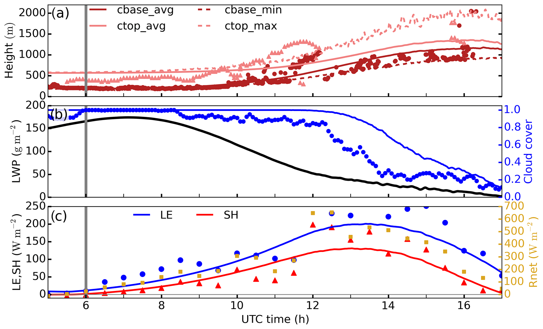
Figure 2Time series of the domain-average cloud base (cbase_avg as solid dark red line) and cloud top (ctop_avg as solid light red line), maximum cloud top (ctop_max in dashed light red line) and minimum cloud base (cbase_min in dashed dark red line) (a), liquid water path and cloud cover (b), and latent and sensible heat fluxes as well as net radiation (c) in REF. Observed cloud base and cloud top heights on 26 June are represented by dark red circles and light red triangles, respectively, in (a). Observed cloud cover, averaged over 19 campaign days is shown in blue circles in (b). Observed latent and sensible heat fluxes are shown by blue circles and red triangles, respectively, and net radiation in yellow squares in (c). The vertical grey lines indicate the sunrise time.
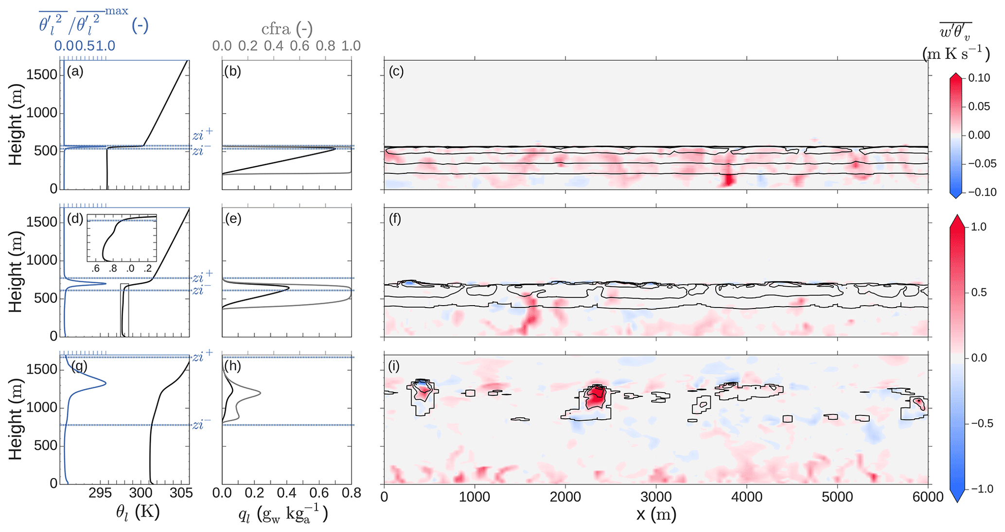
Figure 3On the left (a, d, g), slab-averaged vertical profile of liquid potential temperature θl (black) and normalized over its maximum value (blue). The inversion layer upper zi+ and lower zi− limits are indicated by dashed blue horizontal lines. In the center (b, e, h) slab-averaged vertical profiles of liquid water mixing ratio ql (black) and horizontal cloud fraction cfra (grey). On the right (c, f, i), horizontal cross section of buoyancy flux (red (blue) indicating upwards (downwards) movement of buoyantly positive (negative) air) and cloud liquid water (in black contour lines every 0.3 gw kg). Panels (a), (b) and (c) correspond to 05:00 UTC, (d), (e) and (f) to 11:00 UTC, and (g), (h) and (i) to 14:30 UTC. The inset in (d) is an expanded version of the rectangle in the same panel.
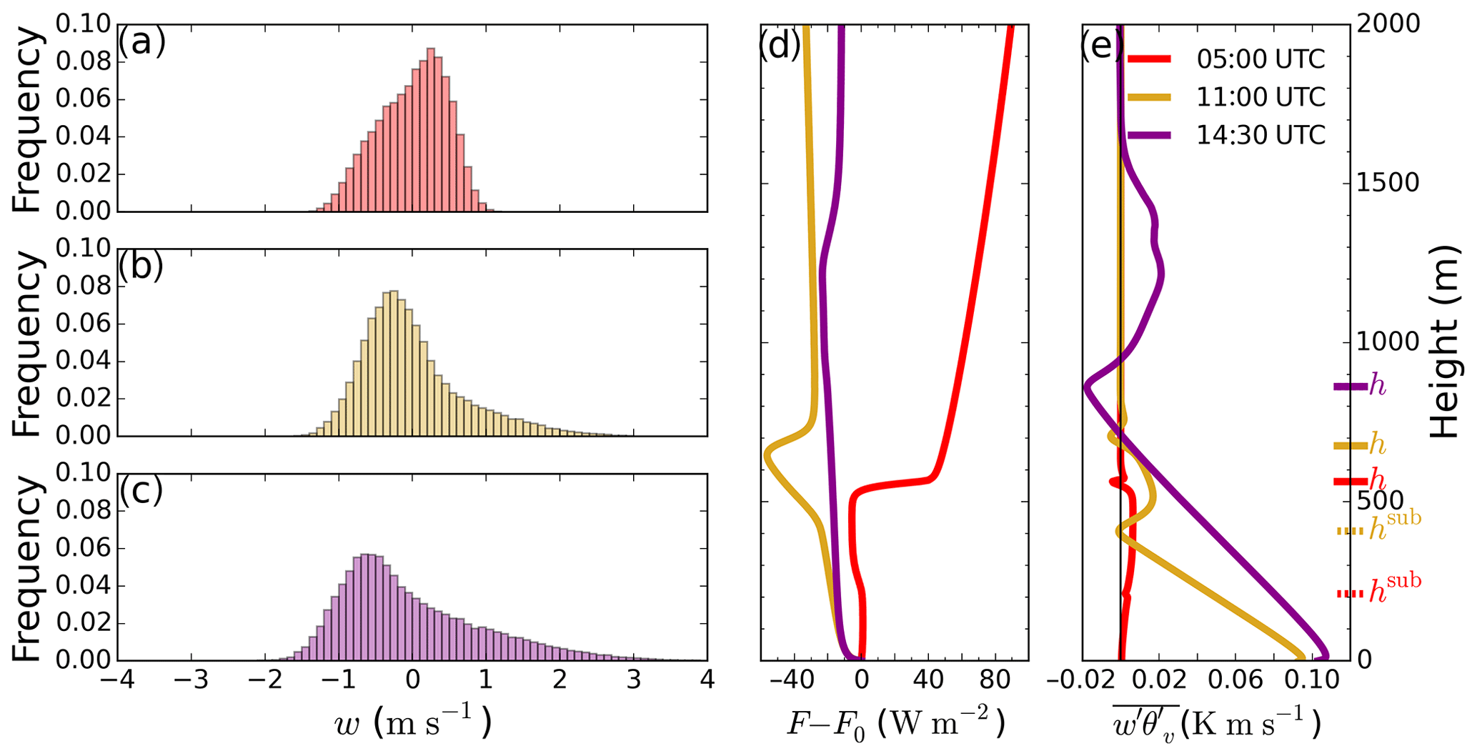
Figure 4On the left, frequency distribution of vertical velocities at at 05:00 UTC (a), 11:00 UTC (b) and 14:30 UTC (c). In the center (d), vertical profile of slab net radiative flux normalized over the surface value at 05:00 UTC (red), 11:00 UTC (dark yellow) and 14:30 UTC (purple). On the right (e) and following the same color code, slab-averaged buoyancy flux . The subcloud layer height hsub and the boundary layer height h are shown for each time at the right vertical axis in (e). At 14:30 UTC both heights coincide.
3.2 Transition on turbulence and radiation
The turbulent spatial structure explaining this transition from typical nocturnal stratocumulus to convective clouds is shown in Fig. 3 through the buoyancy flux and temperature profiles. The initial stages of the LES experiment (Fig. 3a, b, c) present a well-mixed and fully coupled layer from the surface to the cloud top. This layer is limited by a strong jump in liquid water potential temperature θl of about 4 K at 05:00 UTC (Fig. 3a) at around 550 m and a very thin inversion layer. We quantify this layer through its lower and upper limits zi− and zi+, respectively. These heights are defined, following van der Dussen et al. (2016), as the heights above and below, respectively, the maximum in slab-averaged and , at which 5 % of is reached. The thresholds defining zi− and zi+ are set to be constant over the whole simulation for the sake of consistency and easier comparison with previous studies. In Fig. 3b, the liquid water mixing ratio ql shows a linear increase with height within the cloud layer typical of well-mixed stratocumulus clouds (Duynkerke et al., 1995; Wood, 2012). After some hours the boundary layer evolves into a well-mixed subcloud layer with a conditionally unstable cloud layer aloft at 14:30 UTC and a very broad inversion layer. Such evolution of the inversion layer enables us to interpret the typically conditionally unstable region of the cloudy layer in convective conditions as an expanded analogue of the very sharp inversion layer near the top of Sc clouds. Note that this layer includes the sharper inversion layer common in cumulus-topped boundary layers and present in Fig. 3g, h, i between 1200 and 1300 m. Thus, to correctly represent the transition studied here it is necessary to treat the evolution as a transition where the inversion layer expands as the boundary layer grows. A more detailed evolution of the inversion layer is given in Fig. 5. Furthermore, the cloud fraction in the lower part of the cloud layer at 14:30 UTC resembles that of shallow cumulus clouds (Siebesma et al., 2003). In this case, however, a second peak in cloud fraction and larger ql reveals the presence of more clouds at around 1200–1300 m. These clouds are the remnants of the stratocumulus higher part.
In the absence of mechanical production of turbulence, buoyancy is the only driving mechanism for turbulence. Figure 3c, f and i quantify the shift of buoyancy-driven turbulence generation from cloud top radiative cooling at 05:00 UTC to surface warming at 14:30 UTC. Note the change in scale by a factor of 10 in between Fig. 3c and i. Such a difference in magnitude shows that the surface-driven turbulence after sunrise becomes stronger, by about 10 times, than the one created by cloud top cooling. In fact, the cloud top cooling contribution to the buoyancy flux is in part diminished by a compensating condensational warming within the cloud layer. At 11:00 UTC there is a critical moment in the transition: the cloud layer remains rather homogeneous, but the mixed layer is now simultaneously driven both by surface warming and cloud top cooling. As will be shown later (Figs. 4 and 6), the penetration of shortwave radiation through the cloud layer down to the surface is key in regulating both phenomena. The warming of the cloud layer leads to a decoupling of the cloud and subcloud layers. This is already visible at 11:00 UTC with a temperature difference between layers of about 0.2 K at 400 m high (see inset in Fig. 3d).
By resolving interactively the radiation transfer along the cloud layer and the surface response, we gain insight into the dynamical transition, as shown in Fig. 4. There, we observe how the vertical velocity distribution in the middle of the boundary layer starts from a situation with limited extreme velocities (between −1.3 and 1 m s−1) and a negative skewness of at 05:00 UTC, where . This value for Sw lies within the limits of typical marine Sc clouds (Ghate et al., 2014). It then evolves into a prototypical convective boundary layer (CBL) skewed distribution with a larger spread of vertical velocities at 11:00 UTC (between −1.5 and 2.7 m s−1) and Sw=1.2 at half of the boundary layer height, these skewness values being typical of dry convective boundary layers (Lenschow et al., 2012) or situations with cumulus coupled to Sc clouds (de Roode and Duynkerke, 1996). Similar values for Sw are found at 14:30 UTC, with minimum and maximum vertical velocities between −1.8 and 3.5 m s−1, respectively. The transition from stratocumulus to prototypical convective conditions is reinforced by the evolution of the radiative profiles. Figure 4d shows an initial net radiative divergence at the cloud top of 43 W m−2. The related cooling drives the mixed layer at 05:00 UTC. At this time the radiative cooling is stronger than the warming by entrainment as the mixed layer cools at a rate of about 0.1 K h−1 before sunrise (not shown). By 11:00 UTC there is a net radiative warming along the cloud layer (between 400 and 650 m high; see Fig. 3) due to the absorption of shortwave radiation within the cloud layer. Shortwave radiation locally warms up the lower two thirds of the cloud layer to 1.1 K h−1 due to the 44 W m−2 of absorbed shortwave radiation along its travel through the cloud layer (not shown). The high cloud droplet number, 300 cm−3, is likely to influence such net warming positively.
This net radiative warming along the cloud layer reinforces the warming driven by entrainment of free-tropospheric air. The combination of both processes is critical for the decoupling of the cloud and subcloud layers. As will be shown later (Fig. 6), it also plays a role in the thinning of the Sc and the reduction in turbulence generation at the cloud top. Figure 4e shows the profile of the buoyancy flux, closely linked to the role of radiation. The averaged buoyancy flux shows a similar transition starting from prototypical nocturnal Sc clouds at 05:00 UTC, with positive buoyancy along the whole layer up to 550 m and a local minimum at the cloud base due to latent heat release (Bretherton and Wyant, 1997; Wood, 2012). We define the height of such a minimum as the subcloud layer height hsub. The definition of hsub is necessary to better quantify the decoupling of the stratocumulus layer from the surface, as will be shown in Fig. 10. At the cloud top, Fig. 4e presents an absolute minimum at the boundary layer height h at 05:00 UTC. The buoyancy flux profile at 11:00 UTC shows the decoupling of the cloud layer from the surface by the enhancement of the local minimum at hsub at 400 m. This nearly negative value in the vicinity of the cloud base has already been described as an indication of decoupling and hampered transport of moisture (and heat, in our case) from the surface to the cloud layer (Turton and Nicholls, 1987; Stevens, 2000; Lewellen and Lewellen, 2002). This will be further explored in Fig. 10. The buoyancy profile evolves at 14:30 UTC to a profile common in cumulus-topped convective boundary layers (Siebesma et al., 2003) or decoupled Sc cloud layers (Wood, 2012). It shows a linearly decreasing up to the cloud base and buoyantly active convective clouds above 950 m. Note that under such conditions the boundary layer height and the subcloud top height coincide and hsub=h.

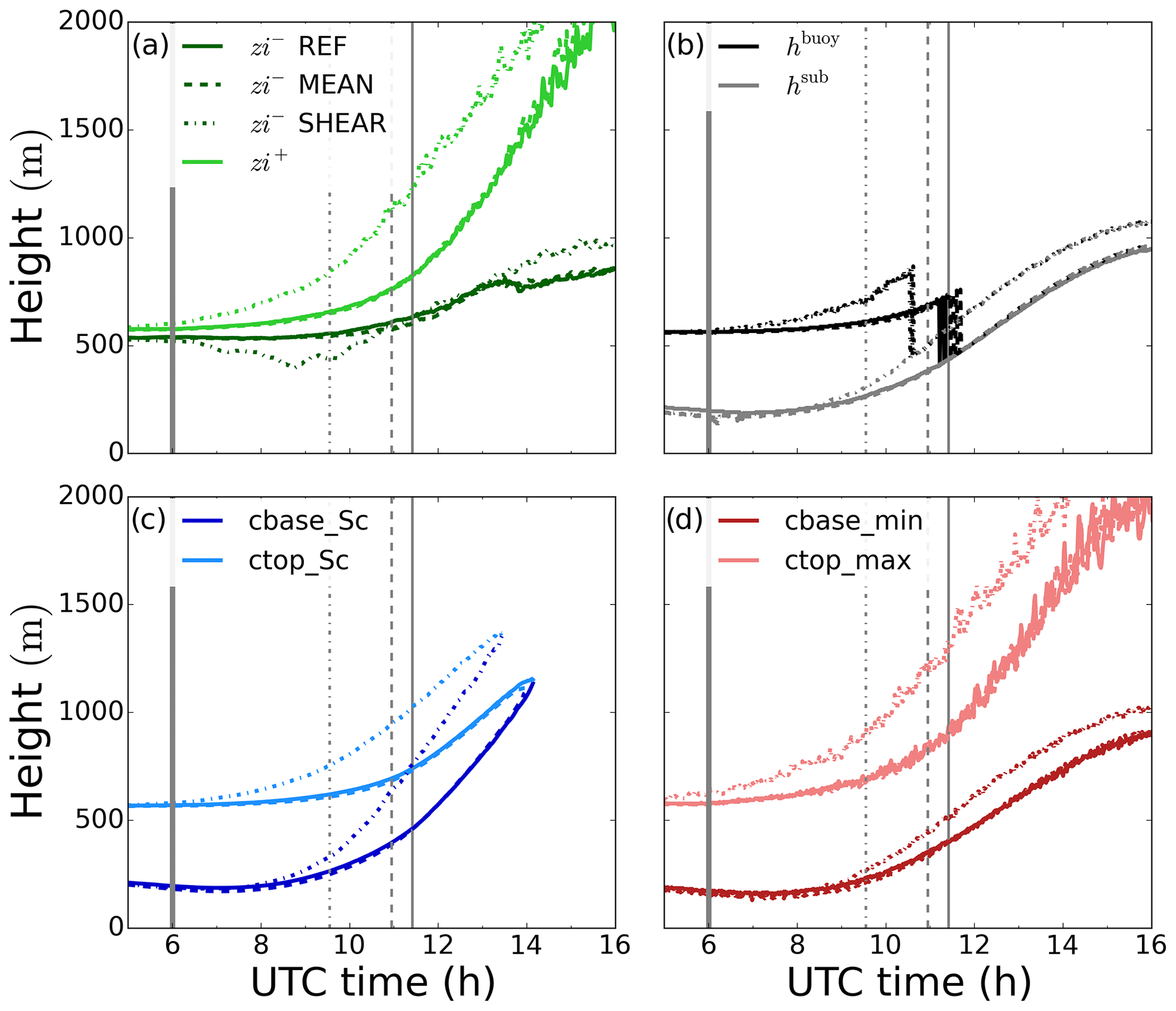
Figure 5Time series of inversion layer top zi+ (light green) and bottom zi− (dark green) heights, boundary layer height h (black) and subcloud buoyancy minimum height hsub (grey), stratocumulus cloud base cbase_Sc (dark blue) and top ctop_Sc (light blue) heights, and minimum cloud base cbase_min (dark red) and maximum cloud top ctop_ max (light red) heights. Sunrise time and cloud breakup time are indicated by the thick and thin grey lines, respectively.
We show in the time series in Fig. 5 the evolution of the variables that better reflect the dynamics of the Sc–Cu transition: we show the inversion layer upper and lower limits zi+ and zi−, respectively, the subcloud top height hsub and boundary layer height h shown in Fig. 4, and the maximum cloud top and minimum cloud base heights as in Fig. 2, and we additionally calculate the Sc cloud base cbase_Sc and cloud top ctop_Sc. These are defined as the height of the lowest and highest vertical level, respectively, with a slab-averaged cloud fraction higher than 40 %. After 10:00 UTC the Sc cloud base rises faster than the minimum cloud base. This is analogous to the slower rise of the Sc cloud top compared to the maximum cloud top. Due to a faster rise of the Sc cloud base than the Sc cloud top, there is a thinning of the Sc layer eventually dissipating at 14:00 UTC. Lohou et al. (2019) observed a similar cloud thinning pattern based solely on observations. The cloud and subcloud layer dynamics divert from coupled Sc conditions, i.e., a well-mixed layer from the surface to the cloud top, several hours before, as was shown in Figs. 3 and 4. Between 11:00 and 11:30 UTC, i.e., before the cloud breakup, h shifts from the cloud top to the subcloud layer top represented by hsub. The evolution of the inversion layer, indicated by zi+ and zi−, reveals a broadening of the inversion layer from a very thin layer (∼50 m) across the cloud top during the first few hours to a region thicker than 1 km in the afternoon due to the cumulus clouds.
3.3 LWP budget before and during the transition
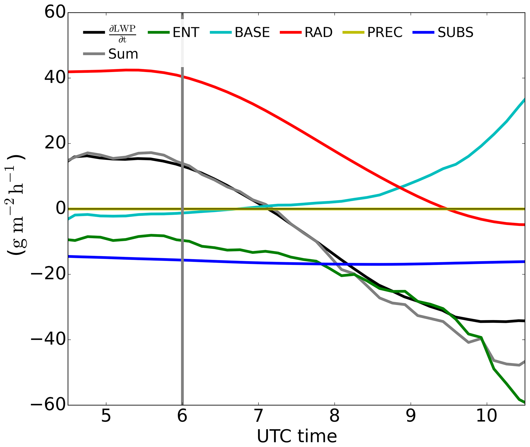
After observing the transition in cloud characteristics and buoyancy regime, a question immediately arises: what is the relative contribution of the main physical processes driving this transition? To this end and relating to Fig. 2b, LWP is calculated and used as the metric to describe the state of the transition and calculate the budget derived by van der Dussen et al. (2014). The budget reads
with
with BASE representing the effect of turbulent fluxes at the cloud base, ENT that of entrainment, PREC the effect of precipitation, RAD that of radiation, and SUBS the one due to subsidence. Δqt and Δθl are the jumps across the inversion layer for total water mixing ratio and liquid water potential temperature, respectively, defined as in van der Dussen et al. (2016): and . δP and δFrad represent the difference in precipitation and net radiation, respectively, between the top of the inversion layer zi+, assumed to be the same as Sc cloud top height in van der Dussen et al. (2016) and the Sc cloud base (van der Dussen et al., 2016). The rest of the variables in Eq. (3) are listed in Appendix A.
In short, this budget enables us to decompose the thinning or thickening of the cloud layer, quantified by a LWP tendency, and relate each contribution to the physical processes governing the stratocumulus clouds. To derive such a budget van der Dussen et al. (2014) assumed the cloud layer to be horizontally homogeneous and vertically well-mixed, implying a linear increase in the liquid water with height within the cloud layer following an adiabatic liquid water profile. The first hours of the simulation perfectly fit those conditions. However, after some hours the horizontal heterogeneities created in the Sc layer and the formation of convective clouds below (see Fig. 5) do not allow these assumptions to hold any longer. Furthermore, the assumption of one well-mixed cloud layer breaks after 10:00 UTC due to the warming by radiation and entrainment (Fig. 4). The distance between zi+ and ctop_Sc, assumed to be negligible by van der Dussen et al. (2014), increases with time up to 50 m at 10:00 UTC. For this reason we focus our analysis on the first stage of the transition until 10:00 UTC.
Before sunrise we observe in a net thickening of the cloud layer Fig. 6 by almost 20 g m−2 h−1, i.e., a growth of about 15 %, driven solely by the longwave cooling at the cloud top (RAD term). During the entire experiment SUBS remains almost constant given the small variation in subsidence with height, showing a negative tendency of around 16 g m−2 h−1. The negative tendency by entrainment (ENT) is to a large extent initially due to the entrainment of warm air (second term in ENT in Eq. 3) since, as shown in Fig. 1, the free-tropospheric air has a similar moisture content to the cloudy air. The thinning tendency of precipitation is small, accounting for up to 4 g m−2 h−1 when the cloud layer is thickest. The small contribution of PREC despite large LWP is explained by the microphysical characteristics of the region. The large cloud condensation nuclei (CCN) concentrations typical for SWA (300 cm−3 in our study) prevent any large effects of precipitation even in Sc with high liquid water content. The effect by cloud base fluxes before sunrise is of a similar magnitude: the turbulent transport of warm air (second term of BASE in Eq. 3) dominates over its moistening effect (first term of BASE in Eq. 3) at this time. Yet the negative net effect by BASE in the LWP tendency is about 10 orders of magnitude smaller than that of RAD.
After sunrise the warming effect of shortwave radiation increasingly offsets the longwave cooling at the cloud top. This leads to a decreasing contribution of RAD to the thickening of the cloud layer. Due to this factor, the sign of the LWP tendency changes at around 07:15 UTC. This is the time when the thinning leading to the eventual cloud breakup starts. Correlated to the shortwave radiation increase after sunrise, the surface-driven growth of the boundary layer leads to larger entrainment rates, thus increasing the warming of the cloud layer through the free-tropospheric engulfed air. An additional factor to the already mentioned warming explains the fast shift to more negative tendencies for the ENT term after 07:00 UTC: the increased drying through entrainment. This drying increases due to two factors enhancing Δqt, from −0.27 g kg−1 at 07:00 UTC to −1 g kg−1 at 10:00 UTC: the moisture input in the boundary layer by the surface and the growth of the boundary layer itself across a drier free troposphere. This larger moisture jump enhances the impact of entrainment by (a) drying the cloud layer and (b) enhancing the entrainment velocity as the difference in buoyancy between the cloud and free troposphere decreases. By the end of this period, at 10:00 UTC, the positive contribution to LWP of cloud base fluxes (BASE) rises to up to 30 g m−2 h−1. This is explained by the increase in surface fluxes (Fig. 2c) and surface buoyancy (Fig. 4e) as the available net radiation at the surface grows. These changes lead to a larger contribution of the moistening term to BASE in Eq. (3), while the warming term including remains less variable for the first hours. Note that although the moisture flux increase at the cloud base implies a growth of LWP in the budget, such moisture growth may eventually contribute to the dissipation of the cloud layer: increased surface moisture flux at the surface and consequently, at the cloud base, relates to enhanced buoyancy through latent heat release and larger turbulence within the cloud layer, known to increase entrainment (Ghonima et al., 2016; Kazil et al., 2016). Such accelerated entrainment leads to the warming of the upper cloud and thus counteracts the mixing of the cloud layer necessary for the maintenance of the Sc.
Comparing the contributions before sunrise in our case to those of the first night in van der Dussen et al. (2016), we find a RAD term almost 30 % lower in our case. Given the similar LWP and θl jump above the cloud top, we attribute the significant difference to the lack of a moisture jump here and thus, weaker cloud top radiative cooling. The BASE term reached values of about 60 g m−2 h−1 in van der Dussen et al. (2016), while we found very little contribution of such a term during the morning due to the compensation of moistening and warming effect of turbulent fluxes. This large difference compared to a marine case shows the relevance of the land surface, as the moistening is limited here and counteracted by a larger warming through turbulent fluxes at the cloud base compared to a marine case. The nighttime ENT term is in our case about 2 to 3 times smaller than in van der Dussen et al. (2016), explained by larger turbulence created by a stronger RAD in their study. All in all, the total tendency is of the same order of magnitude for both cases, although the drivers remain quite different. The increasing negative contribution to the LWP budget by entrainment at daytime is consistent with the Sc-over-land case by Ghonima et al. (2016). We find our case to fall between their cases with fixed Bowen ratios of Bo=0.1 and Bo=1, as we observe nearly Bo=0 during the night growing up to 0.6 during the day in the current case, similar to the measured conditions (Fig. 2c). This indicates the advantage of having a land surface model correctly partitioning the available net energy into surface and latent heat fluxes. In our case, the BASE term behaves similar to their Bo=0.1 case as it also shows a positive contribution to cloud thickening or LWP increase.
3.4 Effect of wind and wind shear in the transition
3.4.1 Nighttime effects
We showed that the transition from stratocumulus to cumulus over land for typical SWA conditions can take place under windless conditions. Given the recurrent presence of wind and low-level jet in the morning during the observational campaign, it is interesting to further investigate the effects that wind has on the transition. Thus, we extend the previous results considering the further effects that mean wind (MEAN) and additional wind shear at the cloud top (SHEAR) have on the transition described. In Table 1, we include the timing and magnitude of the reference metrics for each experiment. Under cloudless conditions, the effect of shear at the surface as well as at the boundary layer top acts as a local source of TKE (Conzemius and Fedorovich, 2006). In our case, such modifications in turbulence may affect the evolution of the cloud transition described in previous sections. First, in Fig. 7 we show the relative differences between the terms defined in Eq. (3) as part of the LWP budget. Following van der Dussen et al. (2016), we show the accumulated difference, starting at 04:30 UTC, of the LWP tendency due to each term between MEAN or SHEAR and the reference simulation REF. Taking the precipitation contribution PREC as an example, we calculate
and similarly for all the other terms present in Eq. (2).
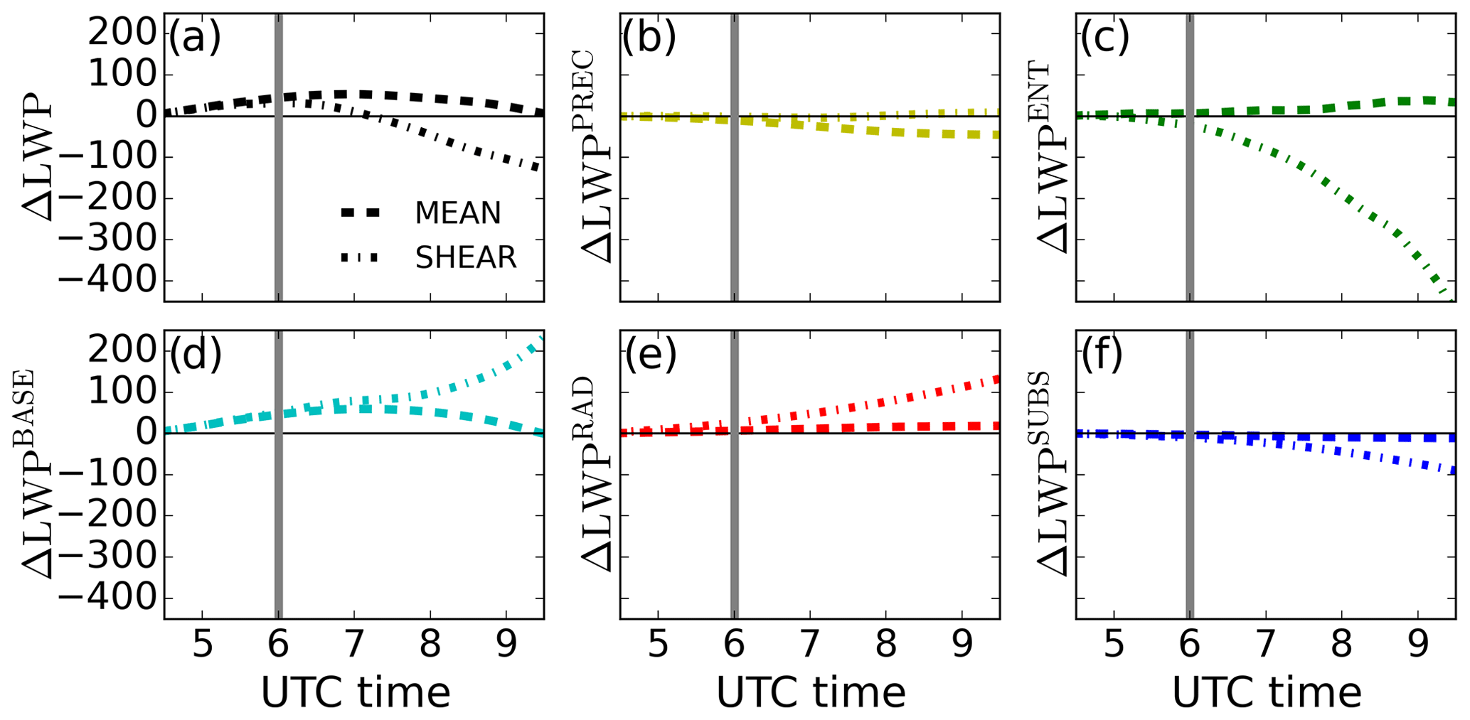
The presence of a light mean wind (3 m s−1) in the entire domain only has minor effects on the first part of the transition: Fig. 7 shows a slightly larger LWP for the MEAN experiment compared to REF. The larger LWP is driven by the increased contribution of the turbulent fluxes at the cloud base (BASE) and particularly the contribution of the moisture flux. For both MEAN and SHEAR experiments, BASE shows a thickening contribution already before sunrise, whereas it was a net thinning contribution in the REF experiment. The change in BASE is explained as follows: wind enhances latent heat flux as well as turbulent generation near the surface, favoring the transport of moisture to the cloud layer. The enhanced turbulence generation near the surface due to the wind, both in MEAN and SHEAR, is visible in the lower part of Fig. 8a. We show there the contributions by the buoyancy and shear terms, B and S, respectively, to the TKE tendency budget and the good agreement regarding surface TKE between our experiments and the observations. Enhanced LWP in nighttime Sc by the presence of wind was also found by Kazil et al. (2016) and attributed to enhanced buoyancy production of TKE due to latent heat release in cloud updrafts. Such findings coincide with the enhanced buoyancy term B for MEAN in Fig. 8a. Precipitation, acting as a negative feedback on LWP, attenuates the effect by BASE in the total tendency of LWP. The remaining terms show little variation between REF and MEAN.
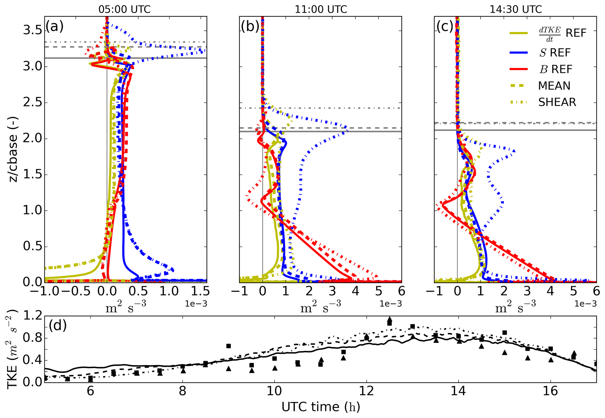
Figure 8Slab-averaged vertical profiles of 20 min averaged turbulent kinetic energy tendency (yellow line), shear contribution (blue line) and buoyancy contribution (red line) for REF (solid line), MEAN (dashed line) and SHEAR (dotted–dashed line) at 05:00 (a), 11:00 (b) and 14:30 UTC (c). The height is normalized by cloud base height at the vertical axis. Following the same line coding, grey horizontal lines indicate the cloud top for each time and experiment. In (d) and following the same line coding are the time series of the simulated turbulent kinetic energy at 10 m high and, indicated by triangles and squares, as observed by two independent stations at the Savè supersite on 26 June 2016.
Wind shear at the top of the cloud layer introduces larger changes: it is known to enhance TKE locally but with a total negative effect on cloud TKE due to reduced buoyancy production (Wang et al., 2012), and it is also known to enhance entrainment at the cloud top (Mellado, 2017). Before sunrise, cloud layer LWP as well as cloud base and cloud top heights (Fig. 9d) show small differences between the SHEAR and MEAN experiments. SHEAR shows systematically lower LWP (not shown) but a thicker Sc cloud layer, e.g., ≃40 m thicker before sunrise, due to increased entrainment velocities. Similarly, we also find a turbulent and clear sublayer between the cloud top and the inversion layer top in SHEAR (Fig. 9a). These results agree with the findings by Wang et al. (2008) and McMichael et al. (2019), who studied cloud top shear effects on marine Sc clouds. Such agreement reinforces the analogy between the nocturnal Sc cloud studied here before sunrise and the typical marine Sc, given the low values of the surface fluxes.
Although they have similar tendencies in the LWP budget before sunrise, the sources for turbulence and, thus, mixing within the cloudy layer are different in MEAN and REF compared to SHEAR. As shown in Fig. 8a, SHEAR shows a much larger contribution by wind shear S to the TKE tendency at the cloud top: up to 1.5 m2 s−3 or more than 5 times the local buoyancy contribution B within the cloud layer. SHEAR also exhibits a slightly lower contribution by buoyancy from cloud top to surface. The larger contribution by S is a consequence of the varying wind speed in the cloud boundary, while the cause for lower B throughout the whole layer lies in the weaker cooling at the cloud top (not shown) due to the shear-induced broader inversion layer (Mellado, 2017): the inversion layer is more than 80 m thick before sunrise at SHEAR, while it is about 40 m in REF and MEAN (see Fig. 9a). The increase in the depth of this layer results in a decrease in the longwave cooling at the cloud top (from about −6.1 K h−1 in MEAN or REF to −4 K h−1 in SHEAR) as the gradients are smoothened and the time air is exposed to the cooling is decreased (Yamaguchi and Randall, 2008). Wang et al. (2008, 2012) also found weaker cooling at the cloud top and a thicker inversion layer on sheared Sc.
The little differences between MEAN and REF at cloud top turbulent properties in terms of S and B (Fig. 8a) reinforce the idea that the turbulence generated by wind shear at the surface in MEAN needs to be transported up to the top of the well-mixed layer to affect entrainment and the overall dynamics of the boundary layer. Yet the traveling turbulence is subject along its rise from the surface to the cloud top to the turbulent cascade, partly dissipating and having a reduced impact on the entrainment zone (Conzemius and Fedorovich, 2006). By contrast, local shear at the cloud top in SHEAR locally generates turbulence to immediately affect entrainment and boundary layer growth. We show in the coming section that the presence of shear at the cloud top after sunrise promotes a faster breakup of the cloud layer.
3.4.2 Daytime effects
After sunrise the shear effects drive the cloud layer towards lower LWP due to enhanced entrainment of warm air (Fig. 7c). The enhanced entrainment velocity in SHEAR is more visible (h growth as a proxy for we in Fig. 9b) after the decoupling of the cloud layer and surface between 09:00 and 10:00 UTC (see Table 1). We attribute the increase in we not only to the presence of local shear at the cloud top but also to the positive feedback between surface fluxes and cloud thinning (Ghonima et al., 2016), further reinforced by wind shear in this case: the slightly lower LWP after sunrise in SHEAR enhances the turbulent fluxes both at the surface (Fig. 8b, c) and cloud base (Fig. 7d). Larger daytime turbulence within the cloud layer leads to a thicker slab average inversion layer. However, the presence of shear and enhanced turbulence near cloud top leads to a wavier and more irregular inversion layer. As a result, there is a local thinning of the inversion layer, allowing for a locally enhanced wind shear (Mellado, 2017) and, thus, further entrainment, which will lead to a more negative rate for and the subsequent increase in surface fluxes. Furthermore, the accelerated growth of the boundary layer in SHEAR leads to a larger moisture difference between the cloud layer and the air above, thus further reinforcing the negative effects of entrainment through additional drying in ENT (Fig. 7) in the tendency of cloud layer LWP.
On the other hand, radiative cooling (RAD) remains a positive contribution for for a longer time (see Fig. 7e). The reason is the thicker integration layer, caused by wind shear, over which RAD is evaluated. This layer ranges from cbase_Sc to the inversion layer top (zi+) for the budget in Eqs. (2) and (3). As assumed by van der Dussen et al. (2016), zi+ and ctop_Sc agree quite well for thin inversion layers such as the one during the night without shear in REF (see Fig. 5) and the choice is unimportant. The agreement worsens when shear is present, as the inversion layer thickens and ctop_Sc and zi+ show larger discrepancies (Fig. 9), as also shown by Wang et al. (2012). This thicker layer over which RAD is calculated explains the larger divergence in the net radiative flux between the cloud base and zi−. Thus, a sensitive point for the discussion is the definition of the limits: one may wonder if the larger contribution to LWP gain of RAD in SHEAR may be an artifact of the boundaries selected for the budget in Eq. (2). Using other limits at the top, such as ctop_ Sc or cloud top, however, lead to a worse closure of the budget.
The negative LWP tendency is hampered in SHEAR by the positive contribution of BASE (Fig. 7d). The increase in BASE is explained as part of the positive feedback stated above: given the lower LWP at sunrise more shortwave radiation reaches the surface, increasing the surface fluxes, specially, the latent heat flux. Thus, we deduce that the initial lower LWP in SHEAR accelerates the further thinning and eventual breakup of the cloud layer due to two factors enhancing entrainment: the direct enhancement due to local shear at the cloud top and the indirect one due to larger surface fluxes and boundary layer growth. This is represented in the LWP budget by more negative and positive values for ENT and BASE, respectively.
Figure 9 completes the analysis of wind sensitivity after the decoupling of the cloud layer. In agreement with the previous explanation, MEAN evolves similarly to REF as the wind-driven increase in surface fluxes is negligible compared to the boundary layer dynamics. Larger entrainment velocities accelerate the growth of the boundary layer in SHEAR, as well as the rise of the cloud top and cloud base of both the total and Sc cloud layers (Fig. 9c, d). The faster growth of the boundary layer with shear at its top is a well-documented feature (Conzemius and Fedorovich, 2006; Liu et al., 2018). The faster-rising cloud layer in SHEAR coincides with an earlier negative buoyancy flux minimum at the cloud base and, thus, an earlier decoupling of the cloud layer by almost 2 h (Table 1). Besides the shear effects, the larger surface fluxes due to a lower LWP after sunrise also explain the faster growth of the subcloud layer buoyancy flux minimum. Similarly, the inversion layer grows faster in SHEAR due to both a decreasing zi− and a growing zi+. Following the accelerated processes in SHEAR, the breakup of the cloud layer takes place about 2 h earlier than in REF.
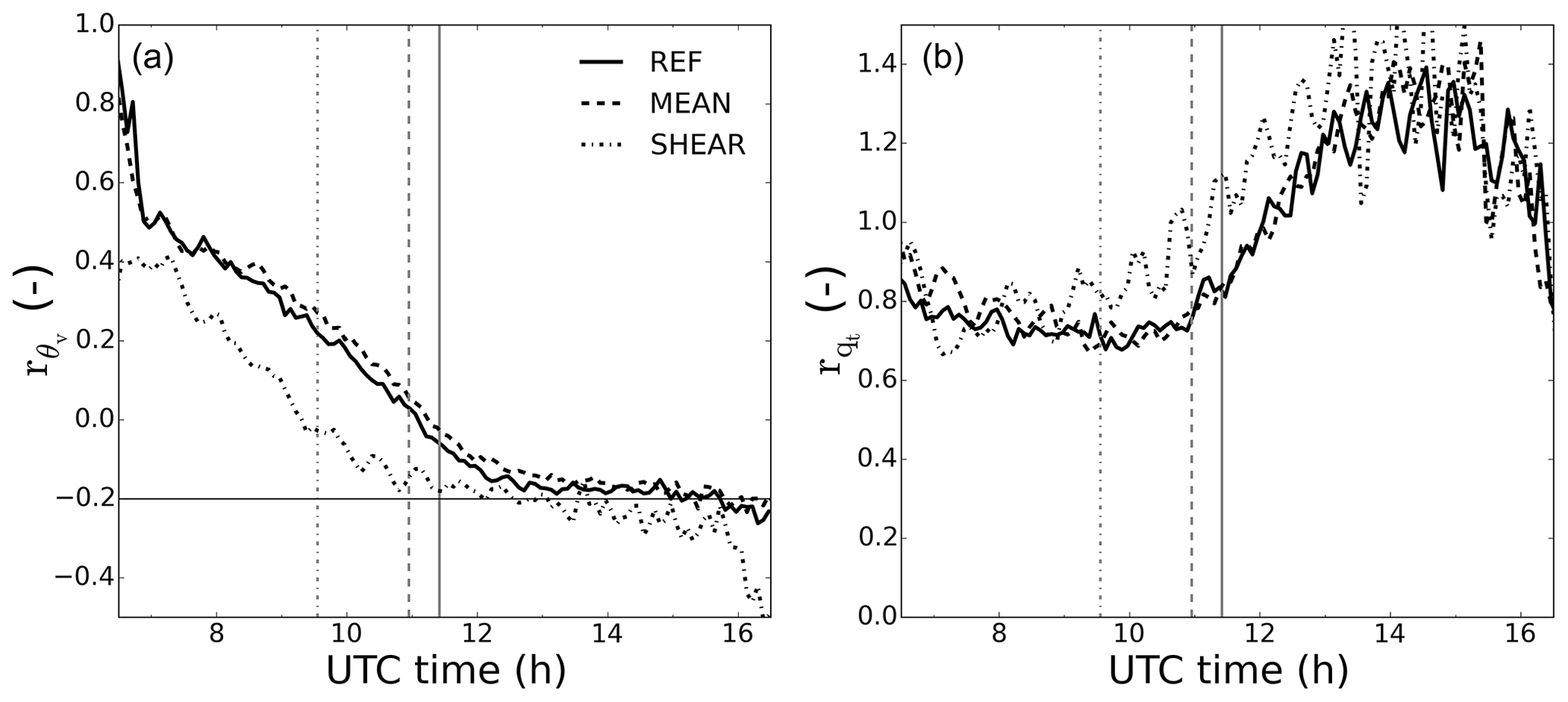
Figure 10Time series of subcloud layer top to surface buoyancy flux (a) and total moisture flux (b) ratio for REF (solid lines), MEAN (dashed) and SHEAR (dotted–dashed). Vertical lines represent cloud breakup for each experiment.
3.5 Representation by large-scale metrics
A transition from stratocumulus to shallow cumulus represented as a continuum and over a period spanning several hours, such as the one shown here, poses challenges to coarser-resolution models in correctly representing cloud fraction, inversion layer height or thickness as well as buoyancy source(s). To quantify the transition and explain its possible drivers beyond 10:00 UTC we calculate two metrics traditionally used in larger-scale models: the ratio between subcloud layer top buoyancy flux, i.e., the buoyancy flux evaluated at hsub, and surface buoyancy flux and its analogues for the total moisture flux in Fig. 10. is frequently used to parameterize entrainment velocities at the boundary layer top, while provides information on the transport of moisture from the surface to the cloud and subcloud layer. These two metrics show the impact of the surface fluxes, in terms of buoyancy and moisture, on the boundary layer and capture the dynamics of it.
shows a linearly decreasing trend, showing the lowering transport of buoyancy to the cloud layer as the cloud-top-driven circulation weakens; the surface buoyancy flux grows and so does the slope of the linearly decreasing vertical buoyancy flux. Around 11:00 UTC the sign of reverses (see also the nearly negative buoyancy flux minimum at hsub in Fig. 4d). This explicitly indicates the decoupling between the cloud layer and the surface. After 12:00 UTC approaches the typical ratio of −0.2 for dry CBLs (Stull, 1988) until the decay of turbulence generation at the surface by the end of the experiment. Similarly, presents slightly decreasing values from 0.8 to 0.7 after sunrise. This was also found in other studies of marine Sc by de Roode et al. (2016), who mentioned that implies a net moistening of the subcloud layer. As shown in Fig. 6, the moistening and warming of the cloud layer by turbulent fluxes from the surface almost offset each other in terms of LWP impact for the first hours after sunrise. After the shift in h and before the breakup at 11:30 UTC we observe growing values for representing a weaker moistening of the subcloud layer. After 12:00 UTC we find values higher than 1, indicating a net drying of the subcloud layer and consequent moistening of the cloud layer by surface evapotranspiration. MEAN shows little variation from REF, reinforcing the small effect of the mean wind in the transition. The only remarkable difference is a 1 h delay in reaching values of near a typical CBL of −0.2, due to the fact that under convective conditions, mean wind may hamper the turbulent updrafts from the surface to the boundary layer top, thus reducing the related entrainment (Liu et al., 2018). SHEAR shows a qualitatively similar pattern to REF after sunrise with an earlier shift in the sign of of about 2 h. Afterwards, reaches values lower than −0.2 in SHEAR. This suggests that as found by Conzemius and Fedorovich (2006), the buoyancy entrainment flux is enhanced compared to clear CBLs.
Table 1Values and time of the main features in the stratocumulus-to-cumulus transition for the three experiments REF, MEAN and SHEAR.

Based on observations of the DACCIWA project in southern West Africa we designed a numerical experiment to reproduce the transition from nighttime stratocumulus to daytime cumulus clouds over land. Special emphasis is placed on the stratocumulus deck breakup and the role of the surface and boundary layer processes. This was done by means of a large eddy simulation with an interactive radiation scheme and a plant-mechanistic land surface model, allowing for coupled responses of radiative profiles and surface fluxes to changes in the thermodynamic fields and surface conditions. Numerical experiments were evaluated against a complete set of observations.
We quantified the transition in terms of inversion layer height and thickness, cloud top and cloud base heights, and boundary layer height. These metrics remain largely constant over time during the night and similar to typical marine stratocumulus clouds and start to diverge from these values a few hours after sunrise. The main drivers are the increased entrainment due to the enhanced turbulence driven by the surface fluxes and, to a lesser extent, the shortwave radiative warming at the cloud top. We further showed how temperature, vertical velocity distributions, and buoyancy and radiative fluxes vary during the transition period. Notable features during the transitions are the decoupling of the cloud layer by 11:00 UTC supported by (1) two independent well-mixed layers seen in the temperature profiles and (2) a negative subcloud buoyancy flux minimum. The radiative fluxes shift from exerting a net cooling effect to a warming within the cloud layer which, in addition to the warming by entrainment, leads to the mentioned decoupling.
We further described and quantified the varied physical processes that maintain and thin the stratocumulus cloud layer using the LWP budget (van der Dussen et al., 2016). The radiative term is the most dominant process contributing to LWP increase during nighttime, while its contribution decreases after sunrise and becomes a sink of LWP due to increasing shortwave radiation warming. Subsidence has a negative and fairly constant contribution to the budget during the whole transition. Precipitation and cloud base fluxes, the latter driven by the cloud top cooling circulation, have almost no effects during the night. As the day progresses, the moisture flux from the surface contributes increasingly to the growth of LWP. Entrainment has a negative and nearly constant contribution during the night. After sunrise, the entrainment-induced LWP thinning intensifies due to cloud layer rise and the increasing moisture difference between the cloud layer and the air above.
Lastly we investigated the effect of wind on the transition. Two additional experiments were performed along with the windless reference experiment: one experiment with a mean wind of 3 m s−1 at all heights and another with an additional wind jump at the cloud top of 5 m s−1 and further increase of 5 m s−1 km−1 above. The geostrophic wind was assumed to be identical to the prescribed wind in each experiment. The aim was to represent the main features of a recurrent low-level jet observed in the region during the nighttime and morning. We found the mean wind to have almost no impact on the transition. However, the shear at the cloud top had larger effects. Before sunrise, the inversion layer was thicker and the TKE generation by shear was higher at the cloud top at the expense of lower generation by buoyancy. These features are typical of sheared marine Sc. After sunrise, shear accelerated cloud thinning, boundary layer growth and the transition to a convective boundary layer. This was due to the direct effect of shear on entrainment growth similar to clear convective boundary layers, but also to the enhanced surface fluxes as the cloud layer thinned faster. The related enhanced entrainment contributed to a faster thinning of the cloud layer, leading to a breakup 2 h earlier than in the no-wind experiment.
We calculated widely used ratios that characterize the prototypical clear and cloudy boundary layer to determine their ability in reproducing the transition. We find that the ratio between the subcloud layer entrainment and the surface turbulent buoyancy fluxes decreases linearly with time during the transition, starting from initial values of and reaching typical dry convective values of −0.2 about 1 h after the Sc deck breakup at about 12:30 UTC. The analogous moisture ratio shows a slight decrease from 0.8 to 0.7 until the shift in buoyancy flux minimum. After the shift, increases reaching values above 1, thus moistening the cloud layer. Mean wind leaves the transition representation by and unaffected, except for a 1 h delay in reaching CBL values for . In contrast, the presence of cloud top shear accelerates the evolution of both and by 2 h. Furthermore, reaches values lower than −0.2 after breakup. These findings reveal the relevance of the land–atmosphere feedbacks on the stratocumulus thinning and cloud transition and the impact of wind on it.
| Variable | Name | Units |
| B | Buoyancy term in TKE tendency equation | m2 s−3 |
| Bo | Bowen ratio | (–) |
| cc | Cloud cover | (–) |
| cfra | Cloud fraction | (–) |
| cp | Dry air specific heat | J kga K−1 |
| cbase_Sc | Stratocumulus cloud base height | m |
| ctop_Sc | Stratocumulus cloud top height | m |
| D | Cloud layer depth | m |
| F | Net radiative flux | W m−2 |
| F0 | Net radiative flux at surface | W m−2 |
| g | Gravitational acceleration | m s−2 |
| h | Boundary layer height | m |
| hsub | Subcloud layer height | m |
| LE | Latent heat flux | W m−2 |
| LWP | Liquid water path | gw m−2 |
| ql | Liquid water mixing ratio | gw kg |
| qs | Saturation specific humidity | gw kg |
| qt | Total water mixing ratio | gw kg |
| Rd | Dry air gas constant | J kga K−1 |
| Rnet | Net radiation at surface | W m−2 |
| rϕ | Subcloud to surface ratio | (–) |
| S | Shear term in TKE tendency equation | m2 s−3 |
| SH | Sensible heat flux | W m−2 |
| Sw | Skewness | (–) |
| T | Temperature | K |
| U | Horizontal wind speed | m s−1 |
| we | Entrainment velocity | m s−1 |
| wsubs | Subsidence | m s−1 |
| Turbulent flux of Φ | m s−1 [Φ] | |
| Turbulent flux of Φ at cloud base | m s−1 [Φ] | |
| zi+ | Inversion layer top height | m |
| zi− | Inversion layer bottom height | m |
| γ | gw kg K−1 | |
| gw | ||
| δFrad | Difference in net radiation between zi+ and cbase_Scu | W m−2 |
| δP | Difference in precipitation between zi+ and cbase_Scu | gw g m s−1 |
| Δqt | qt jump along inversion layer | gw kg |
| Δθl | θl jump along inversion layer | K |
| η | Thermodynamic factor (see van der Dussen et al., 2014) | (–) |
| θ | Potential temperature | K |
| θl | Liquid water potential temperature | K |
| θv | Virtual potential temperature | K |
| Π | Exner function | (–) |
| ρ | Air density | kga m−3 |
The data obtained during the DACCIWA campaign at the Savè supersite are available on the SEDOO database (http://baobab.sedoo.fr/DACCIWA/, last access: 2 March 2020; https://doi.org/10.6096/dacciwa.1618., Derrien et al., 2016; https://doi.org/10.6096/dacciwa.1686, Handwerker et al., 2016; https://doi.org/10.6096/dacciwa.1690, Kohler et al., 2016). The DALES code is maintained and developed by Dutch research centres, mainly Wageningen University, Delft University of Technology and KNMI, and is freely available for download at https://github.com/dalesteam/dales (Wageningen University et al., 2020).
XPB wrote the paper with contributions from all co-authors. XPB carried out the analysis and produced the figures with contributions from BA, KB, CD, NK, FL and ML. JV and SdR contributed to setting up the case on LES. BA, KB, CD, NK, FL, ML, SdR and JV contributed to the analysis of the results. BA, CD, NK, FL, ML and XPB conducted the ground measurements.
The authors declare that they have no conflict of interest.
This article is part of the special issue “Results of the project “Dynamics-aerosol-chemistry-cloud interactions in West Africa” (DACCIWA) (ACP/AMT inter-journal SI)”. It is not associated with a conference.
The authors would like to thank all people whose work was involved in the measurement campaign of DACCIWA and in particular all the people who contributed to the Savè supersite. The first author acknowledges Maurin Zouzua for providing the cloud cover observations, Anna-Lena Deppenmeier for providing ERA-interim data and Shantonu Abe Chatterjee for the useful tips during the writing process. The numerical simulations were performed with the supercomputer facilities at SURFsara and financially sponsored by the Netherlands Organisation for Scientific Research (NWO) Physical Science Division (project number SH-312-15). We would also like to thank two anonymous reviewers for their helpful comments during the review process.
This research has been supported by the NWO (NWOALW Open Programme (grant no. 824.15.013)) and the European Commission, Seventh Framework Programme (DACCIWA (grant no. 603502)).
This paper was edited by Susan van den Heever and reviewed by two anonymous referees.
Ackerman, A. S., Kirkpatrick, M. P., Stevens, D. E., and Toon, O. B.: The impact of humidity above stratiform clouds on indirect aerosol climate forcing, Nature, 432, 1014–1017, https://doi.org/10.1038/nature03174, 2004. a
Adler, B., Babić, K., Kalthoff, N., Lohou, F., Lothon, M., Dione, C., Pedruzo-Bagazgoitia, X., and Andersen, H.: Nocturnal low-level clouds in the atmospheric boundary layer over southern West Africa: an observation-based analysis of conditions and processes, Atmos. Chem. Phys., 19, 663–681, https://doi.org/10.5194/acp-19-663-2019, 2019. a, b, c, d, e, f, g, h
Babić, K., Adler, B., Kalthoff, N., Andersen, H., Dione, C., Lohou, F., Lothon, M., and Pedruzo-Bagazgoitia, X.: The observed diurnal cycle of low-level stratus clouds over southern West Africa: a case study, Atmos. Chem. Phys., 19, 1281–1299, https://doi.org/10.5194/acp-19-1281-2019, 2019. a, b, c, d, e, f
Bauer-Pfundstein, M. R. and Goersdorf, U.: Target separation and classification using cloud radar Doppler-spectra, in: Proceedings of the 33rd Intern. Conf. on Radar Meteorology, Vol. 11.B2, 1–8, Cairns, Australia, available at: https://ams.confex.com/ams/33Radar/techprogram/paper_123456.htm (last access: 2 March 2020), 2007. a
Bellon, G. and Stevens, B.: Using the Sensitivity of Large-Eddy Simulations to Evaluate Atmospheric Boundary Layer Models, J. Atmos. Sci., 69, 1582–1601, https://doi.org/10.1175/JAS-D-11-0160.1, 2012. a
Bessardon, G., Brooks, B., Abiye, O., Adler, B., Ajao, A., Ajileye, O., Altstätter, B., Amekudzi, L. K., Aryee, J. N. A., Atiah, W., Ayoola, M., Babic, K., Bärfuss, K., Bezombes, Y., Bret, G., Brilouet, P.-E., Cayle-Aethelhard, F., Danuor, S., Delon, C., Derrien, S., Dione, C., Durand, P., Fosu-Amankwah, K., Gabella, O., Groves, J., Handwerker, J., Kalthoff, N., Kohler, M., Kunka, N., Jambert, C., Jegede, G., Lampert, A., Leclercq, J., Lohou, F., Lothon, M., Medina, P., Pätzold, F., Pedruzo-Bagazgoitia, X., Reinares, I., Sharpe, S., Smith, V., Sunmonu, L. A., Tan, N., and Wieser, A.: A new high-quality dataset of the diurnal cycle of the southern West African atmospheric boundary layer during the Monsoon season – an overview from the DACCIWA campaign, in preparation, 2020. a
Blossey, P. N., Bretherton, C. S., Zhang, M., Cheng, A., Endo, S., Heus, T., Liu, Y., Lock, A. P., de Roode, S. R., and Xu, K.-M.: Marine low cloud sensitivity to an idealized climate change: The CGILS LES intercomparison, J. Adv. Model. Earth Sy., 5, 234–258, https://doi.org/10.1002/jame.20025, 2013. a
Boucher, O., Randall, D., Artaxo, P., Bretherton, C., Feingold, G., Forster, P., Kerminen, V.-M., Kondo, Y., Liao, H., Lohmann, U., Rasch, P., Satheesh, S. K., Sherwood, S., Stevens, B., and Zhang, X. Y.: Clouds and Aerosols. In: Climate Change 2013: The Physical Science Basis. Contribution of Working Group I to the Fifth Assessment Report of the Intergovernmental Panel on Climate Change, edited by: Stocker, T. F., Qin, D., Plattner, G.-K., Tignor, M., Allen, S. K., Boschung, J., Nauels, A., Xia, Y., Bex, V., and Midgley, P. M., Cambridge University Press, Cambridge, UK and New York, NY, USA, 2013. a
Bretherton, C. S. and Wyant, M. C.: Moisture Transport, Lower-Tropospheric Stability, and Decoupling of Cloud-Topped Boundary Layers, J. Atmos. Sci., 54, 148–167, https://doi.org/10.1175/1520-0469(1997)054<0148:MTLTSA>2.0.CO;2, 1997. a
Bretherton, C. S., Krueger, S. K., Wyant, M. C., Bechtold, P., Van Meijgaard, E., Stevens, B., and Teixeira, J.: A GCSS Boundary-Layer Cloud Model Intercomparison Study Of The First Astex Lagrangian Experiment, Bound.-Lay. Meteorol., 93, 341–380, https://doi.org/10.1023/A:1002005429969, 1999a. a
Bretherton, C. S., Macvean, M. K., Bechtold, P., Chlond, A., Cotton, W. R., Cuxart, J., Cuijpers, H., Mhairoutdinov, M., Kosovic, B., Lewellen, D., Moeng, C.-H., Siebesma, P., Stevens, B., Stevens, D. E., Sykes, I., and Wyant, M. C.: An intercomparison of radiatively driven entrainment and turbulence in a smoke cloud, as simulated by different numerical models, Q. J. Roy. Meteor. Soc., 125, 391–423, https://doi.org/10.1002/qj.49712555402, 1999b. a
Bretherton, C. S., Blossey, P. N., and Uchida, J.: Cloud droplet sedimentation, entrainment efficiency, and subtropical stratocumulus albedo, Geophys. Res. Lett., 34, L03813, https://doi.org/10.1029/2006GL027648, 2007. a
Chen, T., Rossow, W. B., and Zhang, Y.: Radiative Effects of Cloud-Type Variations, J. Climate, 13, 264–286, https://doi.org/10.1175/1520-0442(2000)013<0264:REOCTV>2.0.CO;2, 2000. a
Conzemius, R. J. and Fedorovich, E.: Dynamics of Sheared Convective Boundary Layer Entrainment. Part I: Methodological Background and Large-Eddy Simulations, J. Atmos. Sci., 63, 1151–1178, https://doi.org/10.1175/JAS3691.1, 2006. a, b, c, d
Dearden, C., Hill, A., Coe, H., and Choularton, T.: The role of droplet sedimentation in the evolution of low-level clouds over southern West Africa, Atmos. Chem. Phys., 18, 14253–14269, https://doi.org/10.5194/acp-18-14253-2018, 2018. a
Deardorff, J. W.: Stratocumulus-capped mixed layers derived from a three-dimensional model, Bound.-Lay. Meteorol., 18, 495–527, https://doi.org/10.1007/BF00119502, 1980. a
de Roode, S. R. and Duynkerke, P. G.: Dynamics of cumulus rising into stratocumulus as observed during the first “Lagrangian” experiment of ASTEX, Q. J. Roy. Meteor. Soc., 122, 1597–1623, https://doi.org/10.1002/qj.49712253507, 1996. a
de Roode, S. R., Sandu, I., van der Dussen, J. J., Ackerman, A. S., Blossey, P., Jarecka, D., Lock, A., Siebesma, A. P., and Stevens, B.: Large-Eddy Simulations of EUCLIPSE–GASS Lagrangian Stratocumulus-to-Cumulus Transitions: Mean State, Turbulence, and Decoupling, J. Atmos. Sci., 73, 2485–2508, https://doi.org/10.1175/JAS-D-15-0215.1, 2016. a, b, c
Derrien, S., Bezombes, Y., Bret, G., Gabella, O., Jarnot, C., Medina, P., Piques, E., Delon, C., Dione, C., Campistron, B., Durand, P., Jambert, C., Lohou, F., Lothon, M., Pacifico, F., and Meyerfeld, Y.: DACCIWA field campaign, Savè super-site, UPS instrumentation, SEDOO OMP, https://doi.org/10.6096/dacciwa.1618, 2016. a, b
Dione, C., Lohou, F., Lothon, M., Adler, B., Babić, K., Kalthoff, N., Pedruzo-Bagazgoitia, X., Bezombes, Y., and Gabella, O.: Low-level stratiform clouds and dynamical features observed within the southern West African monsoon, Atmos. Chem. Phys., 19, 8979–8997, https://doi.org/10.5194/acp-19-8979-2019, 2019. a, b, c, d, e, f
Duynkerke, P. G., Zhang, H. Q., and Jonker, P. J.: Microphysical and Turbulent Structure of Nocturnal Stratocumulus as Observed during ASTEX, J. Atmos. Sci., 52, 2763–2777, https://doi.org/10.1175/1520-0469(1995)052<2763:MATSON>2.0.CO;2, 1995. a
Duynkerke, P. G., de Roode, S. R., van Zanten, M. C., Calvo, J., Cuxart, J., Cheinet, S., Chlond, A., Grenier, H., Jonker, P. J., Köhler, M., Lenderink, G., Lewellen, D., Lappen, C.-l., Lock, A. P., Moeng, C.-h., Müller, F., Olmeda, D., Piriou, J.-m., Sánchez, E., and Sednev, I.: Observations and numerical simulations of the diurnal cycle of the EUROCS stratocumulus case, Q. J. Roy. Meteor. Soc., 130, 3269–3296, https://doi.org/10.1256/qj.03.139, 2004. a
Eastman, R. and Warren, S. G.: Diurnal Cycles of Cumulus, Cumulonimbus, Stratus, Stratocumulus, and Fog from Surface Observations over Land and Ocean, J. Climate, 27, 2386–2404, https://doi.org/10.1175/JCLI-D-13-00352.1, 2014. a
Eastman, R., Warren, S. G., and Hahn, C. J.: Climatic atlas of cloudsover land and ocean, available at: https://atmos.washington.edu/CloudMap/ (last access: 2 March 2020), 2014. a
Flamant, C., Knippertz, P., Fink, A. H., Akpo, A., Brooks, B., Chiu, C. J., Coe, H., Danuor, S., Evans, M., Jegede, O., Kalthoff, N., Konaré, A., Liousse, C., Lohou, F., Mari, C., Schlager, H., Schwarzenboeck, A., Adler, B., Amekudzi, L., Aryee, J., Ayoola, M., Batenburg, A. M., Bessardon, G., Borrmann, S., Brito, J., Bower, K., Burnet, F., Catoire, V., Colomb, A., Denjean, C., Fosu-Amankwah, K., Hill, P. G., Lee, J., Lothon, M., Maranan, M., Marsham, J., Meynadier, R., Ngamini, J.-B., Rosenberg, P., Sauer, D., Smith, V., Stratmann, G., Taylor, J. W., Voigt, C., and Yoboué, V.: The Dynamics–Aerosol–Chemistry–Cloud Interactions in West Africa Field Campaign: Overview and Research Highlights, B Am. Meteorol. Soc., 99, 83–104, https://doi.org/10.1175/BAMS-D-16-0256.1, 2018. a
Ghate, V. P., Albrecht, B. A., Miller, M. A., Brewer, A., and Fairall, C. W.: Turbulence and Radiation in Stratocumulus-Topped Marine Boundary Layers: A Case Study from VOCALS-REx, J. Appl. Meteorol. Clim., 53, 117–135, https://doi.org/10.1175/JAMC-D-12-0225.1, 2014. a
Ghonima, M. S., Heus, T., Norris, J. R., and Kleissl, J.: Factors Controlling Stratocumulus Cloud Lifetime over Coastal Land, J. Atmos. Sci., 73, 2961–2983, https://doi.org/10.1175/JAS-D-15-0228.1, 2016. a, b, c, d, e
Gronemeier, T., Kanani-Sühring, F., and Raasch, S.: Do Shallow Cumulus Clouds have the Potential to Trigger Secondary Circulations Via Shading?, Bound.-Lay. Meteorolo., 162, 143–169, https://doi.org/10.1007/s10546-016-0180-7, 2016. a
Handwerker, J., Scheer, S., and Gamer, T.: DACCIWA field campaign, Savè super-site, Cloud and precipitation, SEDOO OMP, https://doi.org/10.6096/dacciwa.1686, 2016. a, b, c
Hannak, L., Knippertz, P., Fink, A. H., Kniffka, A., and Pante, G.: Why Do Global Climate Models Struggle to Represent Low-Level Clouds in the West African Summer Monsoon?, J. Climate, 30, 1665–1687, https://doi.org/10.1175/JCLI-D-16-0451.1, 2017. a, b
Hartmann, D. L., Ockert-Bell, M. E., and Michelsen, M. L.: The Effect of Cloud Type on Earth's Energy Balance: Global Analysis, J. Climate, 5, 1281–1304, https://doi.org/10.1175/1520-0442(1992)005<1281:TEOCTO>2.0.CO;2, 1992. a
Heus, T., van Heerwaarden, C. C., Jonker, H. J. J., Pier Siebesma, A., Axelsen, S., van den Dries, K., Geoffroy, O., Moene, A. F., Pino, D., de Roode, S. R., and Vilà-Guerau de Arellano, J.: Formulation of the Dutch Atmospheric Large-Eddy Simulation (DALES) and overview of its applications, Geosci. Model Dev., 3, 415–444, https://doi.org/10.5194/gmd-3-415-2010, 2010. a, b
Hill, P. G., Allan, R. P., Chiu, J. C., Bodas-Salcedo, A., and Knippertz, P.: Quantifying the Contribution of Different Cloud Types to the Radiation Budget in Southern West Africa, J. Climate, 31, 5273–5291, https://doi.org/10.1175/JCLI-D-17-0586.1, 2018. a
Iacono, M. J., Delamere, J. S., Mlawer, E. J., Shephard, M. W., Clough, S. A., and Collins, W. D.: Radiative forcing by long-lived greenhouse gases: Calculations with the AER radiative transfer models, J. Geophys. Res.-Atmos., 113, D13103, https://doi.org/10.1029/2008JD009944, 2008. a
Jacobs, C. M. J. and de Bruin, H. A. R.: Predicting Regional Transpiration at Elevated Atmospheric CO2: Influence of the PBL-Vegetation Interaction, J. Appl. Meteorol., 36, 1663–1675, https://doi.org/10.1175/1520-0450(1997)036<1663:PRTAEA>2.0.CO;2, 1997. a
Kalthoff, N., Lohou, F., Brooks, B., Jegede, G., Adler, B., Babić, K., Dione, C., Ajao, A., Amekudzi, L. K., Aryee, J. N. A., Ayoola, M., Bessardon, G., Danuor, S. K., Handwerker, J., Kohler, M., Lothon, M., Pedruzo-Bagazgoitia, X., Smith, V., Sunmonu, L., Wieser, A., Fink, A. H., and Knippertz, P.: An overview of the diurnal cycle of the atmospheric boundary layer during the West African monsoon season: results from the 2016 observational campaign, Atmos. Chem. Phys., 18, 2913–2928, https://doi.org/10.5194/acp-18-2913-2018, 2018. a, b, c, d
Kazil, J., Feingold, G., and Yamaguchi, T.: Wind speed response of marine non-precipitating stratocumulus clouds over a diurnal cycle in cloud-system resolving simulations, Atmos. Chem. Phys., 16, 5811–5839, https://doi.org/10.5194/acp-16-5811-2016, 2016. a, b
Khairoutdinov, M. and Kogan, Y.: A New Cloud Physics Parameterization in a Large-Eddy Simulation Model of Marine Stratocumulus, Mon. Weather Rev., 128, 229–243, https://doi.org/10.1175/1520-0493(2000)128<0229:ANCPPI>2.0.CO;2, 2000. a
Knippertz, P., Fink, A. H., Schuster, R., Trentmann, J., Schrage, J. M., and Yorke, C.: Ultra-low clouds over the southern West African monsoon region, Geophys. Res. Lett., 38, L21808, https://doi.org/10.1029/2011GL049278, 2011. a
Knippertz, P., Coe, H., Chiu, J. C., Evans, M. J., Fink, A. H., Kalthoff, N., Liousse, C., Mari, C., Allan, R. P., Brooks, B., Danour, S., Flamant, C., Jegede, O. O., Lohou, F., and Marsham, J. H.: The DACCIWA Project: Dynamics–Aerosol–Chemistry–Cloud Interactions in West Africa, B. Am. Meteorol. Soc., 96, 1451–1460, https://doi.org/10.1175/BAMS-D-14-00108.1, 2015. a
Kohler, M., Kalthoff, N., Seringer, J., and Kraut, S.: DACCIWA field campaign, Savè super-site, Surface measurements, SEDOO OMP, https://doi.org/10.6096/dacciwa.1690, 2016. a, b
Lenschow, D. H., Lothon, M., Mayor, S. D., Sullivan, P. P., and Canut, G.: A Comparison of Higher-Order Vertical Velocity Moments in the Convective Boundary Layer from Lidar with In Situ Measurements and Large-Eddy Simulation, Bound.-Lay. Meteorol., 143, 107–123, https://doi.org/10.1007/s10546-011-9615-3, 2012. a
Lewellen, D. C. and Lewellen, W. S.: Entrainment and Decoupling Relations for Cloudy Boundary Layers, J. Atmos. Sci., 59, 2966–2986, https://doi.org/10.1175/1520-0469(2002)059<2966:EADRFC>2.0.CO;2, 2002. a
Lilly, D. K.: Models of cloud-topped mixed layers under a strong inversion, Q. J. Roy. Meteor. Soc., 94, 292–309, https://doi.org/10.1002/qj.49709440106, 1968. a
Liu, C., Fedorovich, E., and Huang, J.: Revisiting entrainment relationships for shear-free and sheared convective boundary layers through large-eddy simulations, Q. J. Roy. Meteor. Soc., 144, 2182–2195, https://doi.org/10.1002/qj.3330, 2018. a, b
Lohou, F., Kalthoff, N., Adler, B., Babić, K., Dione, C., Lothon, M., Pedruzo-Bagazgoitia, X., and Zouzoua, M.: Conceptual model of diurnal cycle of stratiform low-level clouds over southern West Africa, Atmos. Chem. Phys. Discuss., https://doi.org/10.5194/acp-2019-566, in review, 2019. a, b, c, d, e, f, g, h, i
Lorenc, A. C., Barker, D., Bell, R. S., Macpherson, B., and Maycock, A. J.: On the use of radiosonde humidity observations in mid-latitude NWP, Meteorol. Atmos. Phys., 60, 3–17, https://doi.org/10.1007/BF01029782, 1996. a
Mauder, M., Cuntz, M., Drüe, C., Graf, A., Rebmann, C., Schmid, H. P., Schmidt, M., and Steinbrecher, R.: A strategy for quality and uncertainty assessment of long-term eddy-covariance measurements, Agr. Forest Meteorol., 169, 122–135, https://doi.org/10.1016/j.agrformet.2012.09.006, 2013. a
McMichael, L. A., Mechem, D. B., Wang, S., Wang, Q., Kogan, Y. L., and Teixeira, J.: Assessing the mechanisms governing the daytime evolution of marine stratocumulus using large-eddy simulation, Q. J. Roy. Meteor. Soc., 145, 845–866, https://doi.org/10.1002/qj.3469, 2019. a
Mechem, D. B., Kogan, Y. L., and Schultz, D. M.: Large-Eddy Simulation of Post-Cold-Frontal Continental Stratocumulus, J. Atmos. Sci., 67, 3835–3853, https://doi.org/10.1175/2010JAS3467.1, 2010. a, b, c
Mellado, J. P.: Cloud-Top Entrainment in Stratocumulus Clouds, Annu. Rev. of Fluid Mech., 49, 145–169, https://doi.org/10.1146/annurev-fluid-010816-060231, 2017. a, b, c, d
Morrison, H., de Boer, G., Feingold, G., Harrington, J., Shupe, M. D., and Sulia, K.: Resilience of persistent Arctic mixed-phase clouds, Nat. Geosci., 5, 11–17, https://doi.org/10.1038/ngeo1332, 2012. a
Nieuwstadt, F. T. M. and Brost, R. A.: The Decay of Convective Turbulence, J. Atmos. Sci., 43, 532–546, https://doi.org/10.1175/1520-0469(1986)043<0532:TDOCT>2.0.CO;2, 1986. a
Ouwersloot, H. G., Moene, A. F., Attema, J. J., and de Arellano, J. V.-G.: Large-Eddy Simulation Comparison of Neutral Flow Over a Canopy: Sensitivities to Physical and Numerical Conditions, and Similarity to Other Representations, Bound.-Lay. Meteorol., 162, 71–89, https://doi.org/10.1007/s10546-016-0182-5, 2016. a
Patton, E. G., Sullivan, P. P., and Moeng, C.-H.: The Influence of Idealized Heterogeneity on Wet and Dry Planetary Boundary Layers Coupled to the Land Surface, J. Atmos. Sci., 62, 2078–2097, https://doi.org/10.1175/JAS3465.1, 2005. a, b
Pedruzo-Bagazgoitia, X., Ouwersloot, H. G., Sikma, M., van Heerwaarden, C. C., Jacobs, C. M. J., and Vilà-Guerau de Arellano, J.: Direct and Diffuse Radiation in the Shallow Cumulus–Vegetation System: Enhanced and Decreased Evapotranspiration Regimes, J. Hydrometeorol., 18, 1731–1748, https://doi.org/10.1175/JHM-D-16-0279.1, 2017. a
Pino, D., Vilà-Guerau de Arellano, J., and Duynkerke, P. G.: The Contribution of Shear to the Evolution of a Convective Boundary Layer, J. Atmos. Sci., 60, 1913–1926, https://doi.org/10.1175/1520-0469(2003)060<1913:TCOSTT>2.0.CO;2, 2003. a
Sandu, I. and Stevens, B.: On the Factors Modulating the Stratocumulus to Cumulus Transitions, J. Atmos. Sci., 68, 1865–1881, https://doi.org/10.1175/2011JAS3614.1, 2011. a
Schneider, T., Kaul, C. M., and Pressel, K. G.: Possible climate transitions from breakup of stratocumulus decks under greenhouse warming, Nat. Geosci., 12, 163–167, https://doi.org/10.1038/s41561-019-0310-1, 2019. a
Siebesma, A. P., Bretherton, C. S., Brown, A., Chlond, A., Cuxart, J., Duynkerke, P. G., Jiang, H., Khairoutdinov, M., Lewellen, D., Moeng, C., Sanchez, E., Stevens, B., and Stevens, D. E.: A Large Eddy Simulation Intercomparison Study of Shallow Cumulus Convection, J. Atmos. Sci., 60, 1201–1219, https://doi.org/10.1175/1520-0469(2003)60<1201:ALESIS>2.0.CO;2, 2003. a, b, c
Sikma, M. and Vilà-Guerau de Arellano, J.: Substantial Reductions in Cloud Cover and Moisture Transport by Dynamic Plant Responses, Geophys. Res. Lett., 46, 1870–1878, https://doi.org/10.1029/2018GL081236, 2019. a, b
Stevens, B.: Cloud transitions and decoupling in shear-free stratocumulus-topped boundary layers, Geophys. Res. Lett., 27, 2557–2560, https://doi.org/10.1029/1999GL011257, 2000. a
Stevens, B., Lenschow, D. H., Faloona, I., Moeng, C.-H., Lilly, D. K., Blomquist, B., Vali, G., Bandy, A., Campos, T., Gerber, H., Haimov, S., Morley, B., and Thornton, D.: On entrainment rates in nocturnal marine stratocumulus, Q. J. Roy. Meteor. Soc., 129, 3469–3493, https://doi.org/10.1256/qj.02.202, 2003. a
Stevens, B., Moeng, C.-H., Ackerman, A. S., Bretherton, C. S., Chlond, A., de Roode, S., Edwards, J., Golaz, J.-C., Jiang, H., Khairoutdinov, M., Kirkpatrick, M. P., Lewellen, D. C., Lock, A., Müller, F., Stevens, D. E., Whelan, E., and Zhu, P.: Evaluation of Large-Eddy Simulations via Observations of Nocturnal Marine Stratocumulus, Mon. Weather Rev., 133, 1443–1462, https://doi.org/10.1175/MWR2930.1, 2005. a, b
Stull, R. B.: An introduction to boundary layer meteorology, Vol. 13, Springer Science & Business Media, Dordrecht, the Netherlands, 1988. a
Taylor, J. W., Haslett, S. L., Bower, K., Flynn, M., Crawford, I., Dorsey, J., Choularton, T., Connolly, P. J., Hahn, V., Voigt, C., Sauer, D., Dupuy, R., Brito, J., Schwarzenboeck, A., Bourriane, T., Denjean, C., Rosenberg, P., Flamant, C., Lee, J. D., Vaughan, A. R., Hill, P. G., Brooks, B., Catoire, V., Knippertz, P., and Coe, H.: Aerosol influences on low-level clouds in the West African monsoon, Atmos. Chem. Phys., 19, 8503–8522, https://doi.org/10.5194/acp-19-8503-2019, 2019. a
Turton, J. D. and Nicholls, S.: A Study of the Diurnal Variation of Stratocumulus Using A Multiple Mixed Layer Model, Q. J. Roy. Meteor. Soc., 113, 969–1009, https://doi.org/10.1002/qj.49711347712, 1987. a
van der Dussen, J. J., de Roode, S. R., Ackerman, A. S., Blossey, P. N., Bretherton, C. S., Kurowski, M. J., Lock, A. P., Neggers, R. A. J., Sandu, I., and Siebesma, A. P.: The GASS/EUCLIPSE model intercomparison of the stratocumulus transition as observed during ASTEX: LES results, J. Adv. Model. Earth Sy., 5, 483–499, https://doi.org/10.1002/jame.20033, 2013. a
van der Dussen, J. J., de Roode, S. R., and Siebesma, A. P.: Factors Controlling Rapid Stratocumulus Cloud Thinning, J. Atmos. Sci., 71, 655–664, https://doi.org/10.1175/JAS-D-13-0114.1, 2014. a, b, c, d
van der Dussen, J. J., de Roode, S. R., Dal Gesso, S., and Siebesma, A. P.: An LES model study of the influence of the free tropospheric thermodynamic conditions on the stratocumulus response to a climate perturbation, J. Adv. Model. Earth Sy., 7, 670–691, https://doi.org/10.1002/2014MS000380, 2015. a
van der Dussen, J. J., de Roode, S. R., and Siebesma, A. P.: How large-scale subsidence affects stratocumulus transitions, Atmos. Chem. Phys., 16, 691–701, https://doi.org/10.5194/acp-16-691-2016, 2016. a, b, c, d, e, f, g, h, i, j
van der Linden, R., Fink, A. H., and Redl, R.: Satellite-based climatology of low-level continental clouds in southern West Africa during the summer monsoon season, J. Geophys. Res.-Atmos., 120, 1186–1201, https://doi.org/10.1002/2014JD022614, 2015. a
van Heerwaarden, C. C., Vilà-Guerau de Arellano, J., Gounou, A., Guichard, F., and Couvreux, F.: Understanding the Daily Cycle of Evapotranspiration: A Method to Quantify the Influence of Forcings and Feedbacks, J. Hydrometeorol., 11, 1405–1422, https://doi.org/10.1175/2010JHM1272.1, 2010. a
Vilà-Guerau de Arellano, J., Ouwersloot, H. G., Baldocchi, D., and Jacobs, C. M. J.: Shallow cumulus rooted in photosynthesis, Geophys. Res. Lett., 41, 1796–1802, https://doi.org/10.1002/2014GL059279, 2014. a, b
Vilà-Guerau de Arellano, J., van Heerwaarden, C. C., van Stratum, B. J., and van den Dries, K.: Atmospheric Boundary Layer: Integrating Air Chemistry and Land Interactions, Cambridge University Press, https://doi.org/10.1017/CBO9781316117422, 2015. a
Wageningen University, Delft University of Technology and KNMI: DALES code, available at: https://github.com/dalesteam/dales, last access: 2 March 2020. a
Wang, S., Golaz, J.-C., and Wang, Q.: Effect of intense wind shear across the inversion on stratocumulus clouds, Geophys. Res. Lett., 35, L15814, https://doi.org/10.1029/2008GL033865, 2008. a, b, c
Wang, S., Zheng, X., and Jiang, Q.: Strongly sheared stratocumulus convection: an observationally based large-eddy simulation study, Atmos. Chem. Phys., 12, 5223–5235, https://doi.org/10.5194/acp-12-5223-2012, 2012. a, b, c, d
Wood, R.: Stratocumulus Clouds, Mon. Weather Rev., 140, 2373–2423, https://doi.org/10.1175/MWR-D-11-00121.1, 2012. a, b, c, d, e, f
Yamaguchi, T. and Randall, D. A.: Large-Eddy Simulation of Evaporatively Driven Entrainment in Cloud-Topped Mixed Layers, J. Atmos. Sci., 65, 1481–1504, https://doi.org/10.1175/2007JAS2438.1, 2008. a
Zouzoua, M.: Nocturnal low-level stratiform clouds breakup during Southern West African Monsoon Season, in preparation, 2020. a, b