the Creative Commons Attribution 4.0 License.
the Creative Commons Attribution 4.0 License.
 | 28 Feb 2020
A new classification of satellite-derived liquid water cloud regimes at cloud scale
Claudia Unglaub
Karoline Block
Johannes Mülmenstädt
Odran Sourdeval
Johannes Quaas
Clouds are highly variable in time and space, affecting climate sensitivity and climate change. To study and distinguish the different influences of clouds on the climate system, it is useful to separate clouds into individual cloud regimes. In this work we present a new cloud classification for liquid water clouds at cloud scale defined using cloud parameters retrieved from combined satellite measurements from CloudSat and CALIPSO. The idea is that cloud heterogeneity is a measure that allows us to distinguish cumuliform and stratiform clouds, and cloud-base height is a measure to distinguish cloud altitude. The approach makes use of a newly developed cloud-base height retrieval. Using three cloud-base height intervals and two intervals of cloud-top variability as an inhomogeneity parameter provides six new liquid cloud classes. The results show a smooth transition between marine and continental clouds as well as between stratiform and cumuliform clouds in different latitudes at the high spatial resolution of about 20 km. Analysing the micro- and macrophysical cloud parameters from collocated combined MODIS, CloudSat and CALIPSO retrievals shows distinct characteristics for each cloud regime that are in agreement with expectation and literature. This demonstrates the usefulness of the classification.


Clouds affect the climate system in a wide variety of ways. They influence outgoing solar and terrestrial radiation and therefore the Earth's temperature, produce precipitation, transport heat and moisture, and interact with the surrounding atmosphere including aerosols on different time and spatial scales. They exhibit a high variability from minutes to days in time and metres to thousands of kilometres in space. Because of their complexity, the response of clouds to perturbations remains one of the largest uncertainties in climate prediction (e. g., Boucher et al., 2013). Different cloud regimes have different impacts on climate. Low clouds and optically thick clouds contribute to cooling the climate system because their high-albedo effect dominates their effect on emitted longwave radiation back to space (Hartmann et al., 1992), whereas thin medium- and high-altitude clouds contribute to warming the climate system (Dhuria and Kyle, 1990).
Consequently, since the early start of meteorological research, clouds have been classified (Howard, 1803). A fundamental distinction is usually made by cloud altitude (often in three classes of low, middle and high tropospheric clouds; WMO, 1975) as well as the separation of stratiform and cumuliform clouds (WMO, 1975, 2017).
Cloud types are often defined using the dynamical state of the atmosphere, or, alternatively, using cloud parameters themselves, or a mix of both. Dynamical regimes are often based on large-scale, mid-tropospheric vertical velocity (ω500 hPa) derived from meteorological model reanalysis (e.g. Bony et al., 2004; Norris and Weaver, 2001). Also the lower-tropospheric stability (LTS; Klein and Hartmann, 1993) or, alternatively, the estimated inversion strength (EIS; Wood and Bretherton, 2006) or estimated low-level cloud fraction (Park and Shin, 2019; Shin and Park, 2019) have been used to characterise low-level clouds; some studies have used a combination of mid-tropospheric vertical velocity and LTS or EIS (Su et al., 2010; Medeiros and Stevens, 2011). Tselioudis et al. (2000) use the sea level pressure to define three different dynamical cloud types in the northern midlatitudes, and Ringer and Allan (2004) combine sea surface temperature and ω500 hPa. As a prime example of the other method, the International Satellite Cloud Climatology Project (ISCCP) cloud classification uses cloud optical thickness, τc, and cloud-top pressure ptop to separate 49 or, in a simplified version, nine cloud types (Rossow and Schiffer, 1999). By applying a clustering algorithm to these ISCCP cloud classes, Jakob et al. (2005) defined four cloud regimes in the tropical western Pacific using τc, ptop and the total cloud cover ftot. Extending and simplifying this approach for climate model evaluation, Williams and Webb (2008) selected different cloud regimes in particular geographical regions using cloud albedo, ptop, and total cloud cover, ftot. Such a regime definition was also found useful in the context of the analysis of aerosol optical depth–cloud droplet concentration using satellite data in the study of Gryspeerdt and Stier (2012).
We are interested in statistically analysing aerosol–cloud interactions in satellite data beyond the aerosol–droplet concentration relationship. In order to identify aerosol–cloud interactions, Stevens and Feingold (2009) suggested that it is necessary to do so for individual cloud regimes (see also Mülmenstädt and Feingold, 2018). However, a dynamical regime definition is hampered by the problem of a rather coarse resolution of the reanalysis data (50–100 km currently) and the problem that thus such cloud regimes are not able to separate clouds at the scale of individual cloud regimes (Nam and Quaas, 2013). In turn, the approach of using the ISCCP cloud definition (e.g. Jakob et al., 2005) is not useful to analyse aerosol–cloud interactions if one is interested in analysing how cloud fraction and cloud albedo co-vary with the aerosol since these quantities are fixed by the clustering method.
In this work we present a new cloud classification at cloud scale using the cloud-base height indicating meteorological conditions and separating cloud altitude and the cloud-top variability as an inhomogeneity parameter separating between stratiform and cumuliform clouds. The collocated satellite data and the high spatial resolution defined as the Clouds and the Earth's Radiant Energy System (CERES) footprint size of about 20 km allow a cloud-class-based analysis of cloud parameter reflecting the high spatial and temporal variability.
Our studies rely on retrievals of two active satellite instruments, the Cloud Profiling Radar (CPR; Stephens et al., 2008; Haynes et al., 2009) on board CloudSat and the Cloud-Aerosol LIdar with Orthogonal Polarization (CALIOP; Winker et al., 2007, 2009) on board Cloud-Aerosol Lidar and Infrared Pathfinder Satellite Observations (CALIPSO), as well as the passive Moderate Resolution Imaging Spectroradiometer (MODIS; Barnes et al., 1998; King et al., 2003; Platnick et al., 2003) instrument on board Aqua. These satellites are part of the A-Train satellite constellation (Stephens et al., 2002, 2018), a group of satellites flying along nearly the same polar orbital track crossing the Equator at about 13:30 local time and providing a global data coverage between 82∘ N and 82∘ S (Winker et al., 2007; Tanelli et al., 2008). The sun-synchronous polar orbit repeats the same ground track every 16 d, retaining its size and shape (Stephens et al., 2008).
The CALIPSO CloudSat CERES and MODIS merged product (CCCM dataset) contains collocated data from CALIOP, CPR, MODIS and the broadband radiometer CERES, providing comprehensive information about clouds, aerosols and radiation fluxes in high vertical and horizontal resolution (Kato et al., 2010, 2011), merged to the CERES footprint of about 20 km horizontal size. It is this combined product that is the basis for our analysis. The collocation of these various retrievals with different spatial resolution requires a two step process. In the first step the vertical cloud profiles as provided in the vertical feature mask from CALIPSO (Winker et al., 2007) and the 2B-CLDCLASS product from CloudSat (Stephens et al., 2008) are collocated on a horizontal 1 km × 1 km grid. Each grid point contains three vertical cloud profiles from CALIPSO and one from CloudSat; these are used to derive cloud-top heights and cloud-base heights (Kato et al., 2010). With this merging procedure about 85 % of the cloud-top heights and 77 % of the cloud-base heights are derived from CALIPSO measurements. The second step starts with horizontally collocating the merged vertical cloud profiles with CERES footprints of about 20 km in size by selecting the CERES footprints with maximum overlap with the CALIPSO–CloudSat ground track. Because the horizontal resolution of CERES is much coarser than the horizontal resolution of the combined CloudSat–CALIPSO vertical cloud profiles, at each grid box, CloudSat–CALIPSO clouds groups are defined to retain the statistical cloud geometric information.
The temperature profiles included in the CCCM dataset are derived at computational levels from the CERES Meteorological, Ozone, and Aerosol (MOA) analysis. They come from the Global Modeling and Assimilation Office (GMAO) Goddard Earth Observing System (GEOS)-4 (Bloom et al., 2005) data assimilation system reanalysis before November 2007 and GEOS-5 (Rienecker et al., 2008) thereafter (Kato et al., 2014) with a temporal resolution of 6 h and a spatial resolution of (Kato et al., 2011).
A key parameter used in this paper is cloud-base height, Hbase. This relies on a new retrieval on the basis of CALIPSO lidar described by Mülmenstädt et al. (2018) that assumes that Hbase is constant in a scene and that the lowest lidar return within columns that do not fully attenuate the lidar beam is representative for Hbase. Besides Hbase, cloud-top height, Htop, is also used as derived from the CALIPSO in the merged vertical cloud profiles. Mülmenstädt et al. (2018) thoroughly examined the cloud-base altitude using ground-based ceilometer data as reference. The root-mean-square error on retrieved cloud-base height was in the range of 400 to 700 m and biases much lower at 5 to 50 m. Both parameters are defined here with respect to the surface altitude.
Cloud-top temperature Ttop is taken from MODIS and CloudSat–CALIPSO as derived from their respective Htop assigned to Ttop using the temperature profile. Further, cloud optical thickness, τc, and, cloud droplet effective radius, reff, as derived from MODIS measurements are analysed. We use retrievals that apply the 3.7 µm channel (Platnick, 2002; Platnick et al., 2003; Painemal and Zuidema, 2011).
Daytime data are used, and high latitudes (polewards of 60∘) are excluded to avoid biases in the retrieved cloud optical properties from MODIS (Zeng et al., 2012; Grosvenor et al., 2018). Our studies investigate only liquid water clouds. These are defined as clouds where Ttop values derived from both MODIS and CloudSat–CALIPSO are larger than 273 K.
The liquid cloud classes are defined at the scale of the CERES footprint size of about 20 km as horizontal resolution, at which the CCCM dataset is generated. This results in one liquid cloud type per footprint after the cloud classification process described in the following.
3.1 Cloud-base height
The first cloud parameter selected to define the cloud classes is cloud-base height over ground Hbase. This is consistent with the WMO definition of cloud altitude (WMO, 1975, 2017). Hbase is used from the retrieval approach of Mülmenstädt et al. (2018), applied to the CCCM dataset. Hbase of multilayer clouds is defined as the lowest Hbase in this cloud group. In Fig. 1 the global distribution of the averaged Hbase of the four completely available years of CCCM data from 2007 to 2010 is shown. One can see a clear contrast between land and ocean and between higher and lower latitudes. The lowest Hbase values are located over the ocean in the storm track regions in mid-latitudes, whereas the highest Hbase can be found over land for example over the Amazon rain forest or Australia.
To separate different cloud-base height classes, the probability density function (PDF) of the global spatio-temporal distribution of Hbase shown in Fig. 2 is used. Three cloud-base height classes are selected which are the round numbers that approximately correspond to the terciles of the distribution, which is the median ±300 m. With this definition, low clouds are defined as those with Hbase≤350 m, middle clouds , and high (liquid) clouds Hbase>950 m.

Figure 1Time-average distributions of daily values for the 2007–2010 period of CALIPSO retrievals as reported in the CCCM dataset for liquid-water clouds for (a) cloud-base altitude (using the retrieval method of Mülmenstädt et al., 2018) and (b) cloud-top height variability.

Figure 2PDFs of the spatio-temporal distributions of (a) of cloud-base height (m) and (b) cloud-top height variability (%), for daily data for the 4-year period 2007–2010. The red lines indicate the median of the PDFs, and the two blue lines in (a) represent the borders of the cloud-base classes.
3.2 Cloud-top variability as inhomogeneity parameter
Only using Hbase one cannot distinguish between cumuliform and stratiform clouds as proposed by the WMO. We propose using an inhomogeneity parameter and define stratiform clouds as homogeneous and cumuliform clouds as inhomogeneous clouds. Cloud optical thickness, τc, is often used to describe the inhomogeneity of a cloud or cloud field and to separate clouds into homogeneous and inhomogeneous clouds. The ISCCP cloud classification uses τc itself to classify stratiform and cumuliform clouds, defining clouds with high τc as stratiform (Rossow and Schiffer, 1999). In a more advanced approach, the horizontal variability of τc derived from MODIS measurements is defined as the cloud inhomogeneity parameter to distinguish stratiform and cumuliform clouds (Oreopoulos and Cahalan, 2005).
With the definition proposed here for cloud regimes, however, we aim to analyse adjustments to aerosol–cloud interactions (e.g. Mülmenstädt and Feingold, 2018), i.e. the response of cloud liquid water path to perturbations in cloud droplet concentrations (e.g. Gryspeerdt et al., 2019). It is thus impossible to use τc to define cloud regimes, since this would constrain liquid water path.
We thus propose defining cloud inhomogeneity based on the cloud-top height variability. Cloud-top height is related to τc and also Hbase, but its variability is independent of it. The idea is that clouds with horizontally homogeneous top heights are more stratiform, and those with horizontally inhomogeneous top heights are more cumuliform. Cloud-top height variability is defined here as the average relative deviation of cloud-top height from its footprint mean. Preliminary analysis of the cloud-top height variability at the scale of a CERES footprint, given the MODIS resolution, often is not well defined, at least in broken-cloud situations. This is due to the too low number of MODIS retrievals within a CERES footprint. Thus, the variability in the two adjacent footprints (adjacent along the A-Train ground track), in addition to the footprint at nadir below the satellite, is used, and the average cloud-top height variability weighted by cloud occurrence in the three footprints is used.
In Fig. 1, the global distribution of the mean cloud-top variability from 2007 to 2010 is shown. No clear land–ocean contrast is seen, but the distribution is characterised by a latitudinal gradient with the highest values of cloud-top variability in the tropics in the shallow cumulus regions and along the Intertropical Convergence Zone (ITCZ). In the shallow cumulus regions towards the western parts of the oceans in the sub-tropics, the variability is – with values between 20 % and 30 % – about as large as in the tropics for the Indian and Pacific oceans. It is, however, somewhat lower in particular in the southern Atlantic Ocean. At mid-latitudes to high latitudes the mean cloud-top variability decreases in general, compared to the tropical regions. Although at low latitudes the stratocumulus covers western southern Africa, South America and North America show the smallest mean cloud-top variabilities. These features are consistent with the hypothesis that the heterogeneity metric is useful to distinguish stratiform and cumuliform clouds. However, it is not a perfect classification into stratiform and cumuliform clouds, e.g. for suppressed shallow convection where the cloud-top altitude is dictated by subsidence. The PDF of the cloud-top variability shown in Fig. 2 is used to make this distinction. The median at about 11 % separates the more stratiform (homogeneous) clouds from more cumuliform (inhomogeneous) clouds, creating two inhomogeneity cloud classes.
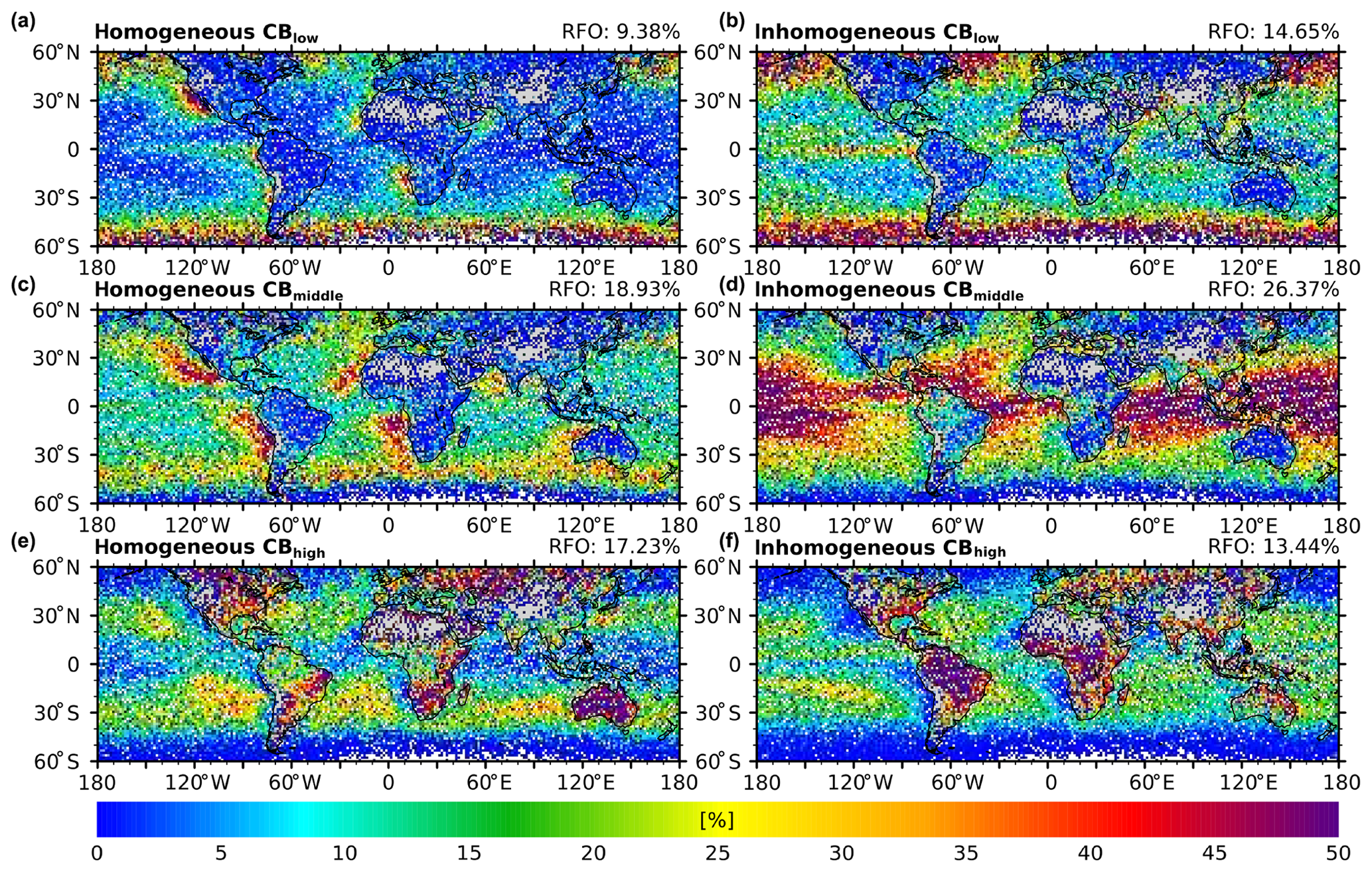
Figure 3Relative frequency of occurrence of the six cloud classes separated using the three classes of cloud-base height and two classes of cloud-top height heterogeneity. (a, b) Low, (c, d) mid-latitudes and (e, f) high clouds and (a, c, e) homogeneous (stratiform) and (b, d, f) heterogeneous (cumuliform) clouds.
3.3 Geographical distribution of the cloud regimes
The three cloud-base classes and two inhomogeneity cloud classes are now combined to define six new liquid water cloud types or cloud regimes. The global distribution of relative frequencies of occurrence (RFOs) of these cloud classes is shown in Fig. 3. Clouds with low and middle base altitude tend to be more heterogeneous, and clouds with high base altitude more are homogeneous. Low and middle clouds tend to occur over ocean rather than land, although the contrast is less strong for stratiform clouds.

Figure 4PDFs of the spatio-temporal distribution of 4 years (2007–2010) of MODIS retrievals as reported in the CCCM dataset at the 20 km × 20 km horizontal resolution at nadir below the A-Train satellite constellation, between 60∘ S and 60∘ N. Liquid clouds are selected. Light green – low, homogeneous clouds; dark green – low, heterogeneous clouds; red – middle, homogeneous clouds; purple – middle, heterogeneous clouds; light blue – high, homogeneous clouds; dark blue – high, heterogeneous clouds. (a) Droplet number concentration, Nd (cm−3); (b) liquid water path, L (g m−2).
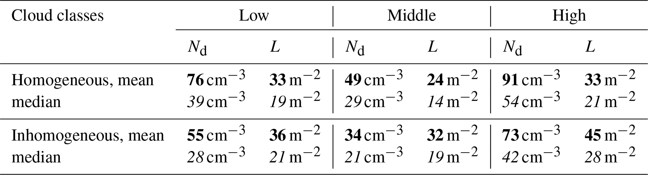
Table 1Average (bold) and median (italic) values of Nd and L for the six particular cloud classes derived from their PDFs (Fig. 4).
Most of the liquid water clouds with low Hbase are located over the ocean in the storm track regions in middle to high latitudes. Only a small amount of the low clouds occur in low latitudes. Homogeneous low clouds concentrate in mid-latitudes, especially in the Southern Hemisphere and in narrow coastal stripes west of North and South America and north and southern Africa, indicating parts of the typical stratocumulus clouds in these regions with very low Hbase. The occurrence is highest over regions with relatively low sea surface temperatures. The inhomogeneous clouds in this cloud-base class occur mainly in the mid-latitudes in both hemispheres, though a small amount can be found in tropical regions, especially along the ITCZ in the east Pacific.
Almost all mid-level-base clouds are marine clouds located over the oceans in low latitudes. Especially in the tropics along the ITCZ in the Indian Ocean and in the west Pacific, this cloud class is frequent. Inhomogeneous clouds in this cloud-base class extend in low latitudes around the entire globe, leaving out the stratocumulus decks and concentrating mainly in shallow cumulus regions and along the ITCZ.
In contrast to the cloud-base classes of lower Hbase, most of the high clouds occur over land. However, a non-negligible amount can be found over the ocean in low latitudes. Only in higher latitudes over the ocean and in the stratocumulus regions in the east Pacific and east Atlantic are almost no clouds with Hbase>950 m found. A significant amount of homogeneous clouds in this cloud-base class are located over land with maxima over southern Africa, Australia and northwest Asia. Over the ocean they cover two bands in both hemispheres at around 30∘, leaving out roughly the areas covered by the inhomogeneous mid-level-base clouds. The inhomogeneous high-base clouds occur mainly over land with maxima over rain forest regions in South America and middle Africa. Over ocean these clouds can be found equally distributed to inhomogeneous clouds in low latitudes except in the stratocumulus decks.
The key reason to define cloud regimes is that clouds are supposed to show different characteristics in these regimes. The hypothesis is that their response to perturbations, e.g. of aerosol concentrations, can possibly be identified more clearly in analyses when focusing on individual regimes (Mülmenstädt and Feingold, 2018). The goal of this section is to demonstrate the usefulness of the separation in cloud regimes according to the six classes defined in the previous section. To this end, the two main bulk cloud quantities are investigated, namely the cloud liquid water path, L, and the cloud droplet number concentration, Nd. Both are computed on the basis of the MODIS bi-spectral retrievals as reported in the CCCM dataset. Nd is computed from the retrieved cloud optical thickness and cloud-top droplet effective radius following Grosvenor et al. (2018) and the parameters defined in Quaas et al. (2006).
Cloud droplet number concentration is a key quantity when assessing aerosol–cloud interactions and cloud radiative effects (e.g. Grosvenor et al., 2018). It depends on chemical composition and size distribution of the precursor aerosol, as well as cloud-base vertical velocity (Barahona et al., 2011). It is also very much influenced by cloud and precipitation microphysical processes (Wood et al., 2012) as well as cloud-top and cloud-side entrainment.Figure 4 shows the global PDF of Nd for the six cloud regimes, and Table 1 summarises the mean and median values. The values are clearly distinct between the six classes. One key feature is that for all cloud-base heights, the homogeneous clouds contain fewer droplets than the heterogeneous ones. This is consistent with the expectation that heterogenous, convective clouds are driven by stronger updraughts. In terms of the altitude classes, low-base clouds show more droplets than mid-level-base clouds. This is a feature of the geographical distribution: both types occur mostly over oceans, but the mid-level-base clouds are more prevalent over the pristine parts of the oceans. The highest Nd is observed for the high clouds, due to the fact that high clouds mostly occur over continents.
Also in terms of liquid water path, L, the clouds in the six classes are distinct. Homogeneous, i.e. more stratiform, clouds, are thinner than the heterogeneous counterparts in each altitude class. This is consistent with the fact that convective clouds tend to develop more in the vertical, compared to stratiform clouds. Among the cloud altitude classes, L is smallest for mid-level-base clouds and largest for high clouds. Note that these clouds are only the liquid-water clouds, so that the vertical development is limited by the 0 ∘C level in our definition. Here, low clouds have the largest potential to develop in the vertical and yet remain liquid. Over land, where high cloud bases are prevalent, the 0∘ level is reached at higher altitudes, allowing these clouds to develop further in the vertical. Due to the choice made here to investigate only liquid water clouds, the behaviour is different in different latitudes and seasons, due to the fact that the freezing level is at lower heights in higher latitudes and winter. More detail of the geographical variation in the cloud regimes is provided in the Appendix, where the cloud properties for the different regimes are compared for land vs. ocean and tropics vs. extratropics.
The goal of the present study was to overcome limitations in the definition of cloud regimes. Such a definition is desirable, for example, in the context of studying aerosol–cloud interactions. Previous approaches were at the comparatively very coarse resolution of either meteorological re-analyses or used cloud parameters that are, however, the ones to study in aerosol–cloud interaction and thus cannot be used to stratify the data. Also, previous approaches were not very compatible with the standard WMO definitions. Here, we propose six cloud regimes for liquid clouds, separated by (i) cloud-base height and (ii) cloud-top height variability as an inhomogeneity parameter. Both parameters are derived from active remote sensing satellite measurements and are thus available at the scale of satellite retrievals. They are evaluated using a 4-year (2007–2010) dataset of combined A-Train satellite data in the CCCM dataset. A new approach to retrieve cloud-base altitude from spaceborne lidar has recently been developed and applied here. The geographical distributions of the frequency of occurrence of the six cloud regimes shows desirable features: oceanic and continental clouds are smoothly separated, and typical cloud regimes such as stratocumulus decks are readily identified. In order to demonstrate the usefulness of the cloud regimes, cloud parameters not used to define the regimes, but useful to study, e.g. aerosol–cloud interactions, have been analysed. The selected parameters are cloud droplet concentration and cloud liquid water path. From the analysis it is evident that the cloud regimes show different characteristics in both quantities; i.e. the cloud types are clearly distinct. In particular, expected features of homogeneous (interpreted as stratiform) and heterogeneous (interpreted as cumuliform) clouds appear, as do features related to predominant aerosol sources and boundary-layer dynamics.
In future work, the study could be enhanced to study all clouds and not just the liquid-water ones as done in the present study. While the cloud classification method could be adapted in a straightforward way, this would require a new analysis of how the classes differ in their characteristics. The current study is limited by the fact that it can only be applied to the ground track below the A-Train lidar and radar retrievals. However, approaches exist to infer cloud-base altitude from passive, multi-angle measurements as well (Böhm et al., 2019). An adaptation of our method to these swath data would allow the analysis of much larger data volumes.
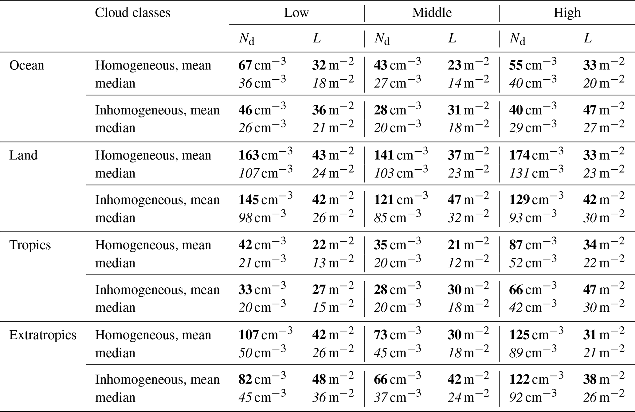
More detail about the characterisation of Nd and L by cloud regime is provided in Figs. A1 and A2 and summarised in Table A1. The PDFs of Nd (Fig. A1) and L (Fig. A2) are separated into oceanic and continental surfaces and between the tropics and extratropics, respectively. The droplet concentrations are somewhat lower over ocean compared to the global mean but are by factors of 2 to 4 higher over land (there are many more data points for liquid-water cloud retrievals over ocean than over land) in all cloud regimes, consistent with the expectation. The result of smaller Nd for inhomogeneous vs. homogeneous clouds holds for all categories over both land and ocean. Liquid water path on average is slightly lower over ocean and slightly larger over land, except for the high clouds where things are rather similar. That inhomogeneous clouds have higher L holds true over both land and ocean, with the exception of the low clouds over land. Clouds in the tropics have larger Nd than in the extratropics, and they also have larger L (except for those with high cloud bases).
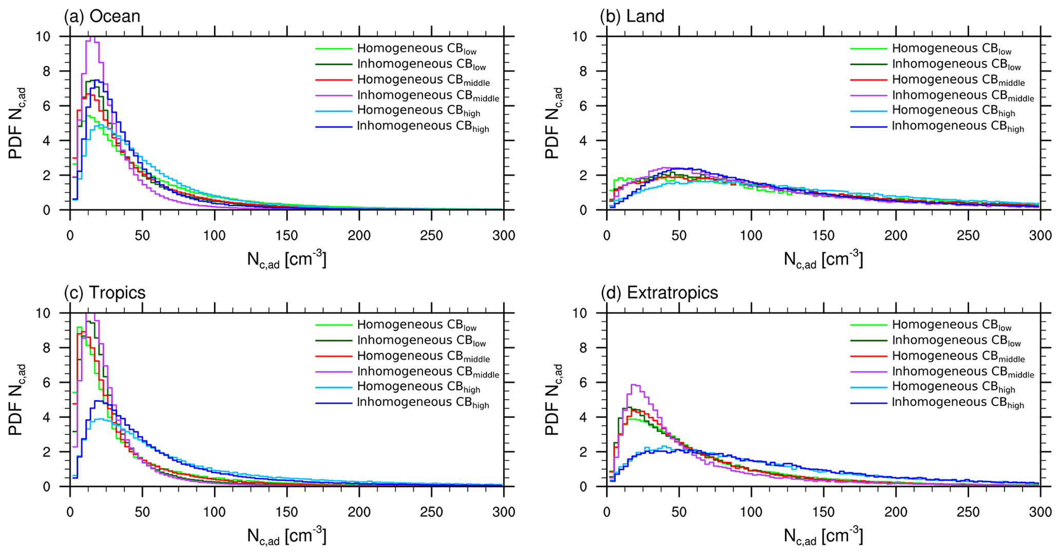
Figure A1As Fig. 4a, but separately for (a) ocean, (b) land, (c) the tropics (20∘ S–20∘ N) and (d) the extratropics (40∘ S–60∘ S and 40–60∘ N).
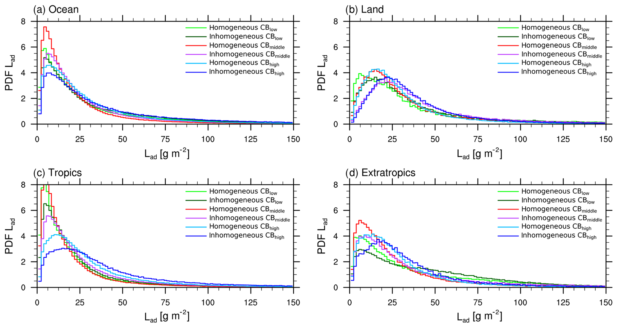
Figure A2As Fig. 4b, but separately for (a) ocean, (b) land, (c) the tropics (20∘ S–20∘ N) and (d) the extratropics (40–60∘ S and 40–60∘ N).
Table A1Average (bold) and median (italic) values of Nd and L for the six particular cloud classes derived from their PDFs, but separated, but separated for ocean, land, the tropics (20∘ S–20∘ N) and the extratropics (40–60∘ S and 40–60∘ N).
All analyses are based on the publicly available CCCM dataset (Kato et al., 2010, 2011).
CU and JQ designed the research with input from all authors. OS and JM prepared the satellite data. CU and KB performed the data analysis with support from all other authors. CU and JQ wrote the manuscript with input from all authors.
The authors declare that they have no conflict of interest.
The authors are grateful to the satellite retrieval science teams for the CALIPSO, CloudSat and MODIS instruments and in particular Seiji Kato and his coworkers at NASA Langley for compiling the CCCM dataset and helping with questions. The authors wish to thank the two anonymous reviewers for their constructive comments. We acknowledge support from Leipzig University for Open Access Publishing.
This research has been supported by the European Research Council (grant no. QUAERERE (306284)).
This paper was edited by Armin Sorooshian and reviewed by two anonymous referees.
Barahona, D., Sotiropoulou, R., and Nenes, A.: Global distribution of cloud droplet number concentration, autoconversion rate, and aerosol indirect effect under diabatic droplet activation, J. Geophys. Res., 116, D09203, https://doi.org/10.1029/2010JD015274, 2011. a
Barnes, W. L., Pagano, T. S., and Salomonson, V. V.: Prelaunch Characteristics of the Moderate Resolution Imaging Spectroradiometer (MODIS) on EOS-AM1, IEEE T. Geosci. Remote, 36, 1088–1100, https://doi.org/10.1109/36.700993, 1998. a
Bloom, S., da Silva, A., Dee, D., Bosilovich, M., J-D, Chern, Pawson, S., Schubert, S., and Sienkiewicz, M.: Documentation and Validation of the Goddard Earth Observing System (GEOS) Data Assimilation System-Version 4, Technical Report Series on Global Modeling and Data Assimilation, 26, 112 pp., NASA/TM–2005–104 606, 2005. a
Böhm, C., Sourdeval, O., Mülmenstädt, J., Quaas, J., and Crewell, S.: Cloud base height retrieval from multi-angle satellite data, Atmos. Meas. Tech., 12, 1841–1860, https://doi.org/10.5194/amt-12-1841-2019, 2019. a
Bony, S., Dufresne, J.-L., Treut, H. L., Morcrette, J.-J., and Senior, C.: On dynamic and thermodynamic components of cloud changes, Clim. Dynam., 22, 71–86, 2004. a
Boucher, O., Randall, D., Artaxo, P., Bretherton, C., Feingold, G., Forster, P., Kerminen, V.-M., Kondo, Y., Liao, H., Lohmann, U., Rasch, P., Satheesh, S., Sherwood, S., Stevens, B., and Zhang, X.: Clouds and Aerosols, in: Climate Change 2013: The Physical Science Basis, Contribution of Working Group I to the Fifth Assessment Report of the Intergovernmental Panel on Climate Change, edited by: Stocker, T., Qin, D., Plattner, G.-K., Tignor, M., Allen, S., Boschung, J., Nauels, A., Xia, Y., Bex, V., and Midgley, P., Cambridge University Press, Cambridge, United Kingdom and New York, NY, USA, 571–657, https://doi.org/10.1017/CBO9781107415324.016, 2013. a
Dhuria, H. L. and Kyle, H. L.: Cloud Types and the Tropical Earth Radiation Budget, J. Clim., 3, 1409–1434, https://doi.org/10.1175/1520-0442(1990)003<1409:CTATTE>2.0.CO;2, 1990. a
Grosvenor, D. P., Sourdeval, O., Zuidema, P., Ackerman, A., Alexandrov, M. D., Bennartz, R., Boers, R., Cairns, B., Chiu, C., Christensen, M., Deneke, H., Diamond, M., Feingold, G., Fridlind, A., Hünerbein, A., Knist, C., Kollias, P., Marshak, A., McCoy, D., Merk, D., Painemal, D., Rausch, J., Rosenfeld, D., Russchenberg, H., Seifert, P., Sinclair, K., Stier, P., B. van D., Wendisch, M., Werner, F., Wood, R., Zhang, Z., and Quaas, J.: Remote sensing of cloud droplet number concentration in warm clouds: A review of the current state of knowledge and perspectives, Rev. Geophys., 56, 409–453, https://doi.org/10.1029/2017RG000593, 2018. a, b, c
Gryspeerdt, E. and Stier, P.: Regime-based analysis of aerosol-cloud interactions, Geophys. Rev. Lett., 39, L21802, https://doi.org/10.1029/2012GL053221, 2012. a
Gryspeerdt, E., Goren, T., Sourdeval, O., Quaas, J., Mülmenstädt, J., S., D., Unglaub, C., Gettelman, A., and Christensen, M.: Constraining the aerosol influence on cloud liquid water path, Atmos. Chem. Phys., 19, 5331–5347, https://doi.org/10.5194/acp-19-5331-2019, 2019. a
Hartmann, D. L., Ockert-Bell, M. E., and Michelsen, M. L.: The Effect of Cloud Type on Earth's Energy Balance: Global Analysis, J. Clim., 5, 1281–1304, https://doi.org/10.1175/1520-0442(1992)005<1281:TEOCTO>2.0.CO;2, 1992. a
Haynes, J. M., L'Ecuyer, T. S., Stephens, G. L., Miller, S. D., Mitrescu, C., Wood, N. B., and Tanelli, S.: Rainfall retrieval over the ocean with spaceborne W-band radar, J. Geophys. Res., 114, D00A22, https://doi.org/10.1029/2008JD009973, 2009. a
Howard, L.: Essay on the modifications of clouds, John Churchill & Sons, London, 64 pp., 1803. a
Jakob, C., Tselioudis, G., and Hume, T.: The Radiative, Cloud, and Thermodynamic Properties of the Major Tropical Western Pacific Cloud Regimes, J. Clim., 18, 1203–1215, https://doi.org/10.1175/JCLI3326.1, 2005. a, b
Kato, S., Sun-Mack, S., Miller, W. F., Rose, F. G., Chen, Y., Minnis, P., and Wielicki, B. A.: Relationships among cloud occurrence frequency, overlap, and effective thickness derived from CALIPSO and CloudSat merged cloud vertical profiles, J. Geophys. Res., 115, D00H28, https://doi.org/10.1029/2009JD012277, 2010. a, b, c
Kato, S., Rose, F. G., Sun-Mack, S., Miller, W. F., Chen, Y., Rutan, D. A., Stephens, G. L., Loeb, N. G., Minnis, P., Wielicki, B. A., Winker, D. M., Charlock, T. P., Stackhouse Jr., W., Xu, K.-M., and Collins, W. D.: Improvements of top-of-atmosphere and surface irradiance computations with CALIPSO-, CloudSat-, and MODIS-derived cloud and aerosol properties, J. Geophys. Res., 116, D19209, https://doi.org/10.1029/2011JD016050, 2011. a, b, c
Kato, S., Miller, W. F., Sun-Mack, S., Rose, F. G., Chen, Y., and Mlynczak, P. E.: Variable Descriptions of the A-Train Integrated CALIPSO, CloudSat, CERES, and MODIS Merged Product (CCCM or C3M), available at: https://eosweb.larc.nasa.gov/project/ceres/readme/c3m_variables_B1_v2.pdf (last access: 9 March 2016), 2014. a
King, M. D., Menzel, W. P., Kaufman, Y. J., Tanre, D., Bo-Cai, G., Platnick, S., Ackerman, S. A., Remer, L. A., Pincus, R., and Hubanks, P. A.: Cloud and Aerosol Properties, Precipitable Water, and Profiles of Temperature and Water Vapor from MODIS, IEEE Trans. Geosci. Remote, 41, 442–458, https://doi.org/10.1109/TGRS.2002.808226, 2003. a
Klein, S. and Hartmann, D.: The seasonal cycle of low stratiform clouds, J. Clim., 6, 1587–1606, https://doi.org/10.1175/1520-0442(1993)006<1587:TSCOLS>2.0.CO;2, 1993. a
Medeiros, B. and Stevens, B.: Revealing differences in GCM representations of low clouds, Clim. Dynam., 36, 385–399, https://doi.org/10.1007/s00382-009-0694-5, 2011. a
Mülmenstädt, J. and Feingold, G.: The radiative forcing of aerosol-cloud interactions in liquid clouds: Wrestling and embracing uncertainty, Curr. Clim. Change Rep., 4, 23–40, https://doi.org/10.1007/s40641-018-0089-y, 2018. a, b, c
Mülmenstädt, J., Sourdeval, O., Henderson, D. S., L'Ecuyer, T. S., Unglaub, C., Jungandreas, L., Böhm, C., Russell, L. M., and Quaas, J.: Using CALIOP to estimate cloud-field base height and its uncertainty: The Cloud Base Altitude Spatial Extrapolator (CBASE) algorithm and dataset, Earth Syst. Sci. Data, 10, 2279–2293, https://doi.org/10.5194/essd-10-2279-2018, 2018. a, b, c, d
Nam, C. C. and Quaas, J.: Geographically versus dynamically defined boundary layer cloud regimes and their use to evaluate general circulation model cloud parameterizations, Geophys. Res. Lett., 40, 4951–4956, https://doi.org/10.1002/grl.50945, 2013. a
Norris, J. R. and Weaver, C. P.: Improved Techniques for Evaluating GCM Cloudiness Applied to the NCAR CCM3, J. Clim., 14, 2540–2550, https://doi.org/10.1175/1520-0442(2001)014<2540:ITFEGC>2.0.CO;2, 2001. a
Oreopoulos, L. and Cahalan, R. F.: Cloud Inhomogeneity from MODIS, J. Clim., 18, 5110–5124, https://doi.org/10.1175/JCLI3591.1, 2005. a
Painemal, D. and Zuidema, P.: Assessment of MODIS cloud effective radius and optical thickness retrievals over the Southeast Pacific with VOCALS-REx in situ measurements, J. Geophys. Res., 116, D24206, https://doi.org/10.1029/2011JD016155, 2011. a
Park, S. and Shin, J.: Heuristic estimation of low-level cloud fraction over the globe based on a decoupling parameterization, Atmos. Chem. Phys., 19, 5635–5660, https://doi.org/10.5194/acp-19-5635-2019, 2019. a
Platnick, S.: Vertical photon transport in cloud remote sensing problems, J. Geophys. Res., 105, 22919–22935, https://doi.org/10.1029/2000JD900333, 2002. a
Platnick, S., King, M. D., Ackerman, S. A., Menzel, W. P., Baum, B. A., Riedi, J. C., and Frey, R. A.: The MODIS cloud products: algorithms and examples from Terra, IEEE Trans. Geosci. Remote, 41, 459–473, https://doi.org/10.1109/TGRS.2002.808301, 2003. a, b
Quaas, J., Boucher, O., and Lohmann, U.: Constraining the total aerosol indirect effect in the LMDZ and ECHAM4 GCMs using MODIS satellite data, Atmos. Chem. Phys., 6, 947–955, https://doi.org/10.5194/acp-6-947-2006, 2006. a
Rienecker, M., Suarez, M., Todling, R., Bacmeister, J., Takacs, L., Liu, H.-C., Gu, W., Sienkiewicz, M., Koster, R., Gelaro, R., Stajner, I., and Nielsen, J.: The GEOS-5 Data Assimilation System-Documentation of Versions 5.0.1, 5.1.0, and 5.2.0, Technical Report Series on Global Modeling and Data Assimilation, 27, 118 pp., NASA/TM–2008–104 606, 2008. a
Ringer, M. A. and Allan, R. P.: Evaluating climate model simulations of tropical cloud, Tellus A, 56, 308–327, https://doi.org/10.1111/j.1600-0870.2004.00061.x, 2004. a
Rossow, W. B. and Schiffer, R. A.: Advances in Understanding Clouds from ISCCP, B. Am. Meteorol. Soc., 80, 2261–2287, https://doi.org/10.1175/1520-0477(1999)080<2261:AIUCFI>2.0.CO;2, 1999. a, b
Shin, J. and Park, S.: The Relationship between Low-Level Cloud Amount and Its Proxies over the Globe by Cloud Types, Atmos. Chem. Phys. Discuss., https://doi.org/10.5194/acp-2019-560, in review, 2019. a
Stephens, G., Winker, D., Pelon, J., Trepte, C., Vane, D., Yuhas, C., L'Ecuyer, T., and Lebsock, M.: CloudSat and CALIPSO within the A-Train: Ten years of actively observing the Earth system, B. Am. Meteorol. Soc., 99, 569–581, https://doi.org/10.1175/BAMS-D-16-0324.1, 2018. a
Stephens, G. L., Vane, D. G., Boain, R. J., Mace, G. G., Sassen, K., Wang, Z., Illingworth, A. J., O'Connor, E. J., Rossow, W. B., Durden, S. L., Miller, S. D., Austin, R. T., Benedetti, A., Mitrescu, C., and TEAM, T. C. S.: THE CLOUDSAT MISSION AND THE A-TRAIN: A New Dimension of Space-Based Observations of Clouds and Precipitation, B. Am. Meteorol. Soc., 83, 1771–1790, https://doi.org/10.1175/BAMS-83-12-1771, 2002. a
Stephens, G. L., Vane, D. G., Tanelli, S., Im, E., Durden, S., Rokey, M., Reinke, D., Partain, P., Mace, G. G., Austin, R., L'Ecuyer, T., Haynes, J., Lebsock, M., Suzuki, K., Waliser, D., Wu, D., Kay, J., Gettelman, A., Wang, Z., and Marchand, R.: CloudSat mission: Performance and early science after the first year of operation, J. Geophys. Res., 113, D00A18, https://doi.org/10.1029/2008JD009982, 2008. a, b, c
Stevens, B. and Feingold, G.: Untangling aerosol effects on clouds and precipitation in a buffered system, Nature, 461, 607–613, https://doi.org/10.1038/nature08281, 2009. a
Su, W., Loeb, N. G., Xu, K., Schuster, G. L., and Eitzen, Z. A.: An estimate of aerosol indirect effect from satellite measurements with concurrent meteorological analysis, J. Geophys. Res., 115, D18219, https://doi.org/10.1029/2010JD013948, 2010. a
Tanelli, S., Durden, S. L., Im, E., Pak, K., Reinke, D., Partain, P., Haynes, J., and Marchand, R.: CloudSat's Cloud Profiling Radar After Two Years in Orbit: Performance, Calibration, and Processing, IEEE Trans. Geosci. Remote, 46, 3560–3573, https://doi.org/10.1109/TGRS.2008.2002030, 2008. a
Tselioudis, G., Zhang, Y., and Rossow, W. B.: Cloud and Radiation Variations Associated with Northern Midlatitude Low and High Sea Level Pressure Regimes, J. Clim., 13, 312–327, https://doi.org/10.1175/1520-0442(2000)013<0312:CARVAW>2.0.CO;2, 2000. a
Williams, K. D. and Webb, M. J.: A quantitative performance assessment of cloud regimes in climate models, Clim. Dynam., 33, 141–157, https://doi.org/10.1007/s00382-008-0443-1, 2008. a
Winker, D. M., Hunt, W. H., and McGill, M. J.: Initial performance assessment of CALIOP, Geophys. Res. Lett., 34, L19803, https://doi.org/10.1029/2007GL030135, 2007. a, b, c
Winker, D. M., Vaughan, M. A., Omar, A., Hu, Y., and Powell, K. A.: Overview of the CALIPSO Mission and CALIOP Data Processing Algorithms, J. Atmos. Ocean. Tech., 26, 2310–2323, https://doi.org/10.1175/2009JTECHA1281.1, 2009. a
WMO: International cloud atlas, volume I – manual on the observation of clouds and other meteors, available at: https://cloudatlas.wmo.int/docs/wmo_407_en-v1.pdf (last access: 27 February 2020), 1975. a, b, c
WMO: International cloud atlas, available at: https://cloudatlas.wmo.int (last access: 27 February 2020), 2017. a, b
Wood, R. and Bretherton, C.: On the relationship between stratiform low cloud cover and lower-tropospheric stability, J. Clim., 19, 6425–6432, https://doi.org/10.1175/JCLI3988.1, 2006. a
Wood, R., Leon, D., Lebsock, M., Snider, J., and Clarke, A. D.: Precipitation driving of droplet concentration variability in marine low clouds, J. Geophys. Res., 117, D19210, https://doi.org/10.1029/2012JD018305, 2012. a
Zeng, S., Cornet, C., Parol, F., Riedi, J., and Thieuleux, F.: A better understanding of cloud optical thickness derived from the passive sensors MODIS/AQUA and POLDER/PARASOL in the A-Train constellation, Atmos. Chem. Phys., 12, 11245–11259, https://doi.org/10.5194/acp-12-11245-2012, 2012. a
- Abstract
- Introduction
- Satellite data
- Definition of the cloud classes
- Cloud properties in the six cloud regimes
- Summary and conclusions
- Appendix A: Regime analysis by large-scale region
- Data availability
- Author contributions
- Competing interests
- Acknowledgements
- Financial support
- Review statement
- References