the Creative Commons Attribution 4.0 License.
the Creative Commons Attribution 4.0 License.
 | 21 Feb 2020
Accurate 3-D radiative transfer simulation of spectral solar irradiance during the total solar eclipse of 21 August 2017
Paul Ockenfuß
Claudia Emde
Bernhard Mayer
Germar Bernhard
We calculate the variation of spectral solar irradiance in the umbral shadow of the total solar eclipse of 21 August 2017 and compare it to observations. Starting from the Sun's and Moon's positions, we derive a realistic profile of the lunar shadow at the top of the atmosphere, including the effect of solar limb darkening. Subsequently, the Monte Carlo model MYSTIC (Monte Carlo code for the phYSically correct Tracing of photons In Cloudy atmospheres) is used to simulate the transfer of solar radiation through the Earth's atmosphere. Among the effects taken into account are the atmospheric state (pressure, temperature), concentrations of major gas constituents and the curvature of the Earth, as well as the reflectance and elevation of the surrounding area. We apply the model to the total solar eclipse on 21 August 2017 at a position located in Oregon, USA, where irradiance observations were performed for wavelengths between 306 and 1020 nm. The influence of the surface reflectance, the ozone profile, the mountains surrounding the observer and aerosol is investigated. An increased sensitivity during totality is found for the reflectance, aerosol and topography, compared to non-eclipse conditions. During the eclipse, the irradiance at the surface not only depends on the total ozone column (TOC) but also on the vertical ozone distribution, which in general complicates derivations of the TOC from spectral surface irradiance. The findings are related to an analysis of the prevailing photon path and its difference compared to non-eclipse conditions. Using the most realistic estimate for each parameter, the model is compared to the irradiance observations. During totality, the relative difference between model and observations is less than 10 % in the spectral range from 400 to 1020 nm. Slightly larger deviations occur in the ultraviolet range below 400 and at 665 nm.
- Article
(7611 KB) - Full-text XML
-
Supplement
(120 KB) - BibTeX
- EndNote


When modeling real world processes, we generally want to achieve one of two main goals: if measurements have not yet been performed, we can use the simulation to make predictions about the expected outcome and give recommendations for the experimental setup. If however, measured data exist, we can validate and enhance our conceptual understanding of the phenomenon under investigation by comparison with the model results. In this case, one can also use the measurements to verify the model itself, in order to increase the credibility of model predictions. The following study is carried out for all of these purposes.
In the past, the influence of a solar eclipse on surface radiation measurements and the derived state of the atmosphere were discussed in several studies. Zerefos et al. (2000) performed measurements in the UV domain during the total solar eclipse in 1999 over Europe. They discussed the implications of solar limb darkening and the ratio of diffuse to direct irradiance during a solar eclipse on ozone measurements.
Kazantzidis et al. (2007) further examined the temporal change in the wavelength ratios for ultraviolet and visible wavelengths. Along with this study, the radiative transfer model MYSTIC (Monte Carlo code for the phYSically correct Tracing of photons In Cloudy atmospheres; Mayer, 2009; Emde and Mayer, 2007) was used to model the observations in three dimensions for the first time. The wavelengths discussed were 312, 340 and 380 nm. During totality, the 3-D model reproduced the measured irradiance at 380 nm with up to 5 % accuracy, but deviated from the measurements by a factor of 3 for 312 nm. Kazantzidis et al. (2007) pointed out that the ozone profile and the surrounding topography could possibly influence surface irradiance, which was not yet included in their model. The detailed model functionality is described in Emde and Mayer (2007), where the usefulness of a total solar eclipse to validate 3-D radiative transfer codes was pointed out as well; e.g., in contrast to large-scale cloud fields, the shape of the lunar shadow exhibits a very well defined geometry, and therefore allows for an accurate representation of the reality within the model. Moreover, a 3-D model is essential to simulate irradiance in the umbral shadow, where every detected photon has to be scattered from regions outside the shadow towards the observer.
For the total solar eclipse over North America on 21 August 2017, different groups performed irradiance measurements, e.g., Calamas et al. (2018) and Bernhard and Petkov (2019). The latter measured solar irradiance at 14 different wavelengths between 306 and 1020 nm with a sensitivity high enough to yield significant results, including during totality. In their publication, they discussed the time outside the totality, i.e., the pre-umbra region, extensively, concluding that changes in the ozone column derived from spectral irradiance measurements reported in previous studies could potentially be attributed to uncertainties in the limb darkening parametrization. The importance of limb darkening, in particular when deriving ozone, is also supported by findings from Groebner et al. (2017) for the solar eclipse on 20 March 2015. To obtain a general overview of the results from many studies on atmospheric changes caused by solar eclipses, the reader is referred to Aplin et al. (2016)
In this study, we perform 3-D model calculations for the conditions during the observations at totality by Bernhard and Petkov (2019). The comparison of the modeling results to the observations is a validation of our 3-D radiative transfer model from ultraviolet to near-infrared. Moreover, we continue the work of Emde and Mayer (2007) and Kazantzidis et al. (2007) by analyzing the model's sensitivity towards changes in the ozone column and profile, as well as the surface reflectance, topography and aerosol, in order to understand how the environmental conditions influence the radiative fluxes during totality. Altogether, this provides us with the ability to precisely estimate the time evolution of radiative fluxes for the eclipse analyzed here and for future eclipses. Where this becomes important is during the totality, when the Sun is completely covered by the lunar disk. Because intensities are reduced by up to 4 orders of magnitude compared to the uncovered Sun, common measurement devices often operate close to their detection limit. Astronomical devices could produce better results at this time, but due to their high sensitivities, they would have to be protected as soon as intensities start to increase again, which can be a matter of only a few minutes or seconds. Therefore, pre-estimating irradiance in advance is crucial to preparing measurement campaigns.
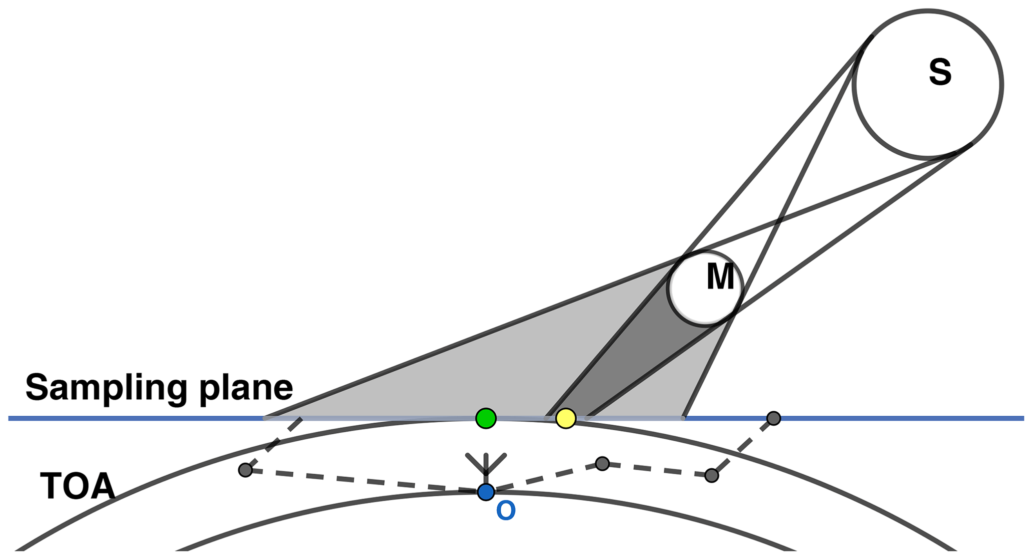
Figure 1Schematic illustration of a solar eclipse, including umbral (dark gray) and penumbral (light gray) shadow and the definition of sampling plane and top of atmosphere (TOA). S denotes the Sun, M the Moon and O the observer. The green dot marks the point in the sampling plane located vertically above the observer. The yellow dot represents the intersection of the observer–Sun line with the sampling plane. The dashed lines show exemplary photon paths. In the atmospheric part, the solar angle is assumed to be constant, atmospheric refraction is neglected.
The basis for modeling irradiances during totality of the solar eclipse is the Monte Carlo solver MYSTIC (Mayer, 2009) with alterations from a previous study (Emde and Mayer, 2007). MYSTIC is operated as one of several radiative transfer solvers of the libRadtran package (http://www.libradtran.org, last access: 20 December 2019; Mayer and Kylling, 2005; Emde et al., 2016). We enhanced and generalized this model in different aspects to make calculations at arbitrary observer positions on Earth possible. In general, the simulation process can be divided into two distinct parts: in the celestial part, we calculate the distribution of solar irradiance under eclipse conditions in a plane tangential to the top of atmosphere (TOA) for given positions of the Sun and Moon. We call this plane the “sampling plane” (SP), as illustrated in Fig. 1. In the atmospheric part, the Monte Carlo model is used to determine the relative influence of every pixel in the sampling plane on the measured result at the observer position under non-eclipse conditions. This function is called the “contribution function” (C). Multiplication of the contribution function with the irradiance distribution and subsequent summation yields the final model result. In this approach, the atmospheric part, which is costly to simulate, depends only on the solar position. Therefore, it is sufficient to calculate this part only once for the total eclipse with a duration typically around 2 min. The fast movement of the lunar shadow is contained in the easier-to-calculate celestial part.

Figure 2Graphical illustration (not to scale) of the Sun and Moon with definitions of various geometrical quantities. RS, PM and PS are obtained from JPL Horizons and allow calculation of RM and X for arbitrary d.
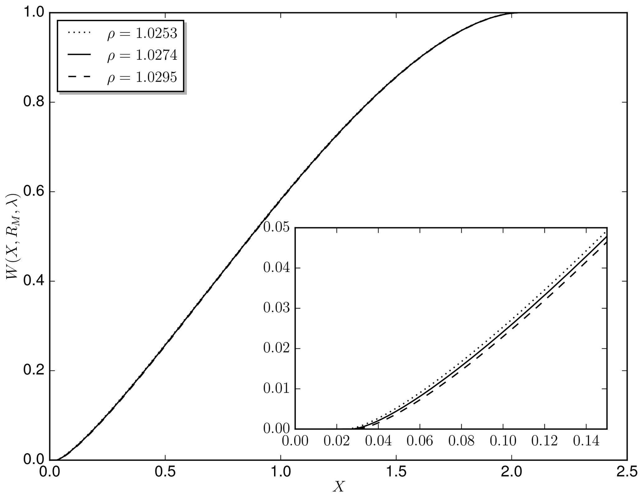
Figure 3The relative solar irradiance compared to the uncovered Sun, calculated for λ=555 nm with the limb darkening parametrization from Pierce and Slaughter (1977) for different .
2.1 Celestial part
Ephemeris data of the Sun and Moon were gathered using the method of Giorgini et al. (1996). The described service provides access to the JPL Horizons system operated by the Solar System and Dynamics Group of the Jet Propulsion Laboratory (JPL). It allows for creating ephemeris for various celestial bodies in the solar system for arbitrary times and observer positions on Earth. The data we used were azimuth, elevation, angle diameter and distance from observer respectively for the Sun and Moon. These quantities can be interpreted as spherical coordinates of the Sun and Moon in a local coordinate system centered at the observer. The calculation of extraterrestrial solar irradiance for a given position, time and wavelength λ was done following the geometrical considerations in Koepke et al. (2001). The basic idea is to integrate the solar irradiance over the visible part of the solar disk, i.e., the part which is not covered by the lunar disk. The key quantities in the calculation of the relative solar irradiance are the celestial distance X of solar and lunar disk and the radius of the lunar disk RM. For this and all further calculations, celestial distances are always measured in radii of the solar disk RS, where RS is the angle radius of the solar disk in arcseconds. An overview over the definition of the different geometrical quantities we use is given in Fig. 2. In order to obtain the celestial distance X(d,t) at arbitrary positions d relative to the observer, we have to calculate the angle between the position vectors of the Sun and Moon as seen from d. We obtain the following:
with PS(t) and PM(t) the position vectors of the Sun and Moon relative to the observer at time t. While the information about the shape of the lunar shadow is mainly contained in the spatial variation of X, the variation of RM(d,t) provides a small correction. An expression can be derived from the geometry shown in Fig. 2 with the distance of the Moon and the actual lunar radius which was set to RadM=1737.4 km (Archinal et al., 2018).
Evaluating Eq. (2) directly at the observer position (d=0) shows a maximum deviation of 0.02 arcsec from the angle diameter predicted directly by JPL Horizons. Evaluations at 500 km distance from the observer change the lunar radius by ±1 arcsec. For the Sun, a similar calculation shows that the relative change of the disk radius due to movements in the sampling plane is of the order 10−6 because of the much greater distance to the Earth, so it is safe to set . Because every evaluation of requires an expensive numerical integration over the visible solar disk, in the first step we precalculate w for 4000 values of X and nine values of RM. In the second step, we calculate X(d,t) and RM(d,t) for every pixel in the sampling plane and obtain w through linear interpolation. In Fig. 3, is shown for λ=555 nm at time 17:20:00 UTC.
An important fact one has to consider when integrating over the visible part of the solar disk is the darkening towards the outside of the disk. The cause is that the Sun has a diffuse border with an optical thickness like an atmosphere. Looking directly at the center, we can see to deeper and therefore hotter layers than looking at the rim. The parametrization for this “limb darkening” effect used by Koepke et al. (2001) is based on theoretical considerations from Waldmeier (1955). For our study, we follow the recommendations by Bernhard and Petkov (2019) and implemented the more accurate parametrization developed by Pierce et al. (1977), based on two measurement campaigns (Pierce and Slaughter, 1977; Pierce et al., 1977). The limb darkening factor Γ describes the radiance relative to the center of the solar disk and is expressed as a fifth-degree polynomial in μ=cos (Ψ(r)). Definition of Ψ is shown in Fig. 4. For discrete wavelengths from 303 to 730 nm coefficients are taken from Pierce and Slaughter (1977) (Table IV) and for wavelengths from 740 to 1047 nm from Pierce et al. (1977) (Table IV). These values are interpolated linearly. The effect of limb darkening for different wavelengths is illustrated in Fig. 5.
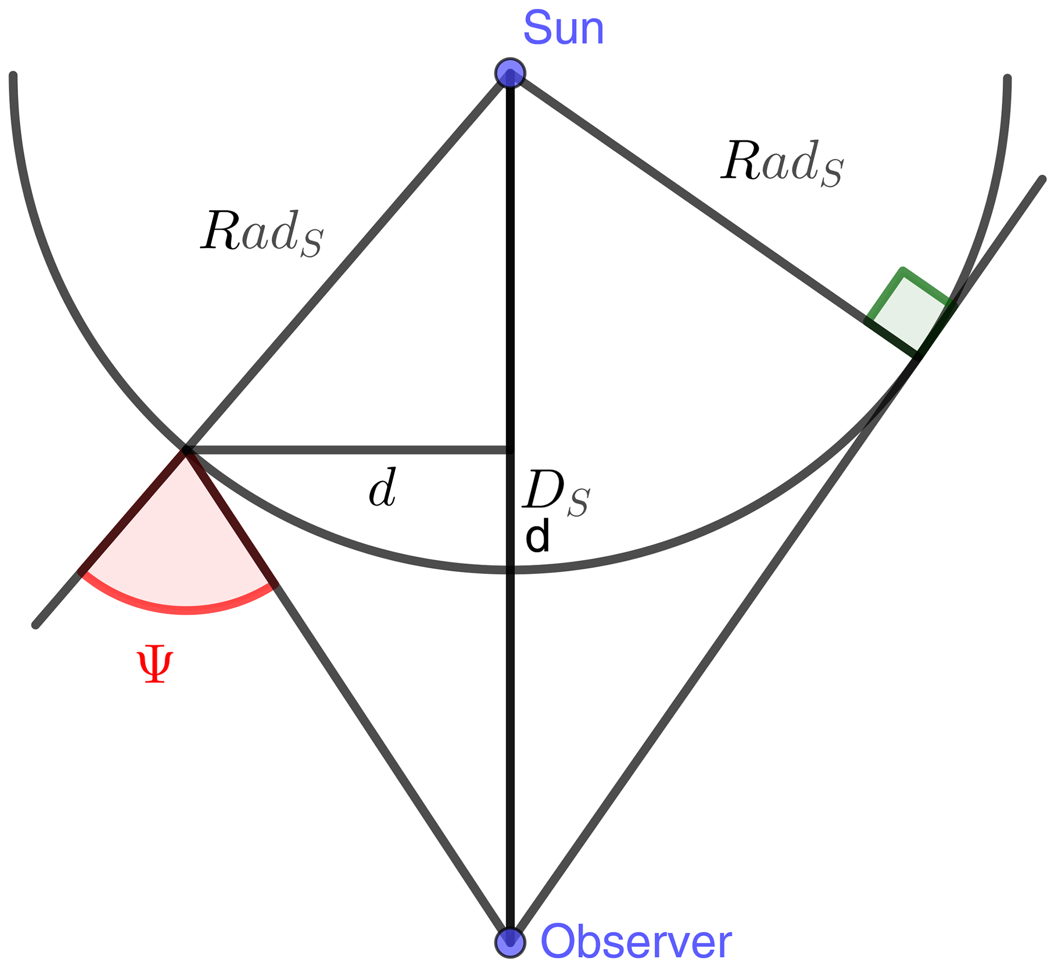
Figure 4Definition of the angle Ψ used in the equations for the limb darkening coefficient. If d, DS and RadS=695.700 km are given, it is possible to derive Ψ using simple trigonometric relations.
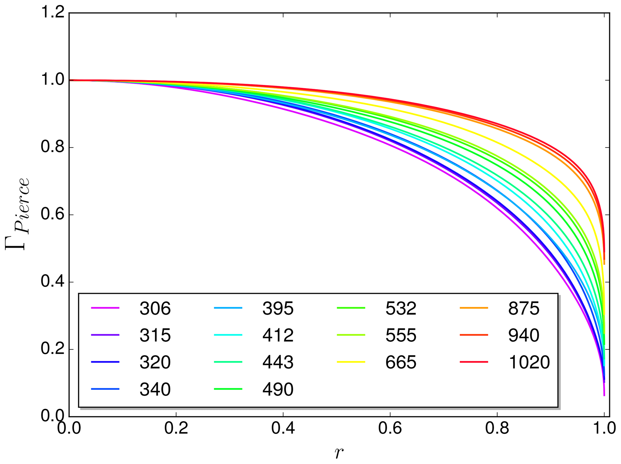
Figure 5Values of the limb darkening factor Γ based on Pierce and Slaughter (1977) and Pierce et al. (1977). Curves are for different wavelengths, given in nanometers. r denotes the position on the visible solar disk, with r=0 at the center and r=1 at the limb.
2.2 Atmospheric part
To obtain the two-dimensional contribution function C at the TOA, the fully spherical 3-D Monte Carlo solver MYSTIC was applied. For the details of this part of the simulation process, the reader is referred to Emde and Mayer (2007). In this setup, the photons are starting from the observer and traced backwards through the atmosphere (due to the reversibility of light paths, this is equivalent to tracing them from the Sun to the observer). If a photon hits one of the domain boundaries, it is destroyed. This is necessary, because in spherical geometry, periodic boundary conditions are not applicable, unless the whole planet is simulated. We ensure that the boundaries have no implications on the result by use of a sufficiently large domain.
If a photon leaves the TOA in the direction of the Sun, it is traced further to the sampling plane (see Fig. 1), where it is counted at the incident position. Averaging over many photons, this creates a map of contributions, i.e., how much every point in the sampling plane contributes to the irradiance at the observer position. We call this map the contribution function .
To speed up the convergence, the “local estimate technique” (Marshak and Davis, 2005) is applied.
2.3 Modeled irradiance at location of observer
With both the solar irradiance weighting function and the contribution function available, we are now finally able to bring the parts together to obtain the irradiance at the sensor position. Summing up the product of w and C for every point in the sampling plane yields the diffuse fraction of the sunlight reaching the sensor. Because, for partial eclipse conditions, the light of the Sun reaching the sensor directly without any scattering in the atmosphere is not included in the inverse Monte Carlo results, we have to add it as an extra term . The exponential factor describes the direct atmospheric transmittance, depending on the total optical thickness τ which is obtained using libRadtran. d0 is the position where the line from the observer to the Sun intersects the sampling plane. Multiplying the sum of direct and diffuse fraction of sunlight at the observer position with the extraterrestrial spectrum (ETS) under non-eclipse conditions, finally gives the values we were looking for. The factor κ(t) corrects the ETS for variations in the Earth–Sun distance by use of the formula from Iqbal (1983), evaluated for 21 August. The final expression reads
2.4 The eclipse of 2017
In the following, we will apply the model to simulate solar irradiance for the total solar eclipse of 2017 at a location in Smith Rock State Park near Terrebonne, Oregon. Irradiance measurements from this site are available from Bernhard and Petkov (2019). At first, we will rebuild the environmental and atmospheric conditions at the measurement site, starting from a basic setup which will serve as a proof of concept. Stepwise, we will go on to more specific settings and analyze their sensitivity towards the result. Finally, we will simulate time series of solar irradiance for the measured wavelengths and compare them to the observed values.
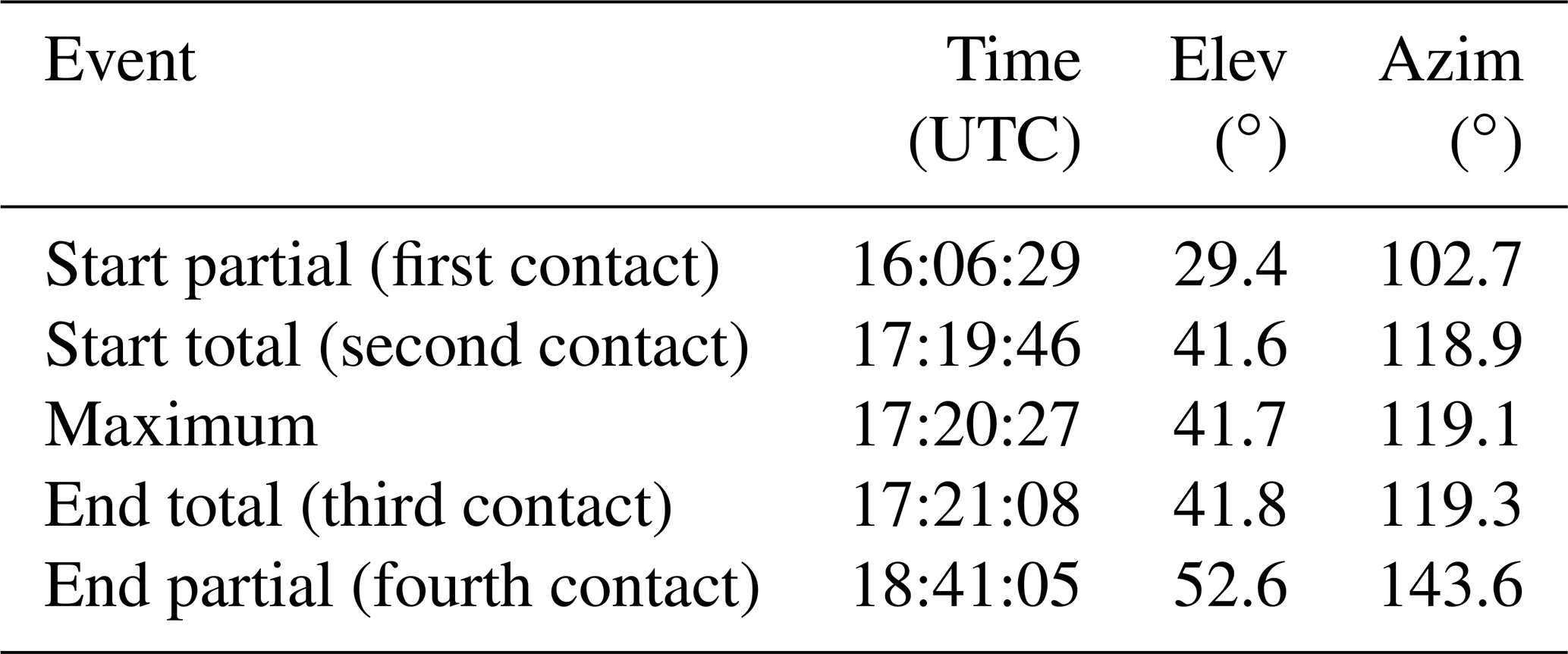
The eclipse of 2017 occurred on 21 August in the Northern Hemisphere, with the umbral shadow starting in the central Pacific, passing over the area of the United States and finally going further across two-thirds of the Atlantic Ocean. The penumbral shadow hit the US western coastline at about 16:00 UTC, before the umbral shadow had its first contact with the Earth in the Pacific at 16:48 UTC. In the following, all times will be given in UTC. Measurements were taken at 121∘08′22.8′′ W and 44∘21′46.6′′ N. At this location, approximately 37 km away from the umbral shadow's center line, the totality started at 17:19:46 UTC and lasted for 82 s. The detailed start and end times at the measurement site can be obtained from Table 1. The ratio of lunar and solar disk radius varies for the time of the partial eclipse between 1.0250 and 1.0290. The diameters of the minor axis of the elliptical shadow was calculated as 3436 km for the penumbral shadow at the time of totality, and 94 km for the umbral shadow.
The celestial data were created with JPL Horizons at the position 121∘08′22.8′′ W, 44∘21′46.6′′ N and an altitude of 866.8 m. From 14:30 until 20:00 UTC values were taken every 120 s, while from 17:10 until 17:30 UTC, the time around the totality, a higher resolution of 5 s was chosen. Up to 675.5 nm the spectrum 2004JD004937-ETS_GUEYMARD described in Bernhard et al. (2004) and available at http://uv.biospherical.com/Version2/Paper/2004JD004937-ETS_GUEYMARD.txt (last access: 20 December 2019) was used. Above 675.5 nm, the extraterrestrial spectrum published by Gueymard (2004) was used. Both were corrected for day 233 of 2017 (21 August). Profiles of pressure, temperature, density and the major gas concentrations (O3, O2, H2O, CO2, NO2) were taken from the midlatitude summer profiles by Anderson et al. (1986). The thereby specified molecular ozone profile was scaled to a total ozone column of 298 DU, corresponding to the value derived in Bernhard and Petkov (2019). The other profiles are not modified and aerosol is not included. Following the experience of Emde and Mayer (2007), a sampling grid of 2000×2000 km was used in the horizontal with a 1 km step size for the contribution function at TOA. 107 photons were traced for each wavelength.
3.1 Time series
Figure 6 gives an overview over the change of irradiance with time between 10 min before and after totality. As described above, the celestial part was fully time resolved, including the Sun's position. The atmospheric part is based on one Monte Carlo simulation at 17:20:00 UTC. Comparing it with Fig. 13 in Emde and Mayer (2007), we can see the same qualitative behavior. All wavelengths undergo a sudden drop as soon as totality occurs. The spectral irradiance of the 315 nm wavelength is remarkably lower than the visible irradiances, which is mainly due to the naturally lower irradiance values under non-eclipse conditions. The strong increase of the Rayleigh scattering cross section towards shorter wavelengths is the reason for the stronger variation in irradiance during the totality period between 17:19 and 17:21 UTC at 315 nm. Looking at the 875 nm near-infrared wavelength, one finds that it decreases by nearly 4 orders of magnitude, leading to totality intensities almost as low as in the UV part of the spectrum around 315 nm. The reason is again the proportionality of the Rayleigh scattering cross section to , making the scattering into the umbral shadow much less efficient for near-infrared radiation than it is for shorter wavelengths. For all wavelengths, there is a slight asymmetry in the irradiance gradient at the beginning and at the end of the eclipse. This can be explained similarly to the arguments for radiance in Emde and Mayer (2007), with the contribution function at TOA. Most of the diffuse photons originate from the vicinity of a line (black in Fig. 7) at TOA between the point directly above the observer (green dot in Fig. 7) and the intersection point of the observer–Sun line with the TOA (yellow dot). The histogram in Fig. 7 shows the photon density along this line. The visible asymmetry in this plot is a geometrical effect caused by the deviation of the Sun from the zenith position. Because the Sun is located in the southeast and the lunar shadow travels from west to east, the bulk in the histogram is covered before the direct beam vanishes at the beginning of totality. As soon as totality starts, irradiance makes a sudden drop. In the second half of totality, the bulk is released step by step, resulting in a measurable increase of irradiance since the direct solar beam is still suppressed. As soon as this is no longer the case, it outweighs the diffuse radiation.

Figure 6Time series of irradiance for different wavelengths from 10 min before to 10 min after totality.

Figure 7Panel (a) illustrates the relative contribution from each point in the sampling plane to diffuse irradiance. Shown is a 150×300 km cutout of the contribution function at 17:20:00 UTC and 490 nm wavelength. The green dot is located directly above the observer, the yellow dot marks the origin of the direct solar radiation (compare to Fig. 1). Small black circles indicate the center of the lunar shadow on its way from west to east in 5 s steps with times annotated every minute. The dashed ellipse represents the shape of the umbral shadow at 17:20:00 UTC. Panel (b) shows the contribution function along the black line, integrated within the area bounded by the two gray lines as histogram. The white circles visible in panel (a) are an artifact from the projection of the spherical grid of the simulation to the flat sampling plane.
3.2 Surface albedo
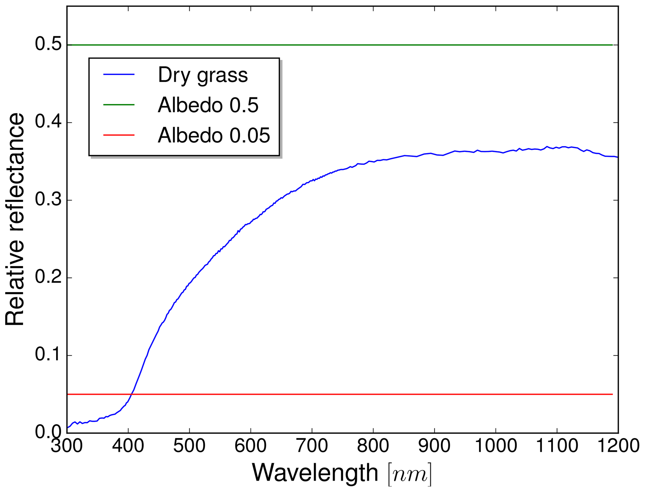
So far, the results above were produced with a spatially and spectrally constant Lambertian surface albedo of 0.05. This does not seem to be a very reasonable assumption since, especially in the near-infrared, albedo over vegetation can reach values of up to 0.5. At the time of the measurements, the environment around the sensor was mainly covered by dried vegetation. The first step to obtain a more realistic albedo setup is to use a wavelength-dependent, spatially constant surface albedo representing the surrounding area. For this task, the dataset AV87-2 from Clark et al. (1993) was used, which refers to dry, long grass, shown in Fig. 8.
The behavior of irradiance over the full spectrum can be seen in Fig. 9. The results are normalized to values obtained with albedo 0.05 and the same settings otherwise. There is an increase in irradiance of about 20 % for the UV wavelengths using the constant surface albedo outside totality (curves for 17:12:00 UTC), which decreases relatively smoothly towards the near-infrared. This is due to the smaller contribution of diffuse irradiance, which is the only part affected by changes in the albedo, in the near-infrared under partial eclipse conditions. If however the wavelength-dependent dry grass albedo from Fig. 8 is applied, there is almost no difference in the irradiance for a partial eclipse over the complete spectrum, compared to the albedo 0.05 surface. The strong increase in the grass' albedo towards longer wavelengths is balanced by the decreased sensitivity of the irradiance in the near-infrared towards changes in the surface reflectance. This is no longer the case as soon as totality starts (curves for 17:20:00 UTC). Setting the albedo from 0.05 to 0.5, the corresponding curve in Fig. 9 reveals a strong wavelength dependence. There are two conspicuous dips around 720 and 940 nm, indicating a coupling between the albedo sensitivity and water vapor absorption. Absorption and more Rayleigh scattering are also the reason for the lower sensitivity in the ultraviolet compared to the near-infrared. In general, an absorbing medium suppresses longer photons paths, which in turn are more likely to interact with the surface. Qualitatively, this behavior is also valid for the grass albedo, however with a smaller effect due to the lower albedo values and increasing curves resulting from the grass albedo increase towards longer wavelengths.
For future implementation of detailed maps of the surrounding, it is necessary to know the influence of different areas in the simulation domain, in order to choose an appropriate resolution of the maps. Therefore, in this second part of the albedo study, several idealized simulations were performed with white disks on an otherwise black surface of albedo 0.0, centered around the observer. All following simulations correspond to 17:19:55 UTC and 555 nm wavelength.
In Fig. 10, fully filled white disks, centered around the observer, were used. The derivative of the relative irradiance with respect to the radius r of the disks expresses the influence of areas located at a distance r. From this, it can be seen that areas at a distance between 20 and 400 km are the reason for most of the observed changes. The albedo of areas more than 600 km away from the observer has almost no effect on the measurements. In our case, this means that the Pacific in the western part of the simulation domain can be neglected. From similar simulations with annuli of different radii, but a fixed area, we see that a unit surface at a greater distance has less influence on the result. However, this is compensated by the growth of the circle area proportional to r2. This leads to a maximal influence for the region around the observer in 100 km distance. From Fig. 10, we conclude that an ideal map should cover the surroundings up to a distance of at least 400 km, possibly at the cost of having a lower resolution.
3.3 Ozone profile
The total column of ozone (TOC) at the measurement site was derived in Bernhard and Petkov (2019) to be 293 DU directly before the eclipse and 294 DU after the end. These values can be compared with measurements of the TOC from the Ozone Monitoring Instrument (OMI) on the Aura satellite, which measured 298 DU TOC the previous day (Veefkind, 2012). In addition, the influence of the vertical distribution of ozone is analyzed using a profile produced with MOZART, the Model for Ozone and Related Chemical Tracers (Emmons et al., 2010). Compared to the midlatitude summer profile, in the MOZART profile 15 DU of ozone were shifted from the lower stratosphere between 10 and 20 km to the altitude range between 20 and 35 km. Both profiles are scaled to 298 DU TOC.
Results can be seen in Fig. 11. There was again no aerosol included in the simulations, but the albedo file for dried grass introduced in Sect. 3.2 was used. Outside the totality at 17:12:00 UTC, a decrease in the total ozone column leads to an increase in irradiance like one would expect for a reduction of an absorbing gas. The sensitivity depends strongly on the ozone cross section, causing changes in irradiance of ±20 % at 304 nm and ±0.5 % around 600 nm (at 304 nm, the optical depth due to ozone is around 2.1, in the Chappuis bands between 400 and 650 nm, it peaks at 0.05).
A change in the ozone distribution has much smaller influence than a change in the total column outside totality in the region of the Chappuis bands. Here the contribution of the direct irradiance is larger than in the ultraviolet, and direct radiation is not affected by the vertical distribution of the absorber but only by the column. In the UV part of the spectrum, the irradiance increases slightly using the profile from MOZART with more ozone in the upper atmosphere. This indicates that most of the photons travel horizontally below 20 km, in accordance with findings in Sect. 3.6. Results inside the totality agree with the results outside in the typical features. Due to the lack of direct radiation, the sensitivity to ozone is generally increased, with changes of up to ±30 % at 304 nm and ±2 % at 600 nm. Since the actual intensities are much smaller, the Monte Carlo simulation is noisier. Without direct solar radiation, it is possible to see the influence of the difference between MOZART and the midlatitude summer profile around 600 nm as well. The influence is comparable to a change in the TOC of 20 DU. This leads to the conclusion that one has to be careful when deriving the total ozone column during totality from irradiance measurements at the surface.

Figure 9Relative spectral irradiance at 17:20:00 (totality) and 17:12:00 UTC (partial eclipse) for different spectral, spatially homogenous distributions of the surface albedo. Values are normalized to the corresponding values obtained at17:12:00 and 17:20:00 UTC with an albedo of 0.05.
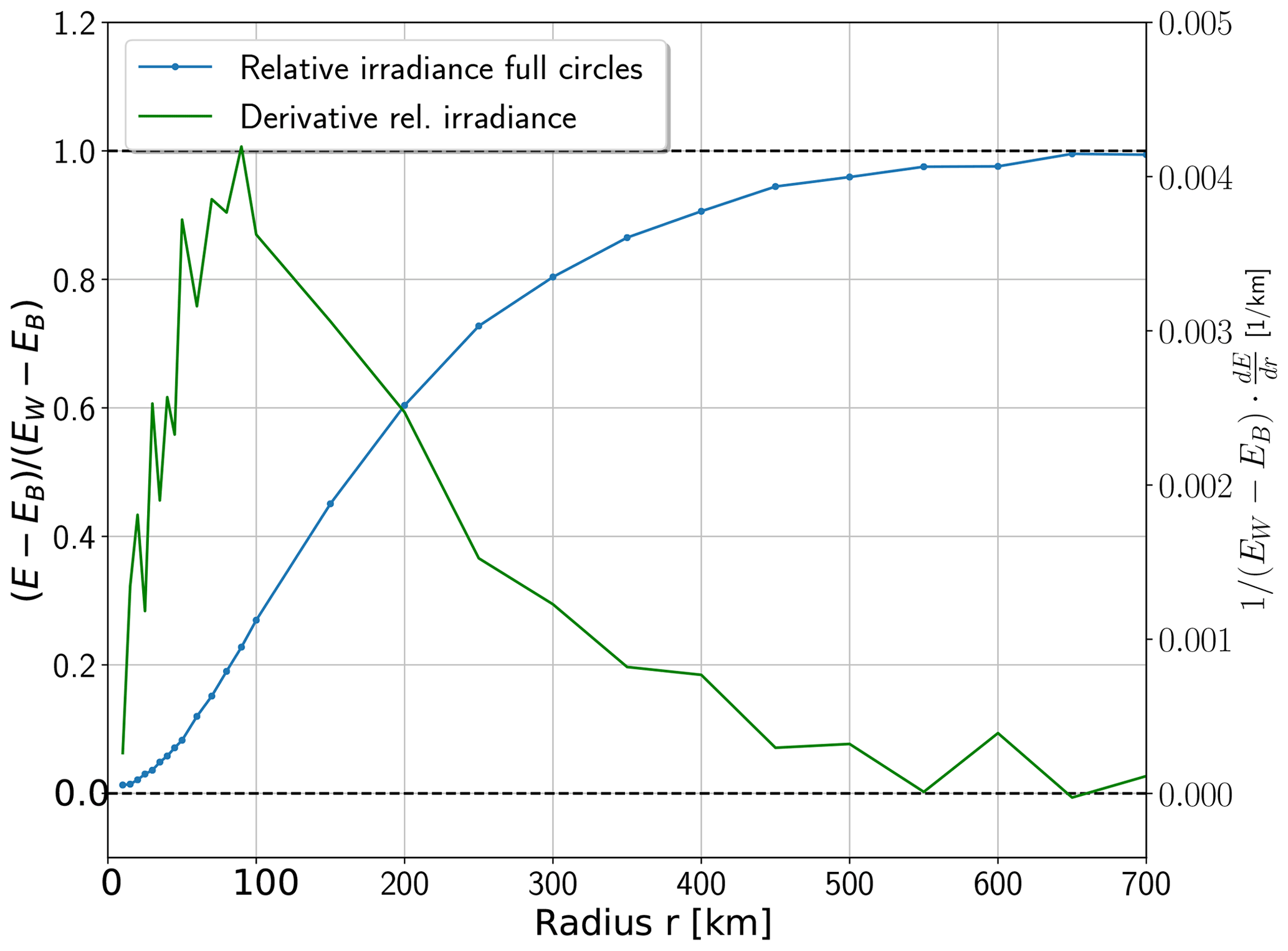
Figure 10Blue line: change in irradiance at 17:19:55 UTC and 555 nm for white, filled circles with different radii centered around the observer. Shown is the difference with the values from a black surface (subscript B), normalized to the difference if the surface is completely white (subscript W). In the latter case, irradiance is increased by a factor of 2.96 compared to the black surface. The green line shows the derivative with respect to the circle radius.
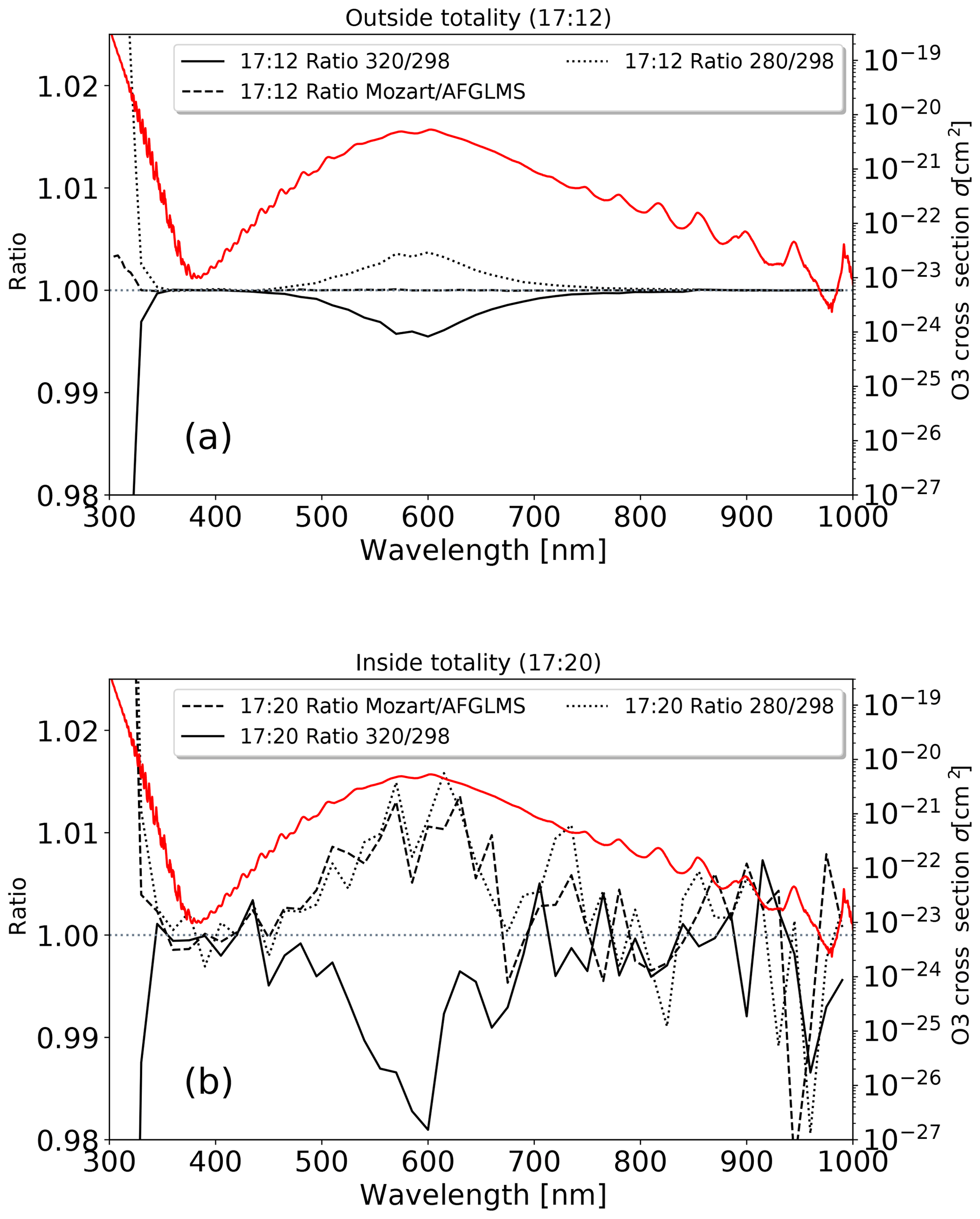
Figure 11Simulated irradiance for a partial eclipse (a) and totality (b) for different wavelengths, normalized to the irradiance at the corresponding wavelength with the midlatitude summer profile scaled to 298 DU TOC. The solid line corresponds to an increase to 320 DU TOC, and the dotted line to a decrease to 280 DU TOC. For the dashed line, the TOC was kept constant to 298 DU TOC, but the midlatitude summer profile was replaced with the one from MOZART. The position of 1.0 is indicated by a coordinate line for better readability. The red curve shows the total ozone absorption cross section and corresponds with values on the right y axis. For 304 nm, changes are ±20 % outside totality and ±30 % inside (not shown).
3.4 Topography
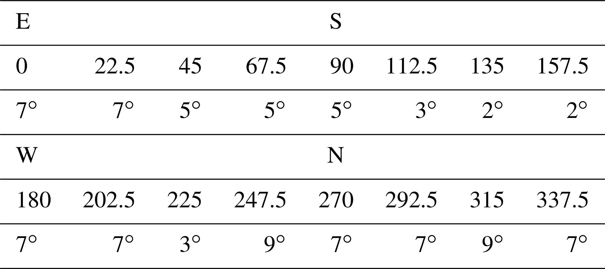
Looking at pictures of solar eclipses, one will see a bright, reddish horizon under a black sky, indicating that mountains likely have an influence and should be included to accurately model the data. The site where Bernhard and Petkov (2019) made the measurements was surrounded by a mountain range. The profile given in Table 2 was estimated from photos. To model the effect on the measured irradiance to the first order, we assume completely black mountains which block all radiance by setting photons coming from angles below θm over the horizon equal to zero. There were three spectral series produced, one without mountains (), one with and one with the mountain profile around the sensor at the measurement site in 2017 shown in Table 2. The last series will be denoted as P2017. The results can be seen in Fig. 12. The curves shares some characteristics with the curves in Fig. 9, where the surface albedo was changed. Eight minutes before the totality, changes of up to 2 % can be observed for the shorter wavelengths. The increase in direct irradiance is the reason for the vanishing differences at longer wavelengths. Observations during totality show reductions in irradiance of up to 60 %. This shows that a disproportionally high amount of radiation comes from the horizon (for isotropically incoming radiance, we would expect only a 3 % reduction in irradiance). As noted earlier, during totality the longer wavelengths are more sensitive towards changes in the surrounding. Again, there are two clearly visible spikes in regions of high absorption, where longer photon paths are suppressed: here, the contribution from photons (which come from higher angle positions over the hilltops) with shorter paths through the atmosphere is enhanced. This agrees with the observation that the sky appears more bluish overhead during an eclipse. Between the 10∘ mountains and the P2017 profile, there are no major differences despite the smaller decrease due to the lower average mountain height in P2017.
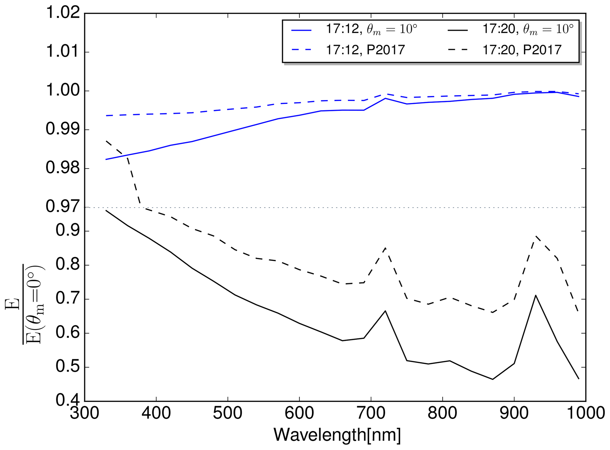
Figure 12Simulated irradiance for different wavelengths and mountain heights, normalized to the irradiance at the corresponding wavelength without mountains (). Note the scale change on the y axis indicated by the dashed, gray line. Blue lines are values outside totality, black lines during totality. Solid lines are for mountains with constant height everywhere around the observer, dashed lines represent the mountain profile P2017 given in Table 2.
Table 2Azimuth angle in degrees (second row) and corresponding height of the mountains over the horizon (third row) in degrees. Values taken from Bernhard and Petkov (2019).
3.5 Aerosol
Another factor which influences direct as well as diffuse irradiance is aerosol. During measurements by Bernhard and Petkov (2019), used for the comparison in Sect. 3.7, several wildfires were burning in the region. Therefore, the authors derived aerosol optical depth (AOD) from measurements of direct spectral irradiance for each channel. At 16:00 and 19:00 UTC, i.e., before the first and after the fourth contact, they fitted Ångström functions of the form to the data. The coefficients for the first measurement are α=1.96 and β=0.057, for the second measurement they obtained α=2.1 and β=0.0394. In our reference simulation, we specify aerosol the same way as the aforementioned authors and similar to Emde and Mayer (2007). This includes an aerosol model of Shettle (1990) with rural-type aerosol in the boundary layer and background aerosol above 2 km. Single scattering albedo was set to 0.95 and the asymmetry parameter to 0.7. This profile is scaled to an AOD described by the Ångström function at 19:00 UTC. Furthermore, the settings from the sections above are applied: dry grass albedo, MOZART ozone profile and realistic mountain profile. In Fig. 13, the blue curve shows the relative change in irradiance during totality if no aerosol were to be present. In the near-infrared the effect is strongest, with signal reductions of up to 60 % despite the generally lower AOD. To obtain an estimate of the uncertainty of the reference simulation, the orange curve was produced with the Ångström parameters from 16:00 UTC. Maximal changes are 10 %. Again, we see the red and near-infrared wavelengths to be more sensitive to the surrounding during totality, which we will explain in the following section.
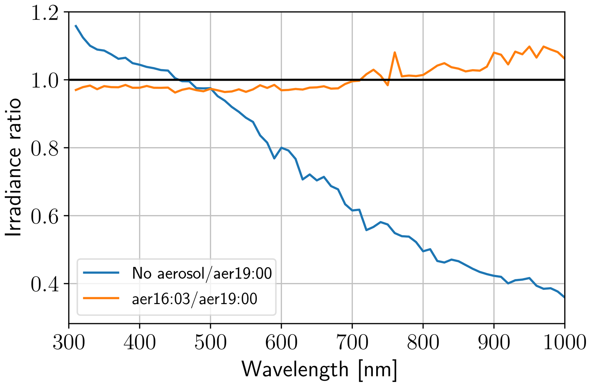
Figure 13Simulated irradiance during totality (17:20:00 UTC) for different wavelengths, relative to irradiance with the Ångström parameters derived at 19:00 UTC. For the blue curve, no aerosol was specified, for the orange curve aerosol was parameterized with the Ångström parameters derived at 16:00 UTC.
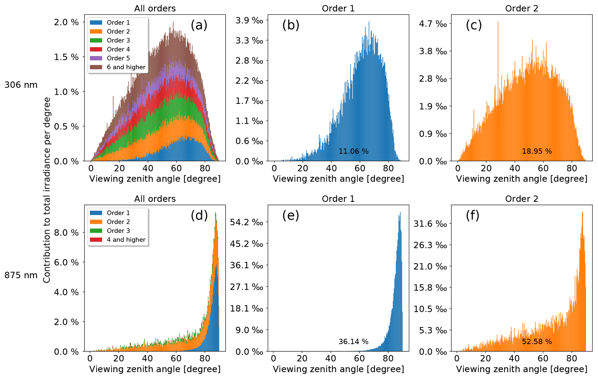
Figure 14Contribution of photons at 306 nm (a–c) and 875 nm (d–f) to the total spectral irradiance per degree incident angle, split into the contributions from different scattering orders. 0∘ corresponds to zenith direction, 90∘ to the horizon. Panel (a) and (d) show the stacked combination of the order-specific plots (b, c, e, f) as histograms. The black percentages represent the total contribution from photons of this scattering order.
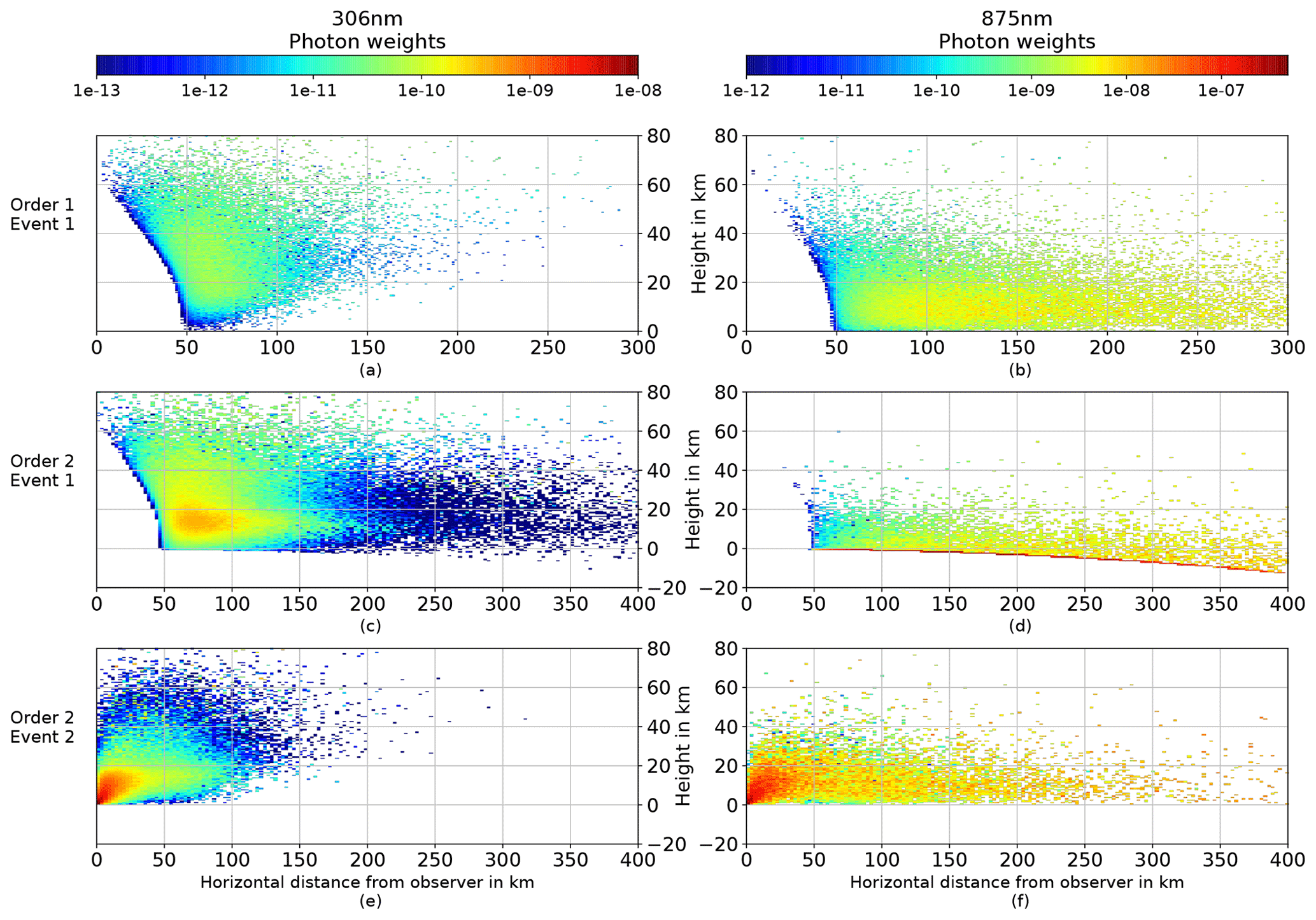
Figure 15Contribution to solar irradiance for photons of different scattering orders and events. “Order” denotes the total number of scatterings, “Event” numbers the scattering event on a path from TOA to the sensor. The horizontal axis denotes the horizontal distance from the observer, the vertical axis the distance from the observer in zenith direction. Contributions are summed radially. Due to the usage of cartesian coordinates in combination with the curvature of the Earth, negative scattering heights are possible.
3.6 Photon paths
Many of the effects analyzed in the sections above can be qualitatively understood by looking at the photon paths through the atmosphere. It is important to include the Monte Carlo weighting of the photons, which expresses the effect of the eclipse, the air's optical thickness and scattering direction probabilities (for details about the weights, we refer the reader to Marshak and Davis, 2005). To simplify the geometry, simulations are done for an observing point directly in the shadow center at 17:20:00 UTC and without any mountains obstructing the horizon. Otherwise, the settings are the same as before; specifically, the dry grass albedo from Sect. 3.2 and the MOZART ozone profile from Sect. 3.3 are used. In Fig. 14, the elevation angle under which the photons arrive at the observer is shown for photons of different scattering order. The results include a cosine weighting to account for the effective area of the sensor. At 306 nm, most of the measured irradiance comes from photons of the order of 2 (20 %), in contrast with diffuse irradiance under non-eclipse conditions, where single scattered photons make up almost half of the result (not shown). Orders higher than 2 have monotonically decreasing importance, with a 1 % contribution from the order of 10 (non-eclipse: 0.2 %). The higher-order angle distributions approximately follow the sin θ⋅cos θ distribution one would expect for isotropically incoming photons, whereas photons of the order of 1 show a distortion towards the horizon. For order 2 and higher, sometimes single photons exhibit an exceptionally high weight, showing up as strong peaks in the histogram. These photons enter the atmosphere with a high initial weight due to the large distance to the umbra (up to 800 km away from the observer) and then travel horizontally 60 km above the surface until they are vertically scattered down to the observer. At 875 nm, most of the contribution comes from doubly scattered photons as well. However, photons with large incident angles are much more important than at 306 nm, as well as for diffuse irradiance under normal conditions at 875 nm. This explains the red horizon during an eclipse and the influence of the topography (Sect. 3.4). The underlying reason can be seen in Fig. 15, which shows the spatial density of scattering events for photons of the order of 1 and 2. For the first scattering event, the lunar shadow creates a forbidden volume with the shape of a cylinder in the 3-D atmosphere, inclined towards the Sun. Longwave photons have their last scattering event on average at a greater distance than shortwave photons (see Fig. 15a, e and b, f) and therefore larger incident angles. The higher reflectivity of the surface at 875 nm adds to this effect. Actually, most of the multiply scattered photons at longer wavelengths have contact with the Earth's surface, which can be clearly seen in Fig. 15d, and this explains the surface influence found in Sect. 3.2. Comparing the maximum in Fig. 15c to the one in Fig. 15e, the main photon paths likely contain a 50–70 km horizontal part below 20 km. This is in agreement with the findings in Sect. 3.3 that the MOZART profile, with more ozone above 20 km, leads to increased irradiance during totality.
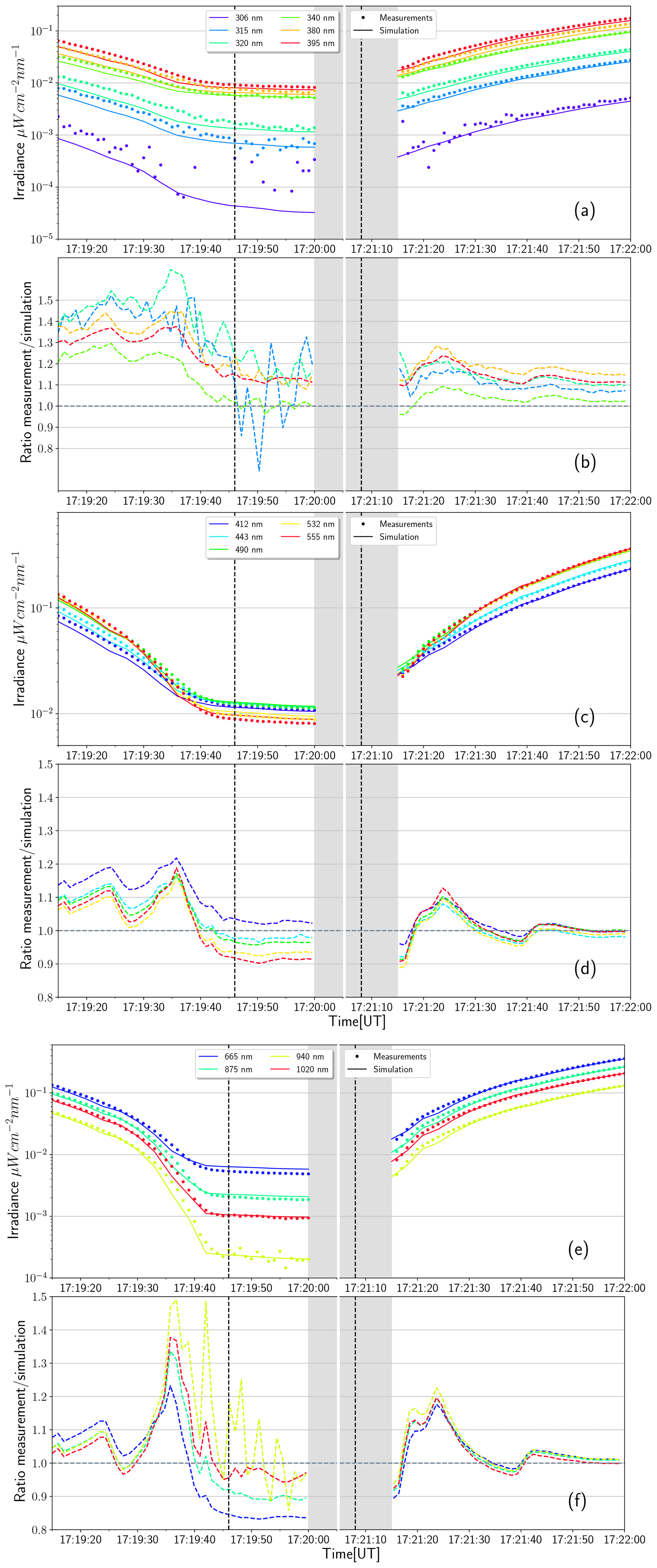
Figure 16Comparison of simulation and measurements for wavelengths from 306 to 1020 nm. Panel (a) shows simulated (solid line) and measured (dotted line) irradiance for wavelengths in the range from 300 to 400 nm. Panel (b) shows the measurements divided by the simulation values (dashed line). The x axis is discontinuous and does not show the period between 17:20:05 and 17:21:05 UTC because the shadow band swiped over the sensor between 17:20:00 and 17:21:10 UTC (gray shading). The vertical, dashed lines show the theoretical start and end of totality. (c, d) Same as (a) and (b), but for wavelengths from 400 to 600 nm. (e, f) Same as (a) and (b), but for wavelengths from 600 to 1020 nm.
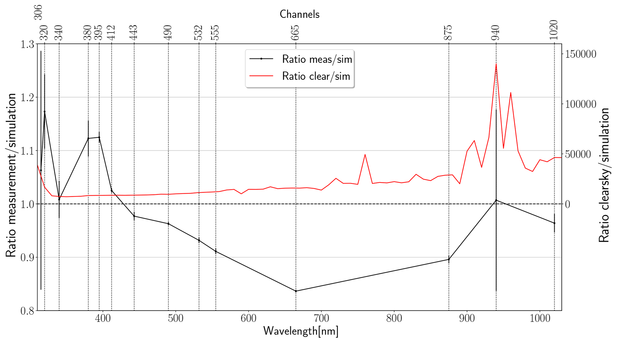
Figure 17Spectral irradiance during totality (17:20 UTC). The black curve shows the deviation of the measurements from the totality simulations, averaged over the 12 data points during totality (17:19:48–17:20:00 UTC). The error bars indicate 1σ deviation of the original values from the mean. Vertical lines indicate the position of the measurement channels. The red curve shows the ratio of the simulated clear-sky irradiance (i.e., without lunar occultation) to simulated totality irradiance at 17:20:00 UTC.
3.7 Comparison with measurements
Measurements of global spectral irradiance at different wavelengths were taken by Bernhard and Petkov (2019). Details of the measurement conditions and the calibration process can be found there; the following provides a short summary. The instrument was placed on a field near the Crooked River, which flows through Smith Rock State Park and is surrounded by dry grass. In the west and northeast, mountains obstruct the horizon by up to 12∘. The sky on this morning was almost clear with only a few clouds near the horizon. There were several wildfires in the region burning at the measurement time. On the day of the measurement however, the wind direction changed in favor of a decrease in aerosol loading. The instrument used was a GUVis-3511 multi-channel filter radiometer constructed by Biospherical Instruments Inc. The sensor was placed approximately 2 m above the ground. It was equipped with a computer-controlled shadow band, allowing calculation of direct and global spectral irradiance from the instruments measurements at 306, 315, 320, 340, 380, 395, 412, 443, 490, 532, 555, 665, 875, 940 and 1020 nm with a spectral resolution of 1 nm.
When comparing the measurements around the totality with results from the model, we included the most realistic settings; i.e., we used the spectral dependence of dry grass for the albedo, the ozone profile from MOZART, the mountain profile from Table 2 and the reference aerosol settings from Sect. 3.5. The column of precipitable water was set to 11 kg m−2 by scaling the midlatitude summer profile. The value was chosen to achieve best agreement between the measurements from 19:00 to 20:00 UTC and the 940 nm channel, which is strongly influenced by water vapor. This is 20 % less than the value of 13.85 kg m−2 given by the ERA-Interim global reanalysis at the place and time of the eclipse (Dee et al., 2011).
In a first step, these settings are applied to the 1-D radiative transfer solver “disort”, which is part of libRadtran as well. At 19:00 UTC (20 min after the fourth contact), the results agree with the measurements to better than 5 % at each wavelength. This deviation might be caused by uncertainties in the measurements or in the parametrization of the atmospheric state, e.g., that of the aerosol loading. To correct the simulation for these errors, which have nothing to do with the eclipse, the simulation values were multiplied by the average deviation between 19:00 and 20:00 UTC for each wavelength.
The comparison of the results of the 3-D calculations and the measurements from 17:18 until 17:23 UTC can be seen in Fig. 16. In each case, the corrected simulations and the measured values are shown in panel (a) of the figure. In panel (b), the ratio of observation and simulation is shown. From 17:20:00 until 17:21:15 UTC, the shadow band swept over the sensor, indicated by the gray gap in the time series. In all three domains, the deviations are increased directly before and after the totality, where the temporal gradient of irradiance is very large. Here, the measurements exceed the simulation up to 60 % (at 320 nm), giving information about temporal uncertainties which are intensified in these regions. Because the peaks indicate lower simulation results both before and after the totality, the deviation is likely not a temporal shift in one direction, but a difference of 1–2 s between the actual duration of totality and the period assumed by the simulation. The potential reasons are manifold; e.g., small errors in the lunar disk radius or the Moon's deviation from a perfect sphere could change the shadow's size easily and therefore affect the totality time.
The spectral ratio of measurement and simulation during totality is also shown in Fig. , together with the ratio of clear-sky calculations (i.e., without lunar occultation) to totality simulations. Generally, absorbing wavelengths are attenuated more compared to clear-sky conditions, with ranges from 7170 at 350 nm to 140 000 at 940 nm. These values agree with the ones obtained by Bernhard and Petkov (2019).
Looking at the wavelength domains separately, the best results are achieved between 400 and 600 nm (Fig. 16). Agreement outside the totality is within 3 %; during totality the values agree within 10 %. There are several reasons why these wavelengths are easier to simulate and measure. Their clear-sky intensities exceed the other domains by at least 50 %; additionally, there are only few absorbing trace gases. However, there seems to be a systematic deviation towards longer wavelengths, being simulated too high during totality (compare to the downward trend in the black line in Fig. between 400 and 700 nm). From the sensitivity analysis, one could attribute this observation to the ozone profile, which affects the 500–700 nm range only during totality. Compared to Fig. 11, a change in 10 % for 555 nm might be possible, but would certainly induce changes by more than 10 % in the ultraviolet as a consequence.
For 600–1020 nm (Fig. 16), the results are comparable, with somewhat more fluctuations due to the lower solar intensities. The 1020 nm curve shows nearly perfect agreement regarding the intensities, but the temporal uncertainty is one of the highest for all channels. 665 nm shows better temporal agreement, but continues the trend of higher simulation results at totality also described for the 400–600 nm domain. As mentioned, the 940 nm channel depends highly on the water vapor concentration in the atmosphere, a quantity with typically large fluctuations in time and space. Nevertheless, the agreement outside the totality is as good as for the other wavelengths in this domain. Of course, one has to remember that the total water vapor column was scaled to fit this channel. Inside the totality, there is too much noise in the 940 nm measurement signal to make a precise statement, although the mean value fits the simulation well.
Between 300 and 400 nm (Fig. 16), the discrepancy between measurements and simulations is larger compared to the other wavelength domains. Since the intensities are comparably low here, the sensor operates close to its detection limit for 306 and 315 nm during totality, which is clearly visible in the large fluctuations. The ratio for 306 nm is not plotted therefore. Outside the totality, all wavelengths are simulated too low. This is likely not attributable to ozone, which affects mostly the wavelengths below 350 nm. It is interesting that the simulation agrees much better with the measurement at 412 nm than at 395 nm. These wavelengths are close to a critical region in the limb darkening parametrizations, where hydrogen can become fully ionized from the second shell (364.66 nm). Exactly the same behavior can be seen in Bernhard and Petkov (2019) (see their Fig. 9) using 1-D simulations, even with different limb darkening parametrizations. In addition, 395 nm is right between the strong Ca+ Fraunhofer lines at 393 and 396.5 nm. As a consequence, there is some uncertainty in the measurements from converting the measurements with the GUV's 10 nm wide filters to spectral irradiance at 1 nm resolution. This effect could contribute to the larger difference at 395 compared to 412 nm.
In this study, the three-dimensional radiative transfer model MYSTIC was used to simulate irradiance at the ground during a total eclipse. The celestial part includes the precise geometry of the Sun and Moon, as well as parametrizations for the limb darkening of the Sun. The atmosphere contains realistic gas profiles, a surface with spectrally dependent reflection and a simple topography model. The approach relies only on the time-resolved position of the Sun and Moon in space; all further properties like the position, orientation and the elliptical shape of the lunar shadow are derived from this information. The agreement with the observations illustrate the high accuracy of the umbra calculations using the data from JPL Horizons. There are no restrictions on the observer; e.g., it could be outside of the shadow's center line, as was the case in this study, or even outside of the totality path.
The simulation was applied to the total solar eclipse of 21 August 2017, and the effects of the surface reflectance, ozone profile and the topography were analyzed. In general, we found that the eclipse enhances the sensitivity of global irradiance towards changes in the albedo and topography, which is in large part explained by the absence of direct radiation and the stronger sensitivity of diffuse irradiance to these parameters. Compared to diffuse irradiance for near-infrared wavelengths under non-eclipse conditions, more radiation comes from the horizon. The importance of single scattered photons is generally reduced. Higher orders are able to interact with the surface before reaching the observer, which is why the surface reflectance may cause changes up to 200 % in the measured irradiance for near-infrared wavelengths (completely absorbing versus reflecting surface). Depending on the wavelength, photons from distances of up to 400 km contribute to the result. Due to the long horizontal photon paths, even for ultraviolet wavelengths, not only the total column, but also the vertical distribution of ozone becomes important. Therefore, derivations of the total amount of ozone during totality by comparing surface irradiance measurements at different wavelengths might be misleading. In general, these features of a solar eclipse pose a challenge for models and the assumptions used here are only first-order corrections.
The comparison with measurements reveals that solar irradiance over the course of the eclipse can be modeled with high accuracy, considering that solar irradiance drops by 4–5 orders of magnitude during an eclipse. Showing less than 10 % deviation during the totality at most wavelengths, this also represents a validation of the 3-D radiative transfer model MYSTIC as the core of our model.
Measurements of the GUVis-3511 have been published in the supplement of Bernhard and Petkov (2019) and are available at https://doi.org/10.5194/acp-19-4703-2019-supplement. The radiative transfer models are available open-source via http://libradtran.org (last acess: 20 December 2019). The values of our key results in Figs. 16 and 17 are available in the Supplement. We are open to applying the model to any future eclipse settings. Please do not hesitate to get in touch if you are interested.
The supplement related to this article is available online at: https://doi.org/10.5194/acp-20-1961-2020-supplement.
BM and CE developed MYSTIC and the general setup to simulate a solar eclipse. PO further adapted the setup, performed the model analysis and wrote the paper. GB designed and executed the measurements.
Germar Bernhard is employed by Biospherical Instruments Inc., which is also the manufacturer of the GUVis-3511 radiometer used for the measurements.
We thank the three anonymous reviewers for their commitment and their comments that improved the publication.
This paper was edited by Stelios Kazadzis and reviewed by three anonymous referees.
Anderson, G., Clough, S., Kneizys, F., Chetwynd, J., and Shettle, E.: AFGL Atmospheric Constituent Profiles (0–120km), Tech. Rep. AFGL-TR-86-0110. Tech. rep. Hanscom AFB, MA 01731: Air Force Geophysics Laboratory, 1986. a
Aplin, K. L., Scott, C. J., and Gray, S. L.: Atmospheric changes from solar eclipses, Philos. T. Roy. Soc. A, 374, 20150217, https://doi.org/10.1098/rsta.2015.0217, 2016. a
Archinal, B. A., Acton, C. H., A'Hearn, M. F., Conrad, A., Consolmagno, G. J., Duxbury, T., Hestroffer, D., Hilton, J. L., Kirk, R. L., Klioner, S. A., McCarthy, D., Meech, K., Oberst, J., Ping, J., Seidelmann, P. K., Tholen, D. J., Thomas, P. C., and Williams, I. P.: Report of the IAU Working Group on Cartographic Coordinates and Rotational Elements: 2015, Celest. Mech. Dyn. Astr., 130, issn 1572-9478, https://doi.org/10.1007/s10569-017-9805-5, 2018. a
Bernhard, G. and Petkov, B.: Measurements of spectral irradiance during the solar eclipse of 21 August 2017: reassessment of the effect of solar limb darkening and of changes in total ozone, Atmos. Chem. Phys., 19, 4703–4719, https://doi.org/10.5194/acp-19-4703-2019, 2019. a, b, c, d, e, f, g, h, i, j, k, l
Bernhard, G., Booth, C., and Ehramjian, J.: Version 2 data of the National Science Foundation's Ultraviolet Radiation Monitoring Network, Sol. Energy, 74, 423–453, 2004. a
Calamas, D. M., Nutter, C., and Guajardo, D. N.: Effect of 21 August 2017 solar eclipse on surface-level irradiance and ambient temperature, International Journal of Energy and Environmental Engineering, 10.2, 147–156, https://doi.org/10.1007/s40095-018-0290-8, 2018. a
Clark, R. N., Swayze, G. A., Gallagher, A. J., King, T. V., and Calvin, W. M.: The U. S. Geological Survey, Digital Spectral Library: Version 1 (0.2 to 3.0um), https://doi.org/10.3133/ofr93592, 1993. a, b
Dee, D. P., Uppala, S. M., Simmons, A. J., Berrisford, P., Poli, P., Kobayashi, S., Andrae, U., Balmaseda, M. A., Balsamo, G., Bauer, P., Bechtold, P., Beljaars, A. C. M., van de Berg, L., Bidlot, J., Bormann, N., Delsol, C., Dragani, R., Fuentes, M., Geer, A. J., Haimberger, L., Healy, S. B., Hersbach, H., Hólm, E. V., Isaksen, L., Kallberg, P., Koehler, M., Matricardi, M., McNally, A. P., MongeSanz, B. M., Morcrette, J.-J., Park, B.-K., Peubey, C., de Rosnay, P., Tavolato, C., Thépaut, J.-N., and Vitart, F.: The ERAInterim reanalysis: configuration and performance of the data assimilation system, Q. J. Roy. Meteor. Soc., 137, 553–597, https://doi.org/10.1002/qj.828, 2011. a
Emde, C. and Mayer, B.: Simulation of solar radiation during a total eclipse: a challenge for radiative transfer, Atmos. Chem. Phys., 7, 2259–2270, https://doi.org/10.5194/acp-7-2259-2007, 2007. a, b, c, d, e, f, g, h, i
Emde, C., Buras-Schnell, R., Kylling, A., Mayer, B., Gasteiger, J., Hamann, U., Kylling, J., Richter, B., Pause, C., Dowling, T., and Bugliaro, L.: The libRadtran software package for radiative transfer calculations (version 2.0.1), Geosci. Model Dev., 9, 1647–1672, https://doi.org/10.5194/gmd-9-1647-2016, 2016. a
Emmons, L. K., Walters, S., Hess, P. G., Lamarque, J.-F., Pfister, G. G., Fillmore, D., Granier, C., Guenther, A., Kinnison, D., Laepple, T., Orlando, J., Tie, X., Tyndall, G., Wiedinmyer, C., Baughcum, S. L., and Kloster, S.: Description and evaluation of the Model for Ozone and Related chemical Tracers, version 4 (MOZART-4), Geosci. Model Dev., 3, 43–67, https://doi.org/10.5194/gmd-3-43-2010, 2010. a
Espenak, F.: EclipseWise.com, available at: http://www.eclipsewise.com/solar/SEgmap/2001-2100/SE2017Aug21Tgmap.html (last access: 7 February 2020), 2018. a
Giorgini, J. D., Yeomans, D. K., Chamberlin, A. B., Chodas, P. W., Jacobson, R. A., Keesey, M. S., Lieske, J. H., Ostro, S. J., Standish, E. M., and Wimberly, R. N.: JPL's On-Line Solar System Data Service, in: AAS/Division for Planetary Sciences Meeting Abstracts #28, vol. 28 of Bulletin of the American Astronomical Society, p. 1158, 1996. a
Groebner, J., Kazadzis, S., Kouremeti, N., Doppler, L., Tagirov, R., and Shapiro, A. I.: Spectral solar variations during the eclipse of March 20th, 2015 at two European sites, in: AIP Conference Proceedings, 1810, 080008, https://doi.org/10.1063/1.4975539, 2017. a
Gueymard, C.: The sun's total and spectral irradiance for solar energy applications and solar radiation models, J. Geophys. Res., 109, 423–453, https://doi.org/10.1029/2004JD004937, 2004. a
Iqbal, M.: An Introduction to Solar Radiation, Academic Press, Don Mills, Ontario, Canada, 1983. a
Kazantzidis, A., Bais, A. F., Emde, C., Kazadzis, S., and Zerefos, C. S.: Attenuation of global ultraviolet and visible irradiance over Greece during the total solar eclipse of 29 March 2006, Atmos. Chem. Phys., 7, 5959–5969, https://doi.org/10.5194/acp-7-5959-2007, 2007. a, b, c
Koepke, P., Reuder, J., and Schween, J.: Spectral variation of the solar radiation during an eclipse, Meteorol. Z., 10, 179–186, https://doi.org/10.1127/0941-2948/2001/0010-0179, 2001. a, b
Marshak, A. and Davis, A.: 3D Radiative Transfer in Cloudy Atmospheres, Springer-Verlag, Berlin, Heidelberg, 2005. a, b
Mayer, B.: Radiative transfer in the cloudy atmosphere, Eur. Physical J. Conf., 1, 75–99, https://doi.org/10.1140/epjconf/e2009-00912-1, 2009. a, b
Mayer, B. and Kylling, A.: Technical note: The libRadtran software package for radiative transfer calculations – description and examples of use, Atmos. Chem. Phys., 5, 1855–1877, https://doi.org/10.5194/acp-5-1855-2005, 2005. a
Pierce, A. K. and Slaughter, C. D.: Solar limb darkening, Sol. Phys., 51, 25–41, https://doi.org/10.1007/bf00240442, 1977. a, b, c, d
Pierce, A. K., Slaughter, C. D., and Weinberger, D.: Solar limb darkening in the interval 7404-24 018, II, Sol. Phys., 52, 179–189, https://doi.org/10.1007/bf00935800, 1977. a, b, c, d
Shettle, E.: Models of aerosols, clouds, and precipitation for atmospheric propagation studies, AGARD Conf. Proce., in: Proc. AGARD, Atmos. Propag. UV, Visible, IR, MM-Wave Region Rel. Syst. Aspects - 1, 1–13, 1990. a
Veefkind, P.: OMI/Aura Ozone (O3) DOAS Total Column Daily L3 Global 0.25deg Lat/Lon Grid, NASA Goddard Earth Sciences Data and Information Services Center, https://doi.org/10.5067/aura/omi/data3005, 2012. a
Waldmeier, M.: Ergebnisse und Probleme der Sonnenforschung, vol. 2, Akademische Verlagsgesellschaft Geest&Portig K.G., 1955. a
Zerefos, C. S., Balis, D. S., Meleti, C., Bais, A. F., Tourpali, K., Kourtidis, K., Vanicek, K., Cappellani, F., Kaminski, U., Colombo, T., Stuebi, R., Manea, L., Formenti, P., and Andreae, M. O.: Changes in surface solar UV irradiances and total ozone during the solar eclipse of August 11, 1999, J. Geophys. Res.-Atmos., 105, 26463–26473, https://doi.org/10.1029/2000jd900412, 2000. a