A mid-latitude cyclone was centred off the southern tip of Greenland on 2 February 2012. The warm front extended eastwards across Iceland towards Scandinavia, whilst the cold front extended roughly north–south over the Atlantic Ocean a few hundred kilometres west of Ireland. The broad warm sector covered the north-west of the UK, with high pressure to the south and east. Figure 1 shows a 10.8 µm infrared satellite image of the North Atlantic region from the AVHRR (Advanced Very High Resolution Radiometer) for the north-eastern Atlantic, including the western UK and Ireland, Iceland, and part of Greenland. Extensive layer cloud was observed within the warm sector. Close to the low-pressure centre, west of 10^∘ W, the cloud top temperature was colder than −50 ^∘C, and to the south-east the cloud top temperature was between −18 and −29 ^∘C, as estimated using Met Office products derived from MSG (Meteosat Second Generation) and NWP output. Discussion regarding this technique can be found in Hamann et al. (2014).

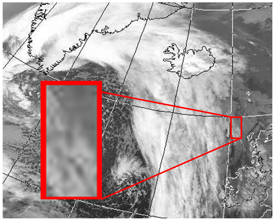
Figure 1Infrared satellite imagery (10.8 µm) from the AVHRR at 14:40 UTC, 2 February 2012. Layer cloud associated with the warm sector is visible to the west of the UK. The red box indicates the location of the airborne sampling.

In situ data were collected from the FAAM BAe146 Atmospheric Research Aircraft (FAAM, 2017) from single-layer mixed-phase altocumulus clouds within the warm sector of a mid-latitude cyclone, sampled on 2 February 2012 (FAAM Flight B674). Data collection began in the afternoon (16:00 UTC) with the end of the measurement period being flown in twilight conditions (19:00 UTC). The choice of flight track was restricted by air traffic considerations and so it was impossible to advect with the cloud in a Lagrangian sampling strategy. Fortunately the north–south flight track was closely aligned to the direction of the mean wind, which was predominantly from the south and ranged in strength from 6 m s⁻¹ at the southern end of the flight track to 8 m s⁻¹ in the north. There was some degree of wind shear above the cloud-containing layer, with mean wind direction being close to northwesterly. This shear may have resulted in production of turbulence in the layer below.

An optically opaque liquid cloud with cellular structure and an areal coverage of between 6 and 7 Oktas was observed upon arrival in the area, along with ice virga which extended below the liquid cloud base, as shown in the photograph in Fig. 2. Visual observation from the flight deck and real-time inspection of in situ data revealed that the cloud-containing layer was capped by a weak temperature inversion (≈1 K), below which sat the liquid cloud layer. Liquid cloud top sloped from 5800 m ($T=-\mathrm{31}$ ^∘C) at the southern extent of the sampling region to 5400 m ($T=-\mathrm{27}$ ^∘C) at the northern end. Constant-altitude flight segments interspersed with slant profiles were flown between 4500 and 7500 m. The slant profiles indicated a pseudo-adiabatic liquid water structure with larger liquid water content towards cloud tops, similar to observations by Korolev et al. (2007).

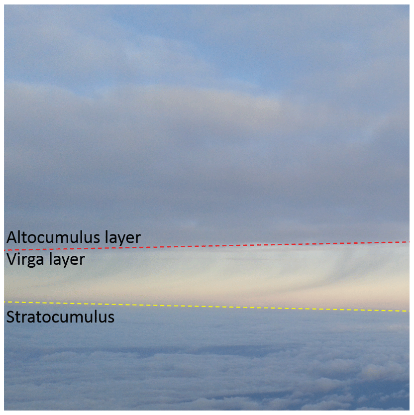
Figure 2Photograph of the altocumulus layer from underneath the liquid layer, within the precipitating ice virga layer, taken on arrival in the operating area at 16:17 UTC, 2 February 2012. The broken cellular structure of the liquid altocumulus layer cloud is visible above the dashed red line. Ice virga can be seen below the liquid cloud, advected with the mean wind from right to left (south to north), between the dashed red and yellow lines. Boundary layer stratocumulus cloud is visible below the dashed yellow line. Photo: S. Abel.

Download

The BAe146 carries a scientific payload capable of measuring meteorological and thermodynamic conditions and bulk and microphysical cloud properties, described in part by Mirza et al. (2016) and Allen et al. (2014).

Data were selected from times when the aircraft was flying a constant heading using the limits for rate of change of heading and roll in Table 1. Slant profiles were flown at a vertical rate of change of 5 m s⁻¹, whereas a straight and level run (SLR) had a rate of change of altitude less than 0.5 m s⁻¹. During sampling the aircraft typically had a nominal indicated airspeed (IAS) of 210 kn, approximately 140 m s⁻¹ in the mid-troposphere.

Table 1Parameters and limits used in determining when aircraft is in a straight and level run (SLR) and a slant profile (Pro).

Download Print Version | Download XLSX

Turbulent wind components were sampled in three dimensions at 32 Hz using a five-port turbulence probe located on the nose of the aircraft (e.g. Petersen and Renfrew, 2009). No problems due to icing of the turbulence probe pressure ports were observed during data collection.

Temperature measurements were recorded at 32 Hz by a non-de-iced Goodrich Type 102 platinum resistance thermometer and reported at 1 Hz. There was no evidence of contamination on this sensor housing due to the presence of condensed liquid water when compared against the deiced sensor. Humidity data were provided at 0.4 Hz by a near-infrared tunable diode laser (TDL) absolute humidity spectrometer, a WVSS2 (Water Vapour Sensing System Mk. 2) fitted to a flush-mounted inlet (Vance et al., 2014), allowing computation of dew point temperature and water vapour mixing ratio, q_v.

Bulk LWC measurements were made using a Nevzorov hot-wire probe (Abel et al., 2014). Data from the Nevzorov total water sensor (LWC + IWC) were also interrogated to identify regions of cloud-free air that would permit use of out-of-cloud aerosol particle observations; for details, see Appendix A. A Lyman-alpha total water content (q_t) instrument (Brown and Francis, 1995) was employed to estimate total water mixing ratio, q_t=q_v + LWC + IWC.

Liquid cloud particle size and number concentration were measured using a CDP (cloud droplet probe) with anti-shatter tips fitted (Lance et al., 2010). The performance of the probe was monitored using glass spheres of known diameter following the method presented in Rosenberg et al. (2012). The CDP was calibrated prior to the field campaign, and additional glass bead checks were routinely performed throughout in order to ensure that there was no drift in performance. The integrated LWC from CDP compared well with that measured by the Nevzorov hot-wire probe (Pearson correlation coefficient = 0.98), with slight over-reading at larger sizes, where the calibration is more uncertain. Ice particle number concentrations were measured by two optical array probes (OAPs), i.e. the Cloud Imaging Probes (CIPs), with CIP15 for diameters 30 µm $\le D\le \mathrm{960}$ µm in 15 µm increments and CIP100 (100 µm $\le D\le \mathrm{6.2}$ mm) in 100 µm increments (Cotton et al., 2013). Data were processed using the SODA2 package (System for OAP Data Analysis version 2; Bansemar, 2016) from NCAR (National Centre for Atmospheric Research). Maximum observed ice crystal diameters were often less than 1 mm in this study and so the impact of shattered ice fragments on microphysical measurements is expected to be low, and careful inspection of particle imagery from the CIP probes supports this. Additionally, an algorithm to remove shattering artefacts based on the inter-arrival times of particles was applied. Imagery of cloud particles was provided by a Cloud Particle Imager (CPI) probe (Connolly et al., 2007). Cloud fraction was computed for both liquid (CDP) and ice particle (CIP15) observations by examination of the ratio of 1 s periods with and without cloud particles in a given altitude range. Full details are given in Appendix A.

Aerosol particle number concentration and size were sampled in the nominal size range 0.1 µm $\le D\le \mathrm{3.0}$ µm with a Passive Cavity Aerosol Spectrometer Probe (PCASP) (Knollenberg, 1970), which was calibrated at FAAM using the method of Rosenberg et al. (2012). Full details of the data processing are given in Appendix A.

In the absence of an ice nucleus counter (INC) an assessment of the ice-nucleating particle (INP) concentration was made by measuring the number concentration of aerosols with diameter, D≥0.5 µm and applying empirically based temperature-dependent parameterisations from DeMott et al. (2015) for general aerosol particles and Tobo et al. (2013) for forest emissions of INP.

When flying above cloud the cloud top height (CTH) was measured using data from a downward facing Leosphere ALS450 backscatter lidar, using an integration time of 2 s and vertical resolution of 1.5 m (Allen et al., 2014; Osborne et al., 2014). During a preliminary measurement leg, flying above cloud, it was observed that the cloud top height sloped along the flight track. This was coupled with the fact that air traffic restrictions prevented Lagrangian cloud sampling in the horizontal. It was therefore decided to develop an air-relative coordinate system, anchored to cloud top height (or inversion altitude) in the vertical and neglecting the horizontal dimension. Cloud top was constrained at an isentropic surface by a thermodynamic inversion which was crossed nine times between 17:10 and 17:35 UTC and a further six times later in the measurement period, between 18:25 and 18:40 UTC, in the southern half of the region. Many of these profiles contained cloud. The cloud layer below the inversion was identified from measurements of total water mixing ratio. The cloud layer was measured at q_t=0.725 g m⁻³, as compared to the free troposphere above, where q_t=0.45 g m⁻³. Within the cloud layer wind speed was greater in the north, and a linear fit was produced to give wind speed as a function of latitude. This allowed for an estimate of the air-relative horizontal coordinate and hence two new vertical coordinates: the vertical position of the aircraft relative to the spatially and temporally varying (i) CTH, Δz_(CTH), and (ii) the inversion (top) altitude, Δz_(inv.). Estimated time series of both inversion and cloud top altitude using these spot measurements were generated by interpolating in space and time throughout the measurement period.

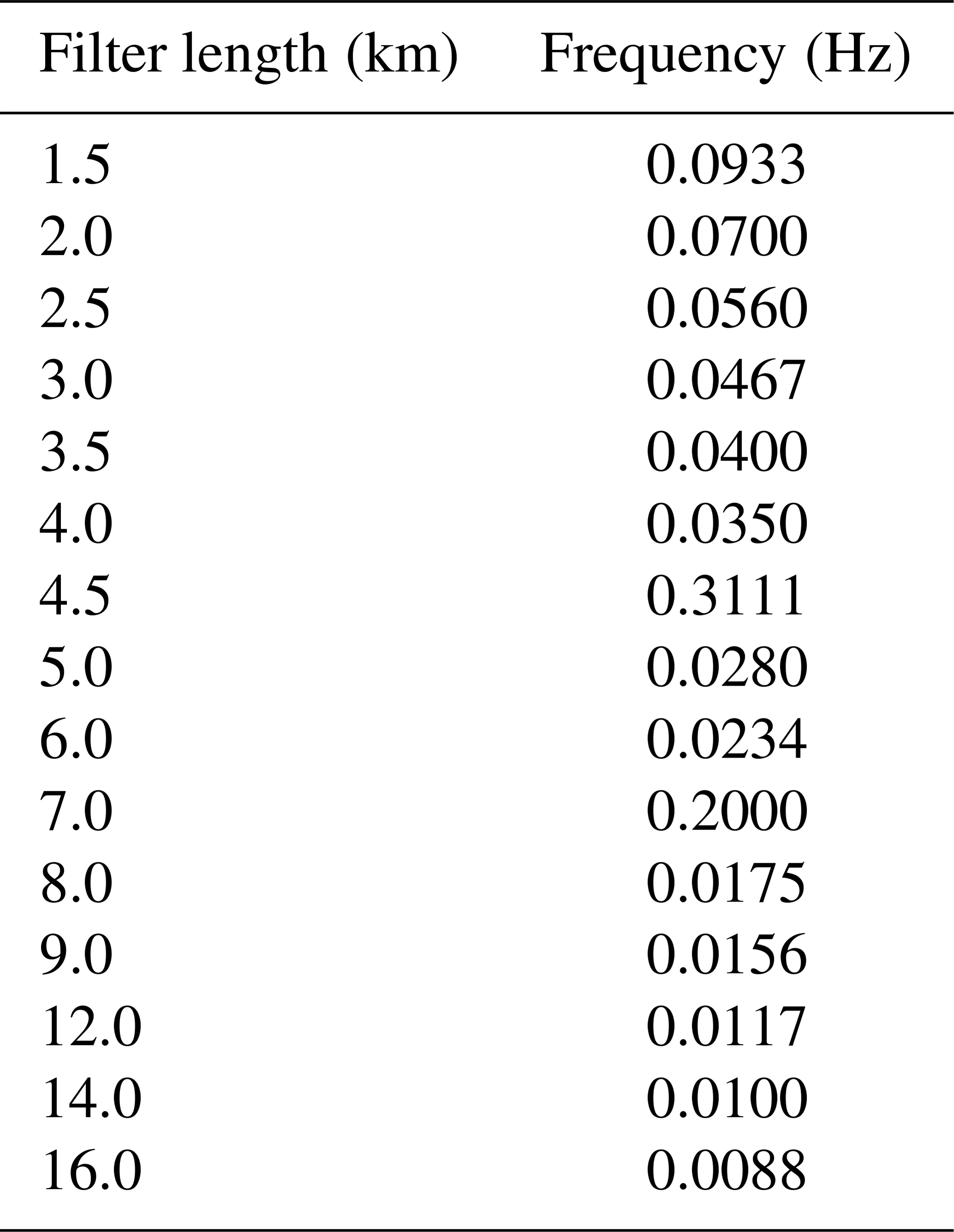
To enable use of wind data from slant profiles, the three-dimensional wind components were filtered using a four-pole Butterworth high-pass filter, following the studies of Lenschow et al. (1988) and others (e.g. Mahrt, 1985; Brooks et al., 2003), who have used this method for analysis of stable boundary layers. All data from both slant profiles and geometrically level flight segments were included outside of turns. Investigation of the length scales of turbulence in the system were investigated by applying a range of Butterworth filters (see Appendix B) with filter lengths between 1.5 and 16 km (Table B1). Turbulence kinetic energy (TKE) was computed from the residual high-frequency fluctuations in three dimensions, for each length of filter, using

Application of Taylor's frozen-turbulence hypothesis (Stull, 1997) permits the compositing of data from throughout the measurement period on to a “virtual meteorological mast” floating in the free troposphere.

Figure 3 shows the flight profile on a latitude–altitude cross section. The potential temperature (θ) measurements, although not uniformly distributed throughout the section, were interpolated in latitude–altitude space to give an overview of the thermodynamic environment in which the cloud was found. The liquid water content from the CDP and ice number concentration (N_I) from the CIP15 are plotted and show the spatial cellular structure of the liquid water and vertical structure of the cloud system.

Figure 3Aircraft altitude as a function of latitude from flight B674 (2 February 2012; black line), LWC from CDP (blue circles) and N_I from CIP15 (red triangles). Potential temperature (θ) observations are interpolated in latitude–altitude space (greyscale contours).

Download

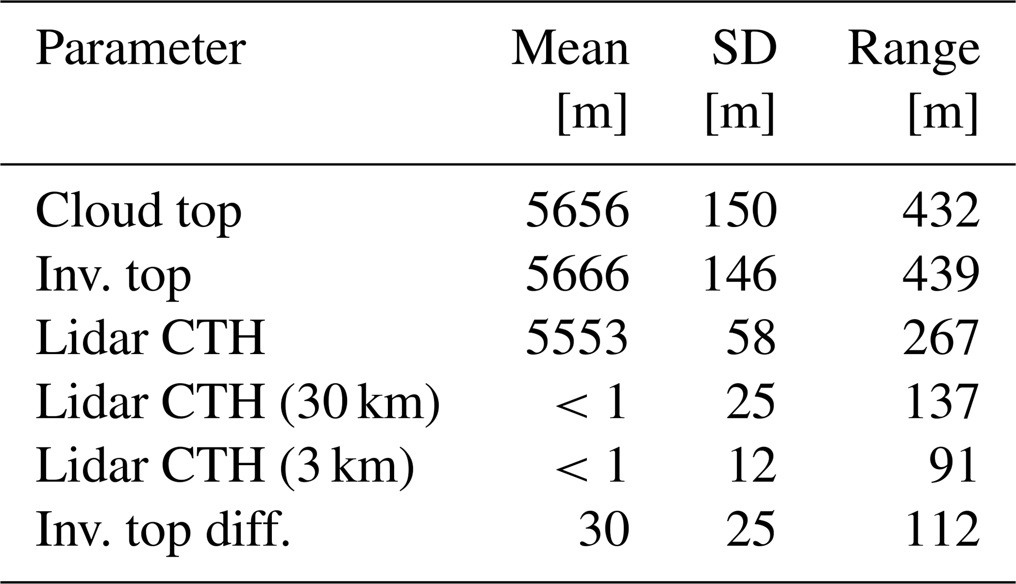
The CTH derived from profile observations as a function of time and latitude was extrapolated back in time to allow comparison with the lidar-derived CTH observations from the earlier above-cloud run. Residual differences between the derived time series of CTH and lidar CTH were typically less than 50 m and in all cases less than ≈100 m (see Table 2). De-trending the lidar CTH data at two scales, 30 and 3 km, shows that the range of CTH was of a similar order to the uncertainty. The standard deviation of CTH at the 30 km scale was of the order of 25 m and at a 3 km scale was close to 12 m, with the two scales perhaps corresponding to the altocumulus cell scale (3 km) and gravity wave structures (30 km).

Table 2Cloud top height derived from CDP LWC, inversion altitude derived from temperature profiles, lidar-derived CTH (and with 30 and 3 km trends removed), and difference (residual) between the measured inversion altitude and the derived inversion altitude, shown in terms of mean, standard deviation and range.

Download Print Version | Download XLSX

With distance from inversion altitude as the vertical coordinate it can be seen that there was an inversion in potential temperature of the order of 3 ^∘C that extended over less than 100 m (Fig. 4). Below the inversion was a seemingly well-mixed layer in terms of potential temperature, for at least 600 m below the inversion. The air was much drier above the inversion where relative humidity w.r.t. liquid fell from saturation at the top of the layer to ≈50 % above the inversion (Fig. 4c). Ice supersaturation extended down through the top 500 m of the cloud layer. The liquid cloud at the top of the layer had a depth of just over 200 m with a maximum coverage of 0.8 just below the inversion (Fig. 4d). Ice cloud fraction was close to zero at the top of the liquid cloud layer, increasing with depth below this to a similar value close to 0.8 some 300 m below cloud top.

Figure 4Vertical profiles of statistics w.r.t. inversion altitude, Δz_(inv.), for (a) dew point (black), as well as mean and standard deviation of temperature (red), and (b) potential temperature and (c) relative humidity w.r.t. ice (blue) and liquid (black). The boxes indicate the interquartile range (two-dimensional), the whiskers indicate the 5th and 95th percentiles, and the filled triangles indicate the 1st and 99th percentiles. (d) Areal cloud fraction calculated from number concentration of liquid (CDP) (solid black) and ice particles (CIP15) (solid blue) over 40 m altitude bins, with dashed lines showing the volume mean equivalent fraction over a 600 m deep layer (black is liquid and blue is ice) and calculated mixed-phase cloud fraction in this layer assuming maximum overlap (dotted–dashed black line).

Download

The current generation of operational NWP models have a typical vertical resolution of the order of 600 m in the mid-troposphere (Walters et al., 2017). If the cloud fraction (cf) observations were to be volume-averaged over the full depth of the cloud layer, cf^grid (similar to a typical NWP grid box depth), then the volume cloud fractions of the liquid and ice parts of the cloud are cf${}_{\mathrm{liquid}}^{\mathrm{grid}}\le \mathrm{0.25}$ and cf${}_{\mathrm{ice}}^{\mathrm{grid}}\le \mathrm{0.60}$. The resulting mixed-phase cloud fraction is therefore cf${}_{\mathrm{mixed}}^{\mathrm{grid}}\le \mathrm{0.15}$. The maximum value assumes that both liquid and ice are evenly distributed throughout the volume, something the observations do not support: liquid is concentrated in the top third of the cloud layer, and ice is concentrated in the lower two-thirds. This greatly reduces the volume in which liquid and ice are expected to co-exist, which has important consequences for mixed-phase microphysical processes in NWP simulations. Microphysical aspects of the cloud are discussed in detail in Sect. 4.2.

In the following section the analysis begins to focus on the vertical structure of the observed vertical velocity fluctuations in the cloud layer system described above.

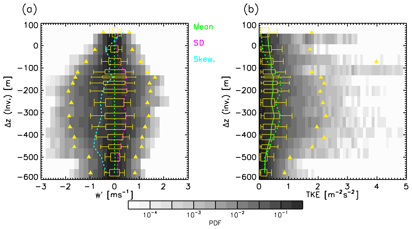
Figure 5Two-dimensional histograms for 9 km filtered data against distance from inversion altitude for (a) vertical velocity fluctuations, w^′ and (b) TKE, with a PDF (probability distribution function) of 32 Hz data (greyscale) and percentiles (yellow) also shown. (a) Mean value of w^′ (green), standard deviation of w^′ (magenta) and skewness of w^′ (cyan). (b) Mean value of TKE from the three component winds (solid green) and only the vertical component (see text for details) (dashed green).

Download

4.1 Vertical profiles of TKE and vertical velocity distribution

Figure 5 shows profiles of vertical wind fluctuations, w^′ (Fig. 5a) and TKE (Fig. 5b) constructed from raw data with a high-pass Butterworth filter that is 9 km in length (see Appendix B). The percentiles are shown in 20 vertical levels, with each representing 25 km of measurements. Vertical velocity fluctuations (Fig. 5a) ranged between −3 and +2 m s⁻¹, and the variability, characterised by the standard deviation of w^′, increased from the inversion top to a maximum of 0.5 m s⁻¹ at −150 m and remained reasonably constant to −400 m before diminishing by −600 m. The skewness of the distribution of vertical velocity fluctuations is increasingly negative with distance below cloud top, as the spectra of w^′ becomes increasingly dominated by downdraughts. The TKE profile (Fig. 5b) shows median values close to 0.5 m² s⁻² in a layer from −150 to −400 m, below which they reduce. Horizontal high-pass filtered wind components, u^′ and v^′, have higher-magnitude residual mean values close to the inversion compared to w^′, a result of slight wind shear across the inversion and contamination by the filter. This will result in spuriously large values for TKE in this region. By substituting the vertical velocity fluctuations, w^′, in place of u^′ and v^′ in the calculation of TKE (Eq. 1) it can be seen that the turbulence kinetic energy tends towards zero and increases steadily below cloud top towards the local maxima at −150 m. Below this altitude the estimate of TKE using only w^′ is biased high as compared to the full three-dimensional estimate.

Vertical velocity fluctuation probability distribution functions (PDFs) as a function of distance from inversion altitude are presented in Fig. 6 for five vertical ranges. The highest level, within cloud tops, centred on $\mathrm{\Delta }{z}_{(\mathrm{inv}.)}=-\mathrm{50}$ m, had a narrow w^′ distribution with low skewness (−0.23), and had a range that was predominantly ±1.0 m s⁻¹. Within the bulk of the liquid cloud, centred on −150 m, the range was larger with peak updraughts of 1.5 m s⁻¹ offset by stronger maximum downdraughts of −2.0 m s⁻¹, resulting in low skewness of −0.20. Peak updraughts were weaker in the next vertical level down, centred on −250 m and roughly corresponding to the cloud base layer and start of sub-cloud virga, where negative skewness developed to −0.62. Deep within the virga layer at −400 m there will still be moderate updraughts generated, but the magnitude of the skewness was largest at −0.79, relaxing to −0.44 at −550 m. The PDF at the lowest level showed that most fluctuations were of low magnitude, similar to cloud top, but occasional strong downdraughts up to −1.5 m s⁻¹ were present and still influenced by LWRC from cloud top.

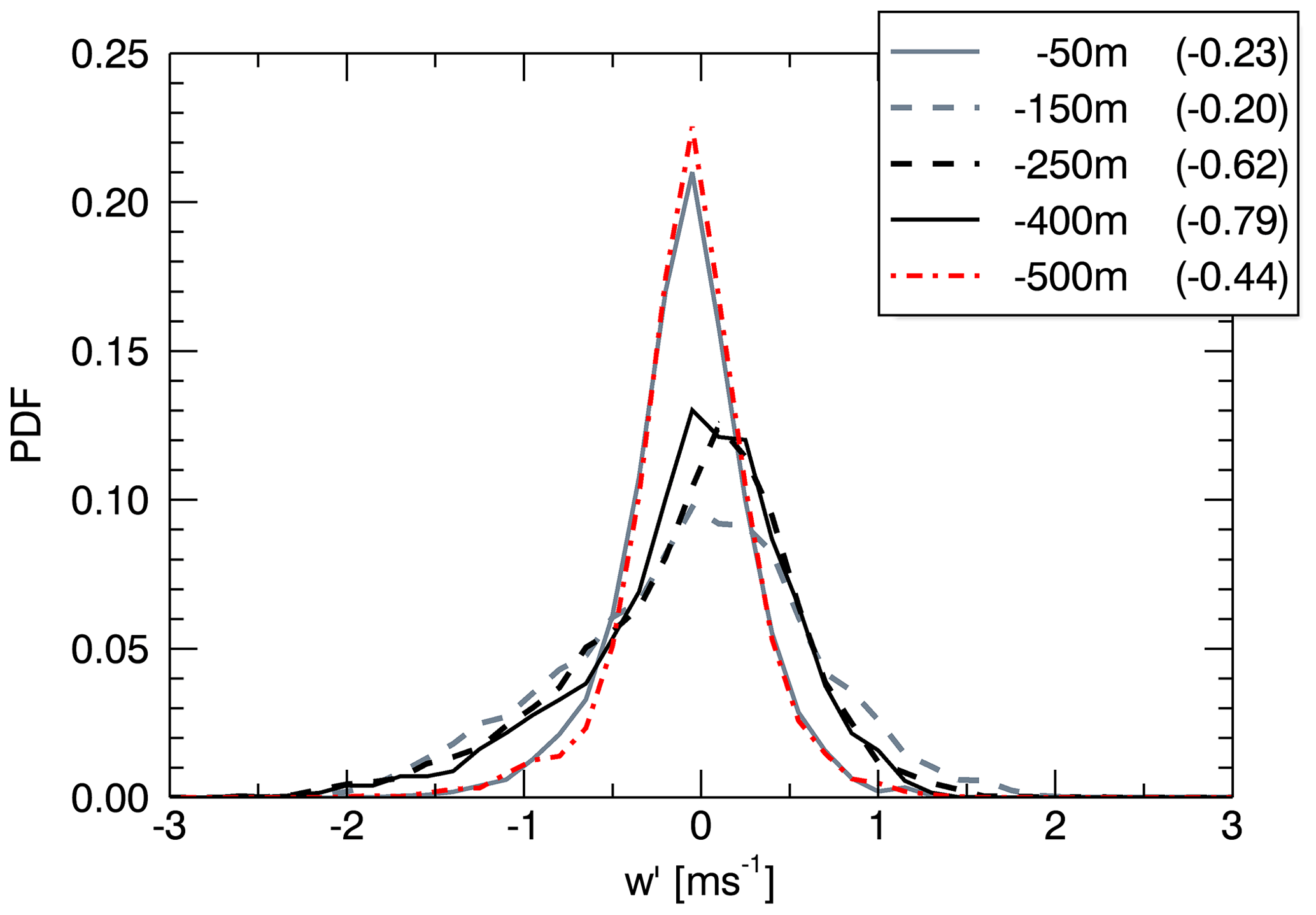
Figure 6Vertical velocity fluctuations PDFs from five altitudes below inversion altitude with levels given in the legend. The first value gives the centre altitude of the level, with the second number giving skewness of the vertical velocity distribution. Standard deviations of depth in each level were between 15 and 50 m.

Download

The impact of filter length on the measurements is explored to provide information about the length scales that are operating within the cloud system (Fig. 7). Close to cloud top at −50 m, both TKE (standard deviation) and skewness are low and vary little as a function of length scale. Within the liquid cloud layer at −150 m, the TKE is observed to peak and is dominated by longer length scale circulations. There is low-magnitude negative skewness to the distribution of vertical velocity fluctuation, consistent for all filter lengths: here the induced updraughts are almost sufficient to offset the negative skewness introduced by the downdraughts. Just below the liquid cloud is where a separation of skewness as a function of length scale becomes apparent, whilst TKE is generally similar to the level above. By 250 m below cloud top the magnitude of the skewness has doubled in general, with a slightly stronger increase for longer filter lengths. Below −400 m the downdraughts begin to dominate the spectra, with the magnitude of skewness with a 9 km being 50 % larger than for a 1.5 km filter, although the overall magnitude of turbulence intensity tends to reduce. The lower-magnitude skewness for shorter length scales at this altitude implies that resultant updraughts occur at smaller scales than the downdraughts driving the circulation. Updraughts are occurring on a scale of the order of a few hundred metres, compared to a couple of kilometres for downdraughts. The strongest difference between long and short filter lengths is apparent at −500 m, although the overall magnitudes of skewness are lower, implying that the few downdraughts that penetrate this low do not have as large an impact in driving updraughts, possibly due to reduced convergence between ever less frequent cold pools to this depth. Turbulence intensity is a factor of 4 lower than the peak.

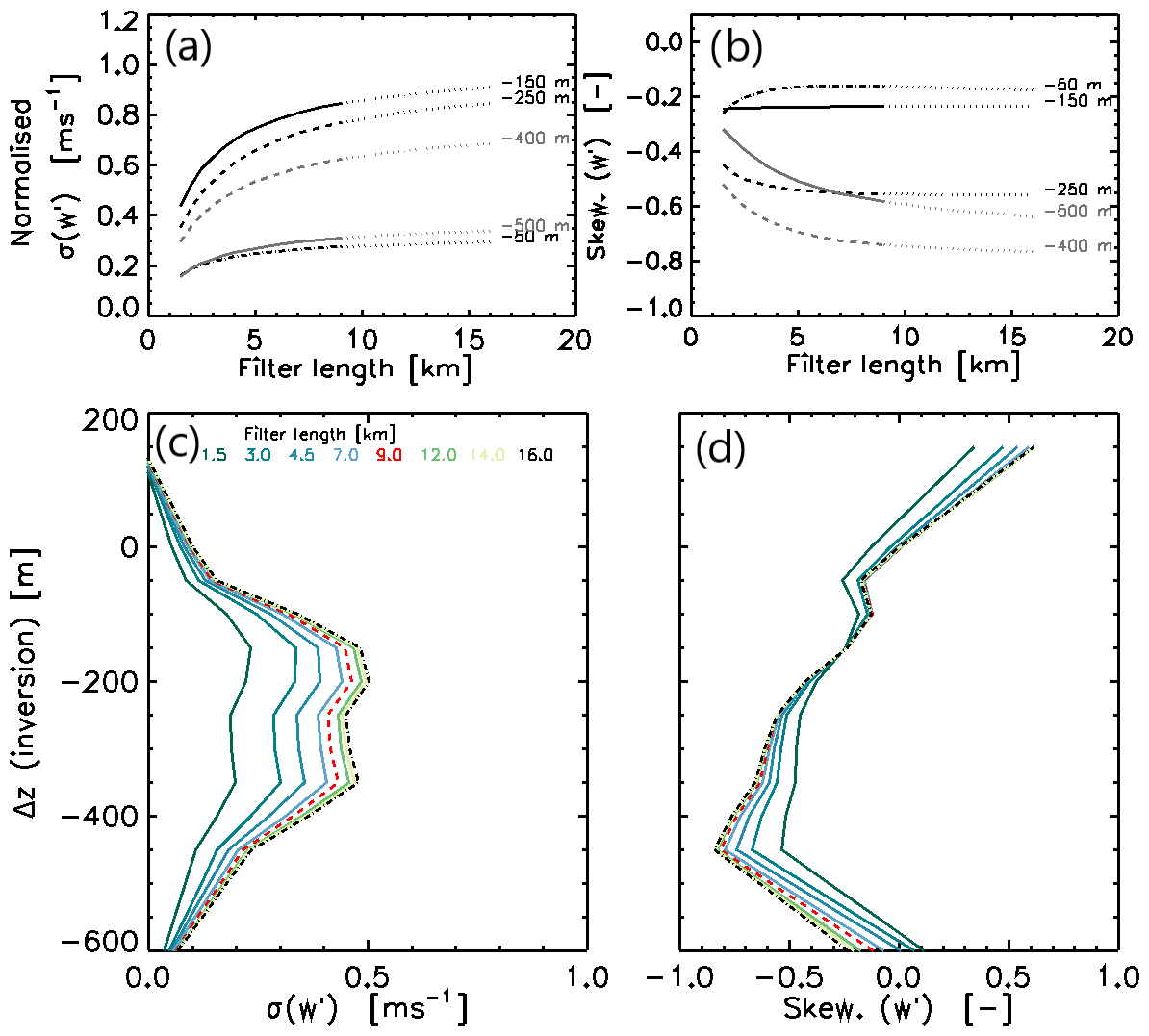
Figure 7(a) Standard deviation of w^′ as a function of filter length, normalised to the layer maximum value for five altitudes below the inversion altitude. Length scales longer than the chosen 9 km filter length are shown with dotted line to indicate how much of the variance is at scale that pass through this filter. (b) Skewness of distribution of w^′ as a function of filter length, normalised to layer absolute maximum value, the same as in (a). (c) Vertical profile of standard deviation of w^′ relative to the inversion altitude for a range of filter lengths from 1.5 km (blue) to 14 km (green) and the limit of 16 km (dotted–dashed black); 9 km is highlighted with dotted red. (d) Vertical profile of skewness of the distribution of w^′ relative to inversion altitude, as (c).

Download

4.2 Cloud and aerosol microphysical observations

The updraughts are responsible for the maintenance of the supercooled liquid cloud layer. The liquid water content profile as measured by the Nevzorov LWC sensor is shown in Fig. 8 with data plotted with respect to Δz_(CTH). The data show a sub-adiabatic profile of liquid water content for the majority of observations but with the extreme largest values being close to adiabatic.

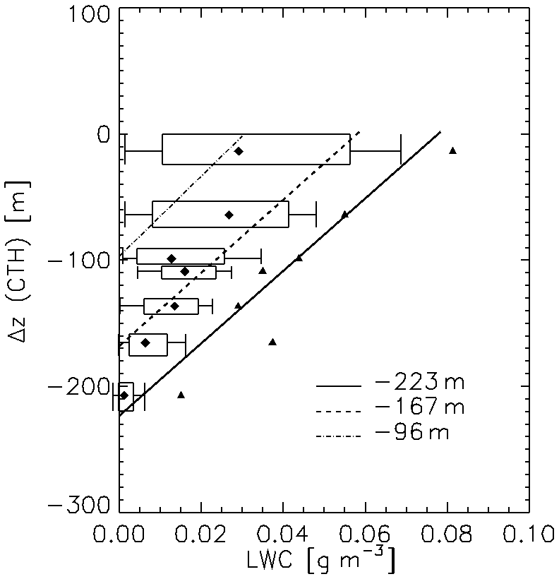
Figure 8LWC profile percentiles relative to CTH for the mixed-phase cloud layer with data from Nevzorov LWC sensor. Theoretical adiabatic ascents are shown, starting from three altitudes (see legend for details), which correspond to potential cloud bases (see text for details). Statistics are the same as in Fig. 4.

Download

Theoretical, undiluted adiabatic LWC profiles were calculated by assuming an ascent of a saturated air parcel from three initial altitudes corresponding to potential cloud bases. The first, from the minimum liquid cloud base at −223 m, shows that peak observed cloud top LWC values compare well with this theoretical estimate. An ascent from −167 m peaks close to the 75th percentile of cloud top LWC. A third ascent from −97 m has a peak LWC close to the 50th percentile at cloud top. Whilst entrainment of dry air from aloft at the inversion may be non-zero, these calculations demonstrate that the non-uniform cloud base may have contributed to the observed in-cloud variability in LWC at a given level. This suggests a range of turbulent eddies and updraught depths contributed to the overall spectrum of in-cloud liquid water contents.

Now the full mixed-phase cloud system is considered. Statistics were calculated for vertically resolved liquid and ice particle in-cloud number concentrations (Fig. 9a), effective radius (Fig. 9b), and condensed water content (Fig. 9c). Vertical layers of ice supersaturation frequency are shown to aid interpretation.

Figure 9Vertical profiles relative to cloud top of (a) cloud particle number concentrations of liquid, N_d, (CDP, cm⁻³; blue) and ice, N_i, (CIP15, L⁻¹; orange) and (CIP100, L⁻¹; light brown), (b) effective radius for liquid cloud particles, R_eff(liquid), (CDP; blue) and ice particles R_eff(ice), (CIP100; light brown). (c) Condensed water content (CWC) with LWC (CDP; blue) and IWC (CIP15; orange). The altitude of observed frequency (areal fraction) of ice supersaturation is shown for 100 % (dashed black line), 50 % (dashed–dotted black line) and 25 % (dotted black line).

Download

Cloud drop numbers were constant in-cloud at ≈30 cm⁻³, implying nucleation at cloud base (Fig. 9a). Cloud top liquid particle effective radius was typically observed in the range 11 to 15 µm (interquartile range), with smaller particles close to cloud base (Fig. 9b). As previously shown (Fig. 8), the largest LWC values were at cloud top, peaking close to 0.1 g m⁻³. Liquid cloud particle size distributions were as expected, with cloud particles growing in size towards cloud tops (Fig. 10). These composite distributions, segregated by distance from cloud top (Table 3) show that clouds bases typically have high number concentrations of small particles below the mode of ≈11 µm and very few particles larger than 20 µm. Within the mid-cloud layer there are greater concentrations of larger particles and a similar mode. At cloud tops the largest particles are about 30 µm and concentrations of particles smaller than 10 µm are reduced compared to the layers below, whilst the mode remains constant.

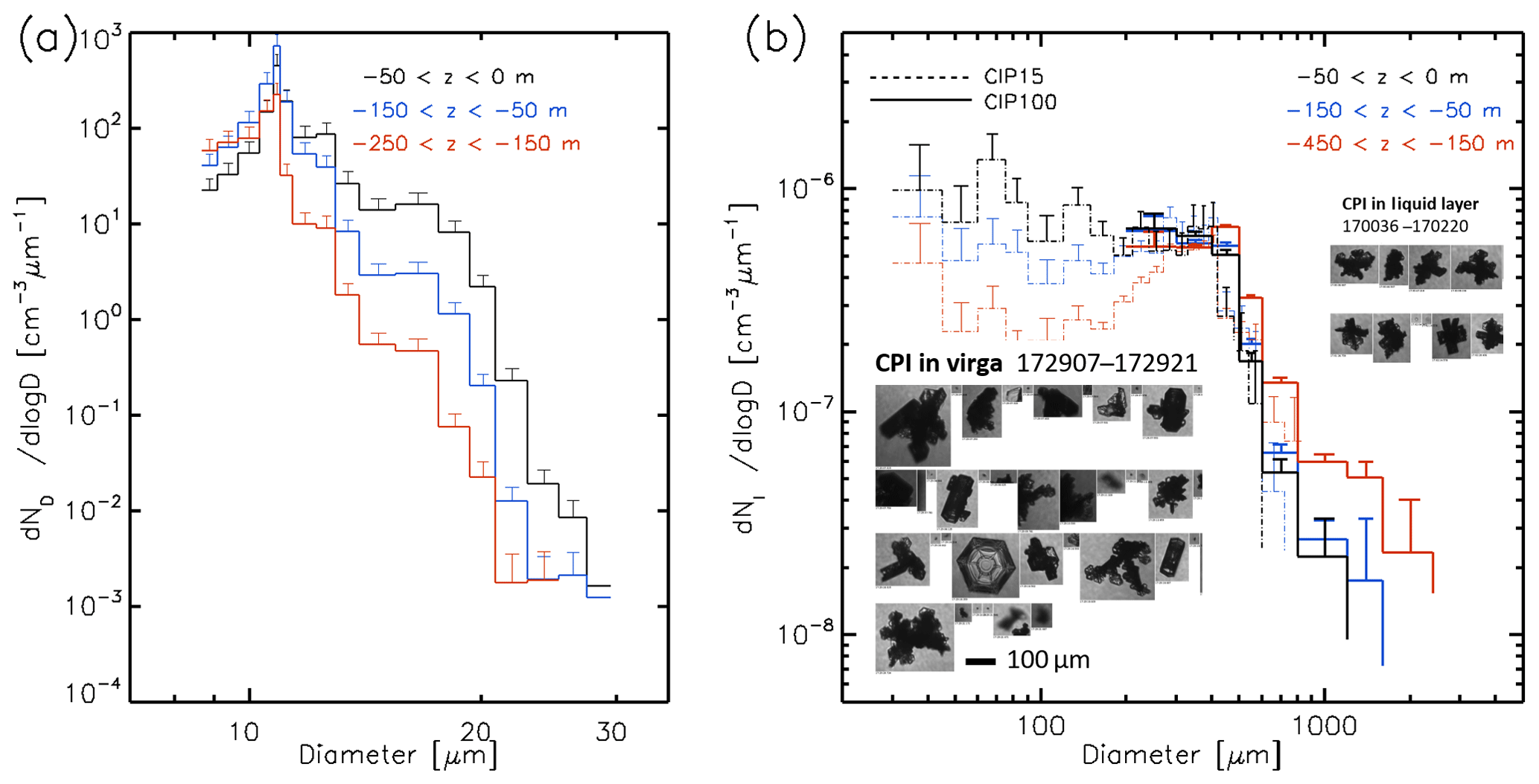
Figure 10(a) Mean liquid cloud particle size distributions for three vertical levels as Table 3, with cloud top level (black), mid-cloud (blue) and cloud bases (red). Error bars represent standard deviations. (b) Ice particle size distribution from CIP15 (dashed line) and CIP100 (solid line) with colours the same as in (a) and vertical levels the same as Table 3. Example particle images are taken from CPI probe in ice virga and from within the mixed-phase cloud regions, and the scale bar is shown for 100 µm length, along with the time range of the imagery.

Download

Table 3Vertical level (w.r.t. CTH) ranges for liquid particle size distribution (PSD) from CDP and ice PSD from CIP probes and layer temperature ranges, with the distance spent sampling at that level along with time spent sampling mixed-phase (MP) clouds, number of cloud drops larger than given diameter and size-resolved ice production rates. ^* Lower level is deeper for CIP data.

Download Print Version | Download XLSX

Median ice particle number concentrations measured by CIP15 were of the order of 0.5 to 5 L⁻¹, peaking just below the liquid cloud base and remaining approximately constant below this whilst reducing with altitude towards the top of the liquid cloud (Fig. 9a). Data from CIP100 showed a similar trend, with a peak concentration just below cloud base and the concentrations falling off more rapidly towards cloud top than data from the CIP15, where particles tend to be smaller. Ice particle effective radius (Fig. 9b; shown for CIP100, which has a larger sample volume) increased with depth from liquid cloud top to a maximum value close to 300 m below cloud top. Peak IWC was slightly greater than peak LWC (Fig. 9c), whilst median values were lower in magnitude. Ice particles were not found at the very top of the liquid layer and their concentration peaked in magnitude below the liquid cloud bases. Ice supersaturation frequency (Fig. 9) fell below 100 % at a level of 350 m below cloud top. IWC reduced below 600 m, where ice supersaturation frequency fell below 25 %. Effective diameter decreased below 500 m, where the ice supersaturation frequency was less than 50 %. Ice properties remained consistent, even when ice supersaturation frequency reduced, suggesting that the ice particles initially fell within branches of descending air with larger values of ice supersaturation.

Observations of ice number, effective radius and IWC are consistent with ice nucleation occurring within the liquid cloud. Following this, ice particles continue to grow and sediment through the ice supersaturated layers beneath. Mean ice particle size distributions are plotted in Fig. 10b according to the vertical levels in Table 3 to show the properties of the ice virga. Number concentrations of the smallest particles are much larger for the very top level in cloud, perhaps identifying the ice particle generation zone. Below this cloud top layer, the cumulative particle volume distribution has a constant slope up to a size of 300 µm, implying that the same process is responsible for the ice production, i.e. diffusional growth. Particle imagery from CPI (Fig. 10b) showed the dominant ice particle type to be complex polycrystalline structures (also observed by Korolev et al., 2000), which likely grew as single crystals, followed by aggregation to larger sizes. The particles share many features of “assemblages of large plates” that are present at temperatures close to −30 ^∘C above water saturation (see Fig. 5 in Bailey and Hallett, 2009). Some evidence of riming was present within the liquid layer.

The ice production rate for these altocumulus clouds was calculated in a manner similar to Harris-Hobbs and Cooper (1987), with the addition that the rate was computed between adjacent pairs of size channels (which have a width of 15 µm) for CIP15 data up to 400 µm (full details in Appendix C). Data were selected from mixed-phase regions (N_d>5 cm⁻³ and N_i>0.1 L⁻¹ for particles with diameters larger than 100 µm) for the initial cloud sampling period between 17:00 and 17:30 UTC and in the three vertical levels defined in Table 3. The results are shown in Fig. 11. Peak rates are notably greater for the level nearest to the cloud top and for sizes smaller than 140 µm. At this cloud top level there are very little data for sizes larger than 230 µm. For the two lower levels within the liquid cloud there is general similarity between the computed ice production rates. A summary of these results can be found in Table 3, which presents weighted mean ice production rates for groupings of adjacent size channels on CIP15, in the size ranges 60–105, 120–225 and 240–345 µm. For the smallest particles (D<105 µm), the rate of ice production near cloud top is double that at the level below and a factor of 3 larger than at cloud base, which supports the suggestion that ice nucleation occurs at cloud top.

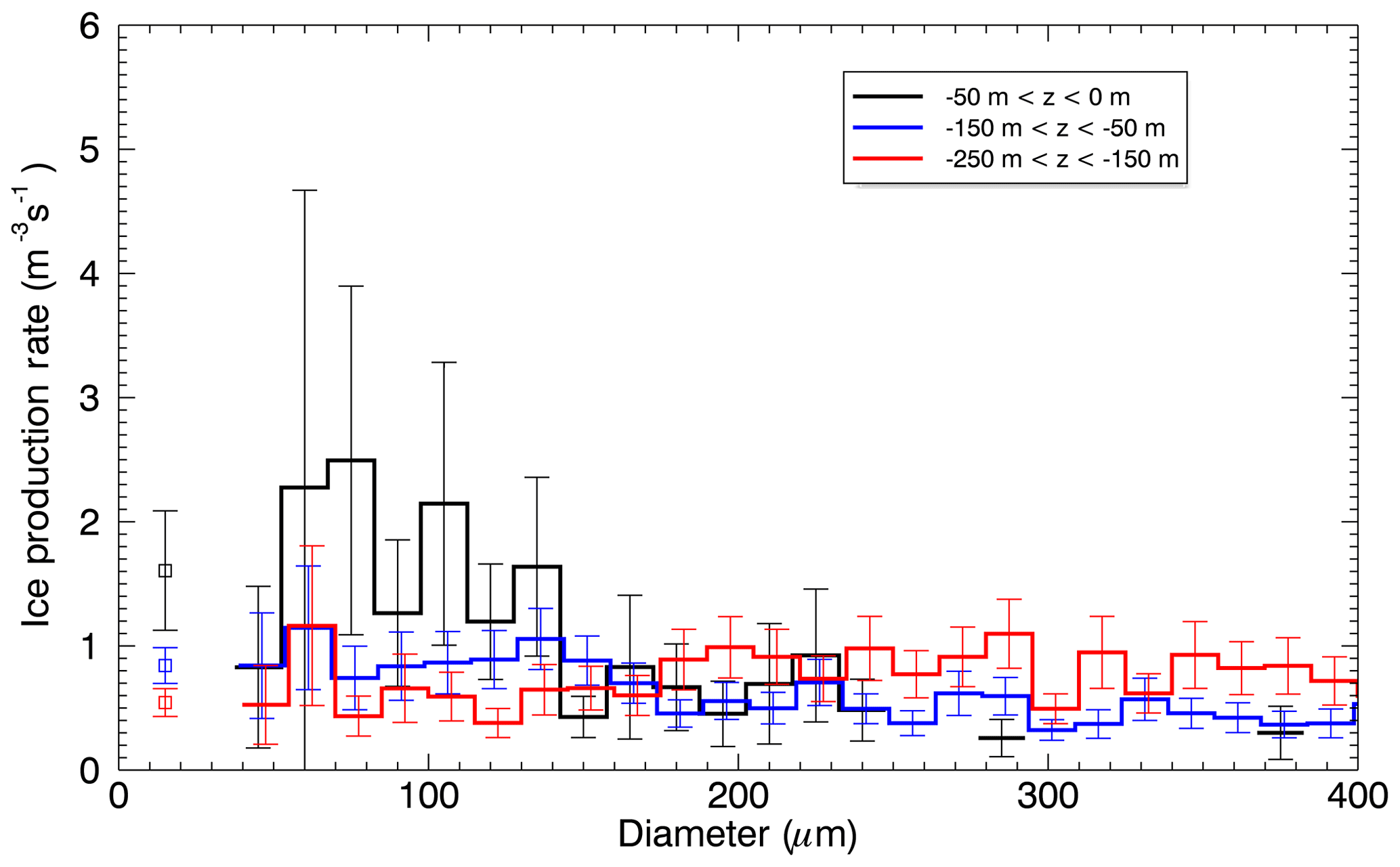
Figure 11Ice production rate for three levels (Table 3) in altocumulus cloud with −50 m < z < 0 m (black), −150 m < z < −50 m (blue) and −250 m < z < −150 m (red), computed between adjacent channels of CIP15 data between 45 and 400 µm. Weighted mean values and errors are shown for the smallest particle size range (as Table 3) at all three levels with squares and errors bars.

Download

As mentioned in Sect. 3, ice-nucleating particles were not observed directly. Total aerosol number concentration (accumulation mode) and concentrations of the larger particles are shown in Fig. 12a for two layers, one above cloud and one within the cloud layer, when out of cloud and precipitation. The observed number concentrations of aerosol particles larger than 0.5 µm from PCASP (Fig. 12a) were used as inputs into the parameterisations of DeMott et al. (2015) for general aerosol and Tobo et al. (2013) for forest sources of aerosol (Fig. 12b). Back trajectories (not shown) indicate a source region for the air mass over the boreal forests of North America with large-scale ascent in the mid-latitude storm tracks providing a potential uplift mechanism. A nucleation temperature of −30 ^∘C was applied, assuming nucleation occurred at cloud top. Number concentrations of aerosol particles larger than 0.5 µm are of the order of 0.07 cm⁻³, both above and within the cloud layer. Resulting INP concentrations are N_INP=1.0 L⁻¹ (DeMott et al., 2015) and 0.60 L⁻¹ (Tobo et al., 2013). Observed ice number concentrations are plotted in Fig. 12c from CIP15 and CIP100. Observed ice concentrations compare closely with the INC-corrected INP concentrations, particularly for the CIP15, which is able to observe smaller ice particles, and for the forest emissions parameterisation of Tobo et al. (2013). Whilst the observations show that there are larger concentrations of accumulation mode aerosols within the cloud layer than above it, the same cannot be said for number concentrations of aerosols larger than 0.5 µm, limiting the ability of the data in this study to distinguish the source of the INP particles. Peak accumulation mode aerosol particle number concentrations are below 10 cm⁻³, thus some particles smaller than 0.1 µm must have acted as CCN (cloud condensation nuclei) to produce a cloud with droplet concentrations of 30 cm⁻³.

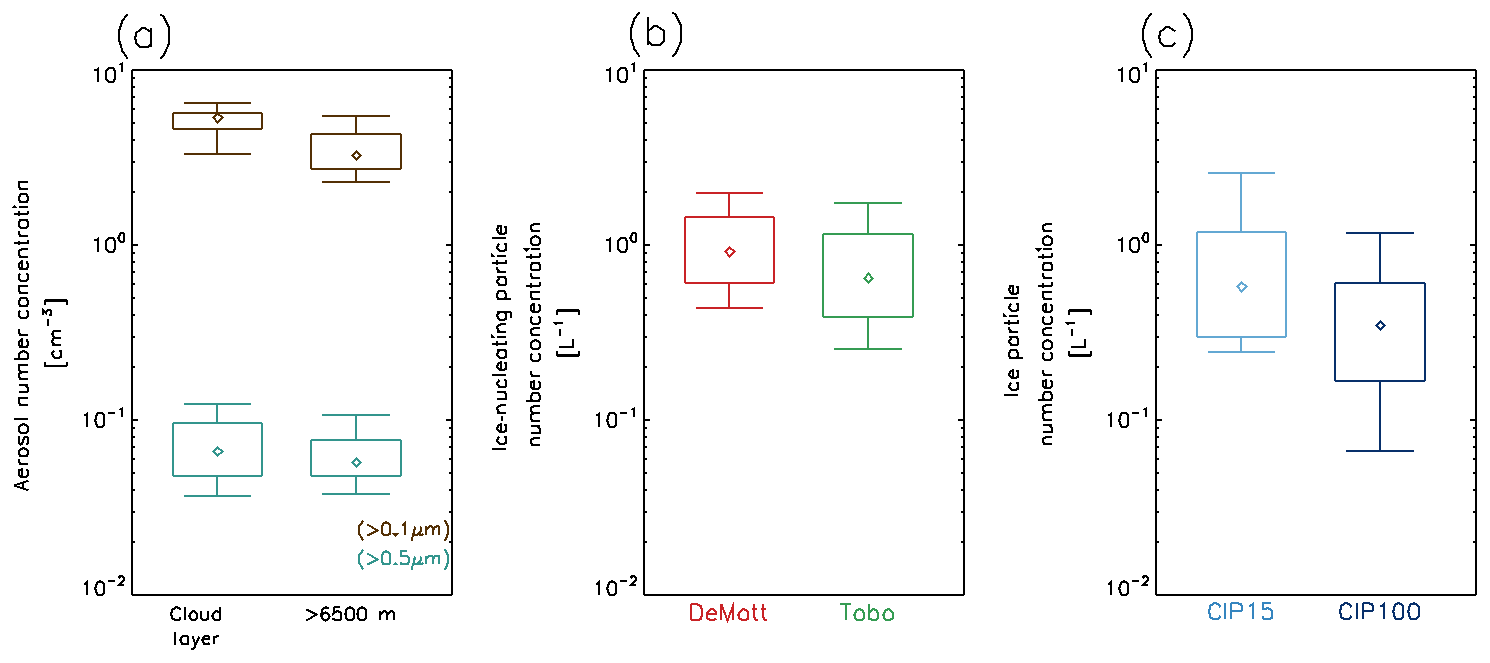
Figure 12(a) Percentiles of aerosol particle number concentrations larger than 0.1 µm (brown) and 0.5 µm (teal) from PCASP for the cloud layer (left) and above 6500 m (right). (b) INP concentrations (L⁻¹) using DeMott et al. (2015) (red) and Tobo et al. (2013) (green). (c) Ice particle number concentrations N_i from CIP15 (light blue) and CIP100 (dark blue).

Download

The measurements presented show a highly supercooled altocumulus layer cloud, with precipitating ice virga. Along with previously published results from the literature, the life cycle of altocumulus clouds will now be considered. Supersaturation and hence liquid cloud formation in the mid-levels of the troposphere may be achieved through large-scale ascent with upwards air motion accentuated through wind shear or gravity wave activity or convective detrainment at a stable interface (Rauber and Tokay, 1991) (Fig. 13a), where the distribution of relative humidity with respect to liquid permits. Ansmann et al. (2009) showed that for tropical altocumulus clouds the liquid phase is always present before the ice phase, and Westbrook and Illingworth (2011) found that for mid-latitude clouds observed from the ground that liquid cloud layers are situated above ice clouds in the majority of cases warmer than −27 ^∘C.

Figure 13Schematic of processes that control altocumulus clouds as a function of normalised cloud layer depth below cloud top altitude, Z. The lower boundary is typically diffuse, unlike for stratocumulus, which has the surface as a lower boundary (a) cloud formation through large-scale ascent, possibly augmented by wind shear or gravity wave activity acting at a stable interface in potential temperature (θ: black trace), with a suitable relative humidity distribution (solid blue: RH w.r.t. liquid; dashed blue: RH w.r.t. ice; arrows indicate distribution up to 100 %) just below the temperature inversion. (b) Clouds (blue parcels) cool through long-wave radiative cooling from cloud top, a process which imparts turbulence to the layer below with narrow strong downdraughts (blue arrows) and broad weaker updraughts (red arrows). (b-i) to (b-v) See text for details of the resulting turbulence structure. (c) Turbulence acts to maintain the liquid water content profile (blue line) in a pseudo-adiabatic form (dashed black line). (d) At temperatures lower than 0 ^∘C, ice nucleation may occur, located within the liquid cloud, resulting in ice precipitating from the liquid cloud layer. (e) The turbulence kinetic energy peak occurs below the liquid cloud layer, with the skewness of the vertical velocity distribution occurring lower still.

Download

Once the formation of liquid has occurred, cooling from cloud top through emission of long-wave radiation to space will generate negatively buoyant air parcels that will tend to descend through the cloud layer. Descending air parcels occur in narrow downdraughts and through mass continuity force upward motion that, dependent on humidity, may continue to support the production of supersaturation and hence liquid water. A more detailed discussion is presented below. Figure 8 shows that the observed liquid water content followed a pseudo-adiabatic profile; see Fig. 13c.

At some later stage, where the liquid clouds reside at temperatures colder than 0 ^∘C, the production of ice may occur (Fig. 13d). The computation of ice production rate suggests a tendency towards ice production close to cloud top (Fig. 11), as depicted in Fig. 13d-i, but the increase in both ice number concentration and ice mass with distance below cloud top (Fig. 9a and c) indicates that the production of ice occurs at all levels within the liquid cloud. Number concentrations of ice particles remain constant in the ice-supersaturated layer below the liquid cloud (Fig. 9a), indicating that ice nucleation is not active in that region (Fig. 13 d-ii). The negatively skewed vertical velocity distribution (Fig. 6) is similar to that found in nocturnal stratocumulus (Nicholls, 1989). Hogan et al. (2009) (Fig. 13b) found a similar profile of skewness for LWRC-driven nocturnal stratocumulus clouds using ground-based measurements, in contrast with the profiles of skewness that were obtained when surface-heating-driven cumulus clouds were overhead. The turbulence kinetic energy spectra are also similar to those found in stratocumulus (Ghate et al., 2014) (Fig. 13e). The eventual dissipation of the altocumulus clouds may occur through erosion of humidity within the cloud layer through precipitation or an increase in subsidence, which would act to warm the layer (Larson et al., 2006). Likewise, turbulent mixing and radiation can also be important.

The turbulence observations presented in Sect. 4.1 will now be placed into context by comparing them with the remote-sensing observations and derived conceptual model of Schmidt et al. (2014) of the circulation structures within altocumulus clouds. Other observations from ground-based studies conducted in both the tropics and mid-latitudes, as well as previously published in situ observations, will be drawn upon where appropriate. At the top of the cloud, where $\mathrm{\Delta }{z}_{(\mathrm{inv}.)}=-\mathrm{50}$ m (Fig. 6), these in situ observations show a narrow distribution of w^′ with a low skewness value, features which are likely to be characteristic of shallow cloud top eddies, similar to those resolved by the remote-sensing observations in Fig. 7 of Schmidt et al. (2014): at this level, close to the inversion, the broader and deeper circulations do not have the opportunity to develop, as depicted in Fig. 13b-i.

The PDF of w^′ at $\mathrm{\Delta }{z}_{(\mathrm{inv}.)}=-\mathrm{150}$ m has positive and negative fluctuations of almost equal magnitude and hence low skewness (Fig. 6), which therefore corresponds to the Schmidt et al. (2014) “cloud layer” where Rayleigh–Bénard type cells were observed (Fig. 13b-ii). Schmidt et al. (2014) also found a symmetrical distribution of vertical velocities on a horizontal scale comparable to or just larger than the liquid cloud depth. The previous in situ observations of turbulence in altocumulus clouds (Watson, 1967; Fleishauer et al., 2002) were made within the liquid layer and therefore all correspond to these liquid layer observations and show similar magnitudes. Ansmann et al. (2009) and Simmel et al. (2015) both presented remote-sensing results for the liquid portion of altocumulus clouds with similar magnitudes and distributions.

Altocumulus clouds often occur in multiple layers (Korolev and Field, 2008; Fleishauer et al., 2002). These could form when the resulting updraughts produce liquid supersaturation at a level below the cloud layer driving the turbulence (Fig. 13b-iii). It is possible that long-lived altocumulus clouds such as those observed by Westbrook and Illingworth (2013) and Carey et al. (2008) were maintained through a particular set of conditions, including vertical stability and the distribution of humidity, which permitted the formation of secondary “daughter cells” at the same altitude as the driving clouds.

Within the ice virga, between −250 and −400 m below cloud top (Fig. 6), the observed turbulence properties differed from those found in the liquid cloud layer with a shift to increasingly negative skewness; these results are consistent with the “Subcloud Layer 1” of Schmidt et al. (2014), corresponding to Fig. 13b-iv, with downwards penetrating mammatus type features. This connection between the liquid cloud layer and below was observed by Schmidt et al. (2014) to be on a longer length scale than the in-cloud circulations of the order of 1 km. Ansmann et al. (2009) presented turbulence observation from within the ice virga layer (using radar sensitive to the larger ice particles) for late-stage development clouds, which showed a shift to negative skewness, −1.75 m s${}^{-\mathrm{1}}<w^{\prime }<\mathrm{0.75}$ m s⁻¹, and an increase in standard deviation of w^′, comparable to the direct turbulence observations presented here. Unlike remote-sensing-derived observations of turbulence, these in situ measurements are not reliant on, or biased by, observations of, or assumptions about the ice particle size distribution. At the lowest level of the in situ observations ($\mathrm{\Delta }{z}_{(\mathrm{inv}.)}=-\mathrm{500}$ m, Fig. 6), the magnitude of both skewness and TKE is lower, and the width of the PDF of w^′ is as narrow as at cloud top, sharing characteristics with the “Subcloud Layer 2” of Schmidt et al. (2014) (Fig. 13b-v).

There is observational evidence in the literature of a link between turbulence and the production of ice in supercooled layer clouds. For example, Heymsfield et al. (1991) found that ice production in two altocumulus clouds, both at similar temperatures to each other and to the clouds in this study, differed along with the magnitude of turbulence and liquid water content. One of the clouds had peak LWC = 0.05 g m⁻³ with vertical velocity values of ±0.75 m s⁻¹, and produced virga with IWC = 0.08 g m⁻³. The second cloud had peak LWC = 0.02 g m⁻³, and negligible ice concentrations, whilst the vertical velocity fluctuations were <0.25 m s⁻¹. Crucially, that cloud with ice had liquid particles of 15 µm at cloud top, whereas the low LWC ice-free cloud had higher drop concentrations and a mean liquid particle diameter of less than 6 µm.

Hobbs and Rangno (1985) saw ice enhancement in Arctic stratiform clouds close to cloud tops when liquid cloud particles were larger than ≈20 µm. Table 3 presents integrated number concentrations of liquid cloud drops, N_D, larger than three particular diameters, close to 20 µm for the three vertical cloud levels. For a particular minimum size the concentrations are greater towards the top of the cloud along with the observed ice production rate. There is a steep gradient in concentrations as a function of size at each level in this size range, in the case of the top cloud level, up to 3 orders of magnitude across the three size bins. If indeed the production of ice is dependent on the presence of “large” liquid drops then it could be particularly sensitive to the size distribution of liquid particles. Taking the cloud top maximum ice production rate of 1.6 m⁻³ s⁻¹ and numbers of large drops given in Table 3, the production of ice could be sustained over 14 h, assuming that the droplets larger than 18.8 µm form ice. The steep slope of the PSD in these clouds results in a strong sensitivity to this calculation of ice production timescale. Close to 2 h of ice production could be maintained for ice-forming droplets larger than 19.8 µm but only 11 min if ice formation required liquid particles larger than 21.9 µm.

Lance et al. (2011) later showed that the CCN budget was capable of modulating the ice phase but rejected the notion that the inhibition of freezing of small drops due to dissolved solute (noted by de Boer et al., 2010) was important in the clouds, as the cloud particles typically exceeded 10 µm, thus negating the effect. Hobbs and Rangno (1985) postulated that the ice may have been formed during partial evaporation of cloud droplets during mixing of dry air from aloft. Later work (Durrant and Shaw, 2005) defined such a process as contact nucleation inside out (CNIO), similar to the INP production through evaporation mechanism that Fridlind et al. (2007) demonstrated could explain ice production in Arctic mixed-phase clouds in eddy-permitting cloud simulations. Increased turbulence resulting from additional cooling in higher-LWC clouds may promote saturation and evaporation cycling of cloud and aerosol particles, which would lead to an increase in the rate of CNIO events for a given temperature range. This mechanism may be able to explain many of the supercooled layer cloud observations, including those presented here.

Many of the in situ and remote-sensing observations discussed above show similar properties to the turbulence structure, seemingly independent of temperature and geographical location. Given that there is a great variety of altocumulus clouds (Korolev, 2007; Fleishauer et al., 2002), this is somewhat surprising and therefore additional observations and studies using eddy permitting simulations should be used to determine the turbulence budget of altocumulus clouds as a function of parameters including temperature, LWP and CCN. Such studies could then inform representation or parameterisation of weakly forced turbulent layer clouds in NWP and climate models.

New instrumentation including holographic imaging probes may prove useful in trying to identify the conditions and locations in which the ice first forms in liquid layer clouds. Observations are required that can positively identify small ice (≥10 µm) in the presence of large liquid drops (≈25 µm) or that could identify small ice at cloud edges in regions of evaporation and entrainment. Supercooled stratocumulus clouds may provide a more accessible natural laboratory.

Data from the FAAM research flights are available from the Centre for Environmental Data Analysis, https://catalogue.ceda.ac.uk/uuid/829a7d5425424584aa8455ca512ad0da (last access: 17 February 2020) (Facility for Airborne Atmospheric Measurements, Natural Environment Research Council, and Met Office, 2014). Code for processing of core data from FAAM research flights is available from https://github.com/ncasuk/decades-pp (last access: 17 February 2020) (Facility for Airborne Atmospheric Measurements, 2020). Other bespoke processing code is available on request.

PAB designed and conducted the research flight, analysed the data, and wrote the paper. AB and PRAB were involved in the development of the analysis methods. AB, PRAB and SJA reviewed the written document.

The authors declare that they have no conflict of interest.

This paper was edited by Timothy Garrett and reviewed by two anonymous referees.