the Creative Commons Attribution 4.0 License.
the Creative Commons Attribution 4.0 License.
 | 17 Feb 2020
Technical note: Intermittent reduction of the stratospheric ozone over northern Europe caused by a storm in the Atlantic Ocean
Rostislav Kouznetsov
Risto Hänninen
Viktoria F. Sofieva
A 3 d episode of anomalously low ozone concentrations in the stratosphere over northern Europe occurred on 3–5 November 2018. A reduction of the total ozone column down to ∼ 200–210 Dobson units was predicted by the global forecasts of the System for Integrated modeLling of Atmospheric coMposition (SILAM) driven by the weather forecast of the Integrated Forecasting System (IFS) of the European Centre for Medium-Range Weather Forecasts (ECMWF). The reduction down to 210–215 DU was subsequently observed by satellite instruments, such as the Ozone Monitoring Instrument (OMI) and Ozone Mapping Profile Suite (OMPS). The episode was caused by an intrusion of tropospheric air, which was initially uplifted by a storm in the northern Atlantic, south-east of Greenland. Subsequent transport towards the east and further uplift over the Scandinavian ridge of this humid and low-ozone air brought it to ∼25 km altitude, causing ∼30 % reduction of the ozone layer thickness over northern Europe. The low-ozone air was further transported eastwards and diluted over Siberia, so that the ozone concentrations were restored a few days later. Comparison of the model predictions with OMI, OMPS, and MLS (Microwave Limb Sounder) satellites demonstrated the high accuracy of the 5 d forecast of the IFS–SILAM system: the ozone anomaly was predicted within ∼10 DU accuracy and positioned within a couple of hundreds of kilometres. This episode showed the importance of the stratospheric composition dynamics and the possibility of its short-term forecasting, including such rare events.
- Article
(3615 KB) - Full-text XML
-
Supplement
(2413 KB) - BibTeX
- EndNote


Quick variations (hours to days) in the ozone abundance in the lower stratosphere and the upper troposphere are primarily associated with the stratosphere–troposphere exchange. Its main mechanism in extratropical regions is associated with synoptic-scale processes, in particular, extratropical cyclones (Jaeglé et al., 2017; Stohl, 2003). Attention is usually paid to intrusions of the stratospheric air into the troposphere along the descending dry-intrusion air streams of the cyclonic structure (Ebel et al., 1991; Jaeglé et al., 2017; Reutter et al., 2015; Stohl, 2001, 2003). These intrusions are estimated to be responsible for 450–500 Tg of annual ozone import in the troposphere, which is about 10 % of the ozone chemical production in the troposphere (Edwards and Evans, 2017; Olsen et al., 2013; Roelofs and Lelieveld, 2000). The uplift of the tropospheric air occurs along the ascending warm conveyor belt (WCB) of the cyclonic structure (Stohl, 2001). The dry intrusion–WCB mechanism is responsible for 40 %–60 % of the intrusions in the middle latitudes over the Atlantic Ocean (Reutter et al., 2015). It has been suggested that these intrusions are quite shallow, i.e. most of the plumes do not penetrate significantly beyond the UTLS (upper troposphere–lower stratosphere) interface. For the stratosphere-to-troposphere (STT) intrusions, in particular, the fraction of streams reaching the middle troposphere is suggested to be just 15 % (Jaeglé et al., 2017).
In the above works, as well as in earlier studies (see references in the reviews of Stohl, 2003, and Jaeglé et al., 2017), a dominant proposition is that the intrusions related to the troposphere-to-stratosphere transport (TST) do not reach high altitudes, predominantly staying within the UTLS layer where their impact on the ozone concentrations is comparatively small. Exceptions are the moist deep-convective updraughts in the tropics reaching up to 50 hPa (20 km altitude) and pollution injection up to 80–100 hPa (17–19 km) by the Asian monsoon (Orbe et al., 2015). The deep penetration of the tropospheric air into the stratosphere leads to the corresponding reduction of the ozone column. However, outside of the tropical regions and the areas affected by the Asian monsoon the TST events are practically not considered.
The TST intrusions are generally less studied in the literature compared to the STT ones, which have a profound impact on the surface ozone concentrations and the tropospheric ozone budget. However, Stohl (2003) pointed out that the effect of deep intrusions may be significant, and Reutter et al. (2015) estimated that just 34 % more mass is exchanged near North Atlantic cyclones for STT than for TST, average over all seasons for 1979–2011.
Several other mechanisms can induce significant TST fluxes in extra-tropical regions. Powerful intrusions regularly occur along the folded tropopause at mid-latitudes. One of the early modelling efforts on this topic dates back to the 1990s when the tropospheric chemistry-transport model EURAD was applied to such an event and reproduced its main features under a simple assumption of a linear relationship between ozone concentration and potential vorticity (Ebel et al., 1991). A more recent diagnostic study of Pan et al. (2009) pointed out that the association of the ozone and the thermal structures demonstrates the physical significance of the subtropical tropopause break and the secondary tropopause. However, the core of such intrusions is generally under 15 km.
This short note analyses an unusual event that took place at the beginning of November 2018 and initially looked like a typical extratropical cyclone with sea-level pressure in the centre being just under 960 hPa. However, the WCB plume was eventually uplifted to 20–25 km and significantly affected the stratospheric ozone layer over northern Fennoscandia (60–70∘ N) 2 d later, causing its intermittent reduction by as much as 30 %. The episode was predicted by the SILAM model (System for Integrated modeLling of Atmospheric coMposition) 5 d in advance and subsequently observed by the ozone-monitoring satellites.
In the following section, we present the SILAM model and outline the satellite information, which was used to confirm the event and to validate the forecasts retrospectively. The Results section presents the episode's development and evaluation of the model predictions against the satellite data. Finally, the Discussion section includes a short overview of similar historical events and evaluates the significance of the current episode from the large-scale standpoint.
2.1 SILAM v.5.6 model and input data
System for Integrated modeLling of Atmospheric coMposition (SILAM, http://silam.fmi.fi, last access: 24 January 2020; Sofiev et al., 2015) is an offline chemistry-transport model covering the troposphere and the stratosphere. Daily operational forecasts with SILAM v.5.6 provide global and regional predictions up to 5 d ahead for concentrations and deposition of 113 species. The model chemistry transformation scheme consists of (i) the modified CBM4 mechanism (Gery et al., 1989) with updated chemistry rates, (ii) the heterogeneous inorganic chemistry of (Sofiev, 2000) expanded with marine boundary layer nitrate formation, (iii) the volatility basis set for the secondary organic aerosols, (iv) the polar stratospheric cloud (PSC) formation generally following Carslaw et al. (1995) for supercooled ternary solutions of HNO3+H2SO4 and the formulations of the FinROSE model (Damski et al., 2007) for nitric acid trihydrate (NAT) and ice aerosols, and (v) the gas-phase chemistry transformations in the stratosphere of FinROSE with an extended set of halogenated species and an updated and extended set of photolytic reactions.
Input meteorological data for the SILAM forecast are taken from the Integrated Forecasting System (IFS) of the European Centre for Medium-Range Weather Forecasts (ECMWF, http://www.ecmwf.int, last access: 10 December 2019). The data are used in longitude–latitude projection with horizontal resolution of 0.2∘ × 0.2∘ × 3 h and 135 vertical levels reaching up to ∼4 Pa.
Emission data are compiled from several sources. The main anthropogenic emission dataset is MACCity (Granier et al., 2011) with shipping excluded. It is complemented with the shipping emission inventory produced with the STEAM model (Jalkanen et al., 2009, 2016; Sofiev et al., 2018). Biomass burning emission and its injection profile are calculated in real time by IS4FIRES (http://is4fires.fmi.fi, last access: 10 December 2019, Sofiev et al., 2009, 2013) for aerosols and taken from the GFAS dataset (Kaiser et al., 2009) for gases. Biogenic emission is taken from the MEGAN computations (Sindelarova et al., 2014). Supplementary datasets include RETRO-aircraft (Lee et al., 2009), GEIA NOx from lightning (Price et al., 1997) and GEIA reactive chlorine compounds (Lobert et al., 1999), and chlorofluorocarbon (CFC) (Cunnold et al., 1994) emissions. The emissions of sea salt, wind-blown dust, and dimethylsulfide (DMS) are computed online by SILAM (Sofiev et al., 2011). Finally, the compensating emission of N2O was estimated from the global mass budget conservation requirement and is introduced as a homogeneous constant flux from the land areas, except for Antarctica.
The SILAM forecast is run daily, 5 d ahead, with the global horizontal resolution of 0.2∘ × 0.2∘ and 29 vertical levels reaching up to 5.25 Pa (midpoint of the last layer). The model does not use data assimilation and the initial conditions are taken from the previous-day forecast. Hourly averaged 3-D fields of concentrations and 2-D fields of dry and wet deposition as well as aerosol column optical thickness constitute the model output presented on the model website http://silam.fmi.fi (last access: 10 December 2019) in both graphical and numerical forms.
2.2 Satellite observations
The current study used three sets of satellite data. The total-column observations were taken from the Ozone Monitoring Instrument (OMI; https://aura.gsfc.nasa.gov/omi.html, last access: 10 April 2019, Levelt et al., 2006, 2018) and the Ozone Mapping Profiler Suite (OMPS, https://www.jpss.noaa.gov/mission_and_instruments.html, last access: 10 April 2019, Flynn et al., 2006). Both satellites observe total ozone column over cloud-free areas and stratospheric ozone column above the clouds. Below, we present the Level 2 OMI total ozone column data with removed row anomaly (the OMPS observations show very similar patterns). The vertical ozone profile evaluation was based on the retrievals of the Microwave Limb Sounder v4.2 (MLS, https://mls.jpl.nasa.gov/, last access: 10 April 2019, Waters et al., 2006). We used the MLS data from the HARMonized dataset of OZone profiles (HARMOZ; Sofieva et al., 2013) developed within the Climate Change Initiative of the European Space Agency.
For the evaluation, the following processing has been applied to the satellite data and the SILAM results. A full space and time collocation was applied at the hourly level; i.e. we used only those grid cells of the SILAM forecasts for which the satellite data were available during the specific hour. The OMI–OMPS spatial resolution is higher than that of SILAM; therefore the informative satellite pixels that fell into the same SILAM grid cell were averaged. Since the columns were taken over the northern Atlantic and Scandinavia where the contribution of the lower-troposphere ozone to the total column is low, no averaging kernel was applied to the SILAM vertical ozone profile. For comparison with MLS–HARMOZ, the vertical profiles of SILAM were picked at the corresponding locations and reprojected to the HARMOZ vertical using log-interpolation in pressure coordinate.
3.1 Predicted evolution of the low-ozone area
According to the SILAM forecasts, the episode was started at the beginning of November 2018 in the Atlantic Ocean south-east of Greenland by a strong storm (Figs. 1a and S1–S7 in the Supplement), which created a powerful updraught reaching up to nearly 15 km of altitude. Already then, this intrusion started affecting the stratospheric ozone concentrations over the south-west of Norway but the reduction was just 10–15 DU (Fig. 2a). The air masses were subsequently transported to the north-east and further lifted over the Scandinavian ridge, gradually mixing with the ozone layer at 20–25 km altitude (Figs. 1b, 2a, b). As a result, the area with an anomalously thin ozone column (∼ 200–210 DU) was formed over central and northern Finland (Fig. 2b). In the following days, the eastward transport continued and the low-ozone air masses were transported towards Russia, gradually dissolving over Siberia (Fig. 2c, d). The episode practically ended on 7 November 2018 but the ozone layer thickness remained somewhat low over Eurasia (230–240 DU) for a few days after (Fig. 2d and the Supplement).
In the peak of the episode, on 4 November 2018, the ozone column over Finland was 30 %–35 % thinner than the level of 300–350 DU outside the depletion area (Fig. 2).
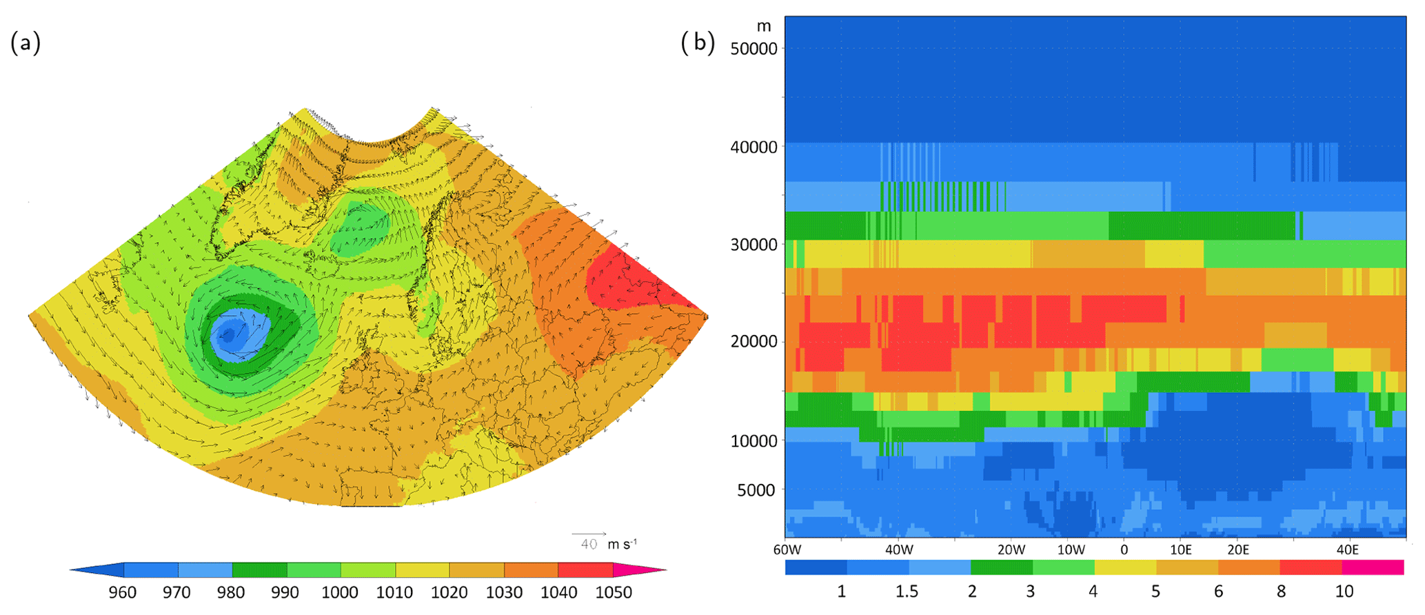
Figure 1(a) Mean sea level (MSL) pressure (colour shades, hPa) and wind at ∼ 1830 m a.s.l. (eighth hybrid model level, vectors, m s−1) at 12:00 UTC on 2 November 2018; (b) vertical ozone concentration profiles (µmol m−3) at latitude 62∘ N at 12:00 on 4 November 2018.
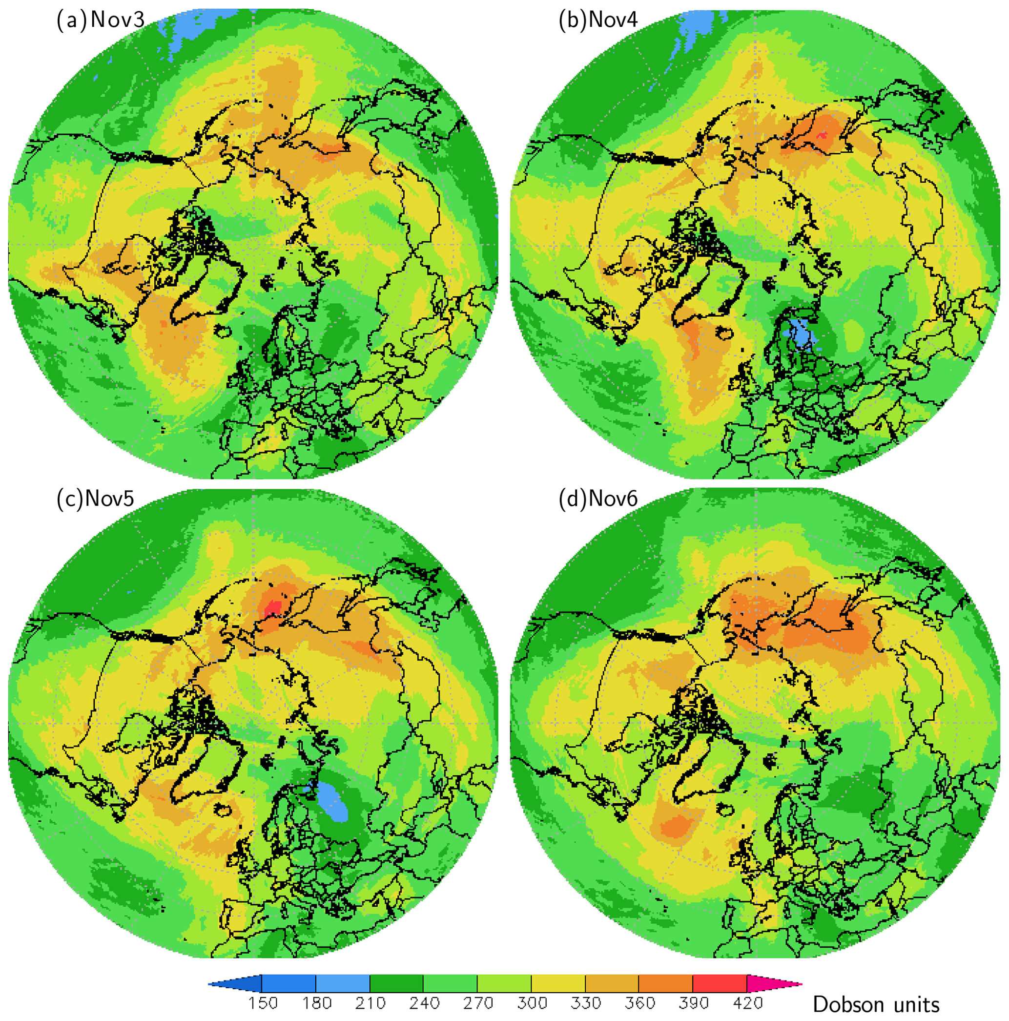
Figure 2Midday (UTC time) total ozone column in DU (Dobson units) for 3–6 November 2018 as predicted by the SILAM model on 1 November 2018. Forecast lengths were from +59 for (a) until +131 h for (d).
3.2 Evaluation of the SILAM predictions
Evaluation of the above model predictions was performed against OMI and OMPS satellite retrievals of the ozone total column, as well as against MLS–HARMOZ vertical ozone profiles. Due to very similar patterns shown by both nadir satellites, below we discuss the OMI-based comparison. The focus was on the model ability to reproduce the absolute level of the ozone column load, as well as on accurate location of the depletion area in space and time.
The model predictions, namely the shape and evolution of the low-ozone area over Scandinavia, were confirmed (Fig. 3 for 4 November 2018 and Figs. S8–S13 for the whole period). The only issue revealed by the comparison was a quite homogeneous underestimation of the total ozone column by SILAM – within 10–20 DU over the bulk of the domain (Fig. 3). This bias was also stable in time and practically did not vary throughout the episode (see the Supplement); i.e. the anomaly of the ozone column was predicted with <10 DU error, its location was accurate within ∼100 km, and timeliness was captured with <1 d accuracy. Accounting for this bias, the actual ozone load was about 210–215 DU at the peak of the episode (whereas SILAM suggested it down to 200 DU), compared to ∼ 310–320 DU of a zonal-mean level between 60 and 80∘ N excluding the depletion area (the corresponding SILAM mean was about 300 DU).
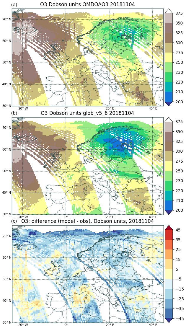
Figure 3Daily-composite ozone column (DU) for 4 November 2018 observed by OMI DOAS (a) and predicted by SILAM (b). Only grid cells corresponding to valid OMI observations were retained in the SILAM forecast. (c) Difference of modelled minus observed ozone column (DU).
Considering the S1–S7 and the corresponding S8–S13 figures, one can notice that the underestimation of the ozone column load was somewhat stronger in the tropics than in the northern regions. This has been traced to the very low lightning emission of NO2 in the input files and too intense scavenging of tropospheric ozone precursors. These resulted in low tropospheric ozone concentrations in the tropical regions, thus adding ∼5 DU of the underestimation of the total column. However, these effects do not concern the current case and have been rectified in the new SILAM v.5.7 that will be put in operation in 2020.
The vertical distribution of the ozone loss on 4 November 2018 was predicted to span up to 25 km and beyond (Fig. 1b). A similar effect is also seen in the MLS retrievals (Fig. 4), which show that the highest ozone concentrations during the episode were predicted and observed at 22–23 km instead of the usual 17–18 km. The absolute concentrations at that altitude however changed just a bit going slightly below 7 µmol m−3 (Fig. 4b) instead of 7.5 µmol m−3 as the median level over the latitude belt outside the depletion area. One can also see that the bulk of ozone reduction occurred between the 5 and 23 km altitude levels, but even above the 25 km level the concentrations were in the lower quartile of the 60–80∘ N belt. This is well in agreement with the SILAM forecasts (Fig. 4) and confirms an unusually strong penetration of the tropospheric air into the stratosphere. The only noticeable disagreement between SILAM and MLS was around 15–18 km altitude, where SILAM predicted concentrations about half a micromole per cubic metre lower than reported by MLS, i.e. underestimated by ∼25 %. However, the uncertainty of this bias is 2 times larger than its absolute value, which might be explained by MLS approaching the lower end of the observed altitude range. The altitude of 10 km was reached by only few MLS profiles, which nevertheless showed very good agreement.
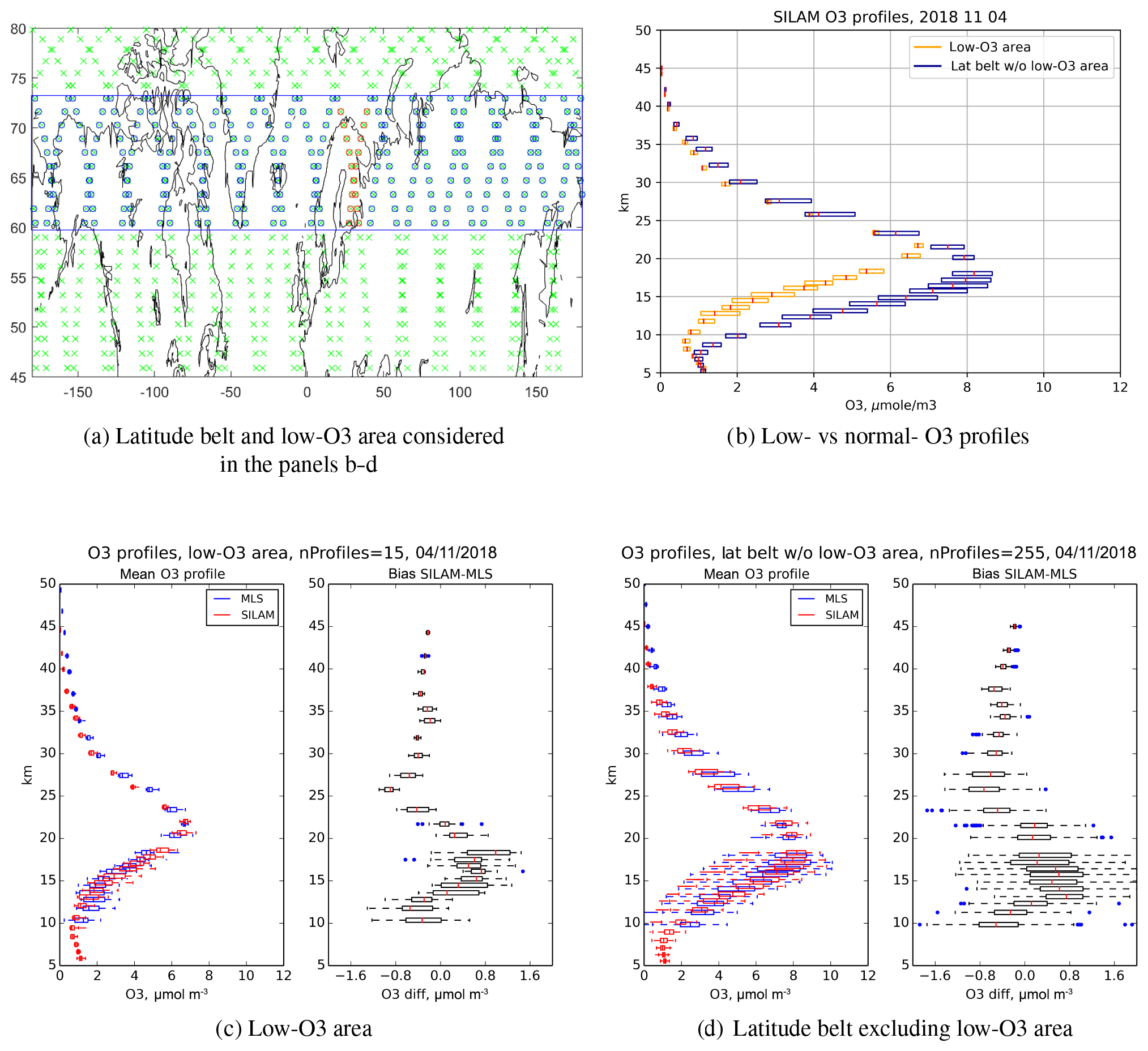
Figure 4(a) Locations of the MLS ozone profiles on 4 November 2018; the latitude belt 59–74∘ N and the longitudinal range 20–40∘ E (low-O3 area) are highlighted. (b) SILAM O3 vertical profiles predicted within and outside of the low-O3 area; (c) MLS and SILAM ozone vertical profiles and their difference in the low-O3 area; (d) same as (c) but for rest of the latitude belt excluding the low-O3 area. SILAM boxes in (c) and (d) are shifted upwards by 0.4 km in order to prevent overlapping pictures.
As mentioned in the methodological Sect. 2, the SILAM global forecasts are performed without observational data assimilation; i.e. the next forecast is started from the appropriate time step of the previous one. At a price of certain worsening of the formal scores, such as the model bias at some altitudes, this approach ensures well-balanced simulations: the quality of the forecast deteriorates only slightly over the whole predicted period (see the Supplement). The connection to reality is ensured by the meteorological driver IFS, which assimilates the meteorological observations at the start of each forecast.
Looking into history of the OMI observations, the current episode was quite extreme, although not record setting. In its depth on 4 November 2018, it corresponded to the 0.5th percentile of the ozone distribution in November north of 60∘ N observed by OMI over the 12-year period of operations (2005–2017). Its strength was a result of coincidence of otherwise normal phenomena: storm in the northern Atlantic creating the initial WCB uplift, eastwards air mass transport over the Scandinavian ridge with additional rise, and low solar radiation in November delaying the ozone recovery. Only three episodes, also in November (the month with the lowest ozone load in the northern subpolar areas), during these 12 years were stronger. The deepest decline in the subpolar region in November was in 2009 (the observed column load was below 180 DU) followed by 2008 with minimum observed column just over 180 DU, also spanning a large area (Fig. S14). An interesting month was also November of 2012 when the median level of column load was at 300 DU instead of the usual 320 DU. No evident trend in the median or minimum column loads in November in northern subpolar latitudes was found over these years.
The overall impact of the considered episode on the large-scale atmospheric processes was small due to its intermittent limited-area character. The reduction of the ozone amount at 12:00 4 November 2018 in comparison with the “unperturbed” level was 1.3 Tg, which is almost 30 % of the layer over Finland but just 0.6 % of the total ozone amount in the 60–80∘ N belt (205 Tg, as predicted by SILAM). However, one has to keep in mind that during the stormy autumn–winter months quite a few cyclones have the capacity to create such depletion events.
From a health prospective, the low UV level in November in northern latitudes precluded any significant impact. For the future, the projected increase in the strength of storms can potentially make the tropospheric intrusions more significant players than the current episode.
Climate change will probably increase the strength and frequency of such events but quantitative assessment is difficult. Indeed, as shown above, such episodes are started by strong storms. Numerous studies summarized in IPCC Assessment Report AR5 and the special report “Global Warming of 1.5∘” showed that there is a general tendency of a decreasing global number of tropical cyclones and accumulated cyclonic energy (e.g. Elsner et al., 2008; Knutson et al., 2010; Hoegh-Guldberg et al., 2018, and references therein). The phenomenon has also been understood from theoretical point of view (Kang and Elsner, 2015). According to these findings and future-climate projections, further decrease in cyclonic activity is likely. However, IPCC assigned low confidence to this conclusion due to several studies reporting contradicting trends. At the same time, the number and intensity of severe cyclones and storms has increased and will probably increase further (also with low confidence according to IPCC) (Knutson et al., 2013). The latter expectation is supported by, for example, statistics of strong storms in the Atlantic (includes the whole of the Atlantic), which shows that the number of major named storms has grown from seven per year in the 1850s to 13 in the 2010s (http://www.stormfax.com/huryear.htm, last access: 16 August 2019). The sharp growth started around 1990, adding almost 30 % within the last 30 years. Since the intermittent ozone holes will be associated with strong storms, one can expect an increase in both frequency and strength of such events in the future.
An episode of a strong tropospheric intrusion into the UTLS and to the middle stratosphere was predicted by the SILAM model and subsequently observed by the ozone monitoring satellites at the beginning of November 2018. According to the model predictions, the intrusion resulted in a short (∼ 3 d) but significant (30 %, from >300 down to ∼200 DU) regional reduction of the total ozone column. The most-significant reduction occurred over northern Scandinavia, owing to an additional enforcement of the intrusion by the lift-up over the Scandinavian ridge.
Satellite observations of the total ozone column (OMI and OMPS) and ozone profiles (MLS) confirmed both the temporal development (within <1 d, which corresponds to frequency of the satellite overpasses) and the spatial location of the depletion event. Absolute level of the total ozone column has been homogeneously underestimated by ∼20 DU, both within and outside of the depletion area, partially due to the very low NO2 emission of lightning and somewhat too strong scavenging of ozone precursors in the troposphere. Prediction of the ozone column anomaly was within ∼10 DU.
The episode corresponded to the 0.5th percentile of the OMI observations over the period 2005–2017 for the latitude belt 60–80∘ N in November (the month with the lowest ozone concentration in the northern subpolar stratosphere). Despite the comparatively extreme character of the episode, its impact on the large-scale atmospheric processes and UV index at the surface was small due to the intermittent character of the ozone reduction and the low level of UV radiation in northern Europe in November. However, significance of the phenomenon can grow in the future due to an increasing number of strong storms in the northern Atlantic.
High accuracy of the episode prediction 5 d in advance by the IFS–SILAM system shows the possibility of prediction of details of stratospheric composition and its short-term dynamics, including such rare events.
The SILAM forecasts are openly available from http://silam.fmi.fi/aqforecast.html (Sofiev et al., 2020) as a week-long rolling archive. Due to large size (>2 TB d−1), only a subset of the forecasts is archived over the long term. That information is available on request from the authors of the paper.
SILAM is an open-code system and can be obtained from the GitHub open repository (https://github.com/fmidev/silam-model, Kouznetsov and Delgado, 2020) or from the authors of the paper.
The supplement related to this article is available online at: https://doi.org/10.5194/acp-20-1839-2020-supplement.
MS performed the analysis of the operational forecasts and wrote the paper; RK configured the operational forecasts and participated in the analysis and writing; RH developed the new chemistry transformation scheme and participated in writing; VFS performed the satellite data analysis and participated in writing.
The authors declare that they have no conflict of interest.
The SILAM stratospheric modules were developed within the Finnish Academy ASTREX project (grant no. 139126). The work has been performed within the GLORIA project of the Academy of Finland (grant no. 310373). Support from the ESA SUNLIT and H2020 AirQast (grant no. 776361) projects is kindly appreciated.
This research has been supported by the Academy of Finland (grant nos. 310373 and 139126), the European Space Agency (SUNLIT project), and the Horizon 2020 Framework Programme (AirQast (grant no. 776361)).
This paper was edited by Michel Van Roozendael and reviewed by three anonymous referees.
Carslaw, K. S., Luo, B., and Peter, T.: An analytic expression for the composition of aqueous HNO3-H2SO4 stratospheric aerosols including gas phase removal of HNO3, Geophys. Res. Lett., 22, 1877–1880, 1995.
Cunnold, D. M., Fraser, P. J., Weiss, R. F., Prinn, R. G., Simmonds, P. G., Miller, B. R., Alyea, F. N., and Crawford, A. J.: Global trends and annual releases of CCl3F and CCl2F2 estimated from ALE/GAGE and other measurements from July 1978 to June 1991, J. Geophys. Res., 99, 1107, https://doi.org/10.1029/93JD02715, 1994.
Damski, J., Thölix, L., Backman, L., Taalas, P., and Kulmala, M.: FinROSE: middle atmospheric chemistry transport model, Boreal Environ. Res., 12, 535–550, 2007.
Ebel, A., Hass, H., Jakobs, H., Laube, M., Memmesheimer, M., Oberreuter, A., Geiss, H., and Kuo, Y.-H.: Simulation of ozone intrusion caused by tropopause fold and COL, Atmos. Environ. A-Gen., 25, 2131–2144, https://doi.org/10.1016/0960-1686(91)90089-P, 1991.
Edwards, P. M. and Evans, M. J.: A new diagnostic for tropospheric ozone production, Atmos. Chem. Phys., 17, 13669–13680, https://doi.org/10.5194/acp-17-13669-2017, 2017.
Elsner, J. B., Kossin, J. P., and Jagger, T. H.: The increasing intensity of the strongest tropical cyclones, Nat. Clim. Change, 455, 2–5, https://doi.org/10.1038/nature07234, 2008.
Flynn, L. E., Seftor, C. J., Larsen, J. C., and Xu, P.: The Ozone Mapping and Profiler Suite, in: Earth Science Satellite Remote Sensing: Vol. 1: Science and Instruments, edited by: Qu, J. J., Gao, W., Kafatos, M., Murphy, R. E., and Salomonson, V. V., 279–296, Springer Berlin Heidelberg, Berlin, Heidelberg, 2006.
Gery, M. W., Whitten, G. Z., Killus, J. P., and Dodge, M. C.: A photochemical kinetics mechanism for urban and regional scale computer modeling, J. Geophys. Res., 94, 12925–12956, 1989.
Granier, C., Bessagnet, B., Bond, T., D'Angiola, A., Denier van der Gon, H., Frost, G. J., Heil, A., Kaiser, J. W., Kinne, S., Klimont, Z., Kloster, S., Lamarque, J.-F., Liousse, C., Masui, T., Meleux, F., Mieville, A., Ohara, T., Raut, J.-C., Riahi, K., Schultz, M. G., Smith, S. J., Thompson, A., Aardenne, J., Werf, G. R., and Vuuren, D. P.: Evolution of anthropogenic and biomass burning emissions of air pollutants at global and regional scales during the 1980–2010 period, Climatic Change, 109, 163–190, https://doi.org/10.1007/s10584-011-0154-1, 2011.
Hoegh-Guldberg, O., Jacob, D., Taylor, M., Bindi, M., Brown, S., Camilloni, I., Diedhiou, A., Djalante, R., Ebi, K. L., Engelbrecht, F., Guiot, J., Hijioka, Y., Mehrotra, S., Payne, A., Seneviratne, S. I., Thomas, A., Warren, R., and Zhou, G.: Impacts of 1.5 ∘C Global Warming on Natural and Human Systems, in: Global Warming of 1.5 ∘C, IPCC Special Report on the impacts of global warming of 1.5 ∘C above pre-industrial levels and related global greenhouse gas emission pathways, in the context of strengthening the global response to the threat of climate change, sustainable development, p. 138, IPCC, Switzerland, 2018.
Jaeglé, L., Wood, R., and Wargan, K.: Multiyear Composite View of Ozone Enhancements and Stratosphere-to-Troposphere Transport in Dry Intrusions of Northern Hemisphere Extratropical Cyclones, J. Geophys. Res.-Atmos., 122, 13436–13457, https://doi.org/10.1002/2017JD027656, 2017.
Jalkanen, J.-P., Brink, A., Kalli, J., Pettersson, H., Kukkonen, J., and Stipa, T.: A modelling system for the exhaust emissions of marine traffic and its application in the Baltic Sea area, Atmos. Chem. Phys., 9, 9209–9223, https://doi.org/10.5194/acp-9-9209-2009, 2009.
Jalkanen, J.-P., Johansson, L., and Kukkonen, J.: A comprehensive inventory of ship traffic exhaust emissions in the European sea areas in 2011, Atmos. Chem. Phys., 16, 71–84, https://doi.org/10.5194/acp-16-71-2016, 2016.
Kaiser, J. W., Suttie, M., Flemming, J., Morcrette, J.-J., Boucher, O., Schultz, M. G., Nakajima, T., and Yamasoe, M. A.: Global Real-time Fire Emission Estimates Based on Space-borne Fire Radiative Power Observations, AIP Conf. Proc., 1100, 645–648, https://doi.org/10.1063/1.3117069, 2009.
Kang, N. and Elsner, J. B.: Trade-o between intensity and frequency of global tropical cyclones, Nat. Clim. Change, 5, 661–664, https://doi.org/10.1038/NCLIMATE2646, 2015.
Knutson, T. R., McBride, J. L., Chan, J., Emanuel, K., Holland, G., Landsea, C., Held, I., Kossin, J. P., Srivastava, A. K., and Sugi, M.: Tropical cyclones and climate change, Nat. Geosci., 3, 157–163, https://doi.org/10.1038/ngeo779, 2010.
Knutson, T. R., Sirutis, J. J., Vecchi, G. A., Garner, S., Zhao, M., Kim, H.-S., Bender, M., Tuleya, R. E., Held, I. M., and Villarini, G.: Dynamical Downscaling Projections of Twenty-First-Century Atlantic Hurricane Activity?: CMIP3 and CMIP5 Model-Based Scenarios, J. Climate, 26, 6591–6617, https://doi.org/10.1175/JCLI-D-12-00539.1, 2013.
Kouznetsov, R. and Delgado, R.: SILAM open code at GitHub, available at: https://github.com/fmidev/silam-model, last access: 10 February 2020.
Lee, D. S., Pitari, G., Grewe, V., Gierens, K., Penner, J. E., Pet-zold, A., Prather, M. J., Schumann, U., Bais, A., Berntsen, T., Iachetti, D., Lim, L. L., and Sausen, R.: Transport impacts onatmosphere and climate: aviation, Atmos. Environ., 44, 4678–4734, https://doi.org/10.1016/j.atmosenv.2009.06.005, 2009
Levelt, P. F., van den Oord, G. H. J., Dobver, M. R., Mälkki, A., Visser, H., de Vries, J., Stammes, P., Lundell, J. O. V., and Saari, H.: The ozone monitoring instrument, IEEE T. Geosci. Remote Sens., 44, 1093–1101, https://doi.org/10.1109/TGRS.2006.872333, 2006.
Levelt, P. F., Joiner, J., Tamminen, J., Veefkind, J. P., Bhartia, P. K., Stein Zweers, D. C., Duncan, B. N., Streets, D. G., Eskes, H., van der A, R., McLinden, C., Fioletov, V., Carn, S., de Laat, J., DeLand, M., Marchenko, S., McPeters, R., Ziemke, J., Fu, D., Liu, X., Pickering, K., Apituley, A., González Abad, G., Arola, A., Boersma, F., Chan Miller, C., Chance, K., de Graaf, M., Hakkarainen, J., Hassinen, S., Ialongo, I., Kleipool, Q., Krotkov, N., Li, C., Lamsal, L., Newman, P., Nowlan, C., Suleiman, R., Tilstra, L. G., Torres, O., Wang, H., and Wargan, K.: The Ozone Monitoring Instrument: overview of 14 years in space, Atmos. Chem. Phys., 18, 5699–5745, https://doi.org/10.5194/acp-18-5699-2018, 2018.
Lobert, J. M., Keene, W. C., Logan, J. A., and Yevich, R.: Global chlorine emissions from biomass burning?: Reactive Chlorine Emissions Inventory, J. Geophys. Res., 104, 8373–8389, 1999.
Olsen, M. A., Douglass, A. R., and Kaplan, T. B.: Variability of extratropical ozone stratosphere–troposphere exchange using microwave limb sounder observations, J. Geophys. Res.-Atmos., 118, 1090–1099, https://doi.org/10.1029/2012JD018465, 2013.
Orbe, C., Waugh, D. W., and Newman, P. A.: Air-mass origin in the tropical lower stratosphere: The influence of Asian boundary layer air, Geophys. Res. Lett., 42, 4240–4248, https://doi.org/10.1002/2015GL063937, 2015.
Pan, L. L., Randel, W. J., Gille, J. C., Hall, W. D., Nardi, B., Massie, S., Yudin, V., Khosravi, R., Konopka, P., and Tarasick, D.: Tropospheric intrusions associated with the secondary tropopause, J. Geophys. Res., 114, D10302, https://doi.org/10.1029/2008JD011374, 2009.
Price, C., Penner, J., and Prather, M.: NOx from lightning: 1. Global distribution based on lightning physics, J. Geophys. Res., 102, 5929, https://doi.org/10.1029/96JD03504, 1997.
Reutter, P., Škerlak, B., Sprenger, M., and Wernli, H.: Stratosphere–troposphere exchange (STE) in the vicinity of North Atlantic cyclones, Atmos. Chem. Phys., 15, 10939–10953, https://doi.org/10.5194/acp-15-10939-2015, 2015.
Roelofs, G. and Lelieveld, J.: Tropospheric ozone simulation with a chemistry-general circulation model?: Influence of higher hydrocarbon chemistry, J. Geophys. Res.-Atmos., 105, 22697–22712, https://doi.org/10.1029/2000JD900316, 2000.
Sindelarova, K., Granier, C., Bouarar, I., Guenther, A., Tilmes, S., Stavrakou, T., Müller, J.-F., Kuhn, U., Stefani, P., and Knorr, W.: Global data set of biogenic VOC emissions calculated by the MEGAN model over the last 30 years, Atmos. Chem. Phys., 14, 9317–9341, https://doi.org/10.5194/acp-14-9317-2014, 2014.
Sofiev, M.: A model for the evaluation of long-term airborne pollution transport at regional and continental scales, Atmos. Environ., 34, 2481–2493, 2000.
Sofiev, M., Vankevich, R., Lotjonen, M., Prank, M., Petukhov, V., Ermakova, T., Koskinen, J., and Kukkonen, J.: An operational system for the assimilation of the satellite information on wild-land fires for the needs of air quality modelling and forecasting, Atmos. Chem. Phys., 9, 6833–6847, https://doi.org/10.5194/acp-9-6833-2009, 2009.
Sofiev, M., Soares, J., Prank, M., Leeuw, G., and Kukkonen, J.: A regional-to-global model of emission and transport of sea salt particles in the atmosphere, J. Geophys. Res., 116, D21302, https://doi.org/10.1029/2010JD014713, 2011.
Sofiev, M., Vankevich, R., Ermakova, T., and Hakkarainen, J.: Global mapping of maximum emission heights and resulting vertical profiles of wildfire emissions, Atmos. Chem. Phys., 13, 7039–7052, https://doi.org/10.5194/acp-13-7039-2013, 2013.
Sofiev, M., Vira, J., Kouznetsov, R., Prank, M., Soares, J., and Genikhovich, E.: Construction of the SILAM Eulerian atmospheric dispersion model based on the advection algorithm of Michael Galperin, Geosci. Model Dev., 8, 3497–3522, https://doi.org/10.5194/gmd-8-3497-2015, 2015.
Sofiev, M., Winebrake, J. J., Johansson, L., Carr, E. W., Prank, M., Soares, J., Vira, J., Kouznetsov, R., Jalkanen, J.-P., and Corbett, J. J.: Cleaner fuels for ships provide public health benefits with climate tradeoffs, Nat. Commun., 9, 406, https://doi.org/10.1038/s41467-017-02774-9, 2018.
Sofiev, M., Kouznetsov, R., Vira, J., Hanninen, R., Uppstu, A., and Braznov, T.: SILAM Web site, available at: http://silam.fmi.fi/aqforecast.html, last access: 13 February 2020.
Sofieva, V. F., Rahpoe, N., Tamminen, J., Kyrölä, E., Kalakoski, N., Weber, M., Rozanov, A., von Savigny, C., Laeng, A., von Clarmann, T., Stiller, G., Lossow, S., Degenstein, D., Bourassa, A., Adams, C., Roth, C., Lloyd, N., Bernath, P., Hargreaves, R. J., Urban, J., Murtagh, D., Hauchecorne, A., Dalaudier, F., van Roozendael, M., Kalb, N., and Zehner, C.: Harmonized dataset of ozone profiles from satellite limb and occultation measurements, Earth Syst. Sci. Data, 5, 349–363, https://doi.org/10.5194/essd-5-349-2013, 2013.
Stohl, A.: A 1-year Lagrangian “climatology” of airstreams in the Northern Hemisphere troposphere and lowermost stratosphere, J. Geophys. Res.-Atmos., 106, 7263–7279, https://doi.org/10.1029/2000JD900570, 2001.
Stohl, A.: Stratosphere-troposphere exchange: A review, and what we have learned from STACCATO, J. Geophys. Res., 108, 8516, https://doi.org/10.1029/2002jd002490, 2003.
Waters, J. W., Froidevaux, L., Harwood, R. S., Jarnot, R. F., Pickett, H. M., Read, W. G., Siegel, P. H., Cofield, R. E., Filipiak, M. J., Flower, D. A., Holden, J. R., Lau, G. K. K., Livesey, N. J., Manney, G. L., Pumphrey, H. C., Santee, M. L., Wu, D. L., Cuddy, D. T., Lay, R. R., Loo, M. S., Perun, V. S., Schwartz, M. J., Stek, P. C., Thurstans, R. P., Boyles, M. A., Chandra, K. M., Chavez, M. C., Chen, G. S., Chudasama, B. V, Dodge, R., Fuller, R. A., Girard, M. A., Jiang, J. H., Jiang, Y. B., Knosp, B. W., LaBelle, R. C., Lam, J. C., Lee, K. A., Miller, D., Oswald, J. E., Patel, N. C., Pukala, D. M., Quintero, O., Scaff, D. M., Van Snyder, W., Tope, M. C., Wagner, P. A., and Walch, M. J.: The Earth Observing System Microwave Limb Sounder (EOS MLS) on the Aura satellite, IEEE T. Geosci. Remote Sens., 44, 1075–1092, https://doi.org/10.1109/TGRS.2006.873771, 2006.