the Creative Commons Attribution 4.0 License.
the Creative Commons Attribution 4.0 License.
 | 04 Feb 2020
Variability of hydroxyl radical (OH) reactivity in the Landes maritime pine forest: results from the LANDEX campaign 2017
Sandy Bsaibes
Mohamad Al Ajami
Kenneth Mermet
François Truong
Sébastien Batut
Christophe Hecquet
Sébastien Dusanter
Thierry Léornadis
Stéphane Sauvage
Julien Kammer
Pierre-Marie Flaud
Emilie Perraudin
Eric Villenave
Nadine Locoge
Valérie Gros
Coralie Schoemaecker
Total hydroxyl radical (OH) reactivity measurements were conducted during the LANDEX intensive field campaign in a coniferous temperate forest located in the Landes area, southwestern France, during July 2017. In order to investigate inter-canopy and intra-canopy variability, measurements were performed inside (6 m) and above the canopy level (12 m), as well as at two different locations within the canopy, using a comparative reactivity method (CRM) and a laser photolysis–laser-induced fluorescence (LP-LIF) instrument. The two techniques were intercompared at the end of the campaign by performing measurements at the same location. Volatile organic compounds were also monitored at both levels with a proton transfer time-of-flight mass spectrometer and online gas chromatography instruments to evaluate their contribution to total OH reactivity, with monoterpenes being the main reactive species emitted in this forest dominated by Pinus pinaster Aiton. Total OH reactivity varied diurnally, following the trend of biogenic volatile organic compounds (BVOCs), the emissions and concentrations of which were dependent on meteorological parameters. Average OH reactivity was around 19.2 and 16.5 s−1 inside and above the canopy, respectively. The highest levels of total OH reactivity were observed during nights with a low turbulence ( m s−1), leading to lower mixing of emitted species within the canopy and thus an important vertical stratification characterized by a strong concentration gradient. Comparing the measured and the calculated OH reactivity highlighted an average missing OH reactivity of 22 % and 33 % inside and above the canopy, respectively. A day–night variability was observed on missing OH reactivity at both heights. Investigations showed that during daytime, missing OH sinks could be due to primary emissions and secondary products linked to a temperature-enhanced photochemistry. Regarding nighttime missing OH reactivity, higher levels were seen for the stable and warm night of 4–5 July, showing that these conditions could have been favorable for the accumulation of long-lived species (primary and secondary species) during the transport of the air mass from nearby forests.
- Article
(5954 KB) - Full-text XML
-
Supplement
(1706 KB) - BibTeX
- EndNote


The hydroxyl radical (OH) is considered the most important initiator of photochemical processes in the troposphere during daytime and the prevailing “detergent” from local to global scales. It controls the lifetime of most trace gases and contributes to the self-cleansing power or so-called “oxidation capacity” of the atmosphere.
Even though the main primary source for OH in the lower troposphere is the photolysis of ozone at short wavelengths, the OH production and loss processes are numerous and difficult to quantify. Such losses involve several hundred chemical species and as many reactions to consider. In this respect, a direct measurement of total OH reactivity (ROH) is of great interest to better understand the OH chemistry in the atmosphere and to investigate the budget of OH sinks in a particular environment. ROH is defined as the pseudo-first-order loss rate (s−1) of OH radicals, equivalent to the inverse of the OH lifetime. It is the sum of the reaction frequencies of all chemical species reacting with OH, as shown in Eq. (1):
In this equation, a chemical reaction frequency for a species Xi with OH () is the product of its rate coefficient kOH with its concentration [Xi]. The measured total OH reactivity can be compared with calculated values based on the sum of reaction frequencies as shown in Eq. (1) and for which the concentration of Xi has been measured at the same location. Any significant discrepancy between measured and calculated OH reactivity explicitly demonstrates missing OH sinks, commonly called missing OH reactivity, and points out that potentially important unmeasured reactive species and chemical processes associated with these species may affect our understanding of OH atmospheric chemistry.
Two approaches have been used to measure total OH reactivity. The first approach derives OH reactivity from direct measurements of OH decay rates due to its reaction with the trace species present in ambient air introduced in a reaction tube. OH can be generated and detected differently according to three types of techniques: flow tube laser-induced fluorescence (FT-LIF; Hansen et al., 2014; Ingham et al., 2009; Kovacs and Brune, 2001), laser photolysis–laser-induced fluorescence (LP-LIF; Sadanaga et al., 2004; Parker et al., 2011; Amedro et al., 2012; Stone et al., 2016; Fuchs et al., 2017) and flow tube chemical-ionization mass spectrometry (FT-CIMS; Muller et al., 2018). The second approach is called the comparative reactivity method (CRM), and it consists of an indirect quantification of OH losses from the concentration change of a reference molecule that competes with ambient reactive species to react with artificially produced OH. The reference substance, pyrrole, is measured with a proton transfer reaction mass spectrometer (PTR-MS; Sinha et al., 2008; Dolgorouky et al., 2012; Michoud et al., 2015), with a gas chromatograph–photoionization detector (GC-PID; Nölscher et al., 2012) or with chemical ionization mass spectrometry (CIMS; Sanchez et al., 2018).
Both LP-LIF and CRM techniques were deployed in a pine forest for this study; the instruments deployed are presented in more detail below and a general description is provided here. In the LP-LIF method, OH is generated by the laser-pulsed photolysis of ozone in a reaction tube, typically at 266 nm, followed by the rapid reaction of O(1D) with ambient water vapor. OH radicals react with ambient reactive species in the reaction tube and the concentration of OH decreases after the laser pulse. The air from the reaction tube is continuously pumped into a low-pressure detection cell where the OH decay is monitored by laser-induced fluorescence at a high time resolution (range of hundreds of microseconds) (Sadanaga et al., 2004). Compared to flow tube setups, lower flow rates of ambient air are needed in the LP-LIF technique (less than 10 L min−1 compared to several tens of liters per minute). In addition, the use of O3 laser photolysis instead of continuous water photolysis by lamps at 185 nm for OH generation, the latter being commonly used in FT-LIF and CRM, limits the spurious formation of OH from the reaction of HO2 with ambient NO. However, in order to quantify wall loss reactions, an instrument zero has to be subtracted from all measurements, and a correction may have to be applied for the recycling of OH radicals in the presence of high NO levels (Stone et al., 2016; Fuchs et al., 2017).
In the comparative reactivity method (CRM), ambient air, wet nitrogen and pyrrole are introduced into a glass reactor where OH radicals are produced by the photolysis of water vapor. The mathematical expression used to determine the OH reactivity of the analyzed sample is derived in terms of the initial concentration of pyrrole (C1), the background concentration of pyrrole reacting alone with OH (C2) and the concentration of pyrrole after competition with air reactants (C3). The CRM exhibits several advantages compared to direct measurements techniques, like the commercial availability of PTR-MS and the need for a smaller sampling flow rate of ambient air (a few hundred milliliters per minute), which broadens the application of the technique to branch and plant enclosure studies. On the other hand, this indirect method requires a raw data processing with careful corrections for measurement artifacts related to humidity changes and secondary chemistry that can impact the pyrrole concentration (Sinha et al., 2008; Michoud et al., 2015).
A few intercomparisons were reported in the literature for urban and remote areas (Hansen et al., 2015; Zannoni, 2015; Sanchez et al., 2018) as well as in chamber experiments (Fuchs et al., 2017) aiming at reproducing the ambient conditions observed in various environments. The latter, including a large number of OH reactivity instruments (FT-LIF, LP-LIF, CRM) for studies conducted in the SAPHIR atmospheric simulation chamber, allowed for a comparison of the performances of each technique. Results showed that OH reactivity can be accurately measured for a wide range of atmospherically relevant chemical conditions by all instruments. However, CRM instruments exhibited larger discrepancies with calculated OH reactivity compared to instruments directly probing OH radicals, and these differences were more important in the presence of terpenes and oxygenated organic compounds.
Over the past 2 decades, OH reactivity measurements have been conducted in various environments at the ground level using the available techniques: urban and suburban areas, forest areas, and marine areas (Yang et al., 2016; Dusanter and Stevens, 2017). A few aircraft measurements have also been carried out to complete ground-based observations (Brune et al., 2010). Many studies highlighted the interest of investigating OH reactivity in forest areas exhibiting large concentrations of biogenic volatile organic compounds (BVOCs) since BVOC emissions exceed anthropogenic VOCs by a factor of 10 at the global scale (Guenther et al., 1995). Results showed that our understanding of OH sinks in these environments was incomplete, with observations of large missing OH reactivity ranging between 25 % and 80 %. Total OH reactivity appeared to be impacted by several factors such as the forest type and the dominant emitted species, the seasonality, the canopy level, and specific atmospheric conditions (Hansen et al., 2014; Nölscher et al., 2013; Praplan et al., 2019; Sanchez et al., 2018; Zannoni et al., 2016).
Among these biogenic hydrocarbons, monoterpenes represent a large class of C10H16 compounds, which are mainly emitted by conifers as well as broad-leaved trees. They can be oxidized by OH, ozone and the nitrate radical, leading to atmospheric lifetimes ranging between minutes and days (Atkinson and Arey, 2003). The oxidation of primary BVOCs can therefore contribute to the formation of tropospheric ozone and secondary organic aerosols from local to the regional scales, with the oxidation products of BVOCs having a potential impact at a larger scale. Regarding coniferous forests, an averaged OH reactivity of 6.7 s−1 was observed over a temperate pine forest located in the southern part of the Rocky Mountains in the USA during summer 2008 (Nakashima et al., 2013). Measured OH reactivity exhibited a diurnal variation, with minima during daytime when MBO (2-methyl-3-buten-2-ol) was the main contributor and maxima during nighttime when the OH reactivity was dominated by monoterpenes. Approximately 30 % of the measured OH reactivity remained unexplained and could be related to unmeasured or unknown oxidation products of primary emitted biogenic compounds. Another campaign also carried out in a temperate coniferous forest, located in the Wakayama Forest Research Station in Japan during summer 2014 (Ramasamy et al., 2016), showed comparable results with an average total OH reactivity of 7.1 s−1. OH reactivity varied diurnally with temperature and light, reaching a maximum at noontime. Monoterpenes were the main drivers of the total OH reactivity in the considered ecosystem, accounting for 23.7 %, followed by isoprene (17.0 %) and acetaldehyde (14.5 %). The missing OH reactivity (29.5 % on average) was found to be linked to light- and temperature-dependent unmeasured primary and secondary species.
In the present study, we report on the measurement of total OH reactivity from a field experiment conducted in the Landes temperate forest, southwestern France. This work was part of the LANDEX project (LANDEX, i.e., the Landes Experiment: Formation and fate of secondary organic aerosols generated in the Landes forest) that aimed to characterize secondary organic aerosol formation observed in this monoterpene-rich environment. The dominant tree species at the site is maritime pine, Pinus pinaster Aiton, which is known to be a strong emitter of α- and β-pinene, leading to a diurnal concentration profile of monoterpenes characterized by maximum values at night and minimum values during daytime (Simon et al., 1994). Nocturnal new particle formation episodes (NPFs) were reported in this ecosystem, suggesting the contribution of BVOC oxidation to the nucleation and growth stages of particles (Kammer et al., 2018).
Measurements of OH reactivity and trace gases were performed at two heights to cover inside and above the canopy, as well as at two different locations inside the canopy to investigate the intra-canopy variability. Two different instruments were deployed: the CRM from LSCE (Laboratoire des Sciences du Climat et de l'Environnement), which measured inside and above the canopy, and the LP-LIF from PC2A (Laboratoire PhysicoChimie des Processus de Combustion et de l'Atmosphère) that performed measurements inside the canopy. The deployment of two different instruments was a good opportunity to (i) compare measurements made with both methods in a real biogenic environment after the intercomparison experiment performed in the SAPHIR chamber and recent improvement of the CRM instrument, (ii) investigate the levels and diurnal variability of OH reactivity at two different heights, and (iii) investigate both the OH reactivity budget and the missing reactivity pattern using a large panel of concomitant trace gas measurements.
2.1 Site description
The LANDEX intensive field campaign was conducted from 3 to 19 July 2017 at the Bilos field site in the Landes forest, southwestern France. The vegetation on the site was dominated by maritime pines (Pinus pinaster Aiton) presenting an average height of 10 m. The climate is temperate with a maritime influence due to the proximity of the Atlantic Ocean. This site is part of the European ICOS (Integrated Carbon Observation System) ecosystem infrastructure. A more detailed description of the site is available in Moreaux et al. (2011) and Kammer et al. (2018).
2.2 OH reactivity instruments
The LP-LIF instrument, referred to here as UL-FAGE (University of Lille-FAGE – Fluorescence Assay by Gas Expansion), measured the OH reactivity in the canopy, whereas the CRM instrument, referred to as LSCE-CRM, alternatively measured the OH reactivity at two heights (see Fig. 1b). Table 1 summarizes the performance of both instruments. The LP-LIF technique has a 3-fold better limit of detection than the CRM; however, the CRM has a larger dynamic range since it can measure OH reactivity up to 300 s−1 without sample dilution. The overall systematic uncertainty (1σ) is around 15 % and 35 % for the LP-LIF and the CRM, respectively. The LSCE-CRM and UL-FAGE characteristics are given in the following paragraphs.
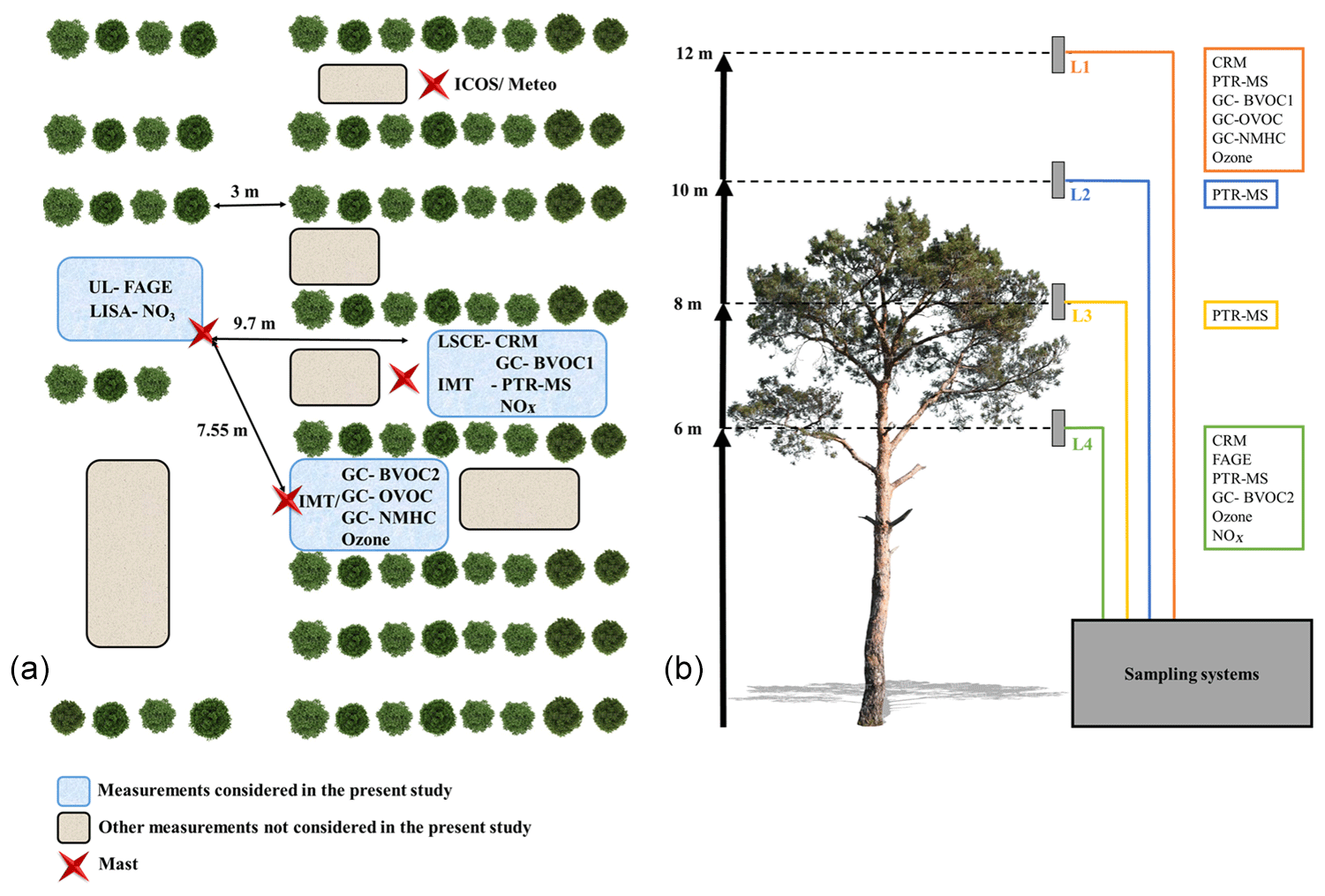
Figure 1Deployment of instruments at the measurement site. (a) The horizontal deployment and (b) the different sampling levels with respect to the average tree height.
Table 1Performance of the two OH reactivity instruments deployed during the LANDEX campaign.
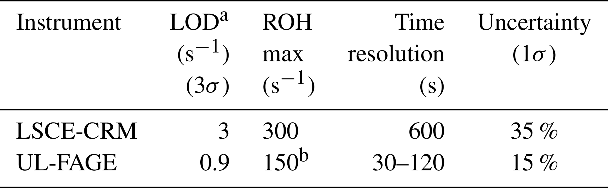
a LOD: limit of detection; b without dilution.
2.2.1 The comparative reactivity method (CRM) and instrument performance
The total OH reactivity was measured during the whole campaign, inside and above the canopy, by the LSCE-CRM instrument. This technique, first described by Sinha et al. (2008), is based on measuring the concentration of a reagent compound (pyrrole) that reacts with OH under different operating conditions (i.e., steps) at the output of the sampling reactor by a PTR-MS instrument. The first step consists of introducing pyrrole with dry nitrogen and dry zero air to measure the C1 level, which corresponds to the pyrrole concentration in the absence of OH. C1 accounts for potential photolysis due to photons emitted by the mercury lamp used to produce OH. During the second step, dry nitrogen and zero air are replaced by humid gases, and a pyrrole concentration C2 is measured. C2 is lower than C1 because pyrrole reacts with OH. In the last step, zero air is replaced by ambient air, which leads to competition between the reactions of OH with pyrrole and ambient trace gases. A C3 concentration higher than C2 is measured. The difference between C3 and C2 depends on the amount and reactivity of reactive species present in ambient air and is used to determine the total OH reactivity from Eq. (2), where it is assumed that pyrrole reacts with OH following pseudo-first-order reaction kinetics, i.e., [pyrrole] > [OH]:
where kp is the reaction rate constant of pyrrole with OH ( cm3 molecule−1 s−1; Atkinson, 1985).
This technique requires multiple corrections to derive reliable measurements of total OH reactivity due to (1) potential differences in relative humidity between C2 and C3, leading to different OH levels, (2) the spurious formation of OH in the sampling reactor when hydroperoxy radicals (HO2) react with nitrogen monoxide (NO), (3) not operating the instrument under pseudo-first-order conditions, and (4) the dilution of ambient air inside the reactor by the addition of N2 and pyrrole (Sinha et al., 2008; Michoud et al., 2015). In some CRM systems, corrections for potential NO2 and/or O3 artifacts are also considered (Michoud et al., 2015; Praplan et al., 2017). On one hand, NO2 is subject to photolysis leading to NO, which can subsequently react with HO2, yielding OH. On the other hand, O3 can also be photolyzed in the reactor, producing O(1D), which reacts further with H2O, yielding two OH radicals.
Intensive laboratory experiments and tests during the LANDEX field campaign were performed to characterize these corrections and assess the performances of the instrument over time. During the LANDEX field campaign, a slightly modified version of the CRM-LSCE instrument was used compared to the instrument previously deployed during the intercomparison experiment in the SAPHIR chamber (Fuchs et al., 2017). Indeed, this last study showed that the OH reactivity measured by all CRM instruments was significantly lower than the reactivity measured by the other instruments in the presence of monoterpenes and sesquiterpenes. A potential reason discussed for this discrepancy was the loss of terpenes in the inlet of the CRM instruments. The LSCE-CRM sampling system was built with o.d. non-heated perfluoroalkoxy (PFA) tubing and relied on a Teflon pump to introduce the sample into the reactor. In order to measure the total OH reactivity in a monoterpene-rich environment, several technical improvements were made on the previous version of the instrument described by Zannoni (2015). First, all the PFA sampling lines were replaced by o.d. sulfinert lines, continuously heated to around 50 ∘C to prevent condensation and minimize sorption processes. Second, temperature sensors were placed at several locations inside the system to monitor potential variations; the dew point was measured in the outflow through the pump to monitor humidity fluctuations, and the pressure was also monitored to make sure that measurements were performed at atmospheric pressure. All the flows going in and out of the reactor, the temperature at various places, the humidity, and the pressure in the reactor were recorded continuously to track potential variations.
Ambient air sampling
Ambient air was sampled through two o.d. sulfinert lines collocated on a mast close to the trailer (see Fig. 1a). The lines lengths were 8 m for the measurements performed inside the canopy and 12 m for those performed above. These lines were heated up to 50 ∘C as it was shown that losses of highly reactive molecules (i.e., β-caryophyllene) were negligible for temperatures above 20 ∘C (Kim et al., 2009).
During sampling, the airflow was driven through one line by two pumps. The first one was a Teflon pump located upstream of the reactor and the other one was that from the gas calibration unit (GCU) used to generate humid zero air from ambient air. Together, the two pumps allowed for air sampling between 1 and 1.2 L min−1, with the excess going to an exhaust.
CRM-LSCE system characterization
Several tests were performed before, during and after the campaign to assess the performance of the instrument operated during the whole campaign. The PTR-MS was calibrated at the beginning and at the end of the field campaign, showing good stability under dry and wet conditions (slope of 15.5±0.9 (1σ)). Regular C1 measurements were made to check the stability of the initial pyrrole concentration all along the campaign. C1 was 70.7±4.0 (1σ) ppbv.
Small differences in humidity observed between C2 and C3 were considered while processing the raw data. In order to assess this correction, experiments were performed to assess the variability of C2 on humidity by contrasting the change in C2 (ΔC2) for various changes in the ratio of m∕z 37 to m∕z 19 (Δ (m∕z 37-to-m∕z 19 ratios)), with m∕z 37 and m∕z 19 being representative of H3O+(H2O) and H3O+, respectively, and their ratio being proportional to humidity. During this campaign, three humidity tests were performed by varying the humidity in ambient air samples. These tests were in good agreement and showed a linear relationship between ΔC2 (ppbv) and Δ (m∕z 37-to-m∕z 19 ratio) with a slope of −89.18. The correction was applied as discussed in Michoud et al. (2015).
An important assumption to derive ROH from Eq. (2) is to operate the instrument under pseudo-first-order conditions (i.e., [pyrrole] ≫ [OH]), which is not the case with current CRM instruments. To determine the correction factor for the deviation from pseudo-first-order kinetics, injections of known concentrations of isoprene ( cm3 molecule−1 s−1, 1–120 ppbv) and α-pinene ( cm3 molecule−1 s−1, 3–190 ppbv) (Atkinson, 1985) were performed before and after the field campaign since they represent the dominant species in this forest ecosystem.
The measured OH reactivity obtained from these tests was then compared to the expected OH reactivity, leading to a correction factor that is dependent on the pyrrole-to-OH ratio. Therefore, standard OH reactivity experiments were conducted at different pyrrole-to-OH ratios ranging from 1.7 to 4.0, which encompass the ratio observed most of the time during the campaign. These tests led to a correction factor .
NO mixing ratios were lower than 0.5 ppbv (corresponding to the detection limit of the NOx monitor deployed during LANDEX) most of the time for the measurement time periods used in this study, and no correction was applied for the spurious formation of OH from the HO2 + NO reaction. Similarly, for NO2, no correction was applied due to the low ambient mixing ratio of 1.1±0.8 ppbv. Regarding O3, no dependency was seen for LSCE-CRM based on previous experiments (Fuchs et al., 2017). Therefore, no correction was applied. The correction (D) on the reactivity values due to the dilution was around 1.46 during the campaign. Thus, the total OH reactivity may be expressed as
Finally, overall uncertainties were estimated at 35 % (1σ) for the measured OH reactivity by the CRM (Zannoni, 2015).
Table 2 reports a summary of the corrections resulting from our tests and their impact on measurements. As shown in Table 2, the application of (F) for the deviation from pseudo-first-order kinetics induces the largest correction, with an absolute increase of 10.4 s−1 on average. Furthermore, this factor (F) has the largest relative uncertainty, with ±36 % against ±2 % for the humidity correction factor.
Table 2Summary of corrections applied to raw reactivity data for LSCE-CRM. Correction coefficients are obtained from experiments performed before, during and after the field campaign.

2.2.2 UL-FAGE reactivity instrument
Total OH reactivity was measured at a different location inside the canopy from 13 to 19 July using the LP-LIF instrument of the PC2A laboratory (UL-FAGE reactivity), which has already been used in several intercomparisons and field campaigns (Hansen et al., 2015; Fuchs et al., 2017). The reactivity instrument comprises three parts: the photolysis laser, the photolysis cell (reaction tube) and the LIF cell based on the FAGE technique. The photolysis laser is used to generate OH radicals within the photolysis cell by the photolysis of O3 in the presence of water vapor. The photolysis laser is a YAG laser (Brilliant EaZy, QUANTEL) with a doubling and a quadrupling stage providing radiation at 266 nm with a repetition rate of 1 Hz. The photolysis beam is aligned at the center of the photolysis cell and is expanded (diameter of 4 cm reaching the entrance of the cell) by two lenses (a concave one mm and a convex with f=150 mm) in order to increase the photolysis volume and to limit the diffusion effect in the photolysis cell.
This photolysis cell is a stainless-steel cylinder with an internal diameter of 5 cm and a length of 48 cm. It presents two openings on opposite sides, one as an entrance for the air samples and the second connected to a pressure monitor (Keller PAA-41) to measure the pressure inside the cell. Ambient or humid clean air (which is produced by passing a fraction of dry synthetic air with a purity of 99.8 % through a water bubbler, called zero air, used to determine the OH reactivity in the absence of reacting species) is injected through the first opening with a small flow of synthetic air (about 20 mL min−1) passing through an ozone generator (Scientech) to generate an ozone concentration of about 50 ppbv in the total flow. The ozone concentration is chosen to produce enough OH to have a good signal-to-noise ratio but kept low enough to minimize reactions involving O3.
The sampled mixture is continuously pumped into the FAGE cell (pressure 2.3 Torr) by a dry pump (Edwards, GX 600L), and the LIF signal is collected by a channel photomultiplier (CPM; Perkin Elmer MP1982), an acquisition card and a LabView program. The detection of the fluorescence is synchronized with the photolysis laser pulses by delay generators. The OH reactivity time resolution was at the minimum set to be 30 s, meaning that each OH decay was accumulated over 30 photolysis laser shots and fitted by a mono-exponential decay. The number of sets of 30 photolysis laser shots accumulated is determined according to the signal-to-noise ratio (SNR) obtained (typically 4). When the SNR is lower, a set of 30 OH decays is added to the previous one and so on until reaching the criteria. As the reactivity and the humidity vary along the day, SNR varies as a function of the ambient species concentrations. In order to check the consistency of the OH reactivity measurements, the well-known (CO + OH) reaction rate constant was measured. Different CO concentrations, from 4×10¹³ to 3.7×1014 cm−3 in humid zero air, are injected in the photolysis cell, allowing us to measure reactivities ranging from 10 to 90 s−1 and to determine (using a linear regression: R2=0.97) a rate constant of cm3 molecule−1 s−1, in good agreement with the reference value of cm3 molecule−1 s−1 (Atkinson et al., 2006) at room temperature. Under these conditions (absence of NO), HO2 formed by the reaction of CO + OH is not recycled in OH and does not interfere with the measurements of OH.
Ambient air sampling
Ambient air was sampled in the canopy at about 5 m through a PFA line (diameter 1∕2 in.), with a PFA filter being installed at the entrance of the tube to minimize particle or dust sampling. In the photolysis cell, the gas flow was sampled at 7.5 L min−1 and the pressure was approximately 740 Torr, i.e., lower than the atmospheric pressure due to the restriction of the flow through the Teflon sampling line. For the reactivity measurements in zero air, synthetic air from a cylinder was used and a part of the flow (2 L min−1) passed through a bubbler filled with Milli-Q water to reach a water vapor concentration of about 3000 ppmv.
ROH,zero analysis
In order to determine the OH reactivity in ambient air, ROH,ambient, it is necessary to subtract the reactivity measured using zero air, ROH,zero, which represents OH losses not related to gas-phase reactions with the species of interest that are present in the ambient air but rather those due to wall losses or diffusion to the reactivity measured.
Zero air tests were conducted twice a day (in the morning and at night) when the reactivity measurements took place. The average of all experiments performed with zero air leads to a mean value of s−1. This value was therefore chosen as kzero for the whole campaign.
2.3 Ancillary measurements and corresponding locations
Measurements of VOCs (Table 3) were performed at different locations (Fig. 1) by a proton transfer reaction mass spectrometer (PTR-MS) and four online gas chromatographic (GC) instruments. Ozone scrubbers (copper tube impregnated with KI) and particle filters were added to the inlets of all GC sampling lines. Losses of BVOCs in these ozone scrubbers were investigated under similar sampling conditions in the absence and presence of O3 (Mermet et al., 2019). The scrubbers exhibited less than 5 % losses for most non-oxygenated BVOCs, whereas in the presence of ozone, losses were relatively higher for some BVOCs but remained lower than 15 % (lower than 5 % for α- and β-pinene). High flow rates were applied in the sampling lines: 1 L min−1 for GC instruments and 10 L min−1 for the PTR-MS; therefore, the contact time between ambient BVOCs and the particle filters was extremely short and no significant losses are expected.
GC-BVOC1 is a gas chromatograph coupled to a flame ionization detector (airmoVOC C6–C12, Chromatotec) used by LSCE to monitor high-carbon VOCs (C6–C12) at 12 m of height with a time resolution of 30 min. Sampling was undertaken for 10 min. The instrument sampled ambient air with a flow rate of 60 mL min−1. Once injected, the sample passed through a capture tube containing the adsorbent Carbotrap C for VOC preconcentration at room temperature; the capture tube is then heated up to 380 ∘C and the sample is introduced into the separating column (MXT30CE; i.d. 0.28 mm, length 30 m, film thickness 1 µm), with hydrogen as the carrier gas. During the campaign, calibrations were performed with a certified standard containing a mixture of 16 VOCs (including eight terpenes) at a concentration level of 2 ppbv (National Physical Laboratory, Teddington, Middlesex, UK). Three calibrations were performed three times (at the beginning, in the middle and at the end of the campaign). As they were showing reproducible results (within 5 % for all the terpenes except cineole), a mean response factor per VOC was used to calibrate the measurements. Note that limonene and cymene had close retention times, which led to overlapping peaks, and for this reason only the sum of both compounds has been reported. For further details, refer to Gros et al. (2011). The sampling was done using a 13 m long sulfinert heated line () connected to an external pump for continuous flushing.
GC-BVOC2 is an online thermodesorber system (Markes UNITY 1) coupled to a GC-FID (Agilent). It was used to monitor 20 C5–C15 BVOCs, including isoprene, α- and β-pinene, carenes, and β-caryophyllene at the 6 m height with a time resolution of 90 min. Ambient air was sampled at a flow rate of 20 mL min−1 for 60 min through a sorbent trap (Carbotrap B) held at 20 ∘C by a Peltier cooling system. The sample was thermally desorbed at 325 ∘C and injected into BPX5 columns (60 m × 0.25 mm × 1 µm) using helium as a carrier gas (30 min). Calibrations were performed at the beginning, in the middle and at the end of the campaign with a certified standard mixture (National Physical Laboratory – NPL; Teddington, Middlesex, UK, 2014) containing 33 VOCs (including four BVOCs: α-pinene, β-pinene, limonene and isoprene) at a concentration of 4 ppbv each. The sampling was done using a 10 m long sulfinert line () heated at 55 ∘C and connected to an external pump to adjust the sampling flow rate at 1 L min−1. The method has been optimized in terms of temperature of the thermodesorption, the column, the sampling volume and sampling line including a scrubber. Tests showed a low response for some compounds (i.e., sabinene, terpinolene, etc.); however, the most abundant compounds were well measured. More details about the optimization and the tests performed can be found in Mermet et al. (2019).
GC-NMHC is an online GC equipped with two columns and a dual FID system (Perkin Elmer®) that was described in detail elsewhere (Badol et al., 2004). It was used to monitor 65 C2–C14 non-methane hydrocarbons (NMHCs), including alkanes, alkenes, alkynes and aromatics, at the 12 m height with a time resolution of 90 min. Ambient air was sampled at a flow of 15 mL min−1 for 40 min through a Nafion membrane and through a sorbent trap (Carbotrap B and Carbosieve III) held at −30 ∘C by a Peltier cooling system. The trap was thermodesorbed at 300 ∘C and the sample was introduced in the GC system. The chromatographic separation was performed using two capillary columns with a switching facility. The first column, used to separate C6–C14 compounds, was a CP-Sil 5 CB (50 m × 0.25 mm × 1 µm), while the second column for C2–C5 compounds was a plot Al2O3∕Na2SO4 (50 m × 0.32 mm × 5 µm). Helium was used as a carrier gas. Calibrations were performed at the beginning, middle and end of the campaign with a certified standard mixture (NPL; Teddington, Middlesex, UK, 2016) containing 30 VOCs at a concentration level of 4 ppbv each. The sampling was done using a 13 m long sulfinert line () heated at 55 ∘C and connected to an external pump for continuous flushing at 2 L min−1.
GC-OVOC is an online GC-FID (Perkin Elmer®) used to monitor 16 C3–C7 oxygenated VOCs (OVOCs), including aldehydes, ketones, alcohols, ethers, esters and six NMHCs (BVOCs and aromatics). A detailed description can be found in Roukos et al. (2009). The measurements were performed at the 12 m height with a time resolution of 90 min. Ambient air was sampled at a flow rate of 15 mL min−1 for 40 min through a water trap (cold finger, −30 ∘C) and a quartz tube filled with Carbopack B and Carbopack X held at 12.5 ∘C. VOCs were thermally desorbed at 280 ∘C and injected into CP-Lowox columns (30 m × 0.53 mm × 10 µm) using helium as a carrier gas. Calibrations were performed three times during the campaign using a standard mixture (Apel Riemer, 2016) containing 15 compounds. This mixture was diluted with humidified zero air (RH = 50 %) to reach VOC levels of 3–4 ppbv. The sampling was done with the same sampling system as the GC-NMHC. The sulfinert material chosen for all GC sampling lines and used in the LSCE-CRM sampling system is recommended by ACTRIS (2014). High flows were set in the lines (residence time of less than 8 s) that were heated up to 50 ∘C to minimize the losses of potential reactive species. Filters and scrubbers were changed twice for the GC-BVOC1 and one time for the other GC instruments.
The PTR-MS (PTR-QiToFMS, IONICON Analytic GmbH) sequentially measured trace gases at four levels (L1 = 12 m, L2 = 10 m, L3 = 8 m, L4 = 6 m) with a cycle of 30 min (6 min at each level and 6 min of zero air). The drift tube was operated at a pressure of 3.8 mbar, a temperature of 70 ∘C and an E∕N ratio of 131 Td. Four identical sampling lines of 15 m were used to sample ambient air at each height. The lines (PFA, o.d.) were heated at 50 ∘C and were constantly flushed at 10 L min−1 using an additional pump and rotameters. Indeed, Kim et al. (2009) tested losses of β-caryophyllene in similar operating conditions. The authors varied the temperature from zero to 40 ∘C, showing that losses of β-caryophyllene are negligible above 20 ∘C. The residence time was lower than 2 s.
Teflon filters were used to filter particles at the entrance of the sampling lines. The PTR-MS drew ambient air at a flow rate of 300 mL min−1 from the different lines using Teflon solenoid valves and a 1.5 m long inlet (PEEK, o.d.) heated at 60 ∘C. Zero air was generated using a gas calibration unit (GCU; IONICON Analytic GmbH) containing a catalytic oven and connected to L1. Ion transmissions were calibrated over the 21–147 Da mass range every 3 d using the GCU and a certified calibration mixture provided by IONICON (15 compounds at approximately 1 ppmv, including methanol, acetaldehyde, acetone, aromatic compounds and chlorobenzenes). Measurements of methanol, acetonitrile, acetaldehyde, acetone, isoprene, methacrolein + methylvinylketone + fragment ISOPOOH, methylethylketone, the sum of monoterpenes, the sum of sesquiterpenes, acetic acid, nopinone and pinonaldehyde, obtained from levels 1 and 4 corresponding to the levels at which OH reactivity measurements were performed, are discussed in this article. Sesquiterpenes, acetic acid, nopinone and pinonaldehyde measurements were not corrected for fragmentation in the drift tube, and we cannot rule out the detection of other isomers at these masses such as glycolaldehyde for acetic acid measurements.
Inorganic traces gases (O3 and NOx) were measured by commercial analyzers deployed by IMT-Lille-Douai (L1 to L4 for O3) and EPOC (L4 for NOx). The nitrate radical (NO3) was measured using an IBB-CEAS instrument (incoherent broadband cavity absorption spectroscopy) developed by the LISA (Laboratoire Interdisciplinaire des Systèmes Atmosphériques) research group and deployed for the first time on site during the LANDEX field campaign. Meteorological parameters such as temperature, relative humidity, global radiation, vertical turbulence, wind speed and wind direction were monitored using sensors already available at the ICOS measurement site. More details can be found in Kammer et al. (2018).
Table 3Summary of supporting measurements performed inside and/or above the canopy.
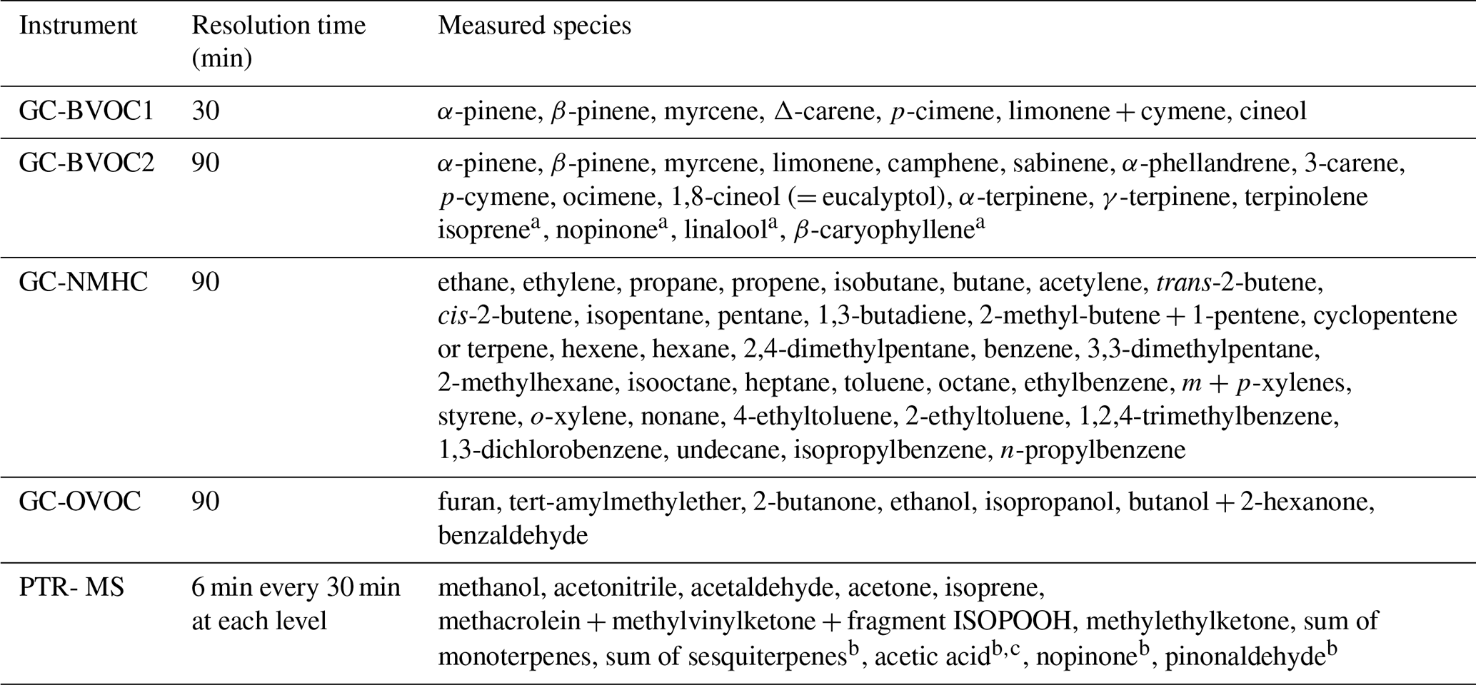
a These compounds were not considered in the calculation of the weighted k rate constant for the reaction of monoterpenes with OH. Nopinone, linalool and β-caryophyllene had relatively low contributions to OH reactivity that were around 0.02, 0.37 and 0.18 s−1 on average, respectively. Maximum contributions did not exceed 2.2 s−1 for linalool and 1.5 s−1 for β-caryophyllene. b Fragmentation was not corrected for, and reported concentrations are likely lower limits. c Potential interferences from isomeric compounds such as glycolaldehyde.
2.4 OH reactivity calculation
As different instruments were available to quantify VOCs at different locations (Fig. 1 and Table 3), a selection of the data used to calculate the OH reactivity (Eq. 1) was made based on data availability for the different instruments (Table S1 in the Supplement). Since measurements from the PTR-MS instrument cover the whole campaign and were performed at the same heights as OH reactivity measurements, these measurements, including methanol, acetonitrile, acetaldehyde, acetone, isoprene, methacrolein + methylvinylketone + fragment ISOPOOH, methylethylketone and the sum of monoterpenes, were selected to calculate the OH reactivity and to evaluate the potential missing OH reactivity at both levels. However, using only this set of data presents some limitations.
-
The PTR-MS only measures the sum of monoterpenes (m∕z 137), while the detected monoterpenes are speciated by the GCs.
-
It was observed that isoprene measurements at m∕z 69 were disturbed by the fragmentation of some terpenic species (Kari et al., 2018; Tani, 2013), which led to a significant impact on the nighttime measurements when isoprene was low.
-
Some NMHCs and OVOCs measured by GC at the 12 m height were not measured by the PTR-MS. This requires an assessment of the contribution of these additional species to the total OH reactivity for both heights.
To overcome these limitations, several tests were made to evaluate the reliability of the PTR-MS data to calculate the OH reactivity.
-
In order to use the sum of monoterpenes measured by the PTR-MS to calculate the total OH reactivity, it was necessary to determine a weighted rate constant for the reaction of monoterpenes with OH. After checking the consistency between the two GCs (BVOC1 and BVOC2; see Sect. S2) and comparing the sum of monoterpenes measured by each GC to the PTR-MS measurements (simultaneous measurements at the same height; Fig. S2b and c), the weighted rate constant was calculated as the sum of the rate constants of each OH + monoterpene reaction multiplied by the average contribution of each specific monoterpene to the sum. The contribution of each monoterpene was calculated by dividing the concentration of the eight speciated monoterpenes that were measured by both GCs (α-pinene, β-pinene, myrcene, Δ-carene, p-cimene, limonene + cymene, cineol) by their total concentration (Fig. S3a). The weighted rate constant is defined as
where Fi represents the contribution of each individual species to the total concentration of monoterpenes, and is the corresponding rate constant with OH. The reaction rate constant of the different trace species quantified in the field were taken from the literature (Atkinson et al., 2006). The OH reactivity of monoterpenes measured by PTR-MS was calculated according to the following equation:
where [MT] represents the sum of monoterpenes measured by PTR-MS.
The calculated OH reactivity inside and above the canopy (Fig. S3b and e) from (i) the use of the weighted OH reaction rate constant and the total concentration of monoterpenes measured by GC and (ii) the use of individual species and their associated rate constants is in relatively good agreement as shown by the scatter plots. At a slope of 0.95, R2=0.99 has been obtained using the monoterpenes measured with the GC-BVOC1 at 12 m (Fig. S3c); at a slope of 0.94, R2=1.0 was obtained using the same eight compounds commonly monitored with GC-BVOC1 but measured at 6 m with GC-BVOC2 (Fig. S3f). When replacing the total concentration of monoterpenes measured by GCs by the PTR-MS measurements, slopes of 1.22 and 1.19 were obtained at 12 and 6 m heights, respectively (Fig. S3d and g). This increase in the slope values is likely due to an underestimation of the total monoterpene concentration by the GC instruments since these instruments only measured the most abundant monoterpenes present at the site. We cannot rule out a small overestimation of monoterpenes by the PTR-MS since fragments from other species such as sesquiterpenes could be detected at the monoterpene m∕z. However, this interference should be negligible due to the low concentration of ambient sesquiterpenes. These results are in agreement with the scatter plots comparing the sum of monoterpenes measured by GC and by PTR-MS (slopes of 1.29 and 1.10 at the 12 and 6 m heights, respectively; see Fig. S2b and c). Thus, the PTR-MS data were used to calculate the OH reactivity from monoterpenes for both heights, with a weighted reaction rate constant of cm3 molecule−1 s−1 at the 12 m height and cm3 molecule−1 s−1 at the 6 m height.
-
As mentioned above, some monoterpenes have been observed to fragment at m∕z 69.0704, which would result in an interference for isoprene measurements. In order to use the PTR-MS data for this species (the only instrument measuring isoprene at 12 m), the contribution of monoterpenes to m∕z 69 has been estimated by comparing the GC-BVOC2 and PTR-MS measurements of isoprene performed at 6 m. This comparison showed that approximately 4 % of the monoterpene concentration measured by PTR-MS had to be subtracted from that measured at m∕z 69.0704 to get a good agreement between the PTR-MS and GC-BVOC2 measurements of isoprene, as shown in Fig. S4a.
-
A large range of NMHCs and OVOCs was measured at the 12 m height only by GC-NMHC and GC-OVOC (Table 3). Butanol (from scanning mobility particle sizer – SMPS – exhausts) was also checked and found to be negligible at 12 m and highly and rapidly variable at 6 m (short peaks). NO and NO2 were only measured at the 6 m height. The mean NO mixing ratio was below the LOD for the measurement period, and NO2 was around 1.1±0.8 ppbv on average. Thus, it was chosen not to take these species into account in the OH reactivity calculations. However, sensitivity tests were performed in order to compute their relative contribution to OH reactivity (see Sect. 3.5 and Figs. S5 and S6). Regarding methane and carbon monoxide, an estimation was made given their relatively low k reaction rate coefficient with OH, resulting in mean concentration values of 2000 and 150 ppbv, respectively.
The above limitations are summarized in Table S7. The data used to calculate the OH reactivity have been resampled to 1 min based on a linear interpolation (see Table 3 for the respective time resolution of the different instruments). This time base was chosen to be comparable to the time resolution of the UL-FAGE reactivity instrument in order to keep the dynamics in OH reactivity variability.
Measurements performed by both instruments at the same location were first compared to evaluate the agreement between the two techniques. The horizontal variability of total OH reactivity (same height) is also discussed. A second part of the Results section is dedicated to a description of the total OH reactivity variability on the vertical scale with some meteorological parameters. A comparison between measured and calculated OH reactivity for both the 6 and 12 m heights as well as a description of the BVOC contributions to the measured OH reactivity are then presented. Finally, we discuss the missing OH reactivity observed during this campaign and its possible origin.
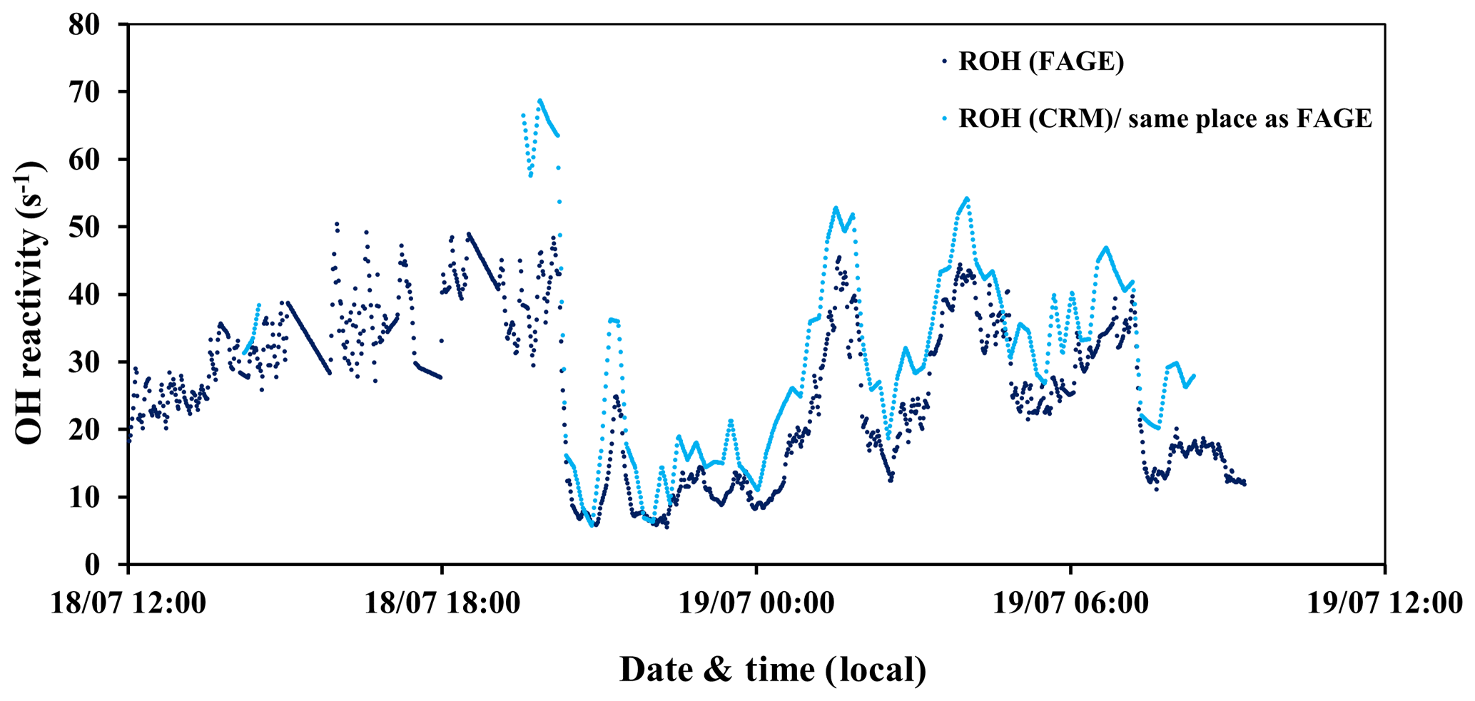
Figure 2Time series of total OH reactivity measured by the UL-FAGE (dark blue) and LSCE-CRM (light blue) instruments from 18 to 19 July 2017 at the same location inside the canopy.
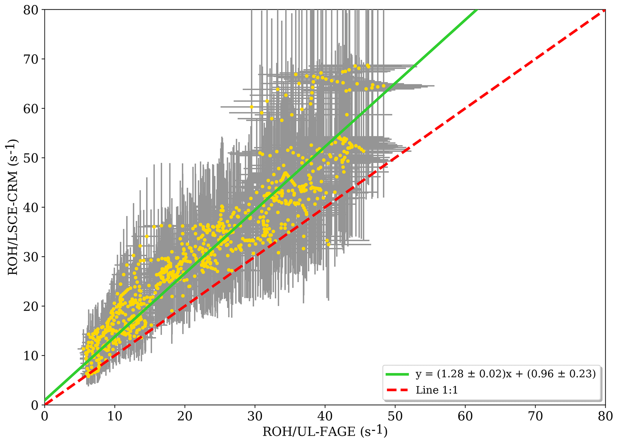
Figure 3Measured reactivity by the LSCE-CRM instrument as a function of the measured reactivity by UL-FAGE when both instruments were measuring at the same location within the canopy (data resampled with a time resolution of 1 min). Errors bars represent the overall systematic uncertainty (1σ) that is around 15 % and 35 % for LP-LIF and the CRM, respectively.
3.1 Comparison between LSCE-CRM and UL-FAGE measurements
3.1.1 Intercomparison of LSCE-CRM and UL-FAGE OH reactivity measurements at the same location
A direct comparison between the LSCE-CRM and UL-FAGE reactivity instruments was done during the last 2 d of the campaign (Fig. 2). The sampling line of LSCE-CRM was moved to be collocated with the sampling line of UL-FAGE. Both instruments were measuring at the same location inside the canopy level, above the UL container at 5 m of height. In this way the comparison between the two instruments was made possible while minimizing variabilities that could be related to the heterogeneity in ambient air. During this period, similar values were measured by both instruments, as shown in Fig. 2, with total OH reactivity ranging between 5 and 69 s−1. The lowest values were observed during daytime.
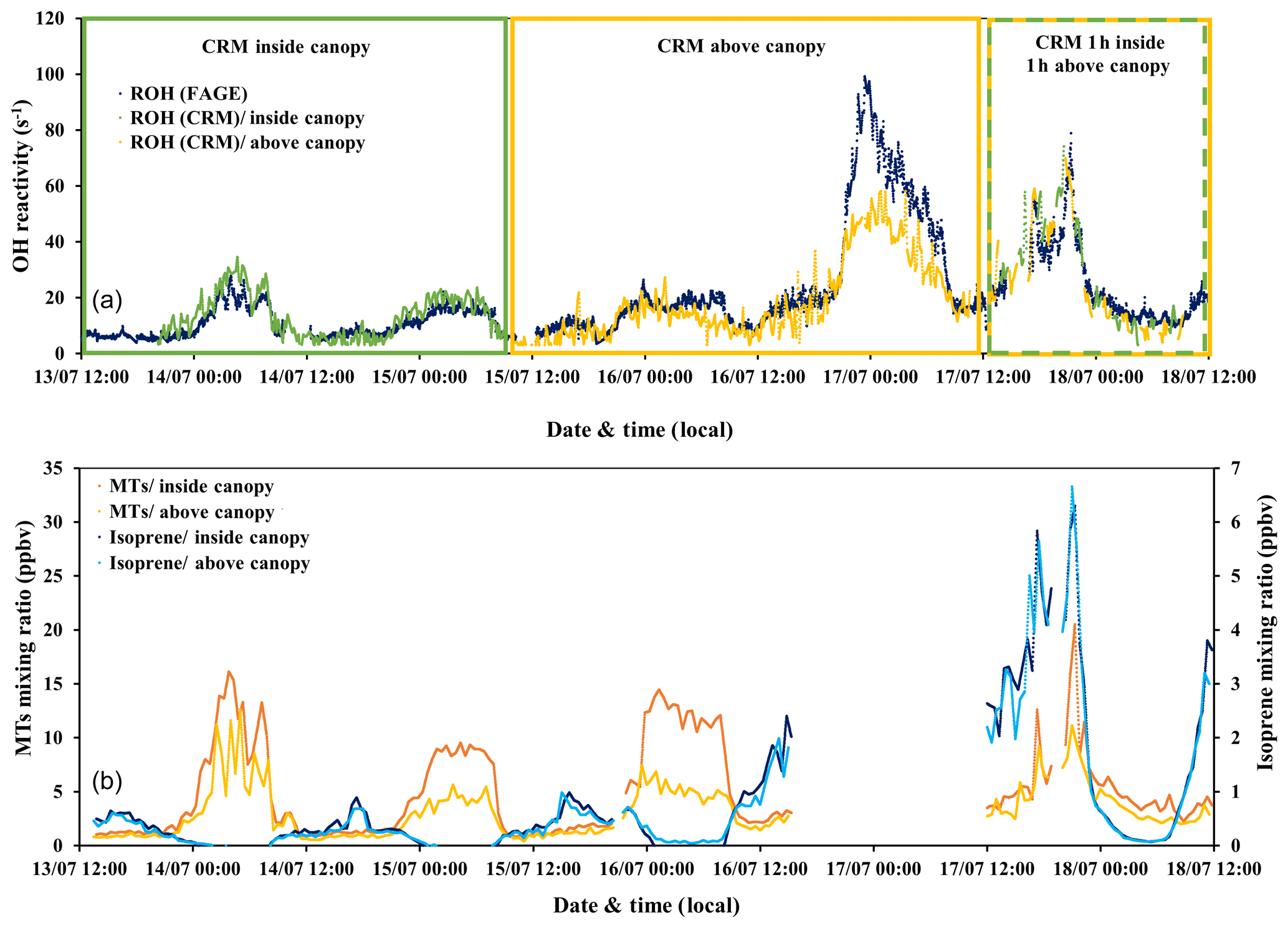
Figure 4(a) Time series of total OH reactivity measured by the UL-FAGE and LSCE-CRM instruments from 13 to 18 July 2017 (a). Dark blue symbols represent the measured reactivity by UL-FAGE; green and yellow symbols represent the measured reactivity by LSCE-CRM inside and above the canopy, respectively. (b) The sum of monoterpenes (MTs) and isoprene measured with the PTR-MS in the field for the same period. Dark blue and light blue dots correspond to isoprene concentrations at 6 and 12 m of height, respectively. Orange and yellow dots represent monoterpene concentrations at 6 and 12 m of height, respectively.
When OH reactivity measurements from LSCE-CRM are plotted versus OH reactivity measurements from UL- FAGE (Fig. 3), the linear regression exhibits an R2 of 0.87. Applying the orthogonal distance regression technique, which takes into account the uncertainties on LSCE-CRM and UL-FAGE measurements, a slope of 1.28±0.02 and an intercept of 0.96±0.23 s−1 are obtained. These results indicate that both instruments respond similarly (within 30 %) to changes in OH reactivity with a relatively low intercept. This intercept can be due to an overestimation of LSCE-CRM measurements, an underestimation of the UL-FAGE measurements or both. Nevertheless, it stays within the range of uncertainties. It is worth noting that the higher points of OH reactivity observed in Fig. 3 correspond to the period from 19:30 to 20:00 LT (local time) on 18 July when the ambient relative humidity increased quickly by 20 %, which was not seen on previous days and may have interfered with LSCE-CRM OH reactivity measurements.
3.1.2 LSCE-CRM and UL-FAGE OH reactivity measurements at two different locations inside the canopy
From 13 to 15 July midday (first period) and from 17 to 18 July midday (second period), the two instruments were sampling at the same height but from different horizontal locations within the canopy (with sequential within- and above-canopy measurements for CRM during the second period). The horizontal distance between the two inlets was around 10 m as shown in Fig. 1. Similar trends in OH reactivity are seen between the two datasets, even if the first period was associated with a clear vertical stratification (Fig. 4, green frame), leading to higher concentrations of monoterpenes within the canopy, whereas the second period was characterized by a higher vertical mixing (mean m s−1) leading to similar concentrations of monoterpenes at the two heights (Fig. 4, dashed green–yellow frame). These observations are linked to the vertical turbulence that influences BVOC levels inside and above the canopy, resulting in a more or less important vertical stratification, as discussed in Sect. 3.2.
At the same height but different horizontal locations, the linear regression of LSCE-CRM data plotted against UL-FAGE data (not shown) indicates a good correlation with an R2 of 0.87. Using the orthogonal distance regression technique, both datasets show a good agreement with a slope of 1.28±0.02 and an intercept of (first and second period). Compared to the results at the same location (vertical and horizontal), the slopes and the correlation coefficients are the same. Only the intercept differs slightly ( compared to 0.96±0.23). This change could be related to air mass inhomogeneities, which could be systematically less reactive at one location compared to the other one. From these observations, we can conclude that reactivity measurements performed at different horizontal locations are consistent and that inhomogeneities in ambient air can lead to differences on the order of several seconds.
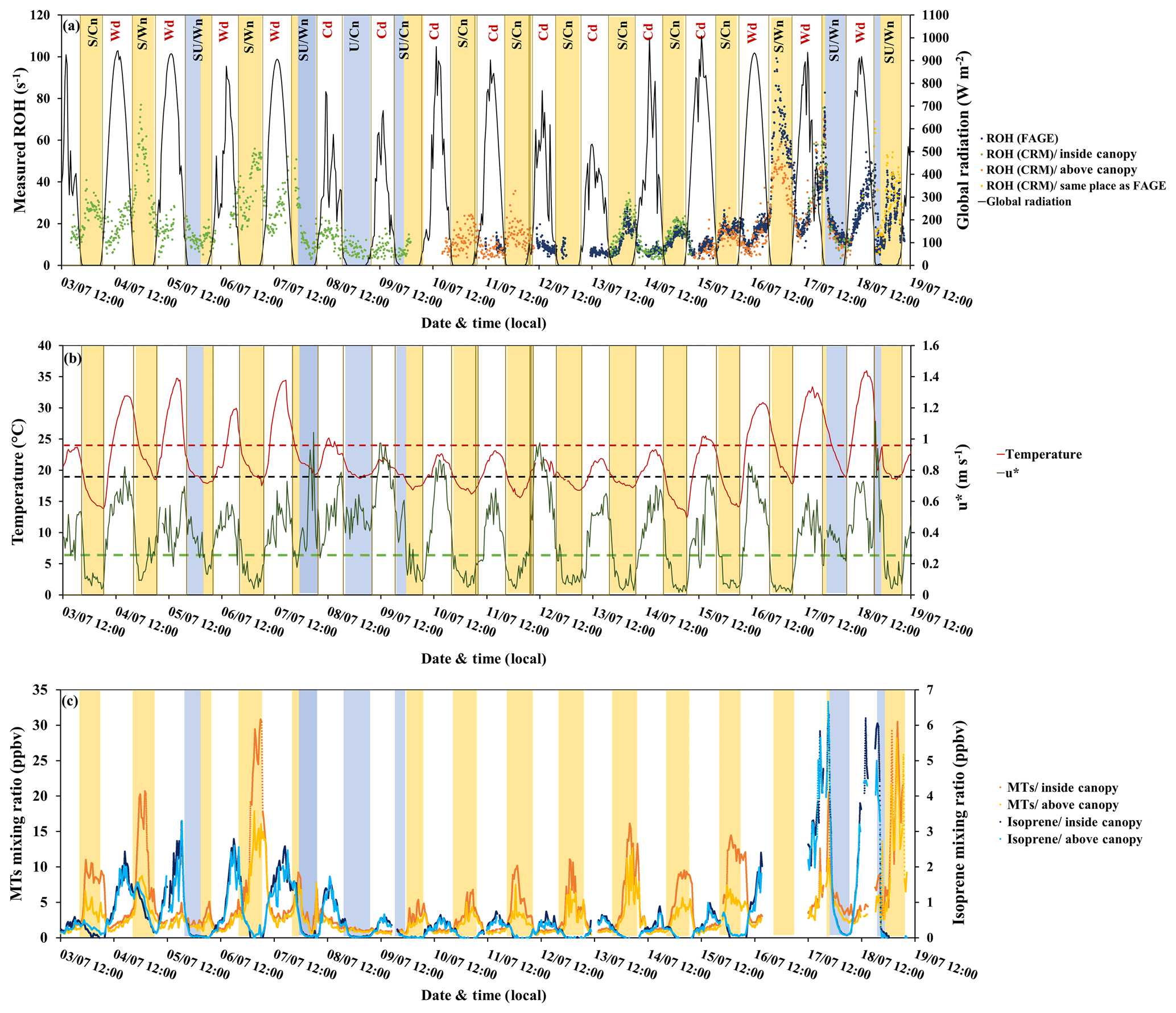
Figure 5Variability of measured OH reactivity by LSCE-CRM and UL-FAGE inside and above the canopy with (a) global radiation (black), (b) temperature (red), friction velocity (green), and (c) monoterpene and isoprene concentrations. Yellow stripes indicate stable nighttime atmospheric conditions (S nights with mean m s−1), and blue stripes indicate unstable nighttime conditions (U nights with mean m s−1). Class SU includes nights with stable and unstable atmospheric conditions (blue + yellow stripes). Wn and Wd stand for warm nights and warm days, respectively. Cn and Cd stand for cooler nights and cooler days, respectively. Red dashes and black dashes indicate the temperature thresholds to distinguish warm and cool days and nights, respectively. Green dashes indicate the friction velocity threshold to distinguish stable and unstable nights.
3.2 Measured OH reactivity and meteorological parameters
Figure 5a and b shows the variability of total OH reactivity measured inside and above the canopy by LSCE-CRM and UL-FAGE, together with global radiation, temperature and friction velocity. Considering the whole campaign, the measured OH reactivity at both heights shows a diurnal trend ranging between LOD (3 s−1) and 99 s−1 inside canopy and between LOD and 70 s−1 above the canopy, with maximum values of OH reactivity mostly recorded during nights. These OH reactivity levels are larger than other measurements performed in forested environments (Yang et al., 2016; Dusanter and Stevens, 2017), with maximum values of approximately 80 s−1 reported for a tropical forest (Edwards et al., 2013).
The predominant meteorological parameter that had a role in OH reactivity levels was friction velocity. It traduces the vertical turbulence intensity that was high during the day (mean daytime m s−1) and lower during most nights (mean nighttime m s−1). Based on this parameter, nighttime OH reactivity (between 21:00 and 06:00 LT of the next day) was separated into three classes:
-
class S involves stable atmospheric conditions (mean m s−1),
-
class U involves unstable atmospheric conditions (mean m s−1), and
-
class SU involves stable and unstable conditions during the same night.
The lower vertical turbulence intensity, observed for S nights as well as for some hours of SU nights, led to a lower boundary layer (Saraiva and Krusche, 2013) and a significant nocturnal stratification within the canopy, with higher concentrations of primary compounds within the canopy (Fig. 5c). These stable atmospheric conditions, together with no photochemical oxidation of BVOCs, resulted in higher total OH reactivity during these nights due to higher BVOC concentration even though the emissions are lower compared to daytime (Simon et al., 1994).
Another important parameter to consider is ambient temperature, which is known to enhance BVOC emissions during the day when stomata are open and which also plays a role for nighttime emissions due to permeation, even though stomata are closed in the dark (Simon et al., 1994). Considering temperature, two subclasses can be added to nighttime OH reactivity classification: the subclass Wn corresponding to warm nights (nights with mean T≥18.9 ∘C, which is the mean nighttime temperature over the whole campaign) and the subclass Cn that includes cooler nights (nights with mean T<18.9 ∘C). Thus, comparing S/Wn nights and S/Cn nights, it can be seen that, for similar turbulent conditions, the magnitude of the measured OH reactivity was temperature dependent. Indeed, higher OH reactivity values were linked to higher ambient temperatures: the nights of 4–5, 6–7 and 16–17 July (S/Wn) were characterized by an average temperature of 21 ∘C compared to 16.6 ∘C for the nights with lower OH reactivity (S/Cn).
Regarding the period when measurements were done simultaneously at both heights (15 to 18 July, LSCE-CRM above the canopy and UL-FAGE within the canopy), we can analyze the effect of turbulence on the above- and within-canopy differences. For the night of 16–17 July (S/Wn) when the vertical turbulence was relatively low, total OH reactivity measured above the canopy (LSCE-CRM) was lower than the one measured inside the canopy by a mean factor of 1.6 (UL-FAGE reactivity) despite similar general trends. For the night of 17–18 July (SU/Wn), stable atmospheric conditions started to settle at the beginning of the night (20:30 LT), inducing a similar stratification to that observed on the previous nights. However, this situation did not last the whole night since these stable conditions were disturbed by higher turbulences around 21:00 LT. This led to a decrease in OH reactivity values going to similar levels inside and above the canopy. A similar event occurred during the night of 18–19 July, when three OH reactivity peaks showed up that were not correlated with the variation of turbulence intensity or with temperature changes. However, it is worth noting that during this night, intense wind, rain and thunder occurred, which could have led to the observed bursts of BVOCs (Nakashima et al., 2013), leading to distinct peaks of BVOCs and total OH reactivity and thus relatively high total OH reactivity compared to other nights from the same class.
Total OH reactivity also increased during the day, although to a lesser extent than during nighttime, and reached a daytime maximum of up to 74.2 s−1 inside the canopy and 69.9 s−1 above the canopy, following the same trends as temperature and solar radiation. Temperature appeared to be an important driving factor of total OH reactivity during daytime hours; therefore, daytime OH reactivity was divided into two classes: class Wd with warm conditions (mean daytime T≥24 ∘C) and class Cd with cooler temperatures (mean daytime T<24 ∘C), as indicated in Fig. 5. The solar radiation also played a role in daytime OH reactivity since it is responsible for initiating the emission of some compounds like isoprene that are light and temperature dependent. Thus, with the first rays of sunlight, the emission and the concentration of isoprene increased, leading to an increase in total OH reactivity.
Examining BVOC profiles (Fig. 5c), we can see how the variability of primary BVOC concentrations can explain the day–night variability of total OH reactivity. Indeed, monoterpenes, which are the main emitted compounds in this ecosystem, were influenced by vertical turbulence and nighttime temperature, exhibiting a diurnal profile with maxima during stable nights and minima during daytime. Under stable atmospheric conditions (class S), monoterpene concentrations started to increase at the beginning of the night (between 20:00 and 21:00 LT), corresponding to the time of day when the turbulence intensity started to drop and the nocturnal boundary layer started to build up. Maximum mixing ratios were reached in the middle of the night, corresponding to a lower dilution in the atmosphere and a lower oxidation rate (low OH concentrations, nitrate radical mixing ratios lower than the LOD of 3 ppt min−1 most of the time and BVOC chemistry with ozone generally slower than during daytime; Fuentes et al., 2002). Finally, the monoterpene concentration dropped as soon as the first sunlight radiation broke the stable nocturnal boundary layer, inducing lower levels of OH reactivity. Under these conditions, the concentration of monoterpenes inside the canopy was higher than above the canopy, showing a clear stratification consistent with the differences seen in total OH reactivity at the different heights. In contrast, during turbulent night hours (class U and SU), the concentration of monoterpenes was lower inside the canopy and similar to that observed above, leading to lower and closer nighttime OH reactivity at both measurement heights.
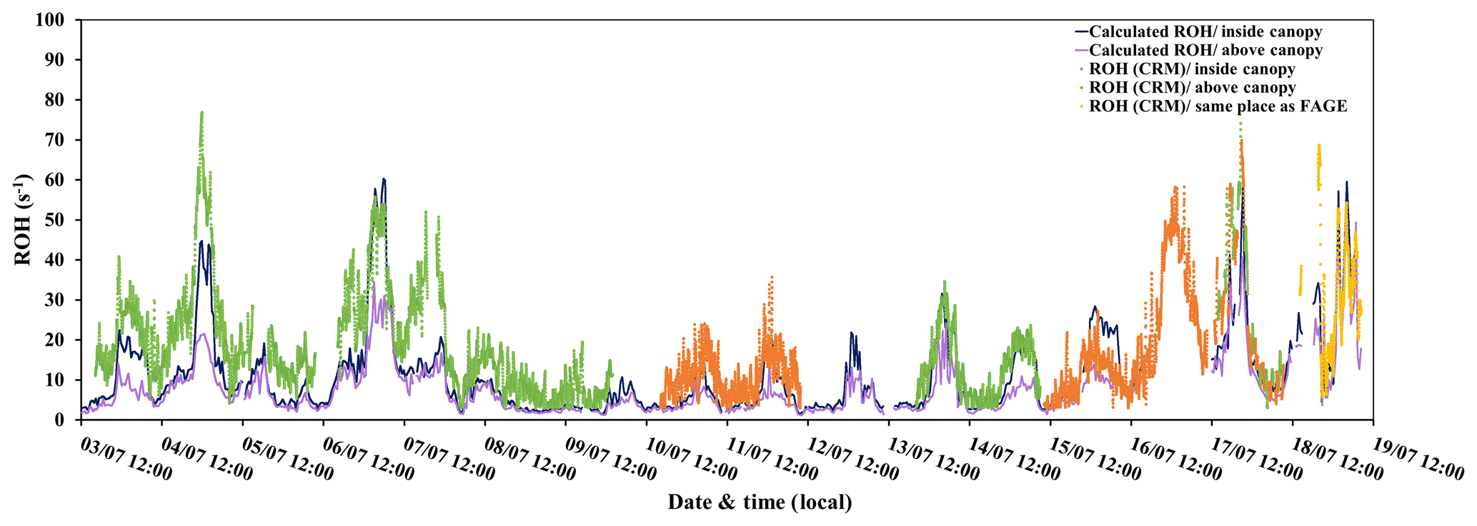
Figure 6Variability of measured ROH (LSCE-CRM) and calculated ROH (PTR-MS) at 6 and 12 m of height.
In the end, even though BVOC emissions are more intense during the day (Simon et al., 1994), the higher turbulence observed compared to nighttime led to a faster mixing within the canopy and thus similar levels of isoprene and monoterpenes inside and above the canopy. These daytime levels were lower than those observed at night for monoterpenes and higher for isoprene, the latter being light and temperature dependent.
To conclude, these observations show that, on one hand, lower turbulence inducing stable atmospheric conditions during the night explains the observed stratification in terms of monoterpene levels and thus in terms of OH reactivity levels within the canopy; on the other hand, higher turbulence during daytime leads to higher mixing within the canopy and vertical homogeneity, with similar BVOC concentrations and OH reactivity levels at both heights. Diurnal average values of total OH reactivity for inside- and above-canopy measurements are given in Table S9.
3.3 Measured and calculated ROH within and above the canopy
Figure 6 shows that there is a good covariation of the measured total OH reactivity by the CRM instrument with the values calculated from the PTR-MS data (22 %–24 % (2σ)). However, a certain fraction of the measured total OH reactivity remains unexplained by the considered compounds (Table 3). Diurnal variations of OH reactivity were observed within the canopy during the major part of the campaign, with maximum values recorded during most nights and averages of 19.2±12.8 and 19.3±16.3 s−1 measured by the LSCE-CRM and UL-FAGE instruments, respectively. This diurnal cycle was also observed above the canopy where the average total OH reactivity was 16.5±12.3 s−1, which is higher than observations made in other temperate coniferous forests (Ramasamy et al., 2016) where the reported OH reactivity ranges from 4 to 13 s−1 (campaign average).
During the first part of the campaign (3–10 July), when the LSCE-CRM was measuring alone inside the canopy, total OH reactivity varied between LOD (3 s−1 at 3σ) and 76.9 s−1, while the calculated reactivity ranged between 1.4 and 60 s−1. During the second period (13–15 and 17–18 July), similar maxima were recorded by the LSCE-CRM (74.2 s−1) and the UL-FAGE instruments (78.9 s−1), when both were measuring at two different locations within the canopy. Regarding the calculated OH reactivity, it varied between 2.6 and 59.3 s−1. During this same period, the FAGE instrument measured alone within the canopy from 15 to 17 July and recorded total OH reactivity values ranging between 3.6 and 99.2 s−1; however, the PTR-MS data were not taken into account for the period from 16 July 15:00 LT to 17 July 12:00 LT due to an electrical failure. Finally, during the last 2 d (18–19 July), total OH reactivity showed a particular behavior as mentioned in Sect. 3.2. It started to increase in the afternoon, reached a maximum at the beginning of the night, which was suddenly broken by turbulences, and showed three peaks during the night corresponding to more stable conditions observed for both the measured and calculated reactivity.
Regarding above-canopy measurements, the measured OH reactivity varied between LOD and 35.7 s−1 between 10 and 12 July, whereas the calculated reactivity varied between 1.2 and 14.5 s−1. A similar trend was observed for the second period of measurements performed above the canopy (15–18 July) during which higher OH reactivity was recorded with a maximum of 69.9 s−1, which is 1.7 times higher than the calculated OH reactivity (40.8 s−1).
3.4 Contribution of VOCs (PTR-MS) to calculated OH reactivity within and above the canopy
Figure 7 shows the breakdown of trace gases to the calculated OH reactivity during daytime and nighttime at the two heights, taking into account the whole measurement period (campaign average). We note that primary BVOCs (monoterpenes, isoprene) are by far the main contributors to the calculated OH reactivity, representing 92 %–96 % of the calculated OH reactivity on average.
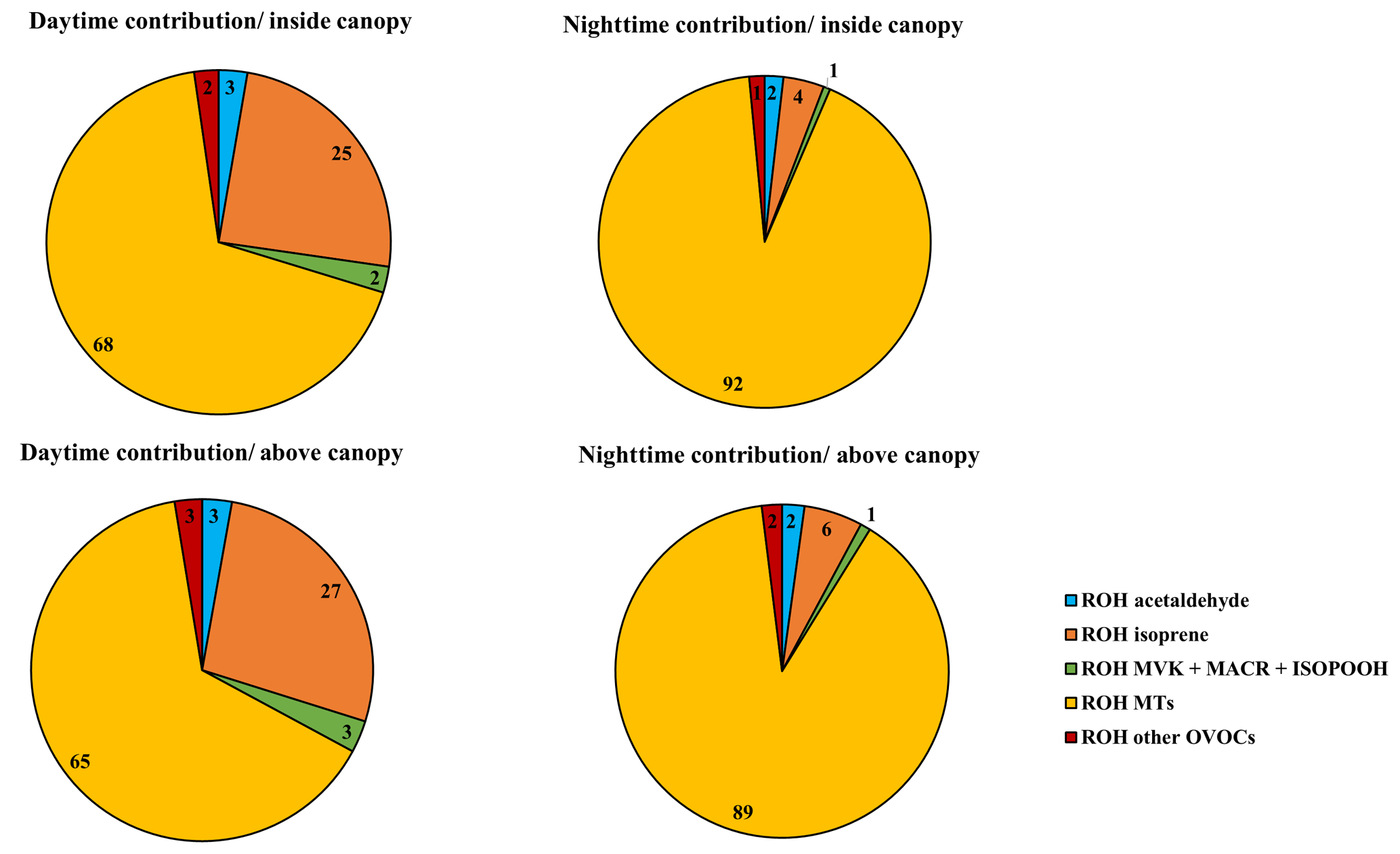
Figure 7The components of calculated OH reactivity within and above the canopy during daytime and nighttime.
Monoterpenes exhibited the most prominent contribution to the calculated OH reactivity. These species had a similar contribution within and above the canopy but significant differences between daytime (68 %–65 %) and nighttime (92 %–89 %). Next to monoterpenes, isoprene had a maximum contribution during daytime and represented on average 25 %–27 % of the calculated OH reactivity, followed by acetaldehyde (3 %) and MACR + MVK + ISOPOOH (2 %–3 %) at both measurement heights. However, during nighttime, isoprene accounted for only 4 %–6 % of the OH reactivity measured within and above the canopy, with acetaldehyde contributing approximately 2 % and MACR + MVK + ISOPOOH around 1 %.
Thus, we can conclude that no substantial difference in the atmospheric chemical composition existed between the two sampling heights, even when we only consider stable nights (the monoterpene relative contribution is around 92 % inside and above the canopy).
3.5 Description and investigation of potential missing OH reactivity during the LANDEX campaign
The missing OH reactivity was calculated as a difference between the total OH reactivity measured by LSCE-CRM, since it was operated over the whole campaign and at both heights, and the OH reactivity calculated from PTR-MS data. It is worth noting that a scatter plot of the LSCE-CRM and UL-FAGE data led to a slope of 1.28 and an intercept of 0.96 s−1 (Sect. 3.1.1), indicating higher OH reactivity values measured by the CRM instrument. Considering OH reactivity values measured by the CRM instrument may therefore maximize the missing OH reactivity. In the following, the analysis of the missing OH reactivity was performed when it was higher than both the LOD of 3 s−1 (3σ) and 35 % of the measured OH reactivity (uncertainty on the CRM measurements; see Sect. 2.2).
Figure 8 shows (a) the variability of the missing OH reactivity within and above the canopy, together with ambient temperature, (b) friction velocity (red), and ozone mixing ratios within (yellow) and above (blue) the canopy. The ozone variability is discussed below as ozone chemistry can dominate the nighttime chemistry of BVOCs observed at this site (σ-pinene, β-pinene) (Fuentes et al., 2002; Kammer et al., 2018).
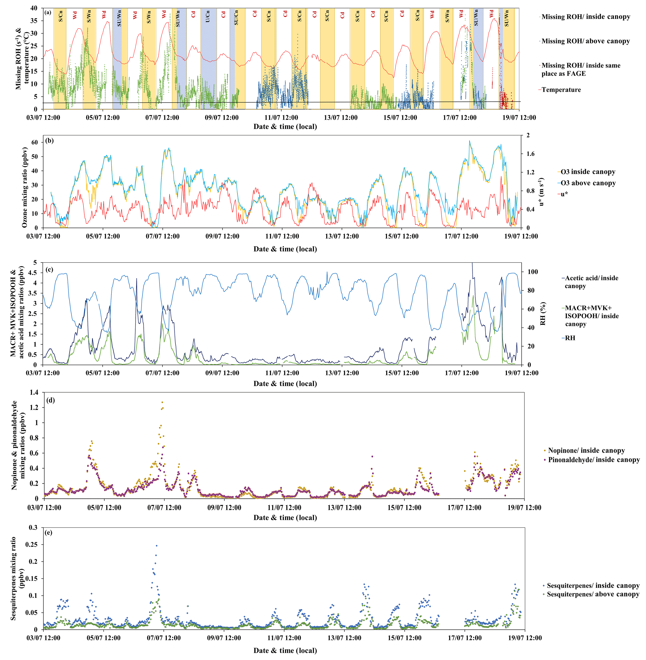
Figure 8Missing OH reactivity inside and above the canopy together with (a) temperature, (b) friction velocity (red), ozone mixing ratios inside (yellow) and above (blue) the canopy, (c) relative humidity (clear blue), MACR + MVK + ISOPOOH (dark blue) and acetic acid (green) inside the canopy, (d) nopinone (yellow) and pinonaldehyde (purple) inside the canopy, and (e) sesquiterpenes inside (blue) and above (green) the canopy.
The concentration of OH was 4.2×10⁶ molecules cm−3 on average during daytime, with a maximum of 4.3×10⁷ molecules cm−3, and around 1.5×10⁶ molecules cm−3 on average during nighttime (data available between 13 and 19 July). However, a potential artifact on OH radical measurements, leading to a possible overestimation of OH radical concentrations, could not be ruled out. Regarding ozone, its mixing ratio showed a diurnal cycle with maximum values during the day (max ≈ 60 ppbv, mean ≈ 29 ppbv) that were similar within and above the canopy due to efficient mixing and lower levels during nights, with an average of 18 ppbv inside the canopy, while levels were higher by 1–10 ppbv on average above the canopy. Considering OH and O3 average mixing ratios, the α-pinene lifetime was estimated to be 1.2 and 4 h, respectively, during the day and 3.6 and 5.8 h, respectively, during the night. At maximum OH and O3 mixing ratios during daytime, the α-pinene lifetime was reduced to 7.4 min and 2 h, respectively. Thus, OH chemistry remained dominant compared to the ozonolysis of the main emitted compounds at this site (i.e., α-pinene). An article on the reactivity of monoterpenes with OH, ozone and nitrate for this campaign is in preparation (Kenneth Mermet, personal communication, 2019).
When comparing measurements of OH reactivity with calculations based on PTR-MS data (see Table 3), an average of 38 % (7.2 s−1) and 48 % (6.1 s−1) remained unexplained inside and above the canopy, respectively.
Considering other measurements performed inside the canopy (6 m) and not included in the OH reactivity calculations, such as NO, NO2, ozone and butanol (leakage from SMPS), and assuming constant concentrations of CO (150 ppbv) and methane (2000 ppbv), their contribution can reach 3.0 s−1 on average (maximum around 7 s−1) at this level. This said, the mean missing OH reactivity was finally around 4.2 s−1 (22 %) inside the canopy for the whole measurement period.
Regarding other measurements performed above the canopy, online chromatographic instruments (Table 3) provided information on other oxygenated VOCs (seven compounds) and non-methane hydrocarbons (36 compounds). These compounds could explain 0.48 s−1 on average (0.43 s−1 from NMHC and 0.05 s−1 from OVOC measured by GC) of the missing OH reactivity between 10 and 12 July. However, after 14 July, the GC measuring OVOC stopped working, but NMHCs alone could account for 0.5 s−1 of missing OH reactivity on average. While O3 was measured at 12 m, no NOx measurements were performed at this height; however, their contribution at the 6 m height was 0.3 s−1 on average, suggesting only a small contribution to the missing OH reactivity. Methane and CO were also considered, assuming the same mixing ratios as inside. Finally, looking at butanol measured by the PTR-MS at the 12 m height, a maximum mean contribution of 0.3 s−1 was assessed for the nights of 10–11 July. Hence, considering OVOCs, NMHC, O3, CO, CH4 and butanol, the mean missing OH reactivity above the canopy level was around 4.3 s−1 (33 %). However, this missing fraction exhibited a diurnal variability at both heights, which is worth discussing in detail. A summary of mean missing OH reactivity values at both heights is presented in Table 4.
Table 4Summary of the measured OH reactivity and the missing OH reactivity inside and above the canopy during the day and the night, taking into account only PTR-MS data or all the data available at each height for OH reactivity calculations. These averages are calculated for the periods when CRM, PTR-MS and other instrumental data are available.
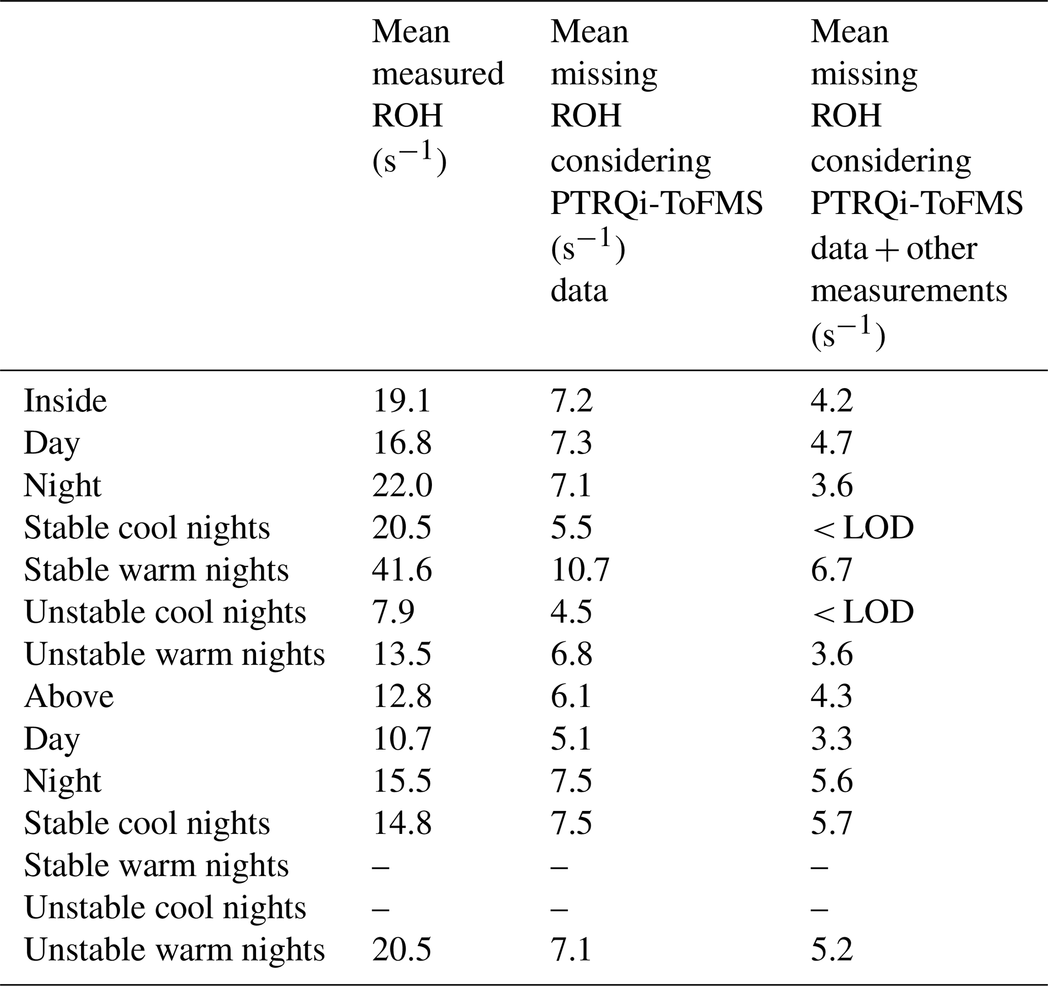
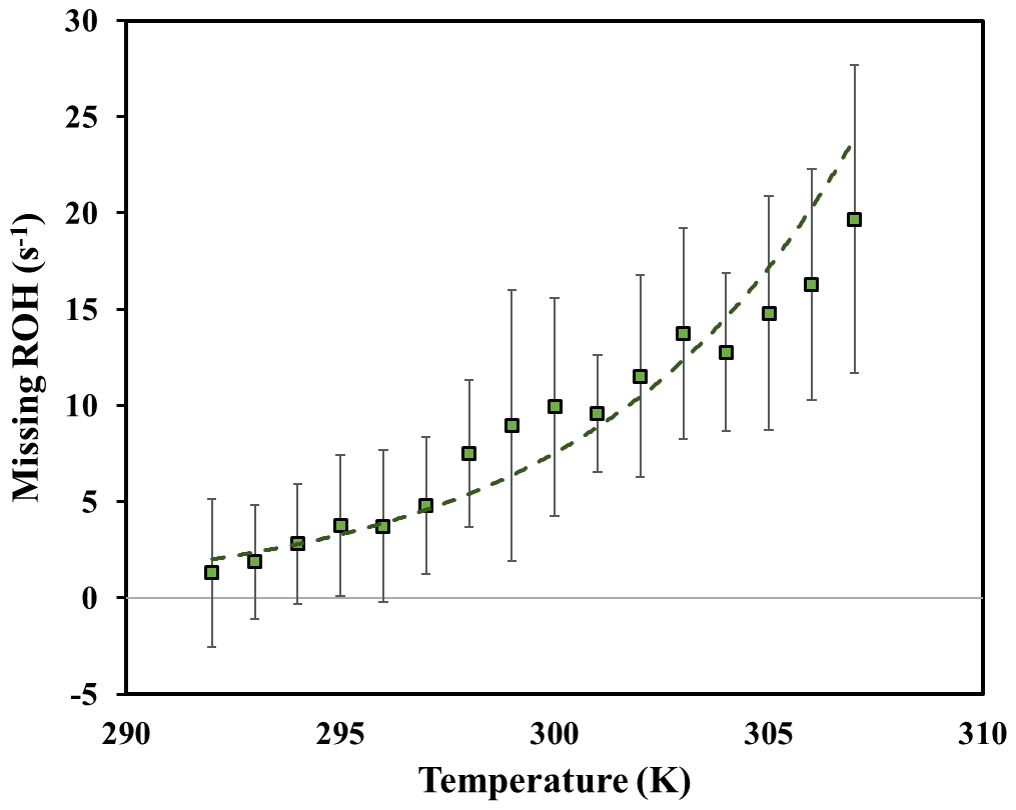
Figure 9Daytime missing OH reactivity binned by ambient temperature for the 6 m height for temperatures ranging from 292 to 308 K. Error bars represent the standard deviation on missing OH reactivity calculated for each temperature bin.
3.5.1 Daytime missing OH reactivity
Analyzing the behavior of missing OH reactivity during daytime for inside-canopy measurements, Fig. 9 shows that it increases exponentially with temperature. Indeed, the average missing OH reactivity was around 7.5 s−1 for Wd days, after taking into account other available measurements at this height (NO, NO2, O3, butanol, and estimated CO and CH4), whereas no missing reactivity was seen for cooler days (< LOD). As reported in Di Carlo et al. (2004), the missing OH reactivity was fitted with an equation usually used to describe temperature-dependent emissions of monoterpenes (Guenther et al., 1993): , where E(T) and E(293) represent the emission rate at a given temperature T and at 293 K, respectively. In this equation, E(T) was substituted by MROH(T) and E(293) by MROH(293), with MROH representing the missing OH reactivity (Hansen et al., 2014). The value of β determined from the fit of the data for the 6 m height (daytime) is around 0.17, higher than the values attributed to monoterpene emissions from vegetation (0.057 to 0.144 K−1). Higher β values were also obtained by Mao et al. (2012), Hansen et al. (2014) and Kaiser et al. (2016), wherein they suggested that daytime missing reactivity is mostly linked to secondary oxidation products. However, the use of the β factor must be done with caution, as the missing OH reactivity can be influenced by processes that do not affect BVOCs emissions (i.e., the boundary layer height and vertical mixing). Furthermore, we cannot exclude the possibility of light- and temperature-dependent emissions. Indeed, Kaiser et al. (2016) also investigated the temperature dependency of daytime missing OH reactivity in an isoprene-dominated forest, reporting that part of the missing emissions could be characterized by a light and temperature dependence, knowing that temperature increases with increasing solar radiation. Above the canopy, most measurements were performed during cool days. Thus, it was not possible to analyze the temperature dependence of above-canopy daytime missing OH reactivity.
Another way to investigate the origin of missing OH reactivity is by examining its covariability with compounds such as acetic acid and MACR + MVK + ISOPOOH, knowing that MACR and MVK are oxidation products of isoprene. First, for the higher daytime missing OH reactivity observed for Wd days (within and above the canopy), Fig. 8c shows that the missing reactivity increases with acetic acid (mixing ratio up to 5 ppbv). Acetic acid can be directly emitted by the trees and the soil (Kesselmeier and Staudt, 1999) and could also be an oxidation product of BVOCs, including isoprene (Paulot et al., 2011). This compound showed a diurnal cycle similar to that of isoprene (Fig. 5c) and was not used to calculate the OH reactivity. Despite its relatively low reactivity with OH, this compound showed a maximum calculated OH reactivity during Wd days that was, on average (0.07 s−1), 4 times higher than that of Cd days. Thus, it could explain, with other compounds exhibiting a similar temporal behavior, part of the missing OH reactivity seen during warm days. MACR + MVK + ISOPOOH showed a general trend, with higher values during the day and lower values during the night, suggesting that the oxidation products of isoprene could be responsible for the daytime missing OH reactivity. These levels were generally higher for Wd days than for Cd, reflecting a higher yield of secondary products and more intense photochemistry during warm days.
3.5.2 Nighttime missing OH reactivity
On average, the highest nighttime missing OH reactivity inside the canopy (13.1 s−1) was observed on the stable and warm night of 4–5 July, whereas during stable and cool as well as unstable and warm nights, no significant missing OH reactivity was found (< LOD). Interestingly, the stable and warm night of 6–7 July did not show significant missing OH reactivity, meaning that the missing fraction inside the canopy during night was not only influenced by meteorological parameters, even if, as shown before, BVOC concentrations and total OH reactivity were. So what was the difference between these two nights with similar meteorological conditions?
Checking monoterpene oxidation product variabilities (nopinone and pinonaldehyde), both nights exhibited higher concentration levels of these species; however, their contribution to OH reactivity remained relatively low and did not exceed 1 s−1 on average for both nights, keeping in mind that this is a lower limit of their contribution (since the reported measurements do not account for potential fragmentation in the PTR-MS). Thus, only a small part of the missing fraction can be explained by these species. Interestingly, isoprene, acetic acid and MVK + MACR + ISOPOOH exhibited higher concentration levels during the night of 4–5 July, which was not the case for the night of 6–7 July. Indeed, these species marked relatively high nocturnal and inside-canopy levels. When looking at air mass backward trajectories (Fig. 10), the night of 4–5 July was characterized by an air mass originally coming from the ocean, which spent at least 48 h above the continent before reaching the site. This could have led to the enrichment of the air mass with species emitted by the widely spread Landes forests and their oxidation products. Thus, the significant missing OH reactivity observed during the mentioned night is likely related to unconsidered compounds of biogenic origin characterized by a similar behavior to that of isoprene, acetic acid and MVK + MACR + ISOPOOH, which accumulated in the stable nocturnal boundary layer. In contrast, air masses spent approximately 12–18 h above the continent during 6–7 July, with more time above the ocean. Marine air masses are generally known to be clean, with relatively low levels of reactive species. Even though the night of 5–6 July shows similar air mass backward trajectories to the night of 4–5 July, the higher turbulence during this night prevents the accumulation of reactive species (including long-lived oxidation products) due to a higher boundary layer height, lowering the reactivity and the missing OH reactivity (Fig. 10).
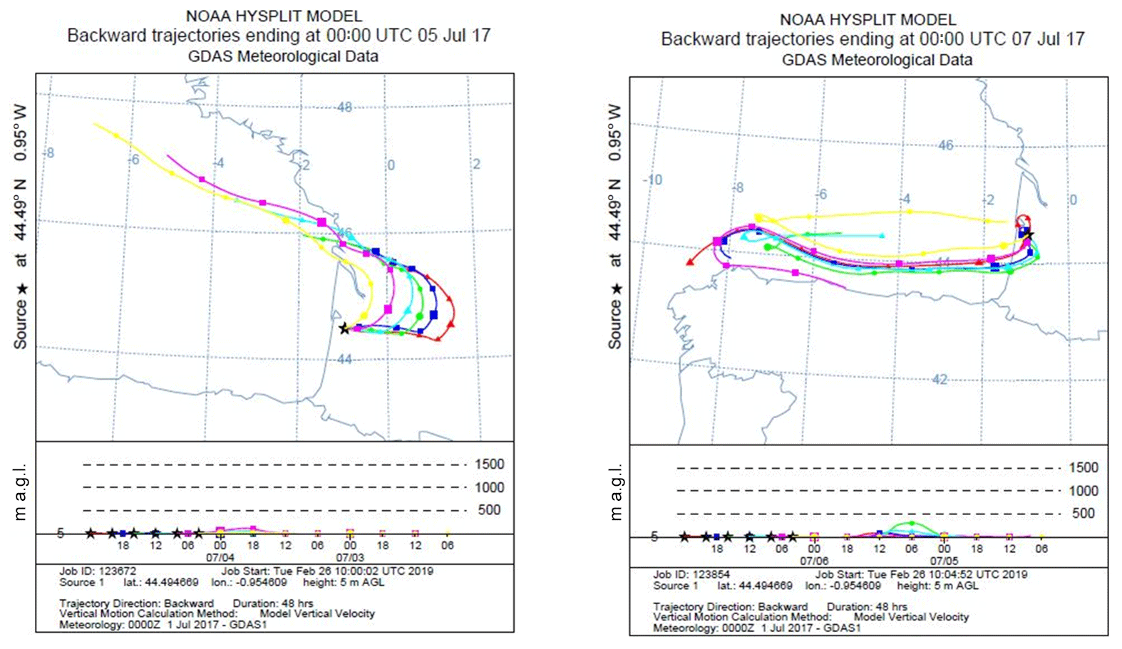
Figure 10Air mass backward trajectories for the nights of 4–5 and 6–7 July. Red lines represent air masses arriving around midnight UTC (around 02:00 LT – local time) to the site. The time difference between two points is 6 h.
Regarding above-canopy measurements (10–12 and 15–18 July), the nighttime average missing OH reactivity was 5.6 s−1 (all the nights were characterized by stable and cool atmospheric conditions). Monoterpene oxidation products had similar concentration levels above and inside the canopy. Their maximum contribution was around 0.4 s−1 on average for the SU/W night of 17–18 July. Therefore, these monoterpene nighttime oxidation products are only responsible for a small fraction of the missing OH reactivity observed above the canopy during the night. Sesquiterpenes (SQTs) exhibited a similar temporal trend as monoterpenes, showing higher mixing ratios during nighttime. Interestingly, sesquiterpene mixing ratios were higher inside the canopy compared to above and the difference was significant during stable nights. O3 mixing ratios during these nights decreased to very low levels. Plotting the ratio SQT(above) ∕ MTs(above) with the ratio SQT(inside) ∕ MTs(inside) shows a good linear correlation with a slope of 0.73 and an R2 of 0.6. Knowing that sesquiterpenes are highly reactive with ozone (Ciccioli et al., 1999), which can dominate the chemistry during dark hours, this observation suggests that a larger fraction of these species (≈30 %) could be consumed by ozonolysis above the canopy, leading to the formation of unidentified secondary compounds. However, sesquiterpenes were present at relatively low concentrations (maximum of 0.25 and 0.11 ppbv inside and above the canopy, respectively). Assuming that all sesquiterpenes are β-caryophyllene and considering that 30 % are transformed into first-generation oxidation products through ozonolysis reactions, the maximum mixing ratio of these products would be around 0.07 ppbv each, assuming a yield of 1. However, it was reported by Winterhalter et al. (2009) that oxidation products of β-caryophyllene were much less reactive (100 times) than their precursor. Thus, the contribution of sesquiterpene nighttime oxidation products to the missing OH reactivity is likely negligible.
Finally, it is worth noting that Holzinger et al. (2005) reported the emission of highly reactive BVOCs in a coniferous forest, which is 6–30 times the emission of monoterpenes in the studied Ponderosa pine forest. This large fraction of BVOCs is subject to oxidation by ozone and OH, leading to unidentified, non-accounted for secondary molecules. These oxidation products can participate in the growth of new particles. Indeed, new particle formation episodes were recently reported on this site (Kammer et al., 2018).
To summarize, higher daytime missing OH reactivity was observed for warm days (Wd) inside and above the canopy, exhibiting a dependency on temperature profiles and showing that trace gases leading to the missing OH reactivity could be linked to an enhancement of primary species as well as secondary product formation. Regarding nighttime missing OH reactivity, higher levels were seen for the stable and warm night of 4–5 July, showing that these conditions could have been favorable for the accumulation of long-lived species (primary and secondary species) during the transport of the air mass from nearby forests.
During summer 2017, total OH reactivity measurements were conducted as part of the LANDEX field campaign in the Landes maritime pine forest (France). During this campaign, two instruments (LSCE-CRM and UL-FAGE) were deployed to measure total OH reactivity inside and above the canopy as well as at two different locations inside the canopy level. The comparison between the two instruments, based on measurements done at the same location at the end of the campaign, showed a good agreement within instrument uncertainties (slope of 1.28 on a linear correlation plot). Measuring at two different locations demonstrated a good horizontal homogeneity inside the canopy, even during episodes of vertical stratification that were observed during some nights.
Total OH reactivity recorded an average of 19.2 s−1 at 6 m of height, 1.2 times higher than that observed above the canopy level at 12 m of height. It varied similarly at both heights, following a diurnal cycle with two maxima, one during daytime following isoprene's profile and a higher one during nighttime when monoterpene concentrations reached their maxima. The latter were the main emitted compounds in this forest ecosystem.
The variability of BVOC concentrations and OH reactivity was strongly dependant on meteorological parameters. Daytime OH reactivity was linked to ambient temperatures and light, two parameters governing the emissions of temperature- and/or light-dependent compounds (like isoprene), whereas nighttime OH reactivity was influenced by nighttime temperatures and vertical turbulence intensity. Indeed, low turbulence, high temperature and lower oxidation rates than during daytime led to higher concentrations of monoterpenes and thus higher OH reactivity during stable and warm nights. In addition, higher differences in BVOC levels and total OH reactivity were observed between the two studied heights, particularly during stable nights.
Furthermore, monoterpenes were shown to be the main contributors to total OH reactivity during both daytime and nighttime. These species accounted for more than 60 % of the OH reactivity during daytime, followed by isoprene (25 %–27 %), acetaldehyde (3 %) and MACR + MVK + ISOPOOH (2 %–3 %). However, the contributions of isoprene and OVOCs were much lower at both levels during the night, leading to a higher contribution of monoterpenes, which was slightly more important inside the canopy level due to the stratified conditions.
An investigation of the missing OH reactivity indicated averages of 22 % and 33 % inside and above the canopy, respectively, over the whole campaign when comparing the measured OH reactivity to the calculated one from PTR-MS and other available measurements. However, it showed some diurnal variability at both heights. During daytime, higher missing OH reactivity was observed on warmer days inside and above the canopy. Plotted against temperature, inside-canopy missing OH reactivity showed a dependency on temperature. The analysis suggested that the missing OH reactivity may be due to unmeasured primary emitted compounds and oxidation products. In this context, OH reactivity measurements from a Pinus pinaster Aiton branch enclosure could be of great interest to verify the contribution of unaccounted for or unmeasured BVOC emissions to OH reactivity, as done by Kim et al. (2011) for red oak and white pine branch enclosures. Furthermore, higher levels of isoprene oxidation products on warmer days also suggest that the missing reactivity could be due to the formation of unmeasured oxidation products. Regarding the nighttime period, the highest missing OH reactivity was found inside the canopy for the night of 4–5 July. This night was characterized by higher levels of isoprene and its oxidation products compared to the night of 6–7 July with similar atmospheric conditions. Air mass backward trajectories showed a continental origin for this night, suggesting that species emitted by the largely spread Landes forest could have been imported to the site and accumulated due to the stable nocturnal boundary layer. These species, unmeasured by the deployed analytical instruments and hence not considered in OH reactivity calculations, could explain the higher missing OH fraction for the night of 4–5 July. The investigation of sesquiterpene and monoterpene oxidation products (nopinone and pinonaldehyde) measured by PTR-MS highlighted their small contribution in terms of OH reactivity. They only explained a small fraction of the observed missing OH reactivity inside and above the canopy during night. Finally, given the time needed and the data required, no modeling study was performed; however, it would be interesting to run a box model in order to get more insights into the origin of the missing OH reactivity.
Data are available upon request from the corresponding author.
The supplement related to this article is available online at: https://doi.org/10.5194/acp-20-1277-2020-supplement.
SB and FT set up and carried out OH reactivity measurements with the LSCE-CRM. MAA, CS, SB and CH set up and carried out OH reactivity measurements with the UL-FAGE instrument. KM, TL, SS and NL carried out GC-BVOC2, GC-OVOC and GC-NMHC measurements and provided analyzed data. VG provided GC-BVOC1 analyzed data. SD carried out PTR-MS measurements and provided the corresponding data. JK and PMF provided NOx data and meteorological parameters. EV, EP and PMF coordinated the LANDEX project and field campaign. SB prepared the paper with coauthor contributions, mainly MAA, CS, DD and VG.
The authors declare that they have no conflict of interest.
The authors want to acknowledge the Bilos ICOS team for meteorological data and site availability as well as Ineris for sharing their mobile laboratory. We would like to thank Sébastien Schramm, Dominique Baisnée and Roland Sarda-Esteve for their help during the installation of the PTR-Quad-MS and the GC-FID. We are also thankful to Jean-Yves Peterschmitt for his help with the orthogonal distance regression technique using Python.
This study was supported by the European Union's Horizon 2020 research and innovation program under Marie Skłodowska-Curie grant agreement no. 674911-IMPACT, ADEME-LANDEX and the CNRS. The PC2A and SAGE participation was supported by the French ANR agency under contract no. ANR-11-LabX-0005-01 CaPPA (Chemical and Physical Properties of the Atmosphere), the Région Hauts-de-France, the Ministère de l'Enseignement Supérieur et de la Recherche (CPER Climibio) and the European Fund for Regional Economic Development.
This paper was edited by Dwayne Heard and reviewed by three anonymous referees.
ACTRIS: WP4-NA4: Trace gases networking: Volatile organic carbon and nitrogen oxides, Deliverable D4.9, Final SOPs for VOCs measurements, Final Version, available at: http://www.actris.eu/Portals/46/Data and Services/Measurement guidelines/Near-surface trace gases/ACTRIS-1 Deliverable_WP4_D4.9_M42_v2_Sep2014.pdf?ver=2017-03-20-135044- (last access: 23 January 2020), 2014.
Amedro, D., Miyazaki, K., Parker, A., Schoemaecker, C., and Fittschen, C.: Atmospheric and kinetic studies of OH and HO2 by the FAGE technique, J. Environ. Sci., 24, 78–86, https://doi.org/10.1016/S1001-0742(11)60723-7, 2012.
Atkinson, R.: Kinetics and Mechanisms of the Gas-Phase Reactions of the Hydroxyl Radical with Organic Compounds under Atmospheric Conditions, Chem. Rev., 85, 69–201, https://doi.org/10.1021/cr00063a002, 1985.
Atkinson, R. and Arey, J.: Gas-phase tropospheric chemistry of biogenic volatile organic compounds: A review, Atmos. Environ., 37, 197–219, https://doi.org/10.1016/S1352-2310(03)00391-1, 2003.
Atkinson, R., Baulch, D. L., Cox, R. A., Crowley, J. N., Hampson, R. F., Hynes, R. G., Jenkin, M. E., Rossi, M. J., Troe, J., and IUPAC Subcommittee: Evaluated kinetic and photochemical data for atmospheric chemistry: Volume II – gas phase reactions of organic species, Atmos. Chem. Phys., 6, 3625–4055, https://doi.org/10.5194/acp-6-3625-2006, 2006.
Badol, C., Borbon, A., Locoge, N., Léonardis, T., and Galloo, J. C.: An automated monitoring system for VOC ozone precursors in ambient air: Development, implementation and data analysis, Anal. Bioanal. Chem., 378, 1815–1827, https://doi.org/10.1007/s00216-003-2474-0, 2004.
Brune, W. H., Singh, H. B., Cohen, R. C., Hall, S. R., Olson, J. R., Diskin, G. S., Heikes, B., Sachse, G. W., Crawford, J. H., Ren, X., Blake, D. R., Huey, L. G., Shetter, R. E., Mao, J., and Fried, A.: Airborne measurement of OH reactivity during INTEX-B, Atmos. Chem. Phys., 9, 163–173, https://doi.org/10.5194/acp-9-163-2009, 2010.
Ciccioli, P., Brancaleoni, E., Frattoni, M., Di Palo, V., Valentini, R., Tirone, G., Seufert, G., Bertin, N., Hansen, U., Csiky, O., Lenz, R., and Sharma, M.: Emission of reactive terpene compounds from orange orchards and their removal by within-canopy processes, J. Geophys. Res.-Atmos., 104, 8077–8094, https://doi.org/10.1029/1998JD100026, 1999.
Di Carlo, P., Brune, W. H., Martinez, M., Harder, H., Lesher, R., Ren, X., Thornberry, T., Carroll, M. A., Young, V., Shepson, P. B., Riemer, D., Apel, E., and Campbell, C.: Missing OH Reactivity in a Forest: Evidence for Unknown Reactive Biogenic VOCs, Science, 304, 722–725, https://doi.org/10.1126/science.1094392, 2004.
Dolgorouky, C., Gros, V., Sarda-Esteve, R., Sinha, V., Williams, J., Marchand, N., Sauvage, S., Poulain, L., Sciare, J. and Bonsang, B.: Total OH reactivity measurements in Paris during the 2010 MEGAPOLI winter campaign, Atmos. Chem. Phys., 12, 9593–9612, https://doi.org/10.5194/acp-12-9593-2012, 2012.
Dusanter, S. and Stevens, P.: Recent Advances in the Chemistry of OH and HO2 Radicals in the Atmosphere: Field and Laboratory Measurements, Advances in Atmospheric Chemistry, World Scientific Publishing Company Incorporated, p. 72, 2017.
Edwards, P. M., Evans, M. J., Furneaux, K. L., Hopkins, J., Ingham, T., Jones, C., Lee, J. D., Lewis, A. C., Moller, S. J., Stone, D., Whalley, L. K., and Heard, D. E.: OH reactivity in a South East Asian tropical rainforest during the oxidant and particle photochemical processes (OP3) project, Atmos. Chem. Phys., 13, 9497–9514, https://doi.org/10.5194/acp-13-9497-2013, 2013.
Fuchs, H., Novelli, A., Rolletter, M., Hofzumahaus, A., Pfannerstill, E. Y., Kessel, S., Edtbauer, A., Williams, J., Michoud, V., Dusanter, S., Locoge, N., Zannoni, N., Gros, V., Truong, F., Sarda-Esteve, R., Cryer, D. R., Brumby, C. A., Whalley, L. K., Stone, D., Seakins, P. W., Heard, D. E., Schoemaecker, C., Blocquet, M., Coudert, S., Batut, S., Fittschen, C., Thames, A. B., Brune, W. H., Ernest, C., Harder, H., Muller, J. B. A., Elste, T., Kubistin, D., Andres, S., Bohn, B., Hohaus, T., Holland, F., Li, X., Rohrer, F., Kiendler-Scharr, A., Tillmann, R., Wegener, R., Yu, Z., Zou, Q., and Wahner, A.: Comparison of OH reactivity measurements in the atmospheric simulation chamber SAPHIR, Atmos. Meas. Tech., 10, 4023–4053, https://doi.org/10.5194/amt-10-4023-2017, 2017.
Fuentes, J. D., Lerdau, M., Atkinson, R., Baldocchi, D., Bottenheim, J. W., Ciccioli, P., Lamb, B., Geron, C., Gu, L., Guenther, A., Sharkey, D., and Stockwellk, W.: Biogenic Hydrocarbons in the Atmospheric Boundary Layer: A Review, B. Am. Meteorol. Soc., 81, 1537–1575, https://doi.org/10.1175/1520-0477(2000)081<1537:bhitab>2.3.co;2, 2002.
Gros, V., Gaimoz, C., Herrmann, F., Custer, T., Williams, J., Bonsang, B., Sauvage, S., Locoge, N., d'Argouges, O., Sarda-Estève, R., and Sciare, J.: Volatile organic compounds sources in Paris in spring 2007. Part I: qualitative analysis, Environ. Chem., 8, 74–90, https://doi.org/10.1071/en10068, 2011.
Guenther, A., Hewitt, C. N., Erickson, D., Fall, R., Geron, C., Graedel, T., Harley, P., Klinger, L., Lerdau, M., McKay, W. A., Pierce, T., Scholes, B., Steinbrecher, R., Tallamraju, R., Taylor, J., and Zimmerman, P.: A global model of natural volatile organic compound emissions, J. Geophys. Res., 100, 8873, https://doi.org/10.1029/94JD02950, 1995.
Guenther, A. B., Zimmerman, P. R., Harley, P. C., Monson, R. K., and Fall, R.: Isoprene and monoterpene emission rate variability: model evaluations and sensitivity analyses, J. Geophys. Res., 98, 12609, https://doi.org/10.1029/93jd00527, 1993.
Hansen, R. F., Griffith, S. M., Dusanter, S., Rickly, P. S., Stevens, P. S., Bertman, S. B., Carroll, M. A., Erickson, M. H., Flynn, J. H., Grossberg, N., Jobson, B. T., Lefer, B. L., and Wallace, H. W.: Measurements of total hydroxyl radical reactivity during CABINEX 2009 – Part 1: Field measurements, Atmos. Chem. Phys., 14, 2923–2937, https://doi.org/10.5194/acp-14-2923-2014, 2014.
Hansen, R. F., Blocquet, M., Schoemaecker, C., Léonardis, T., Locoge, N., Fittschen, C., Hanoune, B., Stevens, P. S., Sinha, V., and Dusanter, S.: Intercomparison of the comparative reactivity method (CRM) and pump–probe technique for measuring total OH reactivity in an urban environment, Atmos. Meas. Tech., 8, 4243–4264, https://doi.org/10.5194/amt-8-4243-2015, 2015.
Holzinger, R., Lee, A., Paw, K. T., and Goldstein, U. A. H.: Observations of oxidation products above a forest imply biogenic emissions of very reactive compounds, Atmos. Chem. Phys., 5, 67–75, https://doi.org/10.5194/acp-5-67-2005, 2005.
Ingham, T., Goddard, A., Whalley, L. K., Furneaux, K. L., Edwards, P. M., Seal, C. P., Self, D. E., Johnson, G. P., Read, K. A., Lee, J. D., and Heard, D. E.: A flow-tube based laser-induced fluorescence instrument to measure OH reactivity in the troposphere, Atmos. Meas. Tech., 2, 465–477, https://doi.org/10.5194/amt-2-465-2009, 2009.
Kaiser, J., Skog, K. M., Baumann, K., Bertman, S. B., Brown, S. B., Brune, W. H., Crounse, J. D., de Gouw, J. A., Edgerton, E. S., Feiner, P. A., Goldstein, A. H., Koss, A., Misztal, P. K., Nguyen, T. B., Olson, K. F., St. Clair, J. M., Teng, A. P., Toma, S., Wennberg, P. O., Wild, R. J., Zhang, L., and Keutsch, F. N.: Speciation of OH reactivity above the canopy of an isoprene-dominated forest, Atmos. Chem. Phys., 16, 9349–9359, https://doi.org/10.5194/acp-16-9349-2016, 2016.
Kammer, J., Perraudin, E., Flaud, P. M., Lamaud, E., Bonnefond, J. M., and Villenave, E.: Observation of nighttime new particle formation over the French Landes forest, Sci. Total Environ., 621, 1084–1092, https://doi.org/10.1016/j.scitotenv.2017.10.118, 2018.
Kari, E., Miettinen, P., Yli-Pirilä, P., Virtanen, A., and Faiola, C. L.: PTR-ToF-MS product ion distributions and humidity-dependence of biogenic volatile organic compounds, Int. J. Mass Spectrom., 430, 87–97, https://doi.org/10.1016/j.ijms.2018.05.003, 2018.
Kesselmeier, J. and Staudt, M.: Biogenic volatile organic compounds (VOC): An overview on emission, physiology and ecology, J. Atmos. Chem., 33, 23–88, https://doi.org/10.1023/A:1006127516791, 1999.
Kim, S., Karl, T., Helmig, D., Daly, R., Rasmussen, R., and Guenther, A.: Measurement of atmospheric sesquiterpenes by proton transfer reaction-mass spectrometry (PTR-MS), Atmos. Meas. Tech., 2, 99–112, https://doi.org/10.5194/amt-2-99-2009, 2009.
Kim, S., Guenther, A., Karl, T., and Greenberg, J.: Contributions of primary and secondary biogenic VOC tototal OH reactivity during the CABINEX (Community Atmosphere-Biosphere INteractions Experiments)-09 field campaign, Atmos. Chem. Phys., 11, 8613–8623, https://doi.org/10.5194/acp-11-8613-2011, 2011.
Kovacs, T. A. and Brune, W. H.: Total OH loss rate measurement, J. Atmos. Chem., 39, 105–122, https://doi.org/10.1023/A:1010614113786, 2001.
Mao, J., Ren, X., Zhang, L., Van Duin, D. M., Cohen, R. C., Park, J. H., Goldstein, A. H., Paulot, F., Beaver, M. R., Crounse, J. D., Wennberg, P. O., Digangi, J. P., Henry, S. B., Keutsch, F. N., Park, C., Schade, G. W., Wolfe, G. M., Thornton, J. A., and Brune, W. H.: Insights into hydroxyl measurements and atmospheric oxidation in a California forest, Atmos. Chem. Phys., 12, 8009–8020, https://doi.org/10.5194/acp-12-8009-2012, 2012.
Mermet, K., Sauvage, S., Dusanter, S., Salameh, T., Léonardis, T., Flaud, P.-M., Perraudin, É., Villenave, É., and Locoge, N.: Optimization of a gas chromatographic unit for measuring biogenic volatile organic compounds in ambient air, Atmos. Meas. Tech., 12, 6153–6171, https://doi.org/10.5194/amt-12-6153-2019, 2019.
Michoud, V., Hansen, R. F., Locoge, N., Stevens, P. S., and Dusanter, S.: Detailed characterizations of the new Mines Douai comparative reactivity method instrument via laboratory experiments and modeling, Atmos. Meas. Tech., 8, 3537–3553, https://doi.org/10.5194/amt-8-3537-2015, 2015.
Moreaux, V., Lamaud, É., Bosc, A., Bonnefond, J. M., Medlyn, B. E., and Loustau, D.: Paired comparison of water, energy and carbon exchanges over two young maritime pine stands (Pinus pinaster Ait.): Effects of thinning and weeding in the early stage of tree growth, Tree Physiol., 31, 903–921, https://doi.org/10.1093/treephys/tpr048, 2011.
Muller, J. B. A., Elste, T., Plass-Dülmer, C., Stange, G., Holla, R., Claude, A., Englert, J., Gilge, S., and Kubistin, D.: A novel semi-direct method to measure OH reactivity by chemical ionization mass spectrometry (CIMS), Atmos. Meas. Tech., 11, 4413–4433, https://doi.org/10.5194/amt-11-4413-2018, 2018.
Nakashima, Y., Kato, S., Greenberg, J., Harley, P., Karl, T., Turnipseed, A., Apel, E., Guenther, A., Smith, J., and Kajii, Y.: Total OH reactivity measurements in ambient air in a southern Rocky mountain ponderosa pine forest during BEACHON-SRM08 summer campaign, Atmos. Environ., 85, 1–8, https://doi.org/10.1016/j.atmosenv.2013.11.042, 2013.
Nölscher, A. C., Sinha, V., Bockisch, S., Klüpfel, T., and Williams, J.: Total OH reactivity measurements using a new fast gas chromatographic photo-ionization detector (GC-PID), Atmos. Meas. Tech., 5, 2981–2992, https://doi.org/10.5194/amt-5-2981-2012, 2012.
Nölscher, A. C., Bourtsoukidis, E., Bonn, B., Kesselmeier, J., Lelieveld, J., and Williams, J.: Seasonal measurements of total OH reactivity emission rates from Norway spruce in 2011, Biogeosciences, 10, 4241–4257, https://doi.org/10.5194/bg-10-4241-2013, 2013.
Parker, A. E., Amédro, D., Schoemaecker, C., and Fittschen, C.: OH radical reactivity measurements by FAGE, Environ. Eng. Manage. J., 10, 107–114, 2011.
Paulot, F., Wunch, D., Crounse, J. D., Toon, G. C., Millet, D. B., Decarlo, P. F., Vigouroux, C., Deutscher, N. M., Abad, G. G., Notholt, J., Warneke, T., Hannigan, J. W., Warneke, C., De Gouw, J. A., Dunlea, E. J., De Mazière, M., Griffith, D. W. T., Bernath, P., Jimenez, J. L., and Wennberg, P. O.: Importance of secondary sources in the atmospheric budgets of formic and acetic acids, Atmos. Chem. Phys., 11, 1989–2013, https://doi.org/10.5194/acp-11-1989-2011, 2011.
Praplan, A. P., Pfannerstill, E. Y., Williams, J., and Hellén, H.: OH reactivity of the urban air in Helsinki, Finland, during winter, Atmos. Environ., 169, 150–161, https://doi.org/10.1016/j.atmosenv.2017.09.013, 2017.
Praplan, A. P., Tykkä, T., Chen, D., Boy, M., Taipale, D., Vakkari, V., Zhou, P., Petäjä, T., and Hellén, H.: Long-term total OH reactivity measurements in a boreal forest, Atmos. Chem. Phys., 19, 14431–14453, https://doi.org/10.5194/acp-19-14431-2019, 2019.
Ramasamy, S., Ida, A., Jones, C., Kato, S., Tsurumaru, H., Kishimoto, I., Kawasaki, S., Sadanaga, Y., Nakashima, Y., Nakayama, T., Matsumi, Y., Mochida, M., Kagami, S., Deng, Y., Ogawa, S., Kawana, K., and Kajii, Y.: Total OH reactivity measurement in a BVOC dominated temperate forest during a summer campaign, 2014, Atmos. Environ., 131, 41–54, https://doi.org/10.1016/j.atmosenv.2016.01.039, 2016.
Roukos, J., Plaisance, H., Leonardis, T., Bates, M., and Locoge, N.: Development and validation of an automated monitoring system for oxygenated volatile organic compounds and nitrile compounds in ambient air, J. Chromatogr. A, 1216, 8642–8651, https://doi.org/10.1016/j.chroma.2009.10.018, 2009.
Sadanaga, Y., Yoshino, A., Watanabe, K., Yoshioka, A., Wakazono, Y., Kanaya, Y., and Kajii, Y.: Development of a measurement system of OH reactivity in the atmosphere by using a laser-induced pump and probe technique, Rev. Sci. Instrum., 75, 2648–2655, https://doi.org/10.1063/1.1775311, 2004.
Sanchez, D., Jeong, D., Seco, R., Wrangham, I., Park, J. H., Brune, W. H., Koss, A., Gilman, J., de Gouw, J., Misztal, P., Goldstein, A., Baumann, K., Wennberg, P. O., Keutsch, F. N., Guenther, A., and Kim, S.: Intercomparison of OH and OH reactivity measurements in a high isoprene and low NO environment during the Southern Oxidant and Aerosol Study (SOAS), Atmos. Environ., 174, 227–236, https://doi.org/10.1016/j.atmosenv.2017.10.056, 2018.
Saraiva, L. and Krusche, N.: Estimation of the Boundary Layer Height in the Southern Region of Brazil, Am. J. Environ. Eng., 3, 63–70, https://doi.org/10.5923/j.ajee.20130301.09, 2013.
Simon, V., Clement, B., Riba, M.-L., and Torres, L.: The Landes experiment: Monoterpenes emitted from the maritime pine, J. Geophys. Res., 99, 16501, https://doi.org/10.1029/94jd00785, 1994.
Sinha, V., Williams, J., Crowley, J. N., and Lelieveld, J.: The Comparative Reactivity Method – a new tool to measure total OH Reactivity in ambient air, Atmos. Chem. Phys., 8, 2213–2227, https://doi.org/10.5194/acp-8-2213-2008, 2008.
Stone, D., Whalley, L. K., Ingham, T., Edwards, P. M., Cryer, D. R., Brumby, C. A., Seakins, P. W., and Heard, D. E.: Measurement of OH reactivity by laser flash photolysis coupled with laser-induced fluorescence spectroscopy, Atmos. Meas. Tech., 9, 2827–2844, https://doi.org/10.5194/amt-9-2827-2016, 2016.
Tani, A.: Fragmentation and Reaction Rate Constants of Terpenoids Determined by Proton Transfer Reaction-mass Spectrometry, Environ. Control Biol., 51, 23–29, https://doi.org/10.2525/ecb.51.23, 2013.
Winterhalter, R., Herrmann, F., Kanawati, B., Nguyen, T. L., Peeters, J., Vereecken, L., and Moortgat, G. K.: The gas-phase ozonolysis of β-caryophyllene (C15H 24). Part I: An experimental study, Phys. Chem. Chem. Phys., 11, 4152–4172, https://doi.org/10.1039/b817824k, 2009.
Yang, Y., Shao, M., Wang, X., Nölscher, A. C., Kessel, S., Guenther, A., and Williams, J.: Towards a quantitative understanding of total OH reactivity: A review, Atmos. Environ., 134, 147–161, https://doi.org/10.1016/j.atmosenv.2016.03.010, 2016.
Zannoni, N.: OH reactivity measurements in the Mediterranean region, PhD Thesis, Université Paris-Saclay, Paris, 2015.
Zannoni, N., Gros, V., Sarda Esteve, R., Kalogridis, C., Michoud, V., Dusanter, S., Sauvage, S., Locoge, N., Colomb, A., and Bonsang, B.: Summertime OH reactivity from a receptor coastal site in the Mediterranean Basin, Atmos. Chem. Phys., 17, 12645–12658, https://doi.org/10.5194/acp-17-12645-2017, 2017.