the Creative Commons Attribution 4.0 License.
the Creative Commons Attribution 4.0 License.
 | 30 Jan 2020
Retrieval of the vertical evolution of the cloud effective radius from the Chinese FY-4 (Feng Yun 4) next-generation geostationary satellites
Yilun Chen
Guangcan Chen
Chunguang Cui
Aoqi Zhang
Rong Wan
Shengnan Zhou
Dongyong Wang
Yunfei Fu
The vertical evolution of the cloud effective radius (Re) reflects the precipitation-forming process. Based on observations from the first Chinese next-generation geostationary meteorological satellites (FY-4A, Feng Yun 4), we established a new method for objectively obtaining the vertical temperature vs. Re profile. First of all, Re was calculated using a bispectral lookup table. Then, cloud clusters were objectively identified using the maximum temperature gradient method. Finally, the Re profile in a certain cloud was then obtained by combining these two sets of data. Compared with the conventional method used to obtain the Re profile from the subjective division of a region, objective cloud-cluster identification establishes a unified standard, increases the credibility of the Re profile, and facilitates the comparison of different Re profiles. To investigate its performance, we selected a heavy precipitation event from the Integrative Monsoon Frontal Rainfall Experiment in summer 2018. The results showed that the method successfully identified and tracked the cloud cluster. The Re profile showed completely different morphologies in different life stages of the cloud cluster, which is important in the characterization of the formation of precipitation and the temporal evolution of microphysical processes.


More than half of the Earth's surface is covered by clouds. As an important part of the Earth–atmosphere system, clouds affect the radiation budget through reflection, transmission, absorption, and emission, and therefore they affect both the weather and climate (Liou, 1986; Rossow and Schiffer, 1999). Clouds also affect the water cycle through controlling precipitation, which is the main way that the water in the atmosphere returns to the surface (Oki and Kanae, 2006). Different clouds have different cloud-top heights, morphology, particle size, and optical thicknesses (Rangno and Hobbs, 2005). Changes in the droplet size in clouds affect climate sensitivity (Wetherald and Manabe, 1988) and can also characterize the indirect effects of aerosols (Rosenfeld et al., 2007, 2012b). An understanding of the microphysical characteristics of clouds is a prerequisite to determining their impact on the water cycle and their radiative effects on Earth's climate system.
The cloud effective radius (Re) is the core parameter representing the microphysical characteristics of clouds and is closely related to the processes forming precipitation. Freud and Rosenfeld (2012) showed that the rate of droplet coalescence is proportional to the fifth power of the mean volume radius, which means that the change in the droplet coalescence rate is small when Re is small and warm rain is efficiently formed when Re is >14 µm. Similarly, for marine stratocumulus clouds, when Re is <14 µm, the column maximum rain intensity is almost <0.1 mm h−1, but the intensity of rain increases rapidly as Re exceeds this threshold, regardless of the cloud water path (Rosenfeld et al., 2012a). To date, a large number of studies have illustrated this crucial threshold using simulations, satellite remote sensing, and aircraft observations (Rosenfeld and Gutman, 1994; Suzuki et al., 2010, 2011; Braga et al., 2017). The existence of this crucial threshold can also be used to explain the suppressing effect of anthropogenic aerosols on precipitation. More aerosols result in more cloud condensation nuclei (CCN) and smaller Re with coalescence occurring at a higher altitude during ascent (Rosenfeld, 1999, 2000).
The vertical evolution of Re is a fundamental property describing the development of the whole cloud cluster (Rosenfeld, 2018). There have been many studies of the vertical profiles of microphysical properties based on observations from aircraft (Andreae et al., 2004; Rosenfeld et al., 2006; Prabha et al., 2011). Pawlowska et al. (2000) showed that Re varies regularly with altitude. Painemal and Zuidema (2011) normalized the vertical profiles of microphysical properties by the cloud-top height and the in-cloud maximum value, and they obtained adiabatic-like profiles with the maximum value of Re near the cloud top. Wendisch et al. (2016) found that Re increases rapidly with height in clean clouds, but it increases slowly in polluted regions. Although aircraft observations can intuitively obtain the vertical structure of microphysical parameters in clouds, they are limited by the platform itself, and it is difficult to make continuous, wide observations. Satellite remote sensing has a global perspective that captures multiple clouds in an area at the same time.
It is difficult to directly retrieve the vertical profile of Re using satellite visible and infrared bands. By establishing the weighting functions of near-infrared atmospheric window bands, Platnick (2000) attempted to develop retrieval algorithms for Re profiles in specific clouds. Chang and Li (2002, 2003) further developed this method using multispectral near-infrared bands from the Moderate Resolution Imaging Spectroradiometer (MODIS) observations. However, their algorithm is highly sensitive to small changes in reflectance and the requirements for cloud uniformity, instrument error, and model error are very high. As such, the algorithm cannot be widely applied to existing satellite observations (King and Vaughan, 2012). Recently, Ewald et al. (2019) developed an algorithm using reflected solar radiation from cloud sides, which may provide a new perspective on the vertical evolution of Re.
Pioneering work by Rosenfeld and Lensky (1998) introduced a technique to correlate the change in Re with cloud-top temperature. This technique was subsequently applied to a wide range of instruments onboard polar-orbiting satellites and revealed the effects of anthropogenic aerosols on precipitation, the effects of aerosols on glaciation temperatures, the vertical profiles of microphysical properties in strongly convective clouds, and the retrieval of CCN concentrations (Rosenfeld, 2000, 2018; Rosenfeld et al., 2005, 2008, 2011; Ansmann et al., 2008; Zheng and Rosenfeld, 2015). The core of this technique was to assume that the Re and temperature of the cloud top (the cloud surface observed by the satellite) were the same as the Re and temperature within the cloud at the same height and that the relationship between Re and temperature in a given region at a given time was similar to the Re–temperature time evolution of a given cloud at one location. Lensky and Rosenfeld (2006) applied this technique to observations from geostationary satellites and obtained the development and evolution of temperature and Re for several convective cells.
These studies effectively revealed the Re profiles of different clouds, but there are still some areas that require improvement, the most important of which is the selection of the study area. Previous work typically used a subjective polygon to select the study area and then calculated the Re–temperature relationship in that area. For example, Rosenfeld and Lensky (1998) specified that a study should “define a window containing a convective cloud cluster with elements representing all growing stages, typically containing several thousand pixels”. This method is suitable for experienced scientists but not conducive to the repeated work of other researchers. In the face of large systems (such as mesoscale convective systems), it is difficult for researchers to explain why polygons are used to frame such specific regions (the shape of the polygons and the actual clouds are clearly different). It is therefore necessary to develop an objective cloud-cluster identification method and to calculate the Re vertical profile of the cloud cluster. This can solve these problems, increase the credibility of the Re profile, and facilitate the comparison of Re vertical profiles in different regions. Although some active instruments (e.g., Cloud Profiling Radar) can already retrieve Re profiles effectively (Delanoe and Hogan, 2010; Deng et al., 2013), to the best of our knowledge, no passive instrument aboard geostationary satellites have yet provided an operational Re vertical profile product.
The aim of this study was to automatically identify and track the development and evolution of cloud clusters based on objective cloud-cluster identification and to obtain the Re vertical profiles of these objectively identified clusters. Incorporating this technique into observations from geostationary satellites will give Re vertical profiles of a specific convective system at different life stages, helping to explain the mechanism for the formation of precipitation and changes in the upper glaciation temperature. The algorithm was applied to the first Chinese next-generation geostationary meteorological satellite (FY-4A, Feng Yun 4A) as a new science product.
2.1 Data
FY-4A was launched on 11 December 2016 with a longitude centered at 104.7∘ E (Yang et al., 2017). FY-4A data have been available since 12 March 2018 and can be downloaded from the FENGYUN Satellite Data Center (http://data.nsmc.org.cn, last access: 28 January 2020). FY-4A has improved weather observations in several ways compared with the first generation of Chinese geostationary satellites (FY-2). For example, FY-4A is equipped with an advanced geosynchronous radiation imager (AGRI) with 14 spectral bands (FY-2 has five bands), with a resolution of 1 km in the visible bands (centered at 0.47, 0.65, and 0.825 µm), 2 km in the near-infrared bands (centered at 1.375, 1.61, 2.225, and 3.75 µm) and 4 km in the infrared bands (centered at 3.75, 6.25, 7.1, 8.5, 10.8, 12.0, and 13.5 µm). FY-4 AGRI provides a full-disk scan every 15 min (FY-2 every 30 min) and the scan period is shorter over China (Chinese regional scan), which helps to identify and track convective clouds. FY-4 products have been used to retrieve the cloud mask, volcanic ash height, and other scientific products (Min et al., 2017; Zhu et al., 2017).
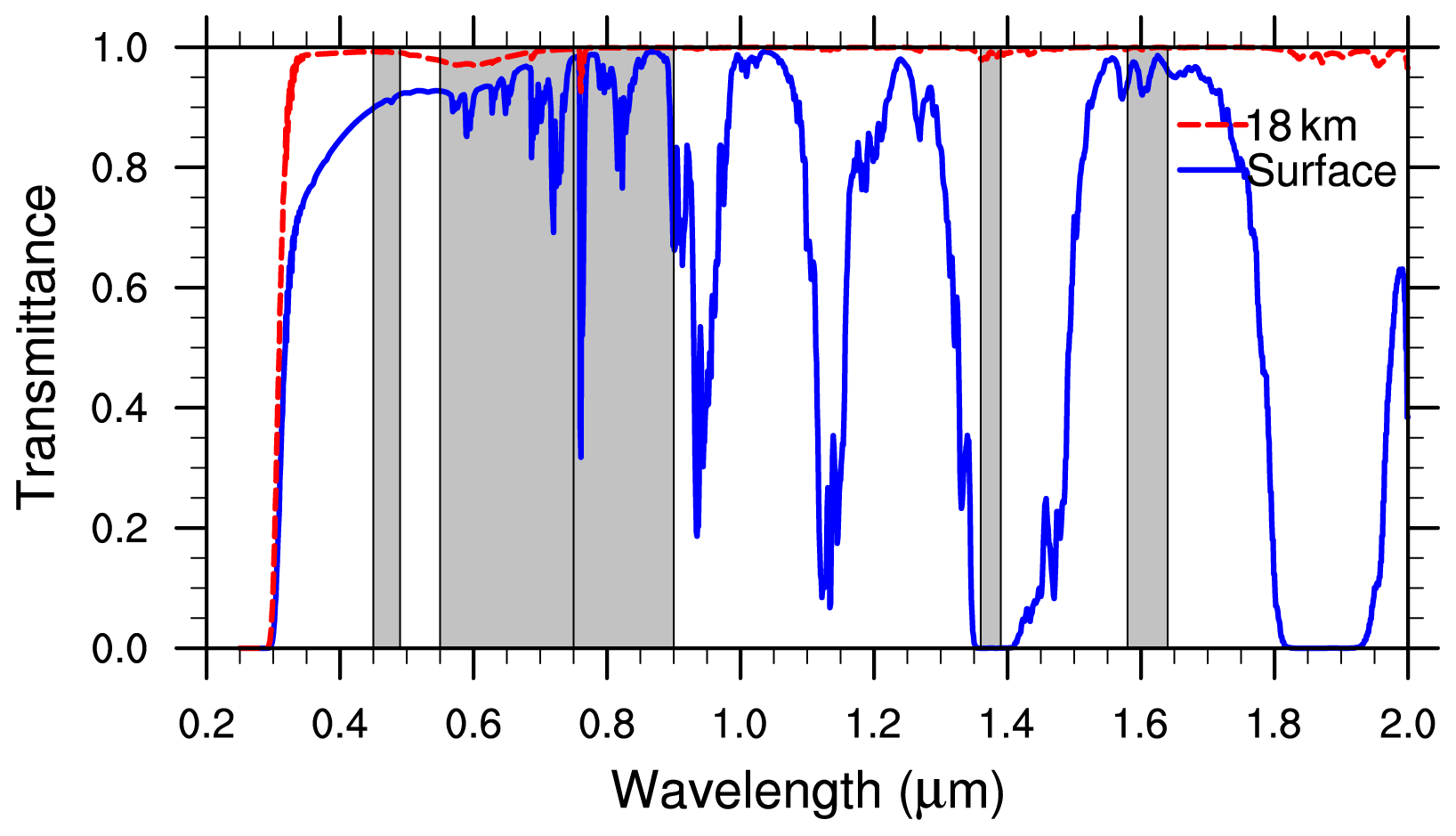
Figure 1Spectral characteristics of FY-4 AGRI bands centered at 0.47, 0.65, 0.825, 1.375, and 1.61 µm. The atmospheric transmittance is calculated for the midlatitude summer temperature and humidity profiles at a solar zenith angle of 10∘.
The introduction of the near-infrared band makes it possible to retrieve Re using FY-4 AGRI. Figure 1 shows the shortwave spectral characteristics of AGRI bands (<2 µm) in the water vapor window. We used the 0.65 and 1.61 µm channels to establish a bispectral lookup table to retrieve the cloud optical thickness (τ) and Re. Both channels have a signal-to-noise ratio >200. We selected FY-4 AGRI Chinese regional scan data from 29 to 30 June 2018. Central and eastern China experienced heavy rain during the Meiyu period at this time and the Integrative Monsoon Frontal Rainfall Experiment was underway. Figure 2 shows an example of 0.65 µm (Fig. 2a), 1.61 µm (Fig. 2b), and 10.8 µm (Fig. 2c) channels of the AGRI and the three important parameters, including the solar zenith angle (Fig. 2d), the viewing zenith angle (Fig. 2e), and the relative azimuth (Fig. 2f). These six parameters were used for the retrieval of the Re profiles.
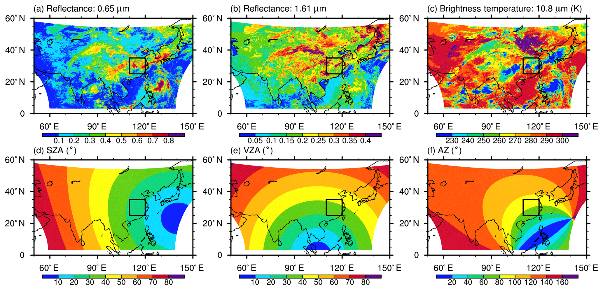
Figure 2Chinese regional scans and geolocation results of FY-4 AGRI at 02:38 UTC on 30 June 2018. (a) Reflectance at 0.65 µm; (b) reflectance at 1.61 µm; (c) brightness temperature at 10.8 µm; (d) solar zenith angle (SZA); (e) viewing zenith angle (VZA); and (f) relative azimuth (AZ). The domain shown in Fig. 4 is indicated.
2.2 Methods
2.2.1 Re retrieval
The spectral Re retrieval algorithms, in which the bispectral reflectance algorithm is the most representative, are based on the optical characteristics of the cloud itself. It was first proposed by Twomey and Seton (1980) to calculate τ and Re. Subsequently, Nakajima and King (1990) extended the scope of the retrieval algorithm and constructed a lookup table, which is currently the official algorithm for MODIS cloud properties. The basic principles of the retrieval algorithm are that the absorption of the cloud droplets is negligible in the visible band and the reflectance mainly depends on the value of τ. In the near-infrared band, the reflection function mainly depends on the cloud particle radius: the smaller the radius, the greater the reflection function. This allows for the simultaneous retrieval of τ and Re. This method has been widely used for the retrieval of cloud properties from multiple onboard instruments (Kawamoto and Nakajima, 2001; Fu, 2014; Letu et al., 2019).
We used the libRadtran library to construct a lookup table for the retrieval of cloud properties. libRadtran is a collection of C and Fortran functions and programs used to calculate solar and thermal radiation in the Earth's atmosphere (Mayer and Kylling, 2005; Emde et al., 2016). Specifically, the atmospheric molecular parameterization scheme selects the LOWTRAN scheme. For water clouds, we select the Mie scheme, which reads in precalculated Mie tables (http://www.libradtran.org, last access: 28 January 2020). Single scattering properties of ice clouds are obtained from Yang et al. (2013) using the severely roughened aggregated column ice crystal habit. The atmospheric temperature and humidity profiles are the preset midlatitude summer profiles. Considering that we are mainly concerned with cloud cluster and precipitation, in order to simplify the model and speed up the calculation, we closed the aerosol module. The setting of the surface type affects the surface albedo. We currently only set two types of underlying surfaces: mixed_forest and ocean_water. The model simulation takes full account of the spectral response functions of the FY-4 AGRI 0.65 and 1.61 µm channels.
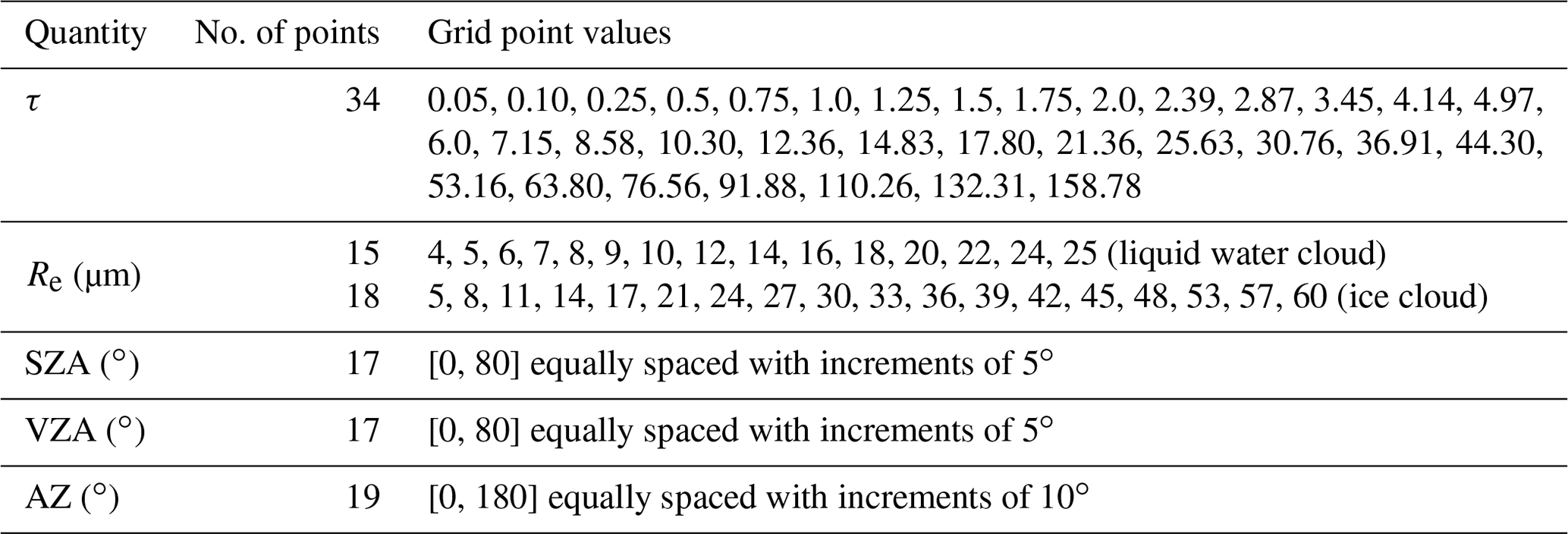
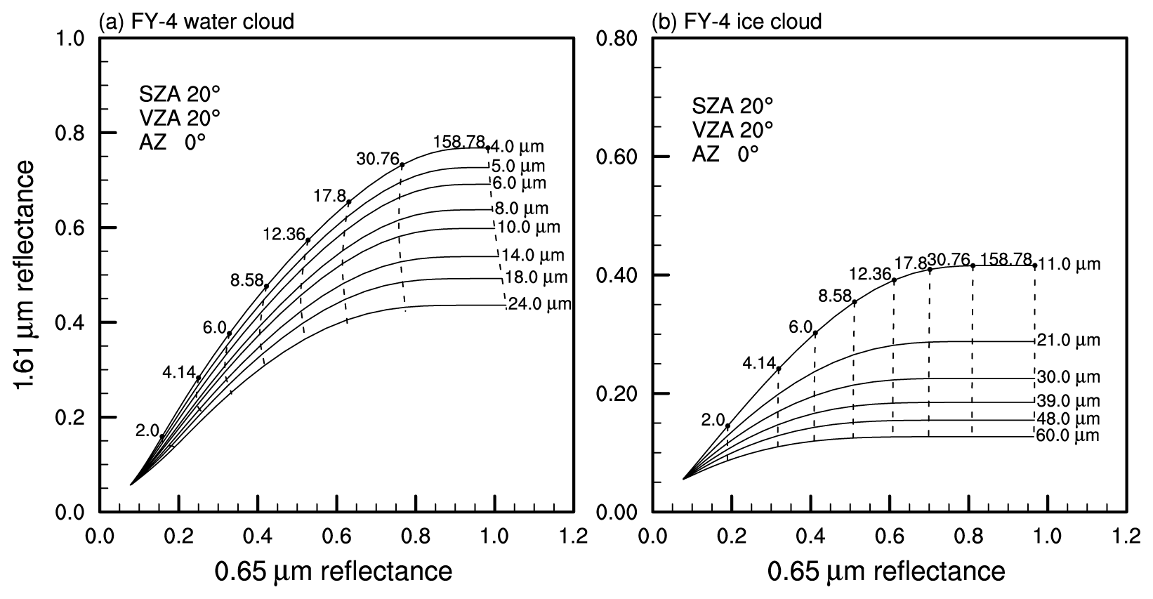
Figure 3Bispectral reflectance lookup table for FY-4 AGRI. Here, solar zenith angle = 20∘, viewing zenith angle = 20∘, relative azimuth = 0∘, and underlying surface = ocean_water.
The lookup table is as a function of τ, Re, solar zenith angle (SZA), viewing zenith angle (VZA), and the relative azimuth (AZ) between the sun and the satellite. Table 1 summarizes the range and grid points for τ, Re, SZA, VZA, and AZ used in constructing lookup tables. Figure 3 shows an example of τ and Re over ocean_water underlying surface for water cloud and ice cloud. The dashed lines represent reflectance contours for fixed τ, and the solid lines are for fixed Re. Since ice and liquid-phase clouds have different scattering properties, it is critical to classify the cloud thermodynamic phase in the retrieval process. It is generally believed that pixels with brightness temperatures lower than 233 K are covered by ice clouds, and temperatures greater than 273 K are covered by water clouds (Menzel and Strabala, 1997), and therefore the thresholds for pure ice cloud and pure water cloud is 233 and 273 K, respectively. When the brightness temperature is between 233 and 273 K, we bring the reflectance into the water-cloud and ice-cloud lookup table simultaneously. As shown in Fig. 3, some combinations of reflectance are definitely ice clouds (or water clouds), and they are treated as pure ice clouds (or water clouds), using the corresponding retrieval lookup table. Otherwise, the differences between the brightness temperature and 233 K (and 273 K) are used as the weights, multiplied by the retrieval values from the water-cloud (and ice-cloud) lookup table, and then we divide the sum of the two by 40 to obtain the cloud parameters of the mixed-cloud pixel. Considering the fact that the thermal infrared channel providing key phase information has a resolution of 4 km (much coarser than MODIS of 1 km), there may be many possibilities such as pure-water cloud, pure-ice cloud, mixed-phase cloud, multilayer cloud, or broken cloud in the pixel. Please note that with the current algorithm it is difficult to handle multilayer cloud and broken cloud. The 1.61 µm channel is also affected by factors such as water vapor and CO2; that is, cloud height may be sensitive to 1.61 µm reflectance. Through conducting the radiative transfer calculations under the most extreme conditions, we found that the impact of cloud height difference in reflectance would not exceed 8 % (figure omitted).
2.2.2 Cloud-cluster identification
The occurrence, development, and dissipation of cloud clusters results in changes in their location, area, cloud-top temperature, average temperature, and precipitation. The process of these changes is relatively continuous (Zhang and Fu, 2018) and continuous pixels with a certain feature are often used to identify a “cloud cluster” or convective system (Mapes and Houze, 1993; Zuidema, 2003; Chen et al., 2017; Chen and Fu, 2017; Huang et al., 2017). For example, Williams and Houze (1987) only considered continuous areas in which the brightness temperature was <213 K when identifying and tracking cloud clusters. However, this algorithm is not suitable for the calculation of the vertical profile of Re, because it only calculates the core area of the convective cloud and ignores the vast areas of low clouds. It therefore cannot obtain a complete Re profile in the vertical direction. If a higher brightness temperature threshold (e.g., 285 K) is used, it is possible to identify a cloud belt that is thousands of kilometers long (such as the Meiyu front system in China). It is not appropriate to treat such a large system as one cloud cluster.
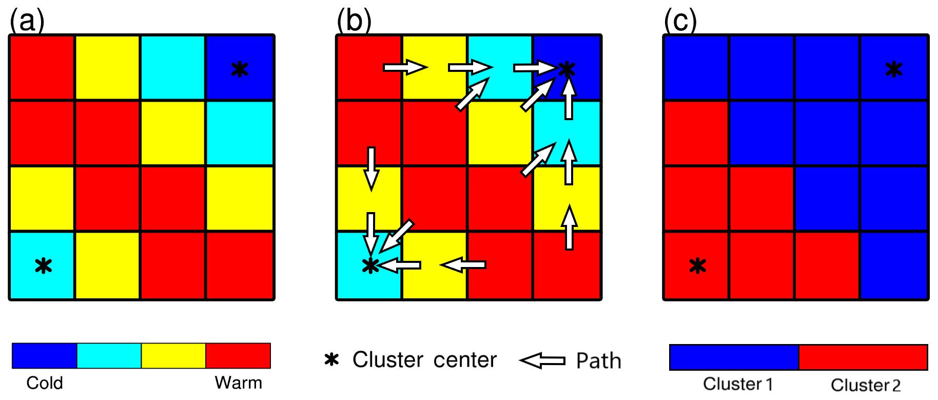
Figure 4Schematic diagram for the maximum temperature gradient method; (a) distribution of the brightness temperature; (b) maximum brightness temperature gradient path of each cloud pixel; (c) the objective cloud-cluster identification product. Please note that the local temperature minimums (asterisks) in the figure are only used to illustrate the maximum temperature gradient method. In the actual calculation, the distance between the two local temperature minimums is greater than 40 km (∼10 pixels).
The strong convective core of a cloud cluster appears as a low value in the brightness temperature, and the surrounding brightness temperature increases as the distance from the core increases. Using this principle, we took the brightness temperature of the 10.8 µm channel and calculated the maximum gradient direction of the brightness temperature of each pixel. We then searched sequentially along this direction until the local minimum point (the cloud convection core) was reached. If this point was marked, then a number of independent cloud clusters could be identified in a large system. The specific algorithm sequence is as follows.
-
The 10.8 µm channel brightness temperature is preprocessed through a Gaussian filter with a standard deviation of 10 pixels and truncated at 4 times the standard deviation. The cloud is assumed to be inhomogeneous and the AGRI instrument has inherent errors in the observations. This means that the final brightness temperature may change over a short horizontal distance. These changes are not physically identified as independent cloud clusters, but they will affect the stability of the algorithm. Gaussian filtering can smooth out the noise of these local minimums by retaining the cloud convective core.
-
The preprocessed 10.8 µm brightness temperature is used to find the local temperature minimum. The local temperature minimum represents the center of the convective core, although there may be multiple convective cores around the lowest temperature core. These convective cores cannot be considered independent cloud clusters in terms of short distance. Therefore, we first calculate local temperature minimums for the complete scene (the brightness temperature is lower than the surrounding 8 pixels) and then set the distance threshold to 40 km (10 pixels). If the distance between two local minimums is lower than this threshold, they would be regarded as the same cloud cluster.
-
Combining the processed 10.8 µm brightness temperature and the local minimum using the maximum temperature gradient method, a sequential search is carried out to determine the convective core to which each pixel belongs, thereby dividing the cloud clusters (Fig. 4). Specifically, take the upper left cloud pixel of the preprocessed scene as the starting point and calculate the brightness temperature gradient of it and its surrounding cloud pixels. Find the pixel that has the greatest brightness temperature gradient with the starting pixel and consider it as the next starting pixel. Repeat this calculation until the starting point is the local minimum obtained in step 2; then the initial starting point belongs to the cloud cluster where this local minimum is located. After traversing all the cloud pixels as starting pixel in the scene, each cloud pixel can belong to a specific local minimum, thus an objective cloud-cluster identification product can be obtained.
The scatter distribution of Re and temperature can be obtained by pairing the retrieved Re of each pixel in the cloud cluster with the 10.8 µm brightness temperature of the pixel itself. Re is sorted by the brightness temperature, and the median and other percentiles of Re are calculated every 2.5 K. To eliminate the errors caused by extreme values, a sorting calculation is only performed in temperature intervals with >30 samples. This allows us to obtain the Re profile of the cloud cluster.
The Meiyu is a persistent, almost stationary precipitation process in the Yangtze River basin in early summer, and it can account for almost half of the annual precipitation in this region. The cloud system along the Meiyu front usually appears as a cloud belt with a latitudinal distribution of thousands of kilometers. It is distributed in the Sichuan Basin through the middle and lower reaches of the Yangtze River to Japan or the western Pacific Ocean. An intensive field campaign (the Integrative Monsoon Frontal Rainfall Experiment) was conducted from June to July 2018 to determine the nature of the Meiyu frontal system through satellite observations, aircraft observations, and model simulations. However, the Meiyu period was short, the precipitation was weak, the rain belt was unstable, and only three Meiyu precipitation processes occurred in 2018 (atypical Meiyu year). According to the assumption of the Re-profile retrieval, wide temperature distribution is beneficial to gain a complete Re profile, and therefore we selected a heavy precipitation event in the experiment to illustrate this retrieval algorithm.

Figure 5Comparison of the pixel-level retrieval of cloud properties using the FY-4 AGRI with Terra MODIS cloud products (Cloud_Optical_Thickness_16 and Cloud_Effective_Radius_16). The observation time of the FY-4 AGRI is 02:38 UTC on 30 June 2018 and the MODIS observation time is 02:55 UTC. The solid lines are provincial boundaries.
Figure 5 shows that the value of τ retrieved by Terra MODIS (Cloud_Optical_Thickness_16) and the FY-4 AGRI has a good spatial consistency, and there are two large centers of τ at about 30∘ N, 113∘ E and 29∘ N, 119∘ E, where the central value of τ is >40. A cloud band with a moderate value of τ occurs in the north of the two large centers (32–33∘ N) where the value of τ is about 20–40. There are regions of thin cloud and clear sky between these large-τ regions. Numerically, the value of τ retrieved by the FY-4 AGRI is close to the MODIS result when the value of τ is small, and it is about 10 % lower than the MODIS τ when the value is large.
The Re of the two instruments showed a similar spatial distribution. The value of the FY-4 AGRI Re is also close to the MODIS result (Cloud_Effective_Radius_16) when the value is small but different when the value is large. It is about 5 µm lower than the MODIS Re when the value is about 50 µm. The MODIS shows more detail inside the cloud band than the FY-4 AGRI. For example, near 34∘ N, 115∘ E, the MODIS Re shows multiple large-value areas, whereas the AGRI Re is less conclusive in the same area. Similarly, in the discrimination of clear-sky regions, the MODIS shows a more elaborate cloud boundary, and some broken cloud regions are identified in the clear-sky region. This is due to the difference in resolution between the two instruments. The horizontal resolution of MODIS products is 1 km, whereas the horizontal resolution of the AGRI is 4 km, which inevitably leads to a lack of local detail.
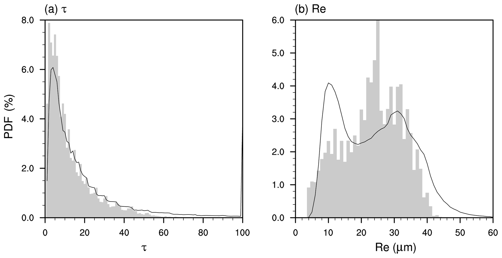
Figure 6Probability density function (PDF) of the FY-4 AGRI retrieval results and the MODIS cloud products in the region shown in Fig. 5. The shaded area shows the FY-4 AGRI results and the solid line is the MODIS results.
Because the pixel position and spatial resolution of the FY-4 AGRI are different from those of the MODIS, the pixel-by-pixel results cannot be compared directly. The probability density function of τ and Re (Fig. 6) in the region shown in Fig. 5 shows similar distribution patterns of the two instruments. The values of τ both show a unimodal distribution with a peak at around 5 and then a rapid decrease. Re appears as a double peak, corresponding to water clouds and ice clouds. Some of the MODIS Re values are >40 µm (accumulated probability <10 %), and the FY-4 AGRI observations do not retrieve these large particles. The MODIS results for τ are slightly greater than the FY-4 AGRI results.
The difference shown in Fig. 6 is most likely due to the partial filling effect caused by different resolutions. Chen and Fu (2017) matched the high-resolution visible pixel (∼ 2 km) to the low-resolution precipitation radar pixel (∼ 5 km) aboard the Tropical Rainfall Measuring Mission satellite, and they found that part of the area in the precipitation pixel measured by the radar was actually clear sky. This interpretation can also be used to explain Fig. 6. We suspect that isolated cirrus clouds with a large Re value, low clouds with a small Re value, and clear skies co-exist in the 4 km region (the FY-4 AGRI pixel resolution) due to the horizontal inhomogeneity of the clouds (e.g., 34.5∘ N, 115∘ E and 34∘ N, 112∘ E in Fig. 5), which means that the FY-4 AGRI only retrieves cloud properties from the overall reflectance, whereas the MODIS can obtain more detailed results. Ackerman et al. (2008) reported that the resolution has a significant impact on cloud observations and care should be taken when comparing results at different resolutions.
The different sensor zenith angles of the two instruments leads to different scattering angles, which have a large effect on the retrieval of the ice-cloud Re. Optically thin cirrus clouds (τ<0.3) and the transition zones between cirrus clouds and clear skies are widely distributed in the tropics and subtropics, and they are difficult to observe with passive optical instruments (Fu et al., 2017). A large sensor zenith angle increases the path length through the upper troposphere, which causes the signals of thin cirrus clouds that are below the limit of resolution to be aggregated (Ackerman et al., 2008). For thin cirrus clouds generated by convective activity, MODIS has a much better detection capability at the edge of the scan than along the center (Maddux et al., 2010). Maddux et al. (2010) used long-term composites to show that, even for the cloud product of MODIS itself, the τ value of the nadir is greater than the τ value of the orbital boundary (∼67∘) by 5–10. The Re value of the ice cloud shows differences of up to 10 µm between the near nadir and near edge of scans over land.
The difference in resolution of the instruments leads to a difference in the retrieval results. The MODIS L3 product releases the cloud properties on a 1∘ grid. To make the retrieval results comparable, we gridded the FY-4 AGRI retrievals to this resolution in the region shown in Fig. 5. In the process of gridding, Re was taken as the arithmetic mean of all the cloud pixels in the grid. In view of the physical meaning of τ itself, direct arithmetic averaging without considering the pattern of distribution within the grid produced a maximum error of 20 % (Chen et al., 2019). We therefore used the logarithmic mean to average τ to a 1∘ grid. Figure 7 shows that, regardless of the value of τ or Re, the results showed a good correlation at a 1∘ grid point. The correlation coefficient of τ reached 0.959, and the correlation coefficient of Re reached 0.933.
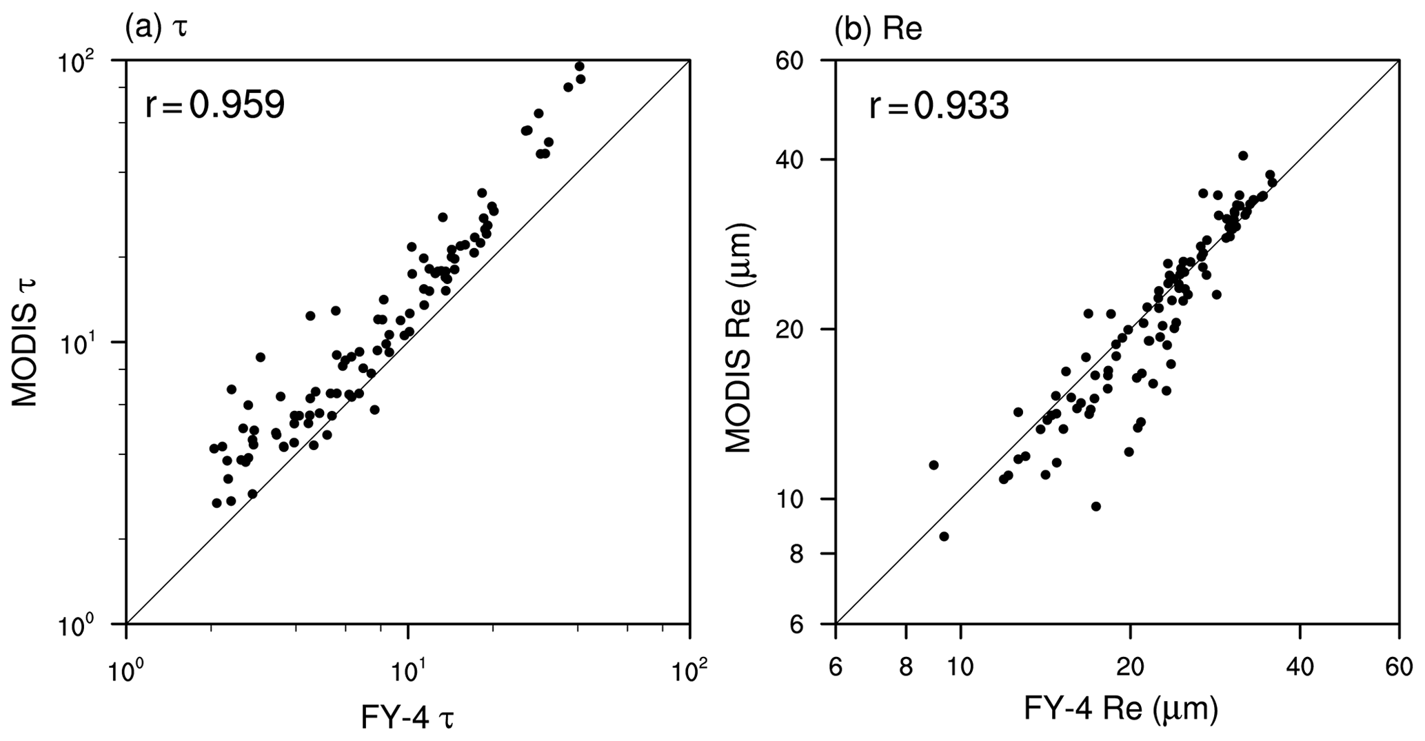
Figure 7Scatter plots of FY-4 AGRI and MODIS retrievals after averaging to a 1∘ grid in the region shown in Fig. 5.

Figure 8Cloud-cluster identification and the corresponding Re profile for the FY-4 AGRI observations in Fig. 5 at 02:38 UTC on 30 June 2018. (a) 10.8 µm brightness temperature; (b) cloud-cluster identification; (c) a specific cloud cluster identified by our algorithm with a base map of Re; and (d) Re profile of the specific cloud cluster.
The retrieval of cloud properties based on FY-4 AGRI was carried out successfully. Figure 8 shows the clustering result from the maximum temperature gradient method. As described in Sect. 2.2.2, Gaussian filtering was performed on the 10.8 µm brightness temperature before clustering, which filtered out broken clouds. The area seen as clear sky in Fig. 8b (white) is therefore greater than that in Fig. 5. The 10.8 µm brightness temperature (Fig. 8a) shows that there is a convective center consisting of three relatively close convective cells near 30∘ N, 113∘ E and the minimum brightness temperature is <200 K. The convective center extends to the southwest as a slender cloud band, which is consistent with the conveyor belt of water vapor during the Meiyu season. The eastern side of the convective center shows another distinct mesoscale convective system with a center at 29∘ N, 119.5∘ E and a minimum brightness temperature of about 210 K. There is a cloud band with a brightness temperature ranging from 220 to 260 K in the north of the two main convective clouds. There are many small-scale clouds in the north of this cloud belt.
The results of automatic clustering are consistent with subjective cognition, showing two main convective cloud clusters and several small cloud clusters on the north side. Our focus is on the convective cloud cluster on the southwest of the area (the purple cloud cluster in Fig. 8b), which produced the heaviest precipitation in the Integrative Monsoon Frontal Rainfall Experiment. The lightning generated by this cloud even destroyed some ground-based instruments. The Re profile is shown in Fig. 8d, where each red dot corresponds to the pixel-by-pixel retrieval of Re in the cloud cluster, and the black line is the median value of Re.
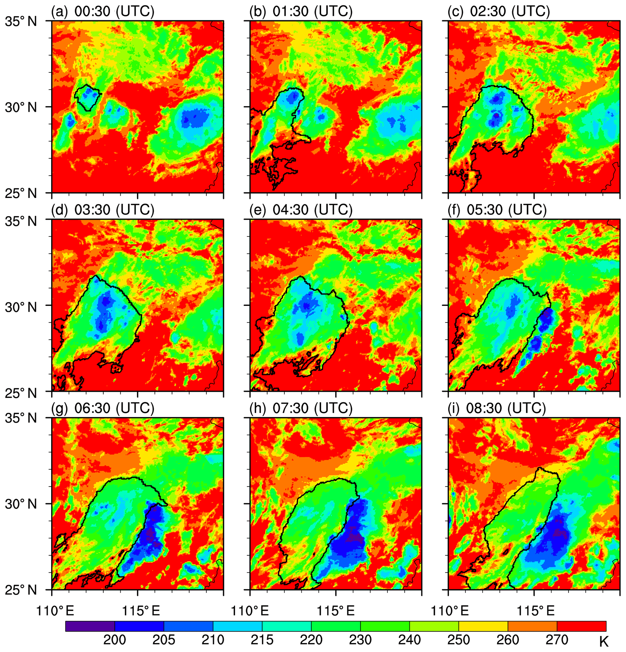
Figure 9Cloud-cluster tracking on 30 June 2018 (1 h intervals). The black line is the continuous cloud cluster identified by the maximum temperature gradient method.
Geostationary satellites enable the continuous observation of the same area, which helps to identify and track the occurrence, development, and dissipation of cloud clusters. Zhang and Fu (2018) proposed that the life stage of clouds affects the convection ratio, the precipitation area, the vertical structure, and the characteristics of precipitation droplets. Using the FY-4 AGRI observations, we achieved the objective segmentation of the cloud, and we brought the segmentation result (cloud cluster) into continuous observations to automatically track the cloud clusters. Figure 9 tracks the purple cloud cluster shown in Fig. 7.
From the perspective of the brightness temperature, there were three adjacent cells with a low temperature on the west side at 00:30 UTC and a large low-temperature zone on the east side. The pattern of cells was irregular, and they were randomly embedded in cloud bands (initiation). By 03:30 UTC, the three cells on the west side had merged to form one cloud cluster (black line), whereas the convective clouds on the east side had gradually dissipated. The convective core appeared to be a linear shape, accompanied with a large area of southwestern-trailing cloud (mature). At 05:30 UTC, the cloud cluster on the west side had started to dissipate, and a slender arcus cloud developed on the eastern boundary with a minimum brightness temperature <200 K. The heavy precipitation of the cloud cluster on the west side (black line) may have caused a local downburst. These cold airflows sink to the ground and flow out to the boundary of the cloud, forming a localized area of ascent with the strong solar heating in the afternoon (∼13:30 LT). This closed circulation created a new, strongly convective cloud at the original cloud boundary. The original convective cloud cluster dissipated, and the newly formed convective cloud cluster on the east side gradually developed and matured. From the perspective of the tracked cloud (black line), our objective tracking results successfully described the development and dissipation of this cloud cluster without confusing it with the newly generated convective cloud cluster in the east.

Figure 10Changes in the Re profile (25, 50, and 75 percentiles) in the tracked continuous cloud cluster at 1 h intervals. Horizontal dashed lines represent temperatures of 273 and 233 K, respectively. The text in the figure gives the area of the cloud cluster and the coldest 10 % brightness temperature (BT) of the cluster.
Figure 10 shows the evolution of the Re vertical profile for the automatically tracked cloud cluster. In terms of the area of the cluster, the rapid growth and development period of the cloud cluster was from 00:30 to 02:30 UTC. The cloud cluster area was relatively stable from 02:30 to 06:30 UTC, after which time the area was slightly decreased. In agreement with the theory of Rosenfeld and Lensky (1998), the change in Re with temperature can be divided into five distinct zones: the diffusional droplet growth zone, the droplet coalescence growth zone, the rainout zone, the mixed-phase zone, and the glaciated zone. These five areas do not all necessarily appear in a given cloud cluster.
Only the small convective cell was identified at 00:30 UTC, and it did not contain enough pixels with high temperature (<30 samples in 2.5 K temperature interval). Although there must be a region for particles to condense and coalesce within this cloud cluster, due to technical limitations, only the glaciated zone was shown in the Re profile (Fig. 10a). At 01:30 UTC, convective cells merged and the convection activity was strong. The Re profile showed that in areas where the temperature was <230 K, Re was stable in the glaciated zone from 28 to 32 µm. Re changed almost linearly with temperature between 285 and 230 K, and it did not exhibit a clear boundary between the diffusional growth zone, the coalescence growth zone, the rainout zone, or the mixed-phase zone. This is because a strong convective core usually has a strong ascending motion. Under the influence of such strong ascending motion, the boundary between the zones is broken and there is not enough time for the growth of precipitation (Fig. 10b). Rosenfeld et al. (2008) explained that this situation may delay the development of both the mixed and ice phases at higher altitudes and that the resulting linear Re profile is a warning of severe weather.
The Re profile gradually showed multiple zones from 02:30 to 03:30 UTC, and the multiple zones are most distinct from 04:30 to 05:30 UTC. The median Re slowly increased with temperature from 10 to 16 µm (∼285 to 270 K), which is the growth zone in which cloud droplets are mainly condensed and affected by the number of CCN. The growth rate of Re accelerated significantly from 16 to 22 µm (∼270 to 265 K). At this time, raindrops were formed and the growth of cloud droplets mainly depended on coalescence. The distinct zones can also be seen in the 25th and 75th percentiles, while the turning points of Re and the growth rates differ from the median. A possible explanation is that turning points and growth rates are affected not only by temperature but also by the size of Re. The rainout zone usually appears in marine cloud systems with fewer CCN (Martins et al., 2011), whereas this precipitation process was located in inland China. A large number of artificial aerosols act as CCN to suppress warm rain while delaying freezing, which requires lower temperatures. From ∼265 to ∼230 K, the rate of increase in Re slightly slows down. The cloud particles gradually change from the liquid phase to the ice phase, and their radius increases and absorbs more near-infrared radiation (mixed-phase zone). Re remains stable below 230 K and the profile is completely in the glaciated zone. After 06:30 UTC, the intensity of the original cloud cluster was significantly weakened and gradually dissipated. The Re profile gradually became difficult to describe. This is due to the weakening of convective activity, and the cloud cluster is mainly governed by a thinning anvil. Affected by the low-level clouds and high-level anvils, the uncertainty of the Re retrieval increases, and the brightness temperature cannot represent the cloud-top temperature at this time, which reduces the credibility of the Re profile.
FY-4A is the first Chinese next-generation geostationary meteorological satellite. It was launched in 2016 and began operation in 2018. Here, the bispectral reflectance algorithm was used to retrieve Re and τ. We used the maximum temperature gradient method to automatically segment, identify, and track cloud clusters. We obtained the objective cloud cluster Re profile retrieval method based on FY-4 AGRI observations by combining these two methods. Taking a severe weather event during the Integrative Monsoon Frontal Rainfall Experiment campaign as an example, we calculated the Re profiles of an objective cloud cluster at different life stages.
The cloud properties of Re and τ retrieved from the FY-4 AGRI were compared with the Terra MODIS cloud products. The results showed that they were in good agreement with the spatial distribution, although there were some differences when the value was large, which may be due to the difference in resolution and the viewing zenith angles. The results showed a strong correlation when the FY-4 AGRI and MODIS retrievals were both averaged to a 1∘ grid. This indicates that the cloud properties retrieved by the FY-4 AGRI were credible.
The maximum temperature gradient method effectively divides thousands of kilometers of cloud bands into multiple cloud clusters, and the objective results are consistent with subjective cognition. For this specific severe weather event, the method tracked the complete process of development, maturation, and dissipation of a convective cloud cluster. The Re profiles of the cloud cluster showed completely different characteristics at different life stages. During the development stage, Re changed almost linearly with temperature, whereas during the mature stage the Re profile showed multiple zones of changes with temperature. Different Re profiles reflected the different physical processes of cloud particle growth and corresponded to completely different processes of formation of precipitation.
The use of geostationary satellites to obtain continuous cloud-cluster Re vertical profiles has led to many different applications. For example, the Re profile of the development stage is linear, which may help to improve the predictive skill for the nowcasting of storms. Real-time changes in the shape of the Re profile may also be used to characterize the life stages of clouds. The position of the glaciation temperature and the mixed-phase zone in the Re profile indicates the formation of mixed-layer precipitation. The continuous change in the glaciation temperature helps our understanding of mixed-layer precipitation. We are confident that the introduction of the cloud-cluster Re profile will help to improve the future application of FY-4 data in meteorology.
Data supporting this paper can be found at http://fy4.nsmc.org.cn/data/en/code/FY4A.html#AGRI (last access: 28 January 2020) (Yang et al., 2017).
YC conceptualized this research and wrote the paper. YC, GC, and AZ designed the algorithms, performed the simulations, and analyzed the results. CC, RW, SZ, DW, and YF validated, discussed, and edited the paper. YF supervised the research.
The authors declare that they have no conflict of interest.
This work is supported by the National Natural Science Foundation of China (grant 91837310, 41675041, 41620104009), the National Key Research and Development Program of China (grant nos. 2017YFC1501402 and 2018YFC1507200), and the Key research and development projects in Anhui province (201904a07020099).
This research has been supported by the National Natural Science Foundation of China (grant nos. 91837310, 41675041, 41620104009), the National Key Research and Development Program of China (grant nos. 2017YFC1501402 and 2018YFC1507200), and the Key research and development projects in Anhui province (grant no. 201904a07020099).
This paper was edited by Johannes Quaas and reviewed by two anonymous referees.
Ackerman, S. A., Holz, R. E., Frey, R., Eloranta, E. W., Maddux, B. C., and Mcgill, M.: Cloud detection with MODIS. Part II: Validation, J. Atmos. Ocean. Tech., 25, 1073–1086, https://doi.org/10.1175/2007JTECHA1053.1, 2008.
Andreae, M. O., Rosenfeld, D., Artaxo, P., Costa, A. A., Frank, G. P., Longo, K. M., and Silva-Dias, M. A. F.: Smoking rain clouds over the Amazon, Science, 303, 1337–1342, https://doi.org/10.1126/science.1092779, 2004.
Ansmann, A., Tesche, M., Althausen, D., Müller, D., Seifert, P., Freudenthaler, V., Heese, B., Wiegner, M., Pisani, G., Knippertz, P., and Dubovik, O.: Influence of Saharan dust on cloud glaciation in southern Morocco during the Saharan Mineral Dust Experiment, J. Geophys. Res., 113, D04210, https://doi.org/10.1029/2007JD008785, 2008.
Braga, R. C., Rosenfeld, D., Weigel, R., Jurkat, T., Andreae, M. O., Wendisch, M., Pöschl, U., Voigt, C., Mahnke, C., Borrmann, S., Albrecht, R. I., Molleker, S., Vila, D. A., Machado, L. A. T., and Grulich, L.: Further evidence for CCN aerosol concentrations determining the height of warm rain and ice initiation in convective clouds over the Amazon basin, Atmos. Chem. Phys., 17, 14433–14456, https://doi.org/10.5194/acp-17-14433-2017, 2017.
Chang, F. and Li, Z.: Estimating the vertical variation of cloud droplet effective radius using multispectral near-infrared satellite measurements, J. Geophys. Res., 107, 7-1–7-12, https://doi.org/10.1029/2001JD000766, 2002.
Chang, F. and Li, Z.: Retrieving vertical profiles of water-cloud droplet effective radius: Algorithm modification and preliminary application, J. Geophys. Res.-Atmos., 108, 4763–4773, https://doi.org/10.1029/2003JD003906, 2003.
Chen, Y. and Fu, Y.: Characteristics of VIRS Signals within Pixels of TRMM PR for Warm Rain in the Tropics and Subtropics, J. Appl. Meteorol. Clim., 56, 789–801, https://doi.org/10.1175/JAMC-D-16-0198.1, 2017.
Chen, Y., Fu, Y., Xian, T., and Pan, X.: Characteristics of cloud cluster over the steep southern slopes of the Himalayas observed by CloudSat, Int. J. Climatol., 37, 4043–4052, https://doi.org/10.1002/joc.4992, 2017.
Chen, Y., Chong, K., and Fu, Y.: Impacts of distribution patterns of cloud optical depth on the calculation of radiative forcing, Atmos. Res., 218, 70–77, https://doi.org/10.1016/j.atmosres.2018.11.007, 2019.
Delanoe, J. and Hogan, R. J.: Combined CloudSat-CALIPSO-MODIS retrievals of the properties of ice clouds, J. Geophys. Res., 115, D00H29, https://doi.org/10.1029/2009JD012346, 2010.
Deng, M., Mace, G. G., Wang, Z., and Paul Lawson, R.: Evaluation of Several A-Train Ice Cloud Retrieval Products with In Situ Measurements Collected during the SPARTICUS Campaign, J. Appl. Meteor. Climatol., 52, 1014–1030, https://doi.org/10.1175/JAMC-D-12-054.1, 2013.
Emde, C., Buras-Schnell, R., Kylling, A., Mayer, B., Gasteiger, J., Hamann, U., Kylling, J., Richter, B., Pause, C., Dowling, T., and Bugliaro, L.: The libRadtran software package for radiative transfer calculations (version 2.0.1), Geosci. Model Dev., 9, 1647–1672, https://doi.org/10.5194/gmd-9-1647-2016, 2016.
Ewald, F., Zinner, T., Kölling, T., and Mayer, B.: Remote sensing of cloud droplet radius profiles using solar reflectance from cloud sides – Part 1: Retrieval development and characterization, Atmos. Meas. Tech., 12, 1183–1206, https://doi.org/10.5194/amt-12-1183-2019, 2019.
Freud, E. and Rosenfeld, D.: Linear relation between convective cloud drop number concentration and depth for rain initiation, J. Geophys. Res.-Atmos., 117, D02207, https://doi.org/10.1029/2011JD016457, 2012.
Fu, Y.: Cloud parameters retrieved by the bispectral reflectance algorithm and associated applications, J. Meteorol. Res., 28, 965–982, https://doi.org/10.1007/s13351-014-3292-3, 2014.
Fu, Y., Chen, Y., Li, R., Qin, F., Xian, T., Yu, L., Zhang, A., Liu, G., and Zhang, X.: Lateral Boundary of Cirrus Cloud from CALIPSO Observations, Sci. Rep.-UK, 7, 14221, https://doi.org/10.1038/s41598-017-14665-6, 2017.
Huang, Y., Meng, Z., Li, J., Li, W., Bai, L., Zhang, M., and Wang, X.: Distribution and variability of satellite-derived signals of isolated convection initiation events over central eastern China, J. Geophys. Res.-Atmos., 122, 11357–11373, https://doi.org/10.1002/2017JD026946, 2017.
Kawamoto, K. and Nakajima, T.: A global determination of cloud microphysics with AVHRR remote sensing, J. Climate, 14, 2054–2068, https://doi.org/10.1175/1520-0442(2001)014<2054:AGDOCM>2.0.CO;2, 2001.
King, N. J. and Vaughan, G.: Using passive remote sensing to retrieve the vertical variation of cloud droplet size in marine stratocumulus: An assessment of information content and the potential for improved retrievals from hyperspectral measurements, J. Geophys. Res.-Atmos., 117, D15206, https://doi.org/10.1029/2012JD017896, 2012.
Lensky, I. M. and Rosenfeld, D.: The time-space exchangeability of satellite retrieved relations between cloud top temperature and particle effective radius, Atmos. Chem. Phys., 6, 2887–2894, https://doi.org/10.5194/acp-6-2887-2006, 2006.
Letu, H., Nagao, T. M, Nakajima, T. Y., Riedi, J., Ishimoto, H., Baran, A. J., Shang, H., Sekiguchi, M., and Kikuchi, M.: Ice cloud properties from Himawari-8/AHI next-generation geostationary satellite: capability of the AHI to monitor the dc cloud generation process, IEEE T. Geosci. Remote, 57, 3229–3239, https://doi.org/10.1109/TGRS.2018.2882803, 2019.
Liou, K. N.: Influence of cirrus clouds on weather and climate processes: a global perspective, Mon. Weather Rev., 114, 1167–1199, 1986.
Maddux, B. C., Ackerman, S. A., and Platnick, S.: Viewing Geometry Dependencies in MODIS Cloud Products, J. Atmos. Ocean. Tech., 27, 1519–1528, https://doi.org/10.1175/2010JTECHA1432.1, 2010.
Mapes, B. E. and Houze, R. A.: Cloud clusters and superclusters over the oceanic warm pool, Mon. Weather Rev., 121, 1398–1415, 1993.
Martins, J. V., Marshak, A., Remer, L. A., Rosenfeld, D., Kaufman, Y. J., Fernandez-Borda, R., Koren, I., Correia, A. L., Zubko, V., and Artaxo, P.: Remote sensing the vertical profile of cloud droplet effective radius, thermodynamic phase, and temperature, Atmos. Chem. Phys., 11, 9485–9501, https://doi.org/10.5194/acp-11-9485-2011, 2011.
Mayer, B. and Kylling, A.: Technical note: The libRadtran software package for radiative transfer calculations – description and examples of use, Atmos. Chem. Phys., 5, 1855–1877, https://doi.org/10.5194/acp-5-1855-2005, 2005.
Menzel, P. and Strabala K.: Cloud top properties and cloud phase algorithm theoretical basis document, University of Wisconsin-Madison, Madison, USA, 1997.
Min, M., Wu, C., Li, C., Liu, H., Xu, N., Wu, X., Chen, L., Wang, F., Sun, F., Qin, D., Wang, X., Li, B., Zheng, Z., Cao, G., and Dong, L.: Developing the Science Product Algorithm Testbed for Chinese Next-Generation Geostationary Meteorological Satellites: Fengyun-4 Series, J. Meteorol. Res.-Prc., 31, 708–719, https://doi.org/10.1007/s13351-017-6161-z, 2017.
Nakajima, T. and King, M. D.: Determination of the optical-thickness and effective particle radius of clouds from reflected solar-radiation measurements. 1. Theory, J. Atmos. Sci., 47, 1878–1893, https://doi.org/10.1175/1520-0469(1990)047<1878:DOTOTA>2.0.CO;2, 1990.
Oki, T. and Kanae, S.: Global hydrological cycles and world water resources, Science, 313, 1068–1072, https://doi.org/10.1126/science.1128845, 2006.
Painemal, D. and Zuidema, P.: Assessment of MODIS cloud effective radius and optical thickness retrievals over the Southeast Pacific with VOCALS-REx in situ measurements, J. Geophys. Res.-Atmos., 116, D24206, https://doi.org/10.1029/2011JD016155, 2011.
Pawlowska, H., Brenguier, J. L., and Burnet, F.: Microphysical properties of stratocumulus clouds, Atmos. Res., 55, 15–33, https://doi.org/10.1016/S0169-8095(00)00054-5, 2000.
Platnick, S.: Vertical photon transport in cloud remote sensing problems, J. Geophys. Res.-Atmos., 105, 22919–22935, https://doi.org/10.1029/2000JD900333, 2000.
Prabha, T. V., Khain, A., Maheshkumar, R. S., Pandithurai, G., Kulkarni, J. R., Konwar, M., and Goswami, B. N.: Microphysics of premonsoon and monsoon clouds as seen from in situ measurements during the Cloud Aerosol Interaction and Precipitation Enhancement Experiment (CAIPEEX), J. Atmos. Sci., 68, 1882–1901, https://doi.org/10.1175/2011JAS3707.1, 2011.
Rangno, A. L. and Hobbs, P. V.: Microstructures and precipitation development in cumulus and small cumulonimbus clouds over the warm pool of the tropical Pacific Ocean, Q. J. Roy. Meteor. Soc., 131, 639–673, 2005.
Rosenfeld, D.: TRMM observed first direct evidence of smoke from forest fires inhibiting rainfall, Geophys. Res. Lett., 26, 3105–3108, https://doi.org/10.1029/1999GL006066, 1999.
Rosenfeld, D.: Suppression of rain and snow by urban and industrial air pollution, Science, 287, 1793–1796, https://doi.org/10.1126/science.287.5459.1793, 2000.
Rosenfeld, D.: Chapter 6 – Cloud-aerosol-precipitation interactions based of satellite retrieved vertical profiles of cloud microstructure, edited, pp. 129–152, Elsevier Inc, https://doi.org/10.1016/B978-0-12-810437-8.00006-2, 2018.
Rosenfeld, D. and Gutman, G.: Retrieving microphysical properties near the tops of potential rain clouds by multispectral analysis of AVHRR data, Atmos. Res., 34, 259–283, https://doi.org/10.1016/0169-8095(94)90096-5, 1994.
Rosenfeld, D. and Lensky, I. M.: Satellite-based insights into precipitation formation processes in continental and maritime convective clouds, B. Am. Meteorol. Soc., 79, 2457–2476, https://doi.org/10.1175/1520-0477(1998)079<2457:SBIIPF>2.0.CO;2, 1998.
Rosenfeld, D., Yu, X., and Dai, J.: Satellite-retrieved microstructure of AgI seeding tracks in supercooled layer clouds, J. Appl. Meteorol., 44, 760–767, https://doi.org/10.1175/JAM2225.1, 2005.
Rosenfeld, D., Woodley, W. L., Krauss, T. W., and Makitov, V.: Aircraft microphysical documentation from cloud base to anvils of hailstorm feeder clouds in Argentina, J. Appl. Meteorol. Clim., 45, 1261–1281, https://doi.org/10.1175/JAM2403.1, 2006.
Rosenfeld, D., Dai, J., Yu, X., Yao, Z., Xu, X., Yang, X., and Du, C.: Inverse relations between amounts of air pollution and orographic precipitation, Science, 315, 1396–1398, 2007.
Rosenfeld, D., Woodley, W. L., Lerner, A., Kelman, G., and Lindsey, D. T.: Satellite detection of severe convective storms by their retrieved vertical profiles of cloud particle effective radius and thermodynamic phase, J. Geophys. Res., 113, D04208, https://doi.org/10.1029/2007JD008600, 2008.
Rosenfeld, D., Yu, X., Liu, G., Xu, X., Zhu, Y., Yue, Z., Dai, J., Dong, Z., Dong, Y., and Peng, Y.: Glaciation temperatures of convective clouds ingesting desert dust, air pollution and smoke from forest fires, Geophys. Res. Lett., 38, L21804, https://doi.org/10.1029/2011GL049423, 2011.
Rosenfeld, D., Wang, H., and Rasch, P. J.: The roles of cloud drop effective radius and LWP in determining rain properties in marine stratocumulus, Geophys. Res. Lett., 39, L13801, https://doi.org/10.1029/2012GL052028, 2012a.
Rosenfeld, D., Woodley, W. L., Khain, A., Cotton, W. R., Carrió, G., Ginis, I., and Golden, J. H.: Aerosol effects on microstructure and intensity of tropical cyclones, B. Am. Meteorol. Soc., 93, 987–1001, 2012b.
Rossow, W. B. and Schiffer, R. A.: Advances in understanding clouds from ISCCP, B. Am. Meteorol. Soc., 80, 2261–2287, 1999.
Suzuki, K., Nakajima, T. Y., and Stephens, G. L.: Particle growth and drop collection efficiency of warm clouds as inferred from joint CloudSat and MODIS observations, J. Atmos. Sci., 67, 3019–3032, https://doi.org/10.1175/2010JAS3463.1, 2010.
Suzuki, K., Stephens, G. L., Van Den Heever, S. C., and Nakajima, T. Y.: Diagnosis of the warm rain process in cloud-resolving models using joint CloudSat and MODIS observations, J. Atmos. Sci., 68, 2655–2670, https://doi.org/10.1175/JAS-D-10-05026.1, 2011.
Twomey, S. and Seton, K. J.: Inferences of gross microphysical properties of clouds from spectral reflectance measurements, J. Atmos. Sci., 37, 1065–1069, https://doi.org/10.1175/1520-0469(1980)037<1065:IOGMPO>2.0.CO;2, 1980.
Wendisch, M., Poschl, U., Andreae, M. O., MacHado, L. A. T., Albrecht, R., Schlager, H., Rosenfeld, D., Martin, S. T., Abdelmonem, A., Afchine, A., Araujo, A. C., Artaxo, P., Aufmhoff, H., Barbosa, H. M. J., Borrmann, S., Braga, R., Buchholz, B., Cecchini, M. A., Costa, A., Curtius, J., Dollner, M., Dorf, M., Dreiling, V., Ebert, V., Ehrlich, A., Ewald, F., Fisch, G., Fix, A., Frank, F., Futterer, D., Heckl, C., Heidelberg, F., Huneke, T., Jakel, E., Jarvinen, E., Jurkat, T., Kanter, S., Kastner, U., Kenntner, M., Kesselmeier, J., Klimach, T., Knecht, M., Kohl, R., Kolling, T., Kramer, M., Kruger, M., Krisna, T. C., Lavric, J. V., Longo, K., Mahnke, C., Manzi, A. O., Mayer, B., Mertes, S., Minikin, A., Molleker, S., Munch, S., Nillius, B., Pfeilsticker, K., Pohlker, C., Roiger, A., Rose, D., Rosenow, D., Sauer, D., Schnaiter, M., Schneider, J., Schulz, C., De Souza, R. A. F., Spanu, A., Stock, P., Vila, D., Voigt, C., Walser, A., Walter, D., Weigel, R., Weinzierl, B., Werner, F., Yamasoe, M. A., Ziereis, H., Zinner, T., and Zoger, M.: Acridicon–chuva campaign: studying tropical deep convective clouds and precipitation over Amazonia using the new German research aircraft HALO, B. Am. Meteorol. Soc., 97, 1885–1908, https://doi.org/10.1175/BAMS-D-14-00255.1, 2016.
Wetherald, R. T. and Manabe, S.: Cloud feedback processes in a general-circulation model, J. Atmos. Sci., 45, 1397–1415, 1988.
Williams, M. and Houze, R. A.: Satellite-observed characteristics of winter monsoon cloud clusters, Mon. Weather Rev., 115, 505–519, 1987.
Yang, J., Zhang, Z., Wei, C., Lu, F., and Guo, Q.: Introducing the new generation of Chinese geostationary weather satellites, FENGYUN-4, B. Am. Meteorol. Soc., 98, 1637–1658, https://doi.org/10.1175/BAMS-D-16-0065.1, 2017 (data available at: http://fy4.nsmc.org.cn/data/en/code/FY4A.html#AGRI, last access: 28 January 2020).
Yang, P., Bi, L., Baum, B. A., Liou, K. N., and Cole, B.: Spectrally consistent scattering, absorption, and polarization properties of atmospheric ice crystals at wavelengths from 0.2 to 100 µm, J. Atmos. Sci., 70, 330–347, https://doi.org/10.1175/JAS-D-12-039.1, 2013.
Zhang, A. and Fu, Y.: Life cycle effects on the vertical structure of precipitation in east china measured by Himawari-8 and GPM DPR, Mon. Weather Rev., 146, 2183–2199, 2018.
Zheng, Y. and Rosenfeld, D.: Linear relation between convective cloud base height and updrafts and application to satellite retrievals, Geophys. Res. Lett., 42, 6485–6491, https://doi.org/10.1002/2015GL064809, 2015.
Zhu, L., Li, J., Zhao, Y., Gong, H., and Li, W.: Retrieval of volcanic ash height from satellite-based infrared measurements, J. Geophys. Res.-Atmos., 122, 5364–5379, https://doi.org/10.1002/2016JD026263, 2017.
Zuidema, P.: Convective clouds over the Bay of Bengal, Mon. Weather Rev., 131, 780–798, 2003.