the Creative Commons Attribution 4.0 License.
the Creative Commons Attribution 4.0 License.
 | 09 Aug 2019
Role of climate model dynamics in estimated climate responses to anthropogenic aerosols
Hannele Korhonen
Petri Räisänen
Muzaffer Ege Alper
Petteri Uotila
Declan O'Donnell
Joonas Merikanto
Significant discrepancies remain in estimates of climate impacts of anthropogenic aerosols between different general circulation models (GCMs). Here, we demonstrate that eliminating differences in model aerosol or radiative forcing fields results in close agreement in simulated globally averaged temperature and precipitation responses in the studied GCMs. However, it does not erase the differences in regional responses. We carry out experiments of equilibrium climate response to modern-day anthropogenic aerosols using an identical representation of anthropogenic aerosol optical properties and the first indirect effect of aerosols, MACv2-SP (a simple plume implementation of the second version of the Max Planck Institute Aerosol CLimatology), in two independent climate models (NorESM, Norwegian Earth System Model, and ECHAM6). We find consistent global average temperature responses of −0.48 (±0.02) and −0.50 (±0.03) K and precipitation responses of −1.69 (±0.04) % and −1.79 (±0.05) % in NorESM1 and ECHAM6, respectively, compared to modern-day equilibrium climate without anthropogenic aerosols. However, significant differences remain between the two GCMs' regional temperature responses around the Arctic circle and the Equator and precipitation responses in the tropics. The scatter in the simulated globally averaged responses is small in magnitude when compared against literature data from modern GCMs using model intrinsic aerosols but same aerosol emissions −(0.5–1.1) K and −(1.5–3.1) % for temperature and precipitation, respectively). The Pearson correlation of regional temperature (precipitation) response in these literature model experiments with intrinsic aerosols is 0.79 (0.34). The corresponding correlation coefficient for NorESM1 and ECHAM6 runs with identical aerosols is 0.78 (0.41). The lack of improvement in correlation coefficients between models with identical aerosols and models with intrinsic aerosols implies that the spatial distribution of regional climate responses is not improved via homogenizing the aerosol descriptions in the models. Rather, differences in the atmospheric dynamic and snow/sea ice cover responses dominate the differences in regional climate responses. Hence, even if we would have perfect aerosol descriptions inside the global climate models, uncertainty arising from the differences in circulation responses between the models would likely still result in a significant uncertainty in regional climate responses.


Making reliable predictions on future changes in regional climates is crucial for estimating how climate change will impact people and societies (Hawkins et al., 2016), but there are still large uncertainties related to climate change predictions on regional scales (Giorgi and Francisco, 2000; Feser et al., 2011). Anthropogenic aerosol particles can be an important driver for regional climate change due to the near-instantaneous response of local aerosol concentrations to changes in emissions, their direct radiative properties and their ability to modify cloud microphysical processes. However, reliable implementation of aerosol effects into global climate models has been challenging. Several aerosol processes are still not well understood (Boucher et al., 2013), and there exists an enormous scale difference between the microphysical processes and the resolution of global-scale models (Carslaw et al., 2013).
Varying descriptions of aerosols and aerosol–cloud interactions cause a wide spread in aerosol radiative forcing and climate impacts between different general circulation models (GCMs) (Wilcox et al., 2015). Shindell et al. (2015) compared historical Coupled Model Intercomparison Project phase 5 (CMIP5) runs with and without anthropogenic forcing from aerosols, ozone and land use. The forcing showed a very large spatial variation with globally averaged values that ranged between 0.15 and (the aerosol contribution being between −0.29 and ). The combined changes in aerosol, ozone and land use produced globally averaged transient temperature responses between 0.00 and −1.33 K over the 20th century, with the spatial pattern of the temperature response varying significantly between the models. Overall, the inclusion of aerosols in CMIP5 models nevertheless improved the historical temperature trends compared to observations. This applied particularly to models including sophisticated parameterizations for aerosol cloud droplet activation (Ekman, 2014).
Besides reducing the global temperature, anthropogenic aerosols are also known to reduce global precipitation (Ramanathan, 2005) and to significantly modify the Asian monsoon (Bollasina et al., 2011; Salzmann et al., 2014). Wang (2015) demonstrated that among CMIP5 models the changes in anthropogenic aerosols dominated the total precipitation changes from the pre-industrial era to the present day. Most of this change was caused by the remote impact of aerosols rather than by direct effects on local cloud processes and cloud optical depth in all but heavily aerosol-loaded regions, such as in the Indian monsoon region. Also, for precipitation changes, an improved representation of aerosol–cloud interactions was found to be the key factor in reproducing consistent distributions of past precipitation change.
Improvements in model aerosol descriptions have not succeeded to remove the large uncertainty in aerosol climate effects. After CMIP5, the most representative multi-model results on aerosol climate impacts have been provided by Samset et al. (2018). They compared the equilibrium climate responses for complete removals of model intrinsic anthropogenic aerosols among four state-of-the-art fully coupled climate models, with aerosol emissions from CMIP5 (Lamarque et al., 2010). In their study, removing the aerosols produced global-mean temperature increases between 0.5 and 1.1 K and precipitation increases between 1.5 % and 3.1 %. In another recent study, Kasoar et al. (2016) reduced anthropogenic SO2 emissions from China in three independent climate models. There, identical emission reductions lead to simulated changes in aerosol optical depth and shortwave radiative flux over China that varied by up to a factor of 6 between the models. The three models also exhibited large differences in their global and regional temperature responses. However, it is unclear to which degree the existing spread in aerosol climate impacts among current climate models results from differences in modeled aerosols or from differences in model dynamical responses to aerosols. Only standardized aerosol perturbations across different models can entangle these sources of uncertainties in aerosol climate effects (Stier et al., 2013).
Here, we explore how robust the aerosol climate response would be in modern GCMs if the anthropogenic aerosols and their cloud interactions could be modeled exactly. To assess this question, we carry out long equilibrium climate simulations with fixed greenhouse gas concentrations and prescribed aerosol fields using the MACv2-SP (a simple plume implementation of the second version of the Max Planck Institute Aerosol CLimatology) aerosol description (Stevens et al., 2017) in two modern GCMs, NorESM1 (Norwegian Earth System Model) and ECHAM6. MACv2-SP is partly based on observational data and provides a simple representation of global aerosol optical properties. It also includes a simple empirical fit for aerosol–cloud–albedo effects. These experiments allow us to single out the contribution of climate model dynamics to the intermodel differences in the response to anthropogenic aerosols. We will compare our results against the dataset by Samset et al. (2018) to investigate the robustness of global and regional climate responses in modern climate models using interactive or prescribed aerosols.
2.1 Applied climate models and setup
We carry out modern-day equilibrium climate simulations with two independent climate models, ECHAM6.1 and NorESM1. ECHAM6.1 (Stevens et al., 2013) is the sixth generation of the ECHAM general circulation model developed in the Max Planck Institute with 47 sigma hybrid vertical levels, with the model top at 0.01 hPa and a horizontal resolution of . The original ECHAM model branched from an early version of the European Centre for Medium-Range Weather Forecasts (ECMWF) model for climate studies. NorESM1 is the Norwegian Earth system model with 26 sigma hybrid vertical levels (the highest model level at 2.9 hPa) and horizontal resolution (Bentsen et al., 2013; Iversen et al., 2013; Kirkevåg et al., 2013). NorESM1 is based on the Community Climate System Model version 4 (CCSM4) operated at the National Center for Atmospheric Research (NCAR). Thus, the two models applied in our study do not share a common development history. Here, both models were run with identical fixed modern-day greenhouse gas concentrations. Oceans were simulated with the intrinsic slab ocean configurations of the models. This idealization removes the effect of natural and aerosol-induced variations in ocean circulation and restricts our study to the response in atmospheric circulation, oceanic heat exchange and sea ice dynamics only.
2.2 Standardized aerosol representation
MACv2-SP is a standardized representation of anthropogenic aerosol radiative effects, accounting for the direct radiative as well as the cloud albedo effect of anthropogenic aerosol (Stevens et al., 2017). However, the cloud lifetime effect is not taken into account. Anthropogenic aerosols are represented by nine 3-D time-varying Gaussian plumes defining the aerosol optical depth, single scattering albedo and asymmetry parameter. Four of these plumes represent aerosol emissions from biomass burning and the other five are associated with industrial emissions. The industrial plumes originate from Europe, North America, east Asia, south Asia and Australia, and the biomass plumes from north Africa, South America, south central Africa and the Maritime Continent (Fig. 1 and Table 1 in Stevens et al., 2017). The plumes differ in their annual cycle and optical properties, and have a realistic horizontal and vertical structure that represents the transports of aerosols with prevailing winds. The aerosol properties are based on aerosol climatology by Kinne et al. (2013), derived from ground-based Sun photometer networks (AERONET) merged onto background maps from global models participating in the Aerosol Model Intercomparison Project (AeroCom). The cloud albedo effect in MACv2-SP is parameterized by modifying the model-intrinsic natural cloud droplet number concentration (CDNC) via a relation based on the total change in aerosol optical depth (AOD). This parametrization is derived from Moderate Resolution Imaging Spectroradiometer (MODIS) data. MACv2-SP allows for a simple and observation-based representation of the changes in aerosol optical properties and cloud droplet number concentrations due to anthropogenic aerosols.
2.3 Model experiments and analysis
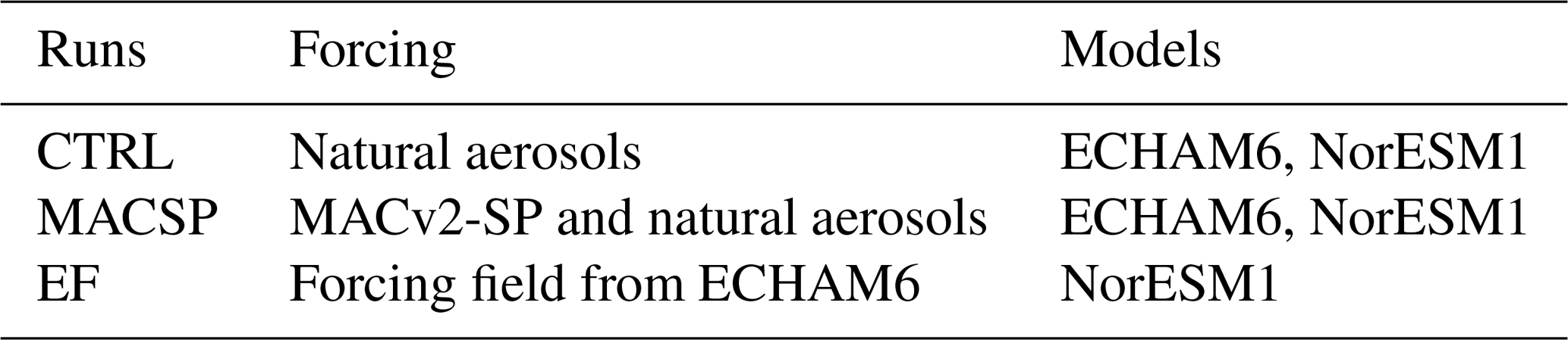
Sets of 100-year equilibrium climate runs for the year 2005 were conducted with both models, with the last 60 years used for the analysis. (1) The control run (CTRL) included only natural aerosols and was constructed from two runs for each model with small initial condition perturbations. (2) The MACSP run included both natural and anthropogenic aerosols for the year 2005. In addition, for NorESM1, a third run (EF) was carried out. This run employed the time-varying 3-D aerosol radiative forcing field computed from the ECHAM6's MACSP run. A more detailed description of the implementation is given in the Appendix A. A summary of the runs is given in Table 1.
Based on these runs, the following three experiments were defined to estimate the effect of anthropogenic aerosols: ECHAM6-MACSP (the difference between the MACSP and CTRL runs for ECHAM6), NorESM1-MACSP (MACSP minus CTRL for NorESM1) and NorESM1-EF (EF minus CTRL for NorESM1). The analysis of the results was based on monthly-mean values of data and focused on the effects of MACv2-SP aerosols on near-surface temperature, precipitation, surface albedo and total cloud cover. The statistical significance of the responses was evaluated using a Student's t test with an auto-correlation correction according to Zwiers and von Storch (1995). The response uncertainties in global-mean values were estimated by the standard error of means taking into account lag-1 auto-correlation according to Zwiers and von Storch (1995). The instantaneous radiative forcing was calculated using double radiation calls with and without MACv2-SP aerosols during the slab ocean runs.
3.1 Aerosol radiative forcing
The total radiative forcing from the MACv2-SP anthropogenic aerosol description was found to be very similar for the two models (see Fig. 1). For ECHAM6, the MACv2-SP aerosol scheme produces a global average total shortwave radiative forcing at the top of the atmosphere (TOA) for the year 2005, with arising from direct and from indirect radiative forcing. For NorESM1, the same aerosol scheme produces a slightly higher global radiative forcing of at TOA, with direct and indirect radiative forcing. Figure C1 shows the maps of aerosol direct and indirect radiative forcing in the two models as calculated here. The largest difference in the total forcing was found over southeast Asia (up to 3.20 Wm−2), where also the largest absolute forcing was found in both models. Fiedler et al. (2019) have calculated both the MACv2-SP effective radiative forcing and the instantaneous radiative forcing using double radiation calls with fixed sea surface temperature for the two climate models used here. They showed that with fixed sea surface temperature the MACv2-SP aerosols produce an instantaneous radiative forcing of −0.60 and in ECHAM6 and NorESM1, respectively. The correlation coefficient for the regional total forcing in the two models due to MACv2-SP is 0.97, and 0.90 for direct and 0.89 indirect forcing only. Thus, the regional differences in direct and indirect forcing somewhat compensate for each other.
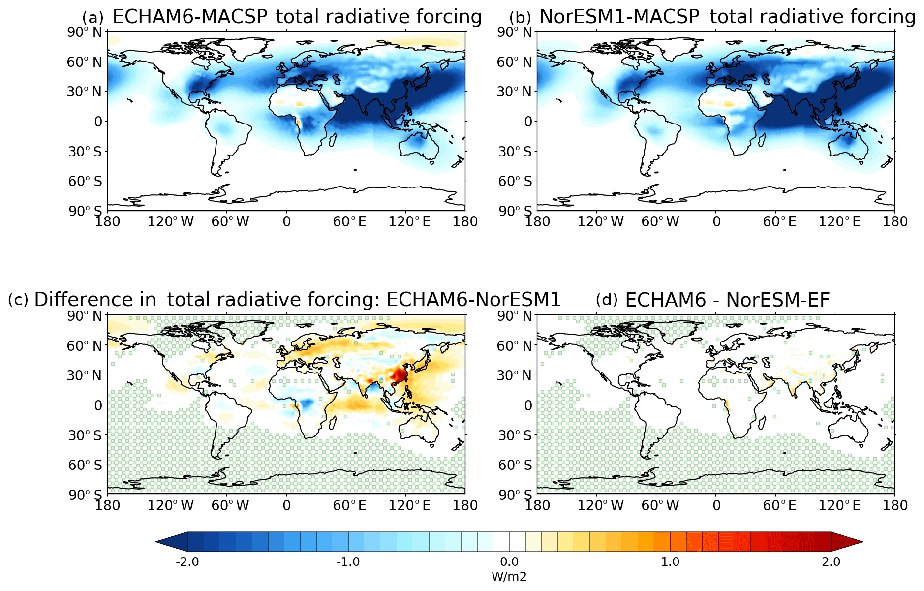
Figure 1The total radiative forcing at top of the atmosphere produced by MACv2-SP aerosols. Panel (a) shows the forcing in ECHAM6-MACSP experiment and (b) in NorESM1-MACSP experiment. Panels (c) and (d) show the difference in forcing between the two models and difference between ECHAM-MACSP and NorESM1-EF runs. Small green circles mask the areas where results are not statistically significant at the p<0.05 level.
We used a Gaussian process emulation technique (O'Hagan, 2006) to assess the causes for the regional differences in aerosol radiative forcing (see Appendix B for details). Our analysis showed that differences in cloud cover and surface albedo can explain nearly all of the variance in the difference in total instantaneous shortwave radiative forcing between ECHAM6 and NorESM1. Our sensitivity analysis reveals that in the regions with the largest radiative forcing (close to the center of the MACv2-SP plumes) the difference in model cloud cover dominates the difference in model shortwave forcing. In contrast, in regions with low aerosol radiative forcing, the differences in surface albedo dominate the differences in forcing. We note that these results apply only to fixed aerosol fields produced by the MACv2-SP representation. Previous research shows that the aerosol radiative forcing can also depend on the meteorology (surface winds and precipitation) produced by the models, partly driven by the natural variability of the climate system (Fiedler et al., 2019).
3.2 Climate response to the addition of anthropogenic aerosols
3.2.1 Temperature
We obtain a robust global temperature response of −0.5 K due to the inclusion of MACv2-SP anthropogenic aerosols in both models. For the ECHAM6-MACSP experiment, the global-mean near-surface temperature response is −0.50 (±0.03) K, with regional values ranging from +0.30 to −2.10 K. For the NorESM1-MACSP experiment, the global-mean value is −0.48 (±0.02) K and the regional values range between +0.39 and −2.28 K.

Figure 2Near-surface temperature response to the addition of anthropogenic (MACv2-SP) aerosols. Panel (a) shows the response for ECHAM6-MACSP experiment and (b) for NorESM1-MACSP experiment. Panels (c) and (d) show the difference in the responses between the two models and difference between NorESM1-MACSP and NorESM1-EF. Small green circles mask the areas where results are not statistically significant at the p<0.05 level.
Figure 2 shows the regional temperature response to the inclusion of anthropogenic MACv2-SP aerosols. The spatial correlation between ECHAM6-MACSP and NorESM1-MACSP experiments is 0.81 for full experiments with 60+120 years of MACSP and CTRL runs in both models. The largest cooling in ECHAM6 is located in southeast Asia, whereas in NorESM1 the largest cooling is found near the Russian Far East and north of Japan, with a second minimum over the Greenland Sea. Small positive temperature responses are found close to the Antarctic coast in both models, but these temperature responses are not statistically significant and are related to natural variations in sea ice. We found some significant correlation between the regional aerosol forcing and regional temperature response in both models: 0.39 in ECHAM6 and 0.29 in NorESM1, respectively. Among the CMIP5 model considered in Shindell et al. (2015), the multi-model mean regional correlation between the combined effective aerosol and ozone forcing and temperature response was slightly negative (−0.1), varying between negative values in some models and positive values among others.
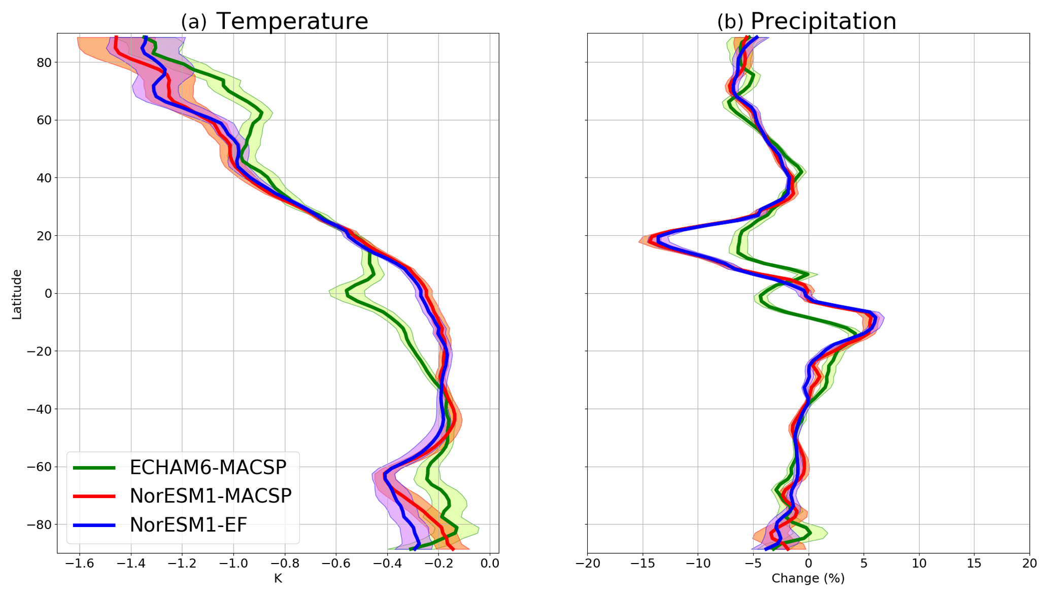
Figure 3Impact of MACSP anthropogenic aerosols on zonal-mean temperature (K) and precipitation (%) in ECHAM6-MACSP, NorESM1-MACSP and NorESM1-EF experiments. The shaded area shows the standard error of the mean as a function of latitude.
Figure 3a shows the zonal-mean temperature responses obtained from ECHAM6-MACSP and NorESM1-MACSP experiments. These experiments show a moderate cooling due to anthropogenic aerosols across the Southern Hemisphere latitudes, whereas in the Northern Hemisphere the cooling response clearly strengthens towards the high latitudes. The modeled regional temperature responses between ECHAM6 and NorESM1 simulations disagree the most in mid- and high-latitude regions, as seen in Fig. 2c. In high-latitude regions, temperature differences are associated with surface albedo responses (snow/sea ice) between the models (see Fig. C2). Changes in surface albedo are known to amplify changes in Arctic temperatures (albedo feedback). Hence, differences in snow and sea ice responses may partly explain the difference in temperature responses in the high latitudes. This feedback, together with ocean circulation feedback, also dominates at high latitudes the regional differences in temperature responses to homogeneous greenhouse gas forcing among different climate models (Shindell et al., 2015).
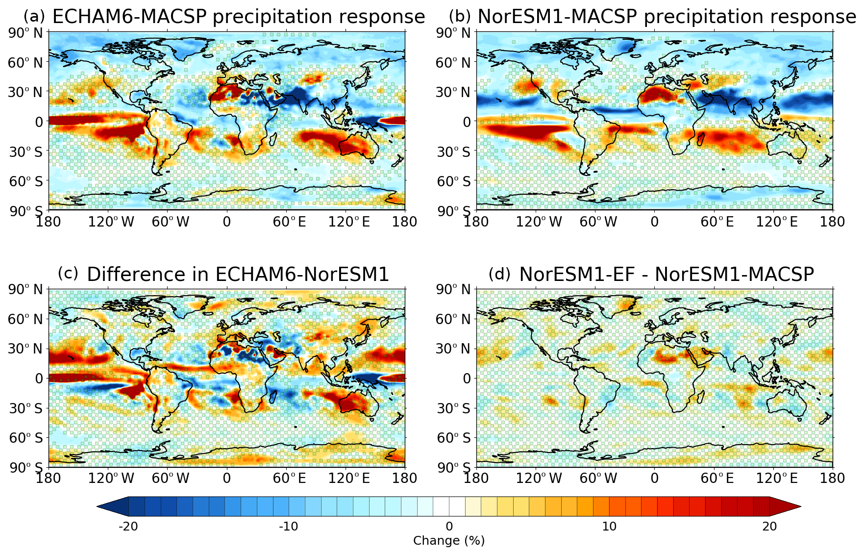
Figure 4Panel (a) shows the ECHAM6-MACSP experiment precipitation response to adding MACv2-SP aerosols and (b) shows the same for the NorESM1-MACSP experiment. Panels (c) and (d) show the intermodel difference in precipitation response and difference between NorESM1-MACSP and NorESM1-EF. The green dots mark the regions where the MACv2-SP aerosols do not have a statistically significant impact at the p<0.05 level.
3.2.2 Precipitation
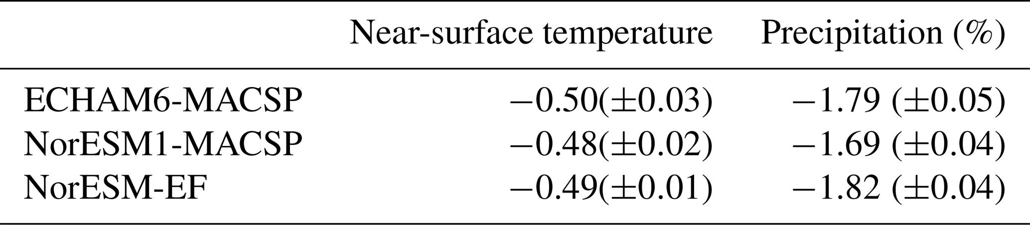
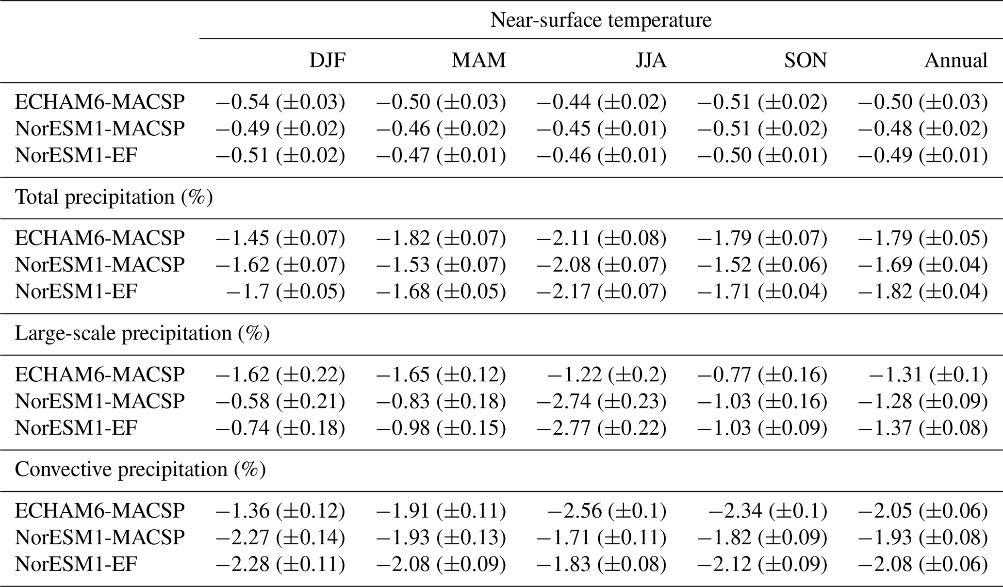
The inclusion of anthropogenic aerosols results in a similar global reduction of precipitation in all experiments, with ECHAM6-MACSP showing a change of % and NorESM1-MACSP showing a change of % in annual precipitation (Table 2). The regional changes of the precipitation patterns are shown in Fig. 4. The spatial correlation between the precipitation responses in the full ECHAM6-MACSP and NorESM1-MACSP experiments is 0.47, which is much lower than the corresponding correlation for temperature. In addition, while the temperature responses are negative almost globally, both positive and negative responses occur for precipitation, with relatively sharp edges between regions with different signs of changes. While similar large-scale features of precipitation changes can be seen in both models, their dislocation leads to a weaker regional correlation than for the temperature response. In both models, the relative changes in the convective precipitation are larger than the relative changes in large-scale precipitation. Also consistently across the two models, the seasonal response in the total precipitation is similar, with the largest changes in June–July–August (see Table C1). Both models consistently show an overall drying of the Northern Hemisphere, with some statistically significant regional increases in precipitation over northwest Africa.
Table 2Summary of modern-day global-mean change of temperature and precipitation. Standard errors of means are shown in brackets.
Both models show a maximum reduction in total precipitation around 15–20∘ N and a maximum increase around 10–15∘ S, associated with an asymmetric response in Hadley circulation across the Equator (see Figs. 3b and 4). Changes in precipitation in the tropics are also related to changes in vertical motion in the same region (see Fig. C4). This is suggestive of a southward shift of the Intertropical Convergence Zone (ITCZ) associated with a change in hemispheric temperature gradient (Broccoli et al., 2006). The inclusion of anthropogenic aerosols results in decreased precipitation in the South Asian monsoon region (defined here as the land region over 5–25∘ N, 65–110∘ E) (Fig. 3). In June–August, the monsoon precipitation decreased by 12.8 % in the ECHAM6-MACSP and 15.3 % in the NorESM1-MACSP experiments. Reduction of monsoon precipitation due to the anthropogenic aerosols has also been reported in several previous studies (Ganguly et al., 2012; Li et al., 2018b; Polson et al., 2014; Bollasina et al., 2011). In contrast with the seasonal cycle in temperature response, the largest precipitation response occurs in Northern Hemisphere summer during the Asian monsoon season. The two models show a different response over the West African monsoon region (5∘ S–25∘ N, 20∘ W–20∘ E), with the NorESM1-MACSP experiment showing a statistically significant reduction in precipitation of −5.3 %, while the ECHAM6-MACSP experiment does not show a significant change (−1.8 %). In the vicinity of the Australian continent, the ECHAM6-MACSP experiment shows an area of increased precipitation extending from the Indian Ocean to western Australia, while in the NorESM1-MACSP experiment, the increase is located entirely over the Indian Ocean.
There appear to be several causes for the differences in the precipitation response between the two models. For instance, there is a relationship between the difference of the regional precipitation response and the difference in vertical velocity response (correlation coefficient 0.44 between Figs. 4c and C4c). However, it cannot be concluded that change in precipitation is caused by the change in vertical velocity. Probably, both the changes in vertical velocity and precipitation are related to changes in circulation. Also the difference in the initial equilibrium state of precipitation patterns correlates weakly with the difference in the precipitation response (correlation coefficient 0.23). Furthermore, differences in the cloud cover responses (see Fig. C3) are also related to differences in precipitation responses (correlation coefficient 0.32). The vertical velocity correlates also with the total cloud cover response (correlation coefficient 0.41).
3.2.3 Comparison between the NorESM1-MACSP and NorESM1-EF experiments
We now briefly discuss the differences between the NorESM1-MACSP and NorESM1-EF experiments. As noted in Sect. 2.3, the difference between these experiments is that in NorESM1-MACSP, the radiative forcing due to the MACv2-SP aerosols is computed using NorESM1's own meteorology and own radiation scheme, while in NorESM1-EF, forcing from ECHAM6's MACSP run is applied. The forcing results are shown in Fig. 1d. The minor differences seen in Fig. 1d are related to interpolating the radiative forcing between ECHAM6 and NorESM1 horizontal grids. The general finding here is that the results for these two experiments are very similar. The global-mean temperature response is −0.48 (±0.02) K for NorESM1-MACSP and −0.49 (±0.01) K for NorESM1-EF, while the global-mean precipitation responses are −1.69 (±0.04) % and −1.82 (±0.04) %. Also, the zonal-mean and regional temperature and precipitation responses in NorESM1-MACSP and NorESM1-EF are very similar (Figs. 2d, 3 and 4d). The spatial correlation in response between the full NorESM1-MACSP and NorESM1-EF experiments is as high as 0.97 for temperature and 0.95 for precipitation, which are much higher than the correlations between NorESM1-MACSP and ECHAM6-MACSP responses (0.81 and 0.47). Indeed, with the exception of the global-mean precipitation response, for which the ECHAM6-MACSP value (−1.79 ±0.05 %) falls between NorESM1-MACSP and NorESM1-EF, the responses in the two NorESM1 experiments are closer to each other than the ECHAM6-MACSP response. Therefore, it can be concluded that the differences in the effects of MACv2-SP aerosols between ECHAM6 and NorESM1 are mainly related to differences in the model circulation responses, not to the differences in the aerosol forcing fields.
3.3 Comparison to models with interactive aerosols
Finally, we compare the obtained equilibrium temperature and precipitation responses with prescribed MACv2-SP aerosols in ECHAM6 and NorESM1 against those equilibrium climate responses from four fully coupled climate models (CESM1, GISS, HadGEMS2 and NorESM1) with intrinsic aerosol schemes but the same aerosol emissions, reported by Samset et al. (2018). In the four models considered by Samset et al. (2018), the global average temperature responses were −(0.5, 0.5, 1.1 and 0.6) K, and precipitation responses were −(1.5 %, 1.8 %, 2.6 % and 3.1 %), respectively. We obtain similar temperature responses of −(0.48–0.50) K and precipitation responses of −(1.69–1.82) % using the prescribed MACv2-SP aerosol description.
Table 3Intermodel correlations of regional temperature response for the Samset et al. (2018) models and our models. The average correlation coefficient between the Samset et al. (2018) models is 0.79 with a standard deviation of 0.05; the average correlation coefficient between the models used in this study and the Samset et al. (2018) models is 0.76. The correlations are calculated for 50 years with and 50 years without anthropogenic aerosols. Correlation for our whole dataset (60+120 years) is shown in brackets. The range is the standard deviation between results obtained for two different CTRL runs.
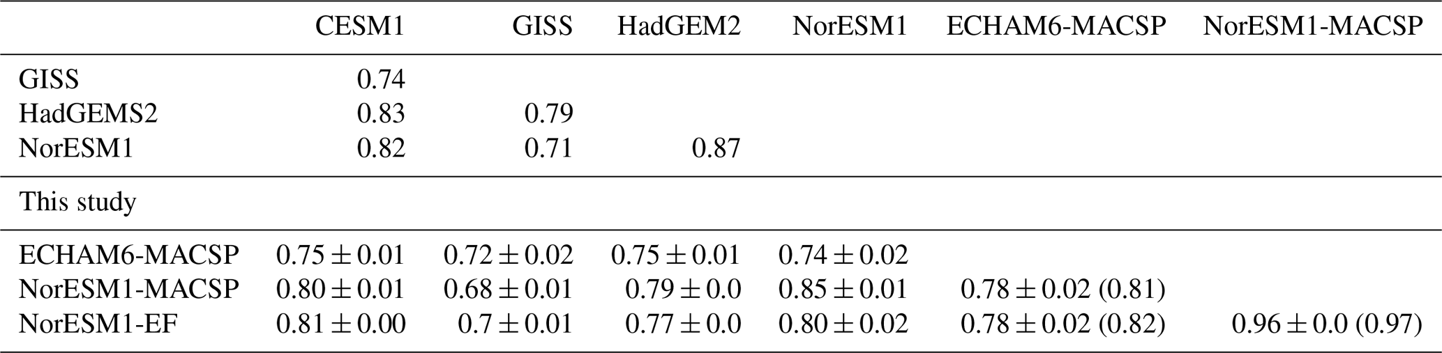
Table 4Intermodel correlations of regional precipitation response for the Samset et al. (2018) models and our models. The average correlation coefficient between the models is 0.34 with a standard deviation of 0.10; the average correlation coefficient between the models used in this study and the Samset et al. (2018) models is 0.38. The correlations are calculated for 50 years with and 50 years without anthropogenic aerosols. The range of the correlation coefficient shows the standard deviations between results obtained for two different CTRL runs. The correlation for our whole dataset (60+120 years) is shown in brackets.

Tables 3 and 4 show the correlation coefficients for regional climate responses between all experiments in our datasets and the Samset et al. (2018) datasets. The correlations are calculated for equilibrium climate runs with equal time averaging over 50 years with and without anthropogenic aerosols both for our datasets and the Samset et al. (2018) datasets. Note that these coefficients do not depend on the magnitude of the average responses in the models but only on the relative regional distributions of the responses. Perhaps surprisingly, the average correlation coefficient for regional temperature response between interactive aerosol models (i.e., the Samset et al., 2018 models), 0.79, is almost identical to the correlation between our prescribed aerosol models (0.78). Also, the average correlation coefficient between experiments using interactive aerosols and a fully coupled ocean model (Samset et al., 2018) and experiments using prescribed aerosols and a slab ocean model (our models) is 0.76, nearly the same as for the fully coupled interactive aerosol models only. The similar regional correlation between different experiments is remarkable considering large differences in the aerosol descriptions between the different models. It appears that the differences in aerosol descriptions do not dominate the differences in regional temperature response. The average correlation coefficient for regional precipitation changes within Samset et al. (2018) models with intrinsic aerosol descriptions is 0.34, while it is 0.41 within our models with prescribed aerosols. The average correlation coefficient for regional precipitation changes between the Samset et al. (2018) models with fully coupled ocean and our models with a slab ocean is 0.39, which is similar to the mean correlation within the Samset et al. (2018) models.
The correlation coefficient between NorESM1 experiments using different aerosol descriptions and ocean models is now only 0.33∕0.38. Thus, differences in aerosol descriptions, ocean models and atmospheric responses all contribute to differences in regional precipitation responses. The correlation coefficients for precipitation responses are, however, more uncertain than those for temperature responses, due to a stronger impact of natural variability.
Even long equilibrium climate runs cannot fully eliminate the natural climate variability on a regional level. With our full dataset (60 years of MACSP runs +120 years of the CTRL run), we obtain a spatial correlation of 0.47 between NorESM1-MACSP and ECHAM6-MACSP precipitation responses, a slight improvement over the correlation coefficient of 0.41 (±0.02) for 50+50-year datasets. The spatial correlation for temperature improves from 0.78 (±0.02) to 0.81. The fully coupled ocean models in the Samset et al. (2018) dataset also feature long-term internal variability in the ocean states that adds to the level of natural variation with respect to our models with simpler slab ocean representations used in this paper. Therefore, we would expect the Samset et al. (2018) data to include more noise than our results with slab ocean configurations. Furthermore, it is important to note that differences in the ocean descriptions are known to have a large impact in the regional climate responses between different models (Deser et al., 2016; Kay et al., 2016). Overall, we would expect that due to these differences the climate signals obtained from fully coupled models would intrinsically correlate less well with each other than those from models with slab ocean configurations. Somewhat surprisingly, this turns out not to be the case.
The dependence of the calculation of time-averaged correlation coefficients on the simulation length for our data is shown in Fig. 5. There, the blue and red shaded regions represent the level of expected variation in the regional correlation coefficients between two climate models obtained from equilibrium model experiments with and without anthropogenic aerosols. We obtained a correlation coefficient of 0.78 with a standard deviation of ±0.02 for temperature response and 0.41 (±0.02) for precipitation after 50 years of simulation, these periods being representative for the Samset experiments but neglecting the impact of long-term ocean variations. The corresponding correlation coefficients for full model runs (60+120 years of simulation) are 0.47 for precipitation and 0.81 for temperature.

Figure 5Correlation coefficient of temperature (precipitation) response as a function of the number of averaged years. Blue (red) is the correlation between the temperature responses to MACv2-SP aerosols in the two models. The shaded area shows the variation between different control runs. The same number of years is used for the CTRL run and MACSP run.
We have provided results here on the equilibrium climate response of modern-day anthropogenic aerosols using two different climate models, ECHAM6 and NorESM1, with the MACv2-SP (Stevens et al., 2017) anthropogenic aerosol representations. The results were obtained both using the same representations of aerosol optical properties and cloud–albedo effect and for identical instantaneous aerosol radiative forcing fields in the models.
The MACv2-SP aerosols produced a very similar total instantaneous anthropogenic aerosol radiative forcing in the two models ( in the ECHAM6-MACSP and in the NorESM1-MACSP experiments). We found that there are differences up to 3.2 Wm−2 in the instantaneous regional aerosol forcing between the models when using the same aerosol representation. These differences can mostly be explained via differences in cloud fields and surface albedo in the models.
The addition of MACv2-SP anthropogenic aerosols produced very similar global average responses on temperature, −0.48 (±0.02) and −0.50 (±0.03) K, and precipitation, −1.69 (±0.04) % and −1.79 (±0.05) % in the NorESM1-MACSP and ECHAM6-MACSP experiments, respectively. The largest disagreement in regional temperature response was found at high-latitude regions associated with largest differences in surface albedo feedback (snow/sea ice), while the largest differences in regional precipitation response were located mainly in the tropics. These key regional differences remained even when using exactly the same aerosol radiative forcing fields in both models. Several previous studies have discussed that the main driver for ITCZ shift is the Northern Hemisphere cooling due to anthropogenic aerosols (Broccoli et al., 2006; Hwang et al., 2013; Wang, 2015). Chiang and Bitz (2005) showed with the Community Climate Model version 3 a connection between ITCZ shift and added Arctic ice cover. Based on these previous studies, it seems plausible that different responses in Arctic sea ice and snow cover in ECHAM6-MACSP and in the two NorESM1 experiments result in different high-latitude temperature responses, which in turn are reflected as differences in the ITCZ shift that drives the precipitation change at low latitudes. However, it should be noted that the ITCZ shift is also sensitive to the type of ocean model used, and slab ocean models tend to exaggerate the change in ITCZ (Kay et al., 2016).
We compared our results using uniform aerosol representations to a set of four current climate models using their intrinsic aerosol representations but the same aerosol emissions, reported by Samset et al. (2018). Among the Samset et al. (2018) models, the global responses to additions of anthropogenic aerosol varied between −0.5 and −1.1 K for temperature and between −1.5 % and −3.1 % for precipitation. However, the correlation coefficients for regional distributions of climate responses, averaged over equal run length, were nearly as good among our experiments with prescribed aerosols and slab ocean representation (0.78 for temperature and 0.41 for precipitation) and among the Samset et al. experiments with model-intrinsic aerosols and the fully coupled ocean representation (0.79 for temperature and 0.34 for precipitation).
The lack of improvement in the correlation coefficients suggests that differences in aerosol descriptions are not the only cause of regional differences in climate signals between the models. Rather, the differences in model circulation responses appear to dominate the differences in regional climate responses. Figure C5 shows the average 850 hPa wind responses for the ECHAM6-MACSP and NorESM1-MACSP experiments for Northern Hemisphere winter. The responses in the circulation fields vary significantly between the two models, with an annual average correlation coefficient of only 0.18 (DJF: −0.03; MAM: 0.07; JJA: 0.15; SON: 0.19). The lack of robustness in atmospheric circulation responses between different climate models has been previously discussed by Shepherd (2014) for CMIP5 Representative Concentration Pathway (RCP) 8.5 scenarios and by Li et al. (2018a) for HAPPI (Half a degree Additional warming, Prognosis and Projected Impact) 1.5 and 2.0 K warming scenarios. Shepherd (2014) argued that the differences in circulation responses cause variation in the regional temperature and precipitation responses in future climate scenarios. Li et al. (2018a) showed that model consensus for circulation response is low even for atmosphere-only models forced with same time-varying sea surface temperature (SST) and sea ice, anthropogenic greenhouse gases, ozone, land use, land cover and aerosols. Both in Shepherd (2014) and Li et al. (2018a) data, the NH wintertime circulation response over the North Atlantic disagrees significantly between models. Also for ECHAM6-MACSP and NorESM1-MACSP, the circulation response over the North Atlantic shows differences in magnitude and pattern. Differences are also seen over the North Pacific region. Combined with the difference in the sea ice and surface albedo change in the North Pacific, these circulation changes can drive the temperature response differences in the region.
Our results imply that in current global climate models the regional aerosol climate impacts cannot be better constrained by further improving aerosol descriptions alone. More extensive model comparisons are needed to explain the model discrepancies in response to aerosol forcing. Improvements on the dynamical cores, physical parameterizations and ocean models are needed to narrow down model uncertainties in the regional aerosol climate responses.
Data and scripts are available at https://etsin.fairdata.fi/dataset/7cf4b0d1-7789-4756-b7bc-3964d0646a4c (Nordling et al., 2019).
The NorESM1-EF run employed radiative forcing extracted from the ECHAM6-MACSP run. First, multi-year monthly means of MACv2-SP aerosol radiative forcing (for TOA and surface radiative fluxes and atmospheric heating rates) were computed for ECHAM6-MACSP. Second, these values were interpolated to the NorESM1 horizontal and vertical grid and normalized by the monthly-mean incoming solar radiation at model top. Third, during the NorESM1-EF run, the normalized forcing was multiplied by the TOA incoming solar radiation at each radiation time step, and it was added to the radiative fluxes and heating rates computed without MACv2-SP aerosols.
This treatment ensures that the diurnal cycle of the aerosol forcing is approximately correct; in particular, there is no aerosol forcing during the night. However, the computed forcing is independent of the clouds simulated by NorESM1. Thus, while the aerosol radiative forcing is computed correctly in a monthly-mean sense, its sub-monthly correlation with clouds is ignored. In principle, this could impact the differences between NorESM1-EF and ECHAM6-MACSP. The impact is, however, most likely small. If neglecting the sub-monthly correlation between clouds and aerosol forcing were to have a substantial impact on the climate response to MACv2-SP aerosols, this should also show up in the differences between NorESM1-EF and NorESM1-MACSP. Yet, the differences between NorESM1-EF and NorESM1-MACSP are very small (Tables 2 and C1), in fact much smaller than the corresponding differences between ECHAM6-MACSP and either NorESM1-EF or NorESM1-MACSP. This strongly suggests that the differences between NorESM1-EF and ECHAM6-MACSP are primarily caused by the use of a different climate model rather than by the subtle differences in radiative forcing.
We used a Gaussian process emulation technique (O'Hagan, 2006) to evaluate the regional differences in aerosol radiative forcing. First, we simply assume that the forcing difference depends only on the differences in model output values and not on the actual values themselves. Second, we selected the differences in modeled output (total cloud cover, surface albedo, precipitation, surface temperature, surface wind u component) as trial sets for these values. These can be described via a relation Y=η(X), where , where α and β are total cloud cover and surface albedo, and ξ is a pure noise (Gaussian) variable. Next, the function Y=η(X) is inferred using a Gaussian process prior emulator for a part of the yearly averaged radiative forcing data (in our case, 40 years). Each variable is assigned a sensitivity index which describes the relative sensitivity of Y to that variable. The sensitivity analysis of the estimated Y function was done by using the extended Fourier amplitude sensitivity test (FAST) (Saltelli et al., 1999). As an end result, FAST assesses the contributions of each emulator input variable (components of X=(Xi)) to the variance in emulator output variable (Y), where it is assumed the input variables Xi have an independent and identical distribution uniform prior. The inferred function Y is finally validated by comparing the emulated forcing field against validation data separate from the training data (here, 20 years long, constructed from 20-year monthly values).
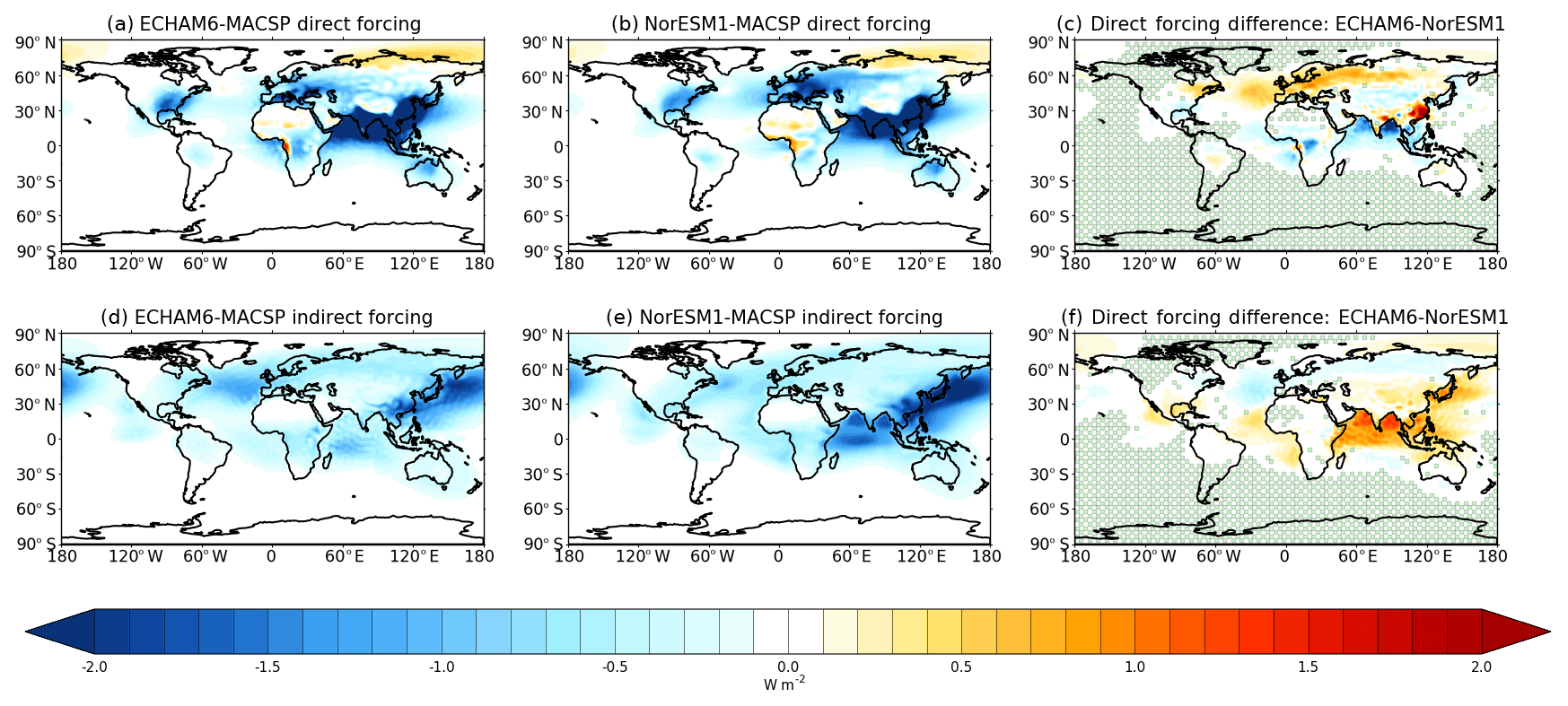
Figure C1Instantaneous radiative forcing by anthropogenic (MACv2-SP) aerosols. Panels (a), (b), (c) show the direct radiative forcing, and (d), (e), (f) show the indirect radiative forcing produced by MACv2-SP. Green masking in panels (c) and (f) indicates areas where the difference between the models in the instantaneous radiative forcing is not statistically significant (p>0.05).

Figure C2Surface albedo response to the addition of anthropogenic aerosols. (a) Response in the ECHAM6-MACSP experiment; (b) response in the NorESM1-MACSP experiment; (c) the difference in surface albedo response: ECHAM6-MACSP experiment minus NorESM1-MACSP experiment. The green dots represent the area where anthropogenic aerosols do not have a statistically significant impact at the p<0.05 level (in panel c) or where the difference between the models is not statistically significant (in panels a and b).

Figure C3Total cloud cover response to the addition of anthropogenic aerosols. (a) Response in the ECHAM6-MACSP experiment; (b) response in the NorESM1-MACSP experiment; (c) the difference in responses between the experiments. The green dots represent the area where anthropogenic aerosols do not have a statistically significant impact at the p<0.05 level (in panel c) or where the difference between the models is not statistically significant (in panels a and b).
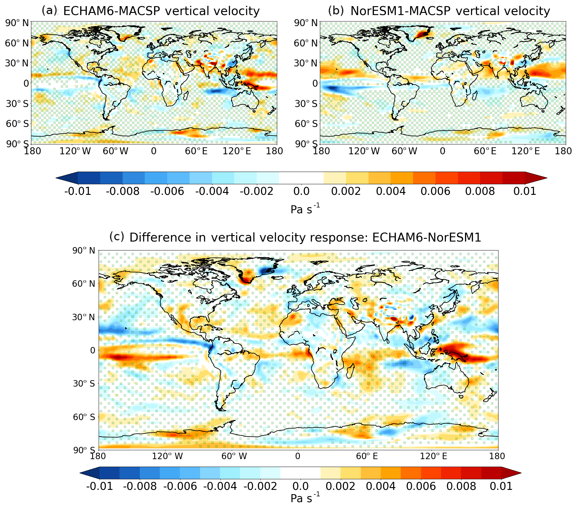
Figure C4Vertical motion response at the 600 hPa level to the addition of anthropogenic aerosols. (a) Response in the ECHAM6-MACSP experiment; (b) response in the NorESM1-MACSP experiment; (c) the difference in responses between the experiments. The green dots represent the area where anthropogenic aerosols do not have a statistically significant impact at the p<0.05 level (in panel c) or where the difference between the models is not statistically significant (in panels a and b).

Figure C5Lower tropospheric (850 hPa) zonal wind response to adding MACv2-SP anthropogenic aerosols for Northern Hemisphere winter. The green dots represent the area where anthropogenic aerosols do not have a statistically significant impact at the p<0.05 level (in panel c) or where the difference between the models is not statistically significant (in panels a and b). The units are in m s−1.
Table C1Summary of global-mean change of temperature and precipitation due to modern-day anthropogenic aerosols. Error bars are the standard error of means.
KN performed ECHAM6 simulations with help from JM, PR and DO'D. PR performed all NorESM1 simulations. MEA advised on the sensitivity analysis. PU advised on the data analysis. The manuscript was written by KN and JM, with contributions from all authors. HK came up with the initial research idea and JM coordinated the project.
The authors declare that they have no conflict of interest.
This project has been funded by the European Research Council (ERC) under the European Union's Horizon 2020 research and innovation program under grant agreement no. 646857, and by the Academy of Finland (project 287440). Petteri Uotila was supported by the EC Marie Curie Support Action LAWINE (grant 707262). The authors would also like to thank Bjørn Hallvard Samset for providing data of fully coupled model runs, Stephanie Fiedler for providing MACv2-SP code for ECHAM6.1 and two reviewers for reviewing this paper.
This research has been supported by the Academy of Finland (grant no. 287440), the EC Marie Curie Support Action LAWINE (grant no. 707262) and the European Research Council (grant no. 646857).
This paper was edited by Peter Haynes and reviewed by Peter Haynes and one anonymous referee.
Bentsen, M., Bethke, I., Debernard, J. B., Iversen, T., Kirkevåg, A., Seland, ø., Drange, H., Roelandt, C., Seierstad, I. A., Hoose, C., and Kristjánsson, J. E.: The Norwegian Earth System Model, NorESM1-M – Part 1: Description and basic evaluation of the physical climate, Geosci. Model Dev., 6, 687–720, https://doi.org/10.5194/gmd-6-687-2013, 2013. a
Bollasina, M. A., Ming, Y., and Ramaswamy, V.: Anthropogenic Aerosols and the Weakening of the South Asian Summer Monsoon, Science, 334, 502–505, 2011. a, b
Boucher, O., Randall, D., Artaxo, P., Bretherton, C., Feingold, G., Forster, P., Kerminen, V.-M., Kondo, Y., Liao, H., Lohmann, U., Rasch, P., K. Satheesh, S., Sherwood, S., Stevens, B., and Zhang, X.: Clouds and Aerosols, in: Climate Change 2013: The Physical Science Basis, Contribution of Working Group I to the Fifth Assessment Report of the Intergovernmental Panel on Climate Change, edited by: Stocker, T. F., Qin, D., Plattner, G.-K., Tignor, M., Allen, S. K., Boschung, J., Nauels, A., Xia, Y., Bex, V., and Midgley, P. M., Cambridge University Press, Cambridge, United Kingdom and New York, NY, USA a
Broccoli, A. J., Dahl, K. A., and Stouffer, R. J.: Response of the ITCZ to Northern Hemisphere cooling, Geophys. Res. Lett., 33, L01702, https://doi.org/10.1029/2005GL024546, 2006. a, b
Carslaw, K. S., Lee, L. A., Reddington, C. L., Pringle, K. J., Rap, A., Forster, P. M., Mann, G. W., Spracklen, D. V., Woodhouse, M. T., Regayre, L. A., and Pierce, J. R.: Large contribution of natural aerosols to uncertainty in indirect forcing, Nature, 503, 67–71, https://doi.org/10.1038/nature12674, 2013. a
Chiang, J. C. H. and Bitz, C. M.: Influence of high latitude ice cover on the marine Intertropical Convergence Zone, Clim. Dynam., 25, 477–496, https://doi.org/10.1007/s00382-005-0040-5, 2005. a
Deser, C., Sun, L., Tomas, R. A., and Screen, J.: Does ocean coupling matter for the northern extratropical response to projected Arctic sea ice loss?, Geophys. Res. Lett., 43, 2149–2157, https://doi.org/10.1002/2016GL067792, 2016. a
Ekman, A. M. L.: Do sophisticated parameterizations of aerosol-cloud interactions in CMIP5 models improve the representation of recent observed temperature trends?, J. Geophys. Res.-Atmos., 119, 817–832, https://doi.org/10.1002/2013JD020511, 2014. a
Feser, F., Rockel, B., von Storch, H., Winterfeldt, J., Zahn, M., Feser, F., Rockel, B., Storch, H. v., Winterfeldt, J., and Zahn, M.: Regional Climate Models Add Value to Global Model Data: A Review and Selected Examples, B. Am. Meteorol. Soc., 92, 1181–1192, https://doi.org/10.1175/2011BAMS3061.1, 2011. a
Fiedler, S., Kinne, S., Huang, W. T. K., Räisänen, P., O'Donnell, D., Bellouin, N., Stier, P., Merikanto, J., van Noije, T., Makkonen, R., and Lohmann, U.: Anthropogenic aerosol forcing – insights from multiple estimates from aerosol-climate models with reduced complexity, Atmos. Chem. Phys., 19, 6821–6841, https://doi.org/10.5194/acp-19-6821-2019, 2019. a, b
Ganguly, D., Rasch, P. J., Wang, H., and Yoon, J.-H.: Climate response of the South Asian monsoon system to anthropogenic aerosols, J. Geophys. Res.-Atmos., 117, https://doi.org/10.1029/2012JD017508, 2012. a
Giorgi, F. and Francisco, R.: Uncertainties in regional climate change prediction: a regional analysis of ensemble simulations with the HADCM2 coupled AOGCM, Clim. Dynam., 16, 169–182, https://doi.org/10.1007/PL00013733, 2000. a
Hawkins, E., Smith, R. S., Gregory, J. M., and Stainforth, D. A.: Irreducible uncertainty in near-term climate projections, Clim. Dynam., 46, 3807–3819, https://doi.org/10.1007/s00382-015-2806-8, 2016. a
Hwang, Y.-T., Frierson, D. M. W., and Kang, S. M.: Anthropogenic sulfate aerosol and the southward shift of tropical precipitation in the late 20th century, Geophys. Res. Lett., 40, 2845–2850, https://doi.org/10.1002/grl.50502, 2013. a
Iversen, T., Bentsen, M., Bethke, I., Debernard, J. B., Kirkevåg, A., Seland, Ø., Drange, H., Kristjansson, J. E., Medhaug, I., Sand, M., and Seierstad, I. A.: The Norwegian Earth System Model, NorESM1-M – Part 2: Climate response and scenario projections, Geosci. Model Dev., 6, 389–415, https://doi.org/10.5194/gmd-6-389-2013, 2013. a
Kasoar, M., Voulgarakis, A., Lamarque, J.-F., Shindell, D. T., Bellouin, N., Collins, W. J., Faluvegi, G., and Tsigaridis, K.: Regional and global temperature response to anthropogenic SO2 emissions from China in three climate models, Atmos. Chem. Phys., 16, 9785–9804, https://doi.org/10.5194/acp-16-9785-2016, 2016. a
Kay, J. E., Wall, C., Yettella, V., Medeiros, B., Hannay, C., Caldwell, P., Bitz, C., Kay, J. E., Wall, C., Yettella, V., Medeiros, B., Hannay, C., Caldwell, P., and Bitz, C.: Global Climate Impacts of Fixing the Southern Ocean Shortwave Radiation Bias in the Community Earth System Model (CESM), J. Clim., 29, 4617–4636, https://doi.org/10.1175/JCLI-D-15-0358.1, 2016. a, b
Kinne, S., O'Donnel, D., Stier, P., Kloster, S., Zhang, K., Schmidt, H., Rast, S., Giorgetta, M., Eck, T. F., and Stevens, B.: MAC-v1: A new global aerosol climatology for climate studies, J. Adv. Model. Earth Sy., 5, 704–740, https://doi.org/10.1002/jame.20035, 2013. a
Kirkevåg, A., Iversen, T., Seland, Ø., Hoose, C., Kristjánsson, J. E., Struthers, H., Ekman, A. M. L., Ghan, S., Griesfeller, J., Nilsson, E. D., and Schulz, M.: Aerosol-climate interactions in the Norwegian Earth System Model – NorESM1-M, Geosci. Model Dev., 6, 207–244, https://doi.org/10.5194/gmd-6-207-2013, 2013. a
Lamarque, J.-F., Bond, T. C., Eyring, V., Granier, C., Heil, A., Klimont, Z., Lee, D., Liousse, C., Mieville, A., Owen, B., Schultz, M. G., Shindell, D., Smith, S. J., Stehfest, E., Van Aardenne, J., Cooper, O. R., Kainuma, M., Mahowald, N., McConnell, J. R., Naik, V., Riahi, K., and van Vuuren, D. P.: Historical (1850–2000) gridded anthropogenic and biomass burning emissions of reactive gases and aerosols: methodology and application, Atmos. Chem. Phys., 10, 7017–7039, https://doi.org/10.5194/acp-10-7017-2010, 2010. a
Li, C., Michel, C., Seland Graff, L., Bethke, I., Zappa, G., Bracegirdle, T. J., Fischer, E., Harvey, B. J., Iversen, T., King, M. P., Krishnan, H., Lierhammer, L., Mitchell, D., Scinocca, J., Shiogama, H., Stone, D. A., and Wettstein, J. J.: Midlatitude atmospheric circulation responses under 1.5 and 2.0 ∘C warming and implications for regional impacts, Earth Syst. Dynam., 9, 359–382, https://doi.org/10.5194/esd-9-359-2018, 2018a. a, b, c
Li, X., Ting, M., and Lee, D. E.: Fast Adjustments of the Asian Summer Monsoon to Anthropogenic Aerosols, Geophys. Res. Lett., 45, 1001–1010, https://doi.org/10.1002/2017GL076667, 2018b. a
Nordling, K., Merikanto, J., Räisänen, P., Korhonen, H., Uotila, P., O'Donnell, D., and Alper, M. E.: RECIA, available at: https://etsin.fairdata.fi/dataset/7cf4b0d1-7789-4756-b7bc-3964d0646a4c last access: 12 July 2019.
O'Hagan, A.: Bayesian analysis of computer code outputs: A tutorial, Reliab. Eng. Syst. Safe., 91, 1290–1300, https://doi.org/10.1016/J.RESS.2005.11.025, 2006. a, b
Polson, D., Bollasina, M., Hegerl, G. C., and Wilcox, L. J.: Decreased monsoon precipitation in the Northern Hemisphere due to anthropogenic aerosols, Geophys. Res. Lett., 41, 6023–6029, https://doi.org/10.1002/2014GL060811, 2014. a
Ramanathan, P. J., Crutzen J. T., and Kiehl, D. R.: Aerosols, Climate, and the Hydrological Cycle, Science, 294, 2119–2124, 2005. a
Saltelli, A., Tarantola, S., and Chan, K. P.-S.: A Quantitative Model-Independent Method for Global Sensitivity Analysis of Model Output, Technometrics, 41, 39–56, https://doi.org/10.2307/1270993, 1999. a
Salzmann, M., Weser, H., and Cherian, R.: Robust response of Asian summer monsoon to anthropogenic aerosols in CMIP5 models, J. Geophys. Res.-Atmos., 119, 321–11, https://doi.org/10.1002/2014JD021783, 2014. a
Samset, B. H., Sand, M., Smith, C. J., Bauer, S. E., Forster, P. M., Fuglestvedt, J. S., Osprey, S., and Schleussner, C.-F.: Climate Impacts From a Removal of Anthropogenic Aerosol Emissions, Geophys. Res. Lett., 45, 1020–1029, https://doi.org/10.1002/2017GL076079, 2018. a, b, c, d, e, f, g, h, i
Shindell, D. T., Faluvegi, G., Rotstayn, L., and Milly, G.: Spatial patterns of radiative forcing and surface temperature response, J. Geophys. Res.-Atmos., 120, 5385–5403, https://doi.org/10.1002/2014JD022752, 2015. a, b, c
Stevens, B., Giorgetta, M., Esch, M., Mauritsen, T., Crueger, T., Rast, S., Salzmann, M., Schmidt, H., Bader, J., Block, K., Brokopf, R., Fast, I., Kinne, S., Kornblueh, L., Lohmann, U., Pincus, R., Reichler, T., and Roeckner, E.: Atmospheric component of the MPI-M Earth System Model: ECHAM6, J. Adv. Model. Earth Sy., 5, 146–172, https://doi.org/10.1002/jame.20015, 2013. a
Stevens, B., Fiedler, S., Kinne, S., Peters, K., Rast, S., Müsse, J., Smith, S. J., and Mauritsen, T.: MACv2-SP: a parameterization of anthropogenic aerosol optical properties and an associated Twomey effect for use in CMIP6, Geosci. Model Dev., 10, 433–452, https://doi.org/10.5194/gmd-10-433-2017, 2017. a, b, c, d
Stier, P., Schutgens, N. A. J., Bellouin, N., Bian, H., Boucher, O., Chin, M., Ghan, S., Huneeus, N., Kinne, S., Lin, G., Ma, X., Myhre, G., Penner, J. E., Randles, C. A., Samset, B., Schulz, M., Takemura, T., Yu, F., Yu, H., and Zhou, C.: Host model uncertainties in aerosol radiative forcing estimates: results from the AeroCom Prescribed intercomparison study, Atmos. Chem. Phys, 13, 3245–3270, https://doi.org/10.5194/acp-13-3245-2013, 2013. a
Wang, C.: Anthropogenic aerosols and the distribution of past large-scale precipitation change, Geophys. Res. Lett., 42, 10876–10884, https://doi.org/10.1002/2015GL066416, 2015. a, b
Wilcox, L. J., Highwood, E. J., Booth, B. B. B., and Carslaw, K. S.: Quantifying sources of inter-model diversity in the cloud albedo effect, Geophys. Res. Lett., 42, 1568–1575, https://doi.org/10.1002/2015GL063301, 2015. a
Zwiers and von Storch: Taking Serial Correlation into Account in Tests of the Mean, J. Clim., 8, 336–351, 1995. a, b