the Creative Commons Attribution 4.0 License.
the Creative Commons Attribution 4.0 License.
 | 24 Jan 2019
Positive matrix factorization of organic aerosol: insights from a chemical transport model
Anthoula D. Drosatou
Ksakousti Skyllakou
Georgia N. Theodoritsi
Spyros N. Pandis
Factor analysis of aerosol mass spectrometer measurements (organic aerosol mass spectra) is often used to determine the sources of organic aerosol (OA). In this study we aim to gain insights regarding the ability of positive matrix factorization (PMF) to identify and quantify the OA sources accurately. We performed PMF and multilinear engine (ME-2) analysis on the predictions of a state-of-the-art chemical transport model (PMCAMx-SR, Particulate Matter Comprehensive Air Quality Model with extensions – source resolved) during a photochemically active period for specific sites in Europe in an effort to interpret the diverse factors usually identified by PMF analysis of field measurements. Our analysis used the predicted concentrations of 27 OA components, assuming that each of them is “chemically different” from the others.
The PMF results based on the chemical transport model predictions are quite consistent (same number of factors and source types) with those of the analysis of AMS measurements. The estimated uncertainty of the contribution of fresh biomass burning is less than 30 % and of the other primary sources less than 40 %, when these sources contribute more than 20 % to the total OA. The PMF uncertainty increases for smaller source contributions, reaching a factor of 2 or even 3 for sources which contribute less than 10 % to the OA.
One of the major questions in PMF analysis of AMS measurements concerns the sources of the two or more oxygenated OA (OOA) factors often reported in field studies. Our analysis suggests that these factors include secondary OA compounds from a variety of anthropogenic and biogenic sources and do not correspond to specific sources. Their characterization in the literature as low- and high-volatility factors is probably misleading, because they have overlapping volatility distributions. However, the average volatility of the one often characterized as a low-volatility factor is indeed lower than that of the other (high-volatility factor). Based on the analysis of the PMCAMx-SR predictions, the first oxygenated OA factor includes mainly highly aged OA transported from outside Europe, but also highly aged secondary OA from precursors emitted in Europe. The second oxygenated OA factor contains fresher secondary organic aerosol from volatile, semivolatile, and intermediate volatility anthropogenic and biogenic organic compounds. The exact contribution of these OA components to each OA factor depends on the site and the prevailing meteorology during the analysis period.
- Article
(4428 KB) -
Supplement
(1692 KB) - BibTeX
- EndNote


Exposure to high levels of fine atmospheric particles results in increased mortality and morbidity (Pope et al., 2009). The same particles affect climate by scattering and absorbing solar radiation (Seinfeld and Pandis, 2006) and also influence the properties and lifetime of clouds (IPCC, 2014). Organic aerosol (OA) represents an important fraction (20 % to 90 %) of fine particulate matter (Kanakidou et al., 2005; Zhang et al., 2007) and is generated from biogenic and anthropogenic sources (de Gouw and Jimenez, 2009). It is usually characterized as primary (POA) when it is emitted directly in the particulate phase and secondary (SOA) when formed during the atmospheric oxidation of volatile, intermediate-volatility, and semivolatile organic components.
The aerosol mass spectrometer (AMS) is a state-of-the-art instrument that can measure continuously the fine OA concentration providing at the same time unit or high resolution mass spectra of the OA. These spectra can be used in factor analysis to acquire information about OA sources, processes, and properties (Zhang et al., 2011). Several factor analysis techniques have been developed to estimate the contributions of sources and processes to the observed OA. These techniques include custom principal component analysis (Zhang et al., 2005a), multiple component analysis (Zhang et al., 2007), positive matrix factorization (PMF) (Paatero and Tapper, 1994; Lanz et al., 2007), and the multilinear engine (ME-2) (Paatero, 1999; Lanz et al., 2008; Canonaco et al., 2013).
Zhang et al. (2005b) separated the OA in Pittsburgh into an oxygenated OA factor (OOA) associated with secondary sources and a hydrocarbon-like OA factor (HOA) that represents POA related to urban sources and fossil fuel combustion. Lanz et al. (2007) identified additional important primary sources like biomass burning OA (bbOA). Measurements in Beijing showed that coal combustion (CCOA) is a major primary source in that area (Sun et al., 2013). Allan et al. (2010) identified cooking OA (COA) as a significant component of urban OA. However, Dall'Osto et al. (2015) argued that the interpretation of the COA factor may be problematic as it may include OA from other sources and not just cooking. Kostenidou et al. (2018) also argued that the bbOA factor determined in the southern US by Xu et al. (2017) may include oxygenated OA from other sources. Yuan et al. (2012) suggested that PMF factors may correspond to different stages of photochemical processing, rather than to independent sources. Aiken et al. (2009) found that PMF can also yield factors that represent more than one source, especially in heavily polluted areas, due to their complex emission patterns. Brinkman et al. (2006) reported that when contributions from a pair of sources, such as diesel and gasoline exhaust, were highly correlated in synthetic datasets, a single factor corresponding to both sources was usually found. Despite these advances the accuracy of the PMF-determined primary organic sources remains an issue of debate.
OOA represents a significant fraction of OA at many locations (Zhang et al., 2007). Lanz et al. (2007) further separated OOA into more oxygenated OA (OOA-1) and less oxygenated OA (OOA-2) during summer in Zurich. Ulbrich et al. (2009) also reported an OOA-1 and an OOA-2 factor in Pittsburgh repeating the original analysis of Zhang et al. (2005b). Typically, PMF of ambient AMS data identifies two types of OOA: a more oxidized OOA factor which is thought to be more aged and almost non-volatile and a less oxidized factor which is thought to be semivolatile (Jimenez et al., 2009; Ng et al., 2010). Huffman et al. (2009) have showed that OOA-2 is usually more volatile than OOA-1 and includes less oxygenated secondary material (Jimenez et al., 2009). Jimenez et al. (2009) used the acronyms LV-OOA (low volatility) and SV-OOA (semivolatile) for OOA-1 and OOA-2, respectively. Paciga et al. (2016) using volatility measurements in Paris confirmed that SV-OOA is more volatile on average than LV-OOA, but argued that they both contain components with a wide range of overlapping volatilities. Kostenidou et al. (2015) proposed that the use of the SV-OOA and LV-OOA may be misleading and used the terms very oxygenated OA (V-OOA) and moderately oxygenated OA (M-OOA). Hildebrandt et al. (2010), using measurements from Finokalia, Greece, proposed that the two OOA factors represent the more and less oxidized states of secondary OA during the period of the analyzed field measurements. They suggested that in remote areas during photochemically active periods the two OOA factors are quite similar to each other as the OA is always at a very aged state. Other interpretations of the two OOA factors have also been proposed. For example, the less oxidized OOA appeared to resemble biogenic SOA (bSOA) and the more oxidized OOA appeared to be associated with transported OA from other areas in a study in Canada (Kiender-Schar et al., 2009; Sun et al., 2009). In most of the above studies OOA-1, LV-OOA, and MO-OOA have been used as names for the same factor. The same applies to OOA-2, SV-OOA, and LO-OOA.
Modeling efforts have so far focused on the comparisons of the factor analysis results of AMS measurements and the concentrations of modeled OA (Hodzic et al., 2010; Fountoukis et al., 2014; Tsimpidi et al., 2016). All these studies implicitly assume that each factor determined by PMF analysis of the AMS measurements corresponds to one group of sources.
In this work, we apply PMF analysis to the OA predictions of a chemical transport model in order to investigate whether PMF is able to separate the OA components from different sources or processes. Our main objective is to gain insights into the nature of the primary (POA, bbOA, etc.) and secondary (OOA-1, OOA-2, etc.) factors often determined in field studies and to quantify the corresponding uncertainties. Our analysis assumes that each OA component in the model is chemically different than the rest. This is not the case in reality as different OA components may have similar AMS spectra. As a result, our analysis represents to some extent a best-case scenario. However, the fact that the true sources and processes are known in this case makes this approach potentially useful.
2.1 PMCAMx-SR
The model used in this study is the three-dimensional regional chemical transport model (CTM) PMCAMx-SR (Particulate Matter Comprehensive Air Quality Model with extensions – source resolved; Theodoritsi and Pandis, 2018). The major difference of PMCAMx-SR compared to its sister model, PMCAMx, is its ability to simulate separately the primary and secondary OA from different sources. Therefore, one can use different volatility distributions and aging schemes for organic compounds from different sources. PMCAMx-SR was applied to a 5400 km × 5832 km region covering Europe with 36 km × 36 km grid resolution and 14 vertical layers extending up to 6 km. The model was set to perform simulations on a rotated polar stereographic map projection. The necessary inputs to the model include horizontal wind components, temperature, pressure, water vapor, vertical diffusivity, clouds, and rainfall. All meteorological inputs were created using the meteorological model WRF (Weather Research and Forecasting) (Skamarock et al., 2005).
The gas-phase chemical mechanism of PMCAMx-SR is based on an updated version of the SAPRC99 mechanism with 211 reactions of 56 gases and 18 radicals including parameterizations, based on the 1-D volatility basis set (VBS), of the gas-phase oxidation of semivolatile organic compounds (SVOCs), intermediate volatility organic compounds (IVOCs), and volatile organic compounds (VOCs). The OA composition is described in PMCAMx-SR using a set of lumped species distributed across a VBS (Donahue et al., 2006), with volatility bins (surrogate species) that have saturation concentration C* ranging from 0.01 to 106 µg m−3 separated by 1 order of magnitude at 298 K. Primary organic compounds are all treated as semivolatile, so their partitioning between the gas and particulate phases is simulated. The simulated C* range of primary organic compounds in the VBS ranges in this application from 10−2 to 106 µg m−3 at 298 K (Shrivastava et al., 2008). Anthropogenic SOA (aSOA) and biogenic SOA (bSOA) are described separately using four volatility bins (1, 10, 100, 1000 µg m−3). The SOA formation and growth follows Murphy and Pandis (2009). The SOA module incorporates NOx-dependent SOA yields (Lane et al., 2008b) and contains anthropogenic aerosol yields based on the studies of Ng et al. (2006) and Hildebrandt et al. (2009). The volatility distribution proposed by Shrivastava et al. (2008) was used assuming that the mass of IVOC emissions is approximately equal to 1.5 times the primary organic aerosol emissions (Robinson et al., 2007; Tsimpidi et al., 2010). This POA volatility distribution is used in PMCAMx-SR for all sources with the exception of biomass burning. PMCAMx-SR simulates separately the fresh biomass burning organic aerosol (bbPOA) and its secondary oxidation products (bbSOA) using the volatility distribution of May et al. (2013) for the corresponding emissions.
Chemical aging in PMCAMx-SR is simulated assuming that the dominant pathway is gas-phase oxidation of the corresponding organic compounds by OH, assuming a rate constant equal to cm3 molec−1 s−1 for anthropogenic SOA components and cm3 molec−1 s−1 for the primary OA components and IVOCs (Murphy and Pandis, 2009). Each reaction leads to a reduction of 1 order of magnitude in the volatility of compound. The increase in the OA concentration due to the chemical aging of biogenic SOA (bSOA) is assumed to be negligible. The production of SOA by aqueous-phase chemistry is not simulated in this version of PMCAMx-SR.
The simulation period is May 2008, a warm summer-like month for most of Europe. This period was selected because PMCAMx has been evaluated against measurements from the EUCAARI campaign that took place during that month (Fountoukis et al., 2011). Fountoukis et al. (2014) in a subsequent study found encouraging agreement between predictions of PMCAMx and ME-2 analysis of AMS data for OA.
The boundary conditions used in this study are the same as in Fountoukis et al. (2011). The constant values used are based on measured average background concentrations in sites close to the boundaries of the domain. The boundary OA is assumed to be highly aged and to have low volatility ( µg m−3).
For the PMF analysis of the PMCAMx OA predictions, we created a matrix X in which each column consists of the hourly PMCAMx-SR predicted concentrations of POA, SOA from SVOCs (SOA-sv) and SOA from IVOCs (SOA-iv), biomass burning POA, biomass burning SOA, anthropogenic SOA, biogenic SOA, and long-range transport (OA transported from outside the model domain). The material in each bin with µg m−3 was included in the PMF analysis as an independent OA component. The OA in volatility bins with higher saturation concentrations was excluded, because its particulate phase concentrations are negligibly small or zero. PM1 was used in our analysis for consistency with the AMS measurements. However, the difference in predicted OA in the PM2.5 and PM1 range is small in PMCAMx-SR so our conclusions are also valid for PM2.5.
Table S1 in the Supplement provides a complete list of the 27 OA components used in our PMF analysis. We implicitly assume that each OA component is “chemically different” from the others. As we provide PMF with the concentrations of 27 different predicted OA surrogate components, we implicitly assume that the corresponding measurement technique or techniques can separate and quantify these components. For the AMS, this may not be the case as two OA components (e.g., processed bbOA and aged SOA) may have quite similar AMS spectra.
2.2 Particulate source apportionment technology
PSAT (particulate source apportionment technology) is a computationally efficient source apportionment algorithm for studying PM source apportionment contributions (Wagstrom et al., 2008) extended by Skyllakou et al. (2014) to include OA simulated with the VBS. Skyllakou et al. (2017) used PSAT together with the volatility basis set framework (Donahue et al., 2006) to estimate the age of the OA components in Europe during the same period as in this study. In this application, the PSAT algorithm works in parallel with the CTM and provides the “fresh” secondary components (first generation), the products of two generations of reactions, etc. These results of Skyllakou et al. (2017) are used here.
In order to apply PMF to the results of PSAT we generated a matrix X which includes the hourly concentration of OA components categorized as “fresh”, long-range-transported OA, fresh biogenic SOA, fresh anthropogenic SOA, and aged (second and later) SOA-sv and SOA-iv with each saturation concentration (C*) ranging from 0.01 to 100. Table S2 shows the 19 OA components used in this PSAT-based PMF analysis.
2.3 Positive matrix factorization (PMF)
PMF (Paatero and Taaper, 1994) is a bilinear model that has been used for the quantification of the sources of airborne particulate matter measurement. PMF decomposes the “observation” matrix X into two matrices G and F:
where xij represents the measurements used as the PMF inputs, gik represents the contributions of sources, fkj represents the factor profiles and eij represents the residuals of the analysis. The subscript i corresponds to time, j to the compounds, and p is the number of factors. Factor profiles and time series are derived by the PMF model minimizing the objective function Q:
where uij represents the data uncertainties with the constraint that G and F are positive matrices. In this study we used 5 %, 10 %, and 20 % uncertainty for each data point of matrix U and we did not observe significant differences in the results. For this reason, a 10 % uncertainty is assumed for each data point.
In this work, we first created the matrices X and U in proper format consistent with EPA PMF v5.0. Then, we ran PMF assuming 2, 3, 4 factors and so on. For the selection of the number of factors that best describes our data we used a series of metrics. We first examined the change in Q∕Qexp for each solution. Q is the sum of the squares of the scaled residuals and Qexp represents the ideal value if the residuals were the same as the uncertainty assumed for each data point. We then examined the residuals of the model as a function of the number of factors. We also estimated the correlation coefficients of the time series of the factors determined by PMF. If a pair of factors was strongly correlated, we reduced the number of factors. We also checked the composition of each factor. If there is a pair of factors with similar composition, this solution is rejected. For the chosen solution, we also investigated the change in factor profile with positive and negative values of fpeak. If the factor profiles are insensitive to the fpeak choice, we proceeded with fpeak equal to zero.
Factor analysis methods are in general based on the temporal correlation among the concentrations of different pollutants. However, in their effort to limit the dimensionality of the chemical (or AMS m∕z) space, these approaches distribute the pollutants into factors in ways that are by no means transparent. Our goal in this work is to shed a little more light on what PMF does when it is applied to the AMS organic aerosol data. The PMF analysis in this work was performed using the PMCAMx-SR predictions for each site separately. The sites were selected to cover a wide range of conditions and source contributions. For example, we chose Majkow Duzy (Poland) because it has the highest predicted contribution of POA to OA. St. Petersburg, Catania, and Majden are three locations in different environments with bbOA during the simulation period. Melpitz, Cabauw, and Finokalia were chosen because there are AMS measurements available for the simulation period and they also cover quite different environments. Other sites were chosen because they had different predicted bbOA∕OA levels.
2.4 The multilinear engine (ME-2)
In selected cases, we also used the multilinear engine (ME-2) algorithm (Paatero, 1999) implemented within the toolkit Sofi (Source Finder) developed by Canonaco et al. (2013). We used ME-2 in areas in which an HOA factor was not found by PMF. For the selection of the number of factors, we followed similar steps to those in PMF. The main difference with PMF analysis is that we introduced the vector Fj (factor profile), which includes only the contribution of POA components, while the rest of the OA components have zero contribution to this factor. The ME-2 algorithm a value determines the extent to which the output factor profile can vary from the factor profile which we provide (Canonaco et al., 2013). We used a=0.1 for our analysis. We also examined different values of a ranging from 0 to 0.3, but our results were not sensitive to that choice.
3.1 PMCAMx-SR results
The predicted average OA at the ground level was 1.8 µg m−3 during the simulation period with average concentrations as high as 4 µg m−3 in central and north-eastern Europe (Fig. S1a in the Supplement). The average concentration of POA was 1.4 µg m−3 with the highest levels predicted in northern Europe (Fig. S1b). SOA levels were higher in central Europe (Fig. S1c). Details about these predictions can be found in Fountoukis et al. (2011, 2014) and Theodoritsi and Pandis (2018).
3.2 Application of PMF to PMCAMx-SR OA
We first analyze the PMCAMx-SR OA predictions in Melpitz (Germany) because there were AMS measurements and corresponding PMF results available for this site during the same period. The average PMCAMx-SR-predicted OA in that site was 4.2 µg m−3, while the observed OA was 5.3 µg m−3. PMCAMx-SR predicted that long-range-transported OA contributed 24 %, biogenic SOA 23 %, SOA from SVOCs and IVOCs 20 %, anthropogenic SOA 18 %, biomass burning SOA 10 %, POA 3 % and biomass burning POA 2 % to the total OA. The AMS PMF analysis did not identify a POA or a fresh biomass burning OA factor for the corresponding period (Poulain et al., 2014), a result consistent with the low predicted contributions of these two sources.
The two-factor PMF solution explained the PMCAMx-SR OA predictions. A two-factor solution had also been found by Poulain et al. (2014) during their PMF analysis of the field measurements in the same period. The first PMCAMx-SR factor includes a variety of secondary OA components: biomass burning SOA (10 %), anthropogenic SOA (20 %), biogenic SOA (45 %), and SOA-sv and SOA-iv (20 %) (Fig. 1). It contains mostly SOA (around 95 %) and therefore will be called the “SOA factor” (Fig. 1). The second factor contains mostly (50 %) OA from long-range transport and therefore will be called the “LRT factor”. The remaining 50 % of the LRT factor is mainly anthropogenic SOA (14 %), SOA-sv and SOA-iv (24 %), and biomass burning SOA (10 %). The SOA factor contributed 53 % to the predicted OA while the LRT factor 47 %. The concentrations of both factors were quite variable (Fig. 2), but the SOA factor fluctuated more than the LRT factor.
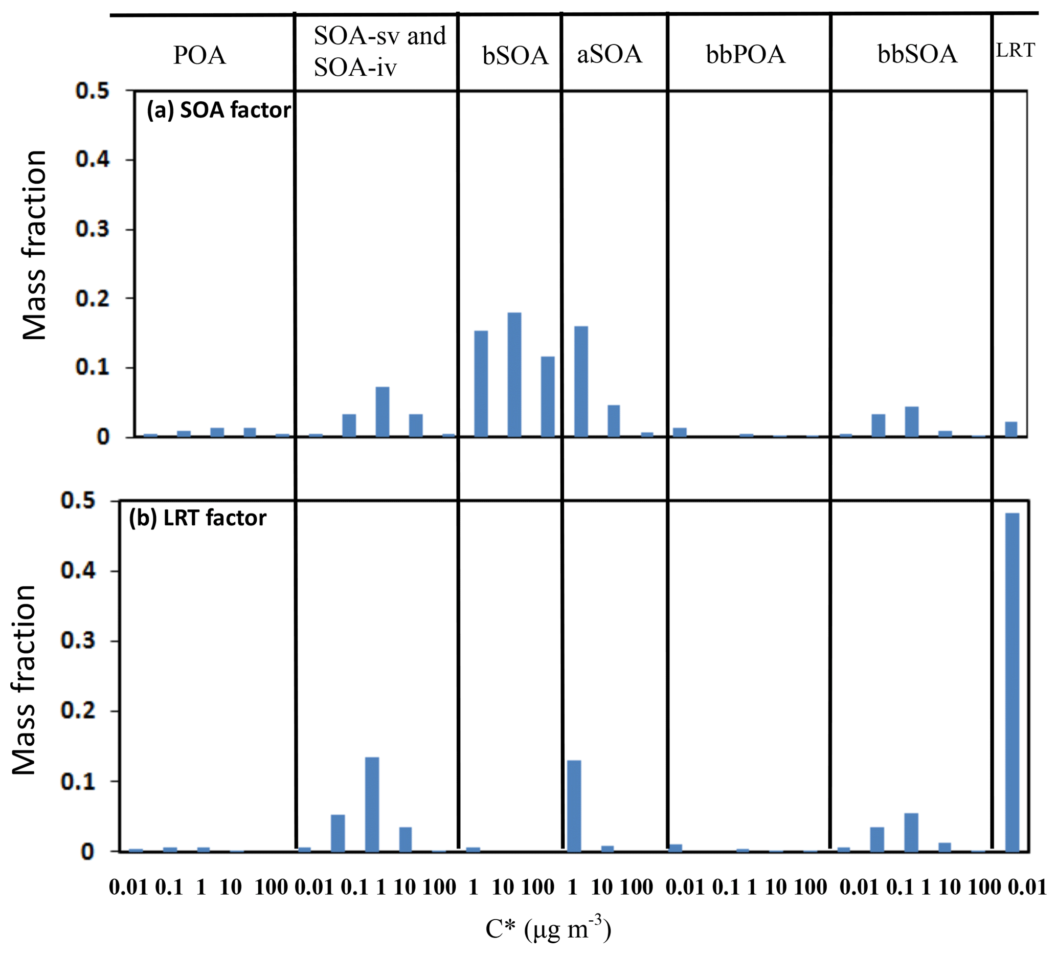
Figure 1Factor profiles resulting from the PMF analysis of the PMCAMx-SR OA predictions in Melpitz: (a) SOA factor and (b) LRT factor.
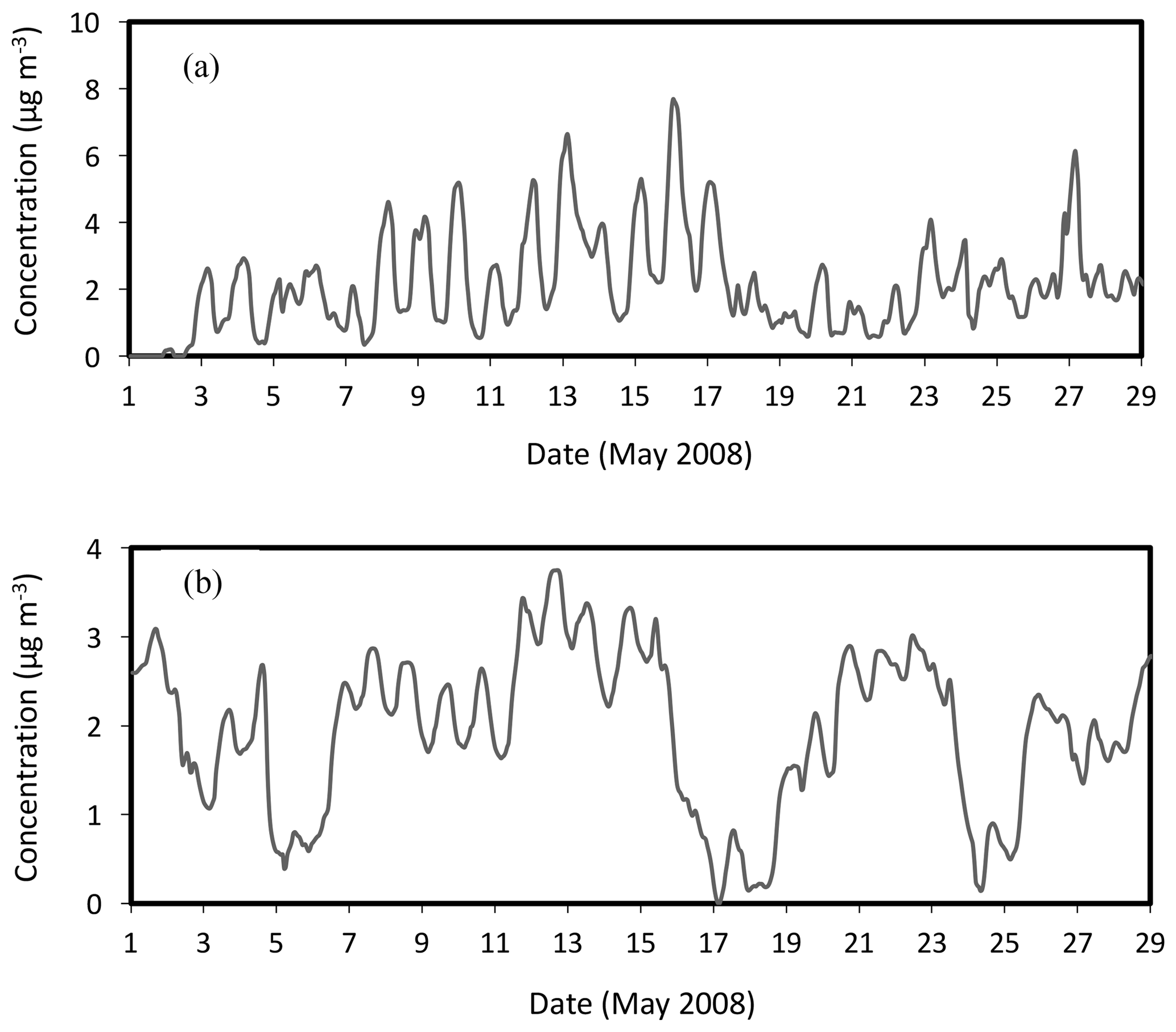
Figure 2PMCAMx-SR factor time series of the (a) SOA and (b) LRT factors in Melpitz during May 2008.
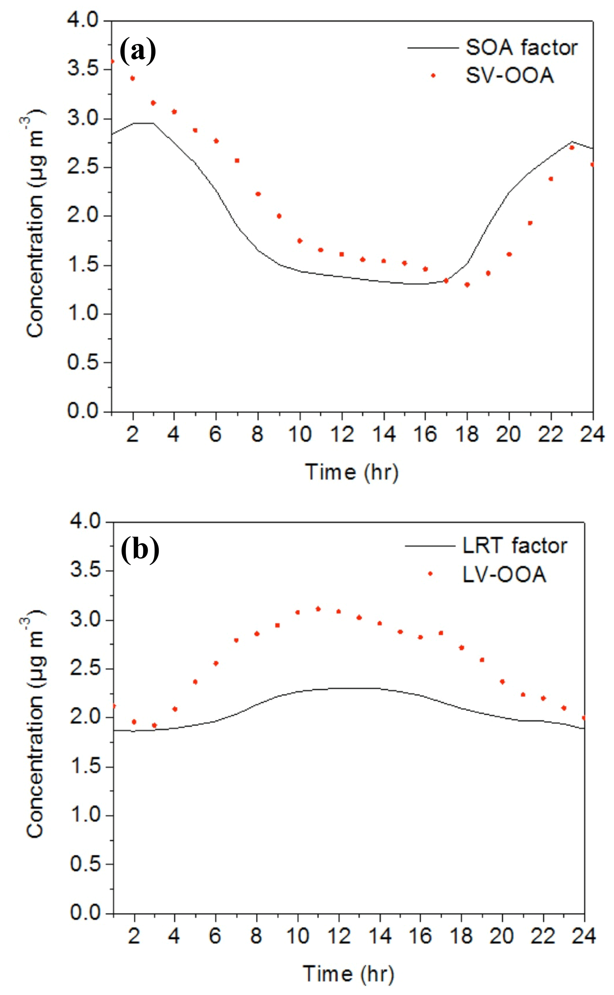
Figure 3Comparison of average diurnal profiles of factors of PMF analysis of PMCAMx-SR results and PMF analysis of AMS measurements in Melpitz: (a) SOA factor and SV-OOA and (b) LRT factor and LV-OOA.
During the same period two factors were identified by analyzing the AMS measurements in Melpitz: low-volatility oxygenated OA (LV-OOA) and a semivolatile oxygenated OA (SV-OOA) factor (Poulain et al., 2014). The average diurnal profile of the PMCAMx-SR SOA factor follows the same pattern as SV-OOA (Fig. 3a) with higher values during the night. The PMCAMx-SR LRT factor is less than the AMS LV-OOA factor during the day. These differences can be due to model errors or can be actual differences in the PMF analysis of the two datasets.
The above results are quite encouraging. This analysis of the two datasets suggests that the PMCAMx-SR PMF analysis provides results that are similar to the corresponding analysis of the AMS measurements. Both approaches result in two oxygenated OA factors. The AMS LV-OOA factor appears to correspond even more to the LRT factor of PMCAMx-SR, and the AMS SV-OOA factor to the PMCAMx-SR SOA factor. We will return to the Melpitz dataset in a subsequent section focusing on OOA. In the next two sections we focus on the major primary OA factors.
3.2.1 Biomass burning organic aerosol
In this section, we examine whether the PMCAMx-SR factor which represents biomass burning (bbOA) sources consists of only bbOA components. In St. Petersburg (Russia) PMCAMx-SR predicted that hourly bbOA levels exceeded 200 µg m−3 due to the nearby fires affecting the site on 4–5 May (Fig. S2a). During the full month in this site, the average contribution of fresh biomass burning OA to the total OA was approximately 65 %. During the fire period (4–5 May) the bbOA contribution was 96 %. The four-factor PMF solution seems to best represent the PMCAMx-SR OA predictions in St. Petersburg. PMF determined a factor which consists of 96 % biomass burning POA and low contributions from biogenic SOA and biomass burning SOA components (Fig. 4). This factor will be called the “bbPOA factor”. In this case, the bbPOA factor includes little else. Comparing the time series of the bbPOA factor and the bbPOA predicted by PMCAMx-SR we estimated a fractional error of 5 % and a fractional bias of −3 % (Table S3).

Figure 4Contribution of each OA component to the PMCAMx-SR bbPOA factor in St. Petersburg, Catania, and Majden during May 2008.
In Catania (Italy) the hourly bbPOA concentration exceeded 35 µg m−3 during 15–17 May due to nearby fires (Fig. S2b). During the fire period, the contribution of bbPOA to OA reached 94 %. During the full month, the average bbPOA contribution to the total OA was 40 %. A three-factor PMF solution was selected in this case. PMF determined a factor with 93 % biomass burning POA and the remaining 7 % was biomass burning SOA (4 %), biogenic SOA (2 %), and anthropogenic SOA (1 %) (Fig. 4). The corresponding normalized error when the time series of the bbOA factor was compared to the PMCAMx-SR bbOA predictions was 11 % in this case.
In Majden (FYROM) fires contributed up to 15 µg m−3 of bbPOA on 25–26 May and bbPOA was 75 % of the OA during the fire period (Fig. S2c). The average bbPOA contribution to OA was 14 % during the simulation period. The three-factor PMF solution best fit our data. PMF identified a factor consisting of 81 % bbPOA, 11 % biogenic SOA, 4 % long-range-transported OA, 2 % biomass burning SOA, and 2 % anthropogenic SOA (Fig. 4). The corresponding normalized error comparing this factor against the actual bbPOA was 24 % due to the mixing of the fresh bbPOA with secondary OA from other sources by the PMF.
In Cabauw (the Netherlands) bbPOA contributed 8 % to OA according to PMCAMx-SR, with an average concentration of 0.4 µg m−3. There were no major fires nearby and the predicted hourly bbPOA concentration was always less than 3 µg m−3. The bbPOA in this case was included by the PMCAMx-SR PMF in a “bbPOA∕SOA” factor. This factor is called bbPOA∕SOA because it consisted of bbPOA and SOA components. The PMF analysis did not give a bbPOA factor even when five factors were used. The same lack of a bbPOA factor was found in the analysis of the PMCAMx-SR OA in Melpitz and Finokalia. The maximum predicted hourly concentration of bbPOA in Melpitz was 0.5 µg m−3 and in Finokalia was 0.1 µg m−3. The bbPOA in these areas was less than 2 % of the OA.
In areas affected by major fires (St. Petersburg, Catania, and Majden) the maximum predicted hourly concentration of bbSOA was 12, 6.5, and 5.7 µg m−3, respectively. In all areas examined in this study bbSOA was included mainly in one of the OOA factors, which will be discussed in detail in the next section. This is due to the fact that the temporal evolution of bbSOA is closer to that of the other SOA components. Therefore, the contribution of biomass burning determined by PMF represents a lower estimate of the impact of fires on OA in a receptor since it includes only a small fraction of the bbSOA.
3.2.2 Primary organic aerosol
The ability of PMF to identify the fresh POA from sources other than biomass burning is explored in this section. POA according to PMCAMx-SR contributed 10 % to OA during May in St. Petersburg. The four-factor PMF solution included a factor which consisted of 67 % POA (Fig. 5). The remaining was SOA-sv and SOA-iv (9 %), biogenic SOA (6 %), anthropogenic SOA (5 %), biomass burning POA (8 %), and biomass burning SOA (5 %). We call this the “POA factor”, but it clearly includes other OA components. For the purposes of our analysis, we consider that PMF identifies a POA factor if there is a factor containing more than 60 % POA. The POA factor and PMCAMx-SR POA concentrations correlated well to each other (R2=0.99, Fig. S3). The average concentration of the POA factor was 1.1 µg m−3 and that of the actual POA was 0.9 µg m−3. The normalized error of the POA factor compared to the PMCAMx-SR POA was 34 % (Table S4).
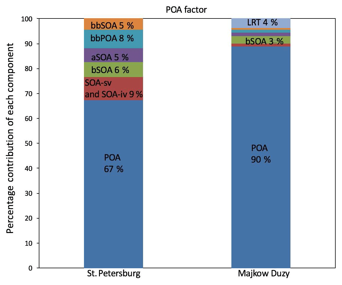
Figure 5Contribution of each OA component to the PMCAMx-SR PMF POA factor in St. Petersburg (Russia) and Majkow Duzy (Poland) during May 2008.
The highest contribution of POA to total OA was predicted in Majkow Duzy in central Poland and it was 50 %. In this location, the POA contributed 90 % to the corresponding POA factor (Fig. 5). The remaining was biogenic SOA (3 %), long-range-transported OA (4 %), anthropogenic SOA (1 %), biogenic SOA (1 %), and biomass burning SOA (1 %). The average concentration of the POA factor was 3.2 µg m−3, while the actual PMCAMx-SR POA was 3.4 µg m−3. The normalized error of the POA factor 10 % in this case (Table S4).
In rural and remote sites (Cabauw, Melpitz, and Finokalia) POA contributed around 3 % to the total OA according to PMCAMx-SR. In Cabauw the three-factor solution included factors which contained 6 %, 11 %, and 10 % POA, respectively. In the four-factor solution POA contributed 12 %, 10 %, 5 %, and 0 % to the factors. In these areas, PMF did not separate the POA from the rest of the OA components.
3.3 PMF source apportionment error for primary OA components
The above analysis of the bbOA and POA factors suggests that the corresponding PMF error does depend on the magnitude of the contribution of the corresponding source to the total OA levels. Higher relative errors are estimated when a source contributes less to the total OA. To better quantify the corresponding dependence of the error on the magnitude of the source we used the PMF solutions in a number of locations and we also artificially scaled up and down the predicted bbOA and POA in certain locations (St. Petersburg, Maiden, Catania, Cabauw, and Majkow Duzy) and repeated the PMF analysis. The results are summarized in Fig. 6.
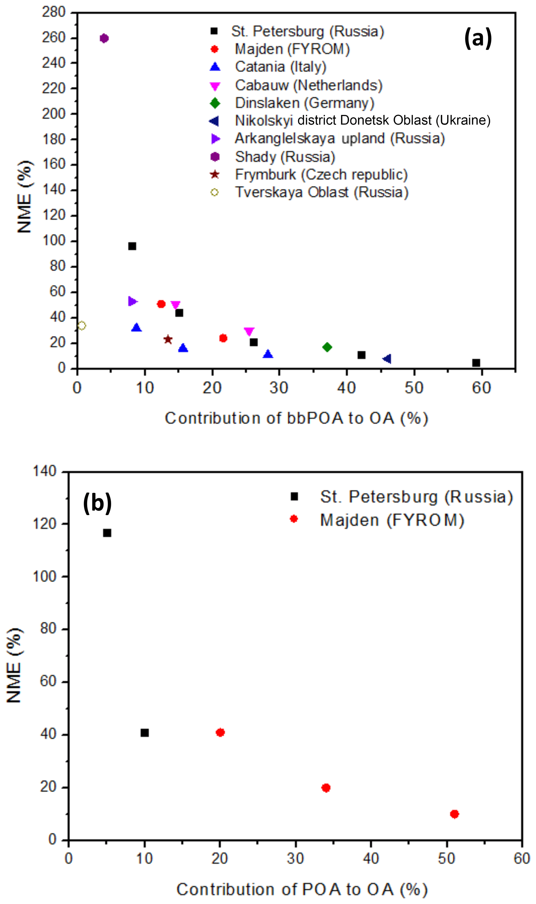
Figure 6PMF normalized error (%) for (α) bbPOA and (β) POA for various locations as a function of their contribution to OA.
The normalized mean error of the bbPOA estimated by the PMF is less than 30 % when the bbPOA contributes more than 20 % to the total OA in the area. The error is reduced to less than 20 % for contributions higher than 30 %. On the other hand, when the bbPOA represents 10 %–20 % of the total OA the PMF error can be up to 50 %. When biomass burning contributes less than 10 % the error is 200 %–300 %. Please note that in these cases, the absolute error is still reasonable and the PMF correctly predicts that bbOA is a relatively small component of OA.
The uncertainty in POA from other sources appears to be a little higher than that of bbPOA probably because PMF mixes it with other sources that have similar temporal profiles. When the POA represents more than 20 % of the OA, the PMF error is less than 40 %. The errors can be up to a factor of 2, when the POA is less than 20 % of the OA.
3.4 Oxygenated organic aerosol
In this section we try to determine the characteristics that differentiate the two OOA factors that are often present in ambient AMS data analysis. One hypothesis is that the two OOA factors contain different OA components (e.g., anthropogenic versus biogenic). A second hypothesis is that one represents the semivolatile and the other the low-volatility OA components. The third hypothesis is that these two factors have different degrees of aging (one is relatively fresh SOA and the other SOA that has undergone multiple generations of oxidation).
The two PMCAMx-SR OOA factors in all areas consist mainly of multiple SOA components. The first OOA factor determined by PMF analysis of PMCAMx-SR OA predictions contains mainly OA from long-range transport. This factor was determined in all areas examined.
In St. Petersburg long-range-transported OA was 11 % of the OA according to PMCAMx-SR. The four-factor solution included a factor which contained 55 % long-range-transported OA and is described here as the “LRT factor” (Fig. 7). In Majden the contribution of long-range-transported OA to total OA was 25 %. In this area PMF determined a LRT factor with 68 % long-range-transported OA. In Catania long-range-transported OA contributed 29 % to OA and the LRT factor consists of 70 % long-range-transported OA. In Cabauw and Melpitz the contribution of long-range-transported OA was 21 % and 24 % and the corresponding LRT factors consist of 58 % and 48 % long-range-transported OA, respectively. During May, the highest contribution of long-range-transported OA to total OA was determined in Finokalia and it was around 40 %. In this site, the long-range-transported OA contributed 87 % to the LRT factor (Fig. 7). Thus, the contribution of highly aged OA transported from outside the domain to the LRT factor ranges from approximately 50 % to 90 % for the areas examined.
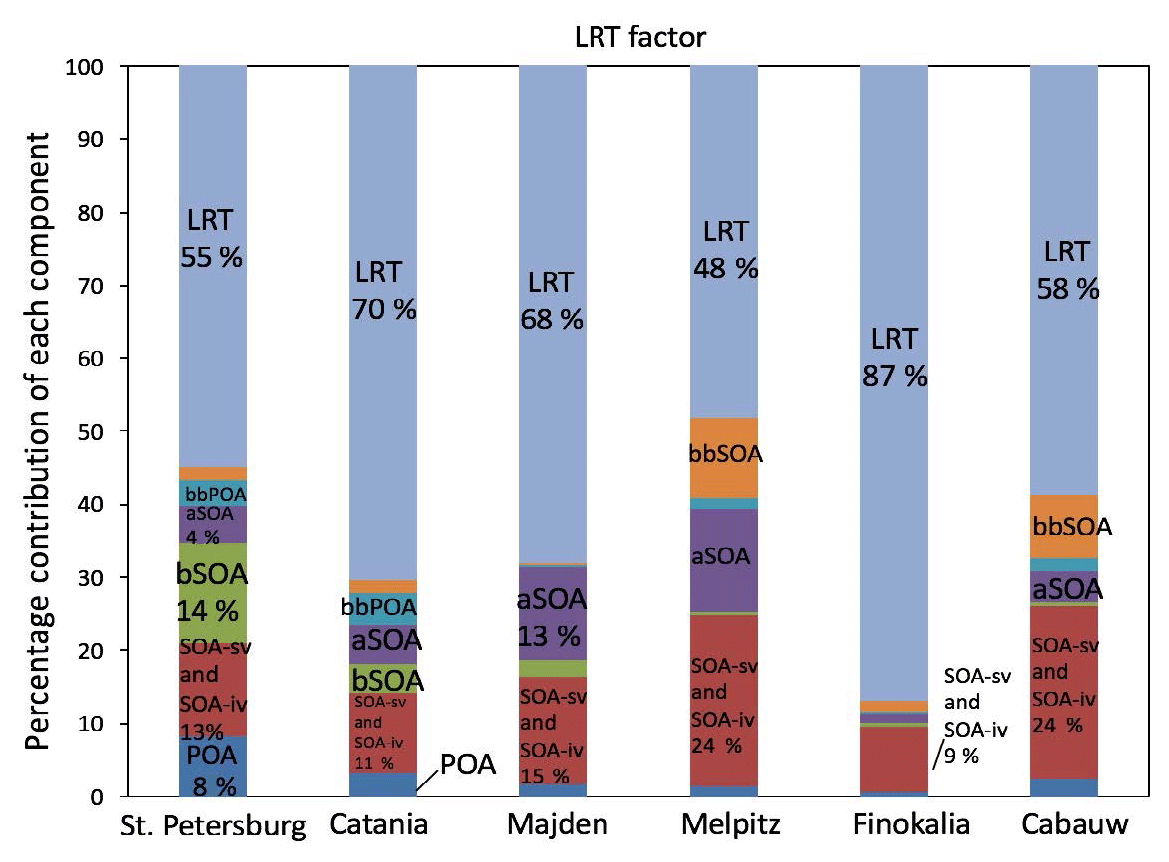
Figure 7Contribution of each OA component to the PMCAMx-SR LRT factor in St. Petersburg, Catania, Majden, Melpitz, and Finokalia during May 2008.
The second OOA factor determined in all areas contains SOA-sv and SOA-iv, anthropogenic SOA, biomass burning SOA, and biogenic SOA (Fig. 8). We call this the “SOA factor” because it mostly includes SOA produced inside the modeling domain. In Catania, PMF combines bbSOA (20 % contribution to SOA factor), aSOA (20 %), and SOA-sv and SOA-iv (30 %) in the SOA factor because the time series of these OA components follow a similar pattern during the simulation period (Fig. S4). This is also the case in the other areas (Majden, Melpitz, and Finokalia; Figs. S5–S7) examined. The contribution of each SOA component to the SOA factor depends on the examined area. Therefore, the SOA factor consists of a mixture of contributions from various anthropogenic and biogenic sources.
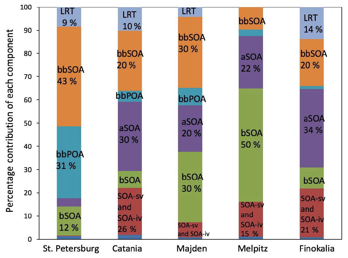
Figure 8Contribution of each OA component to the PMCAMx-SR SOA factor in St. Petersburg, Catania, Majden, Melpitz, and Finokalia during May 2008.
While the two OOA factors both include a mixture of all SOA components (Figs. 8 and 9) the LRT factor is dominated by the highly aged OA transported to Europe from outside the domain, while the SOA factor includes mainly SOA produced over Europe. Therefore, the hypothesis that PMF separates the SOA components based on their sources (e.g., biogenic versus anthropogenic) is not supported by our results.
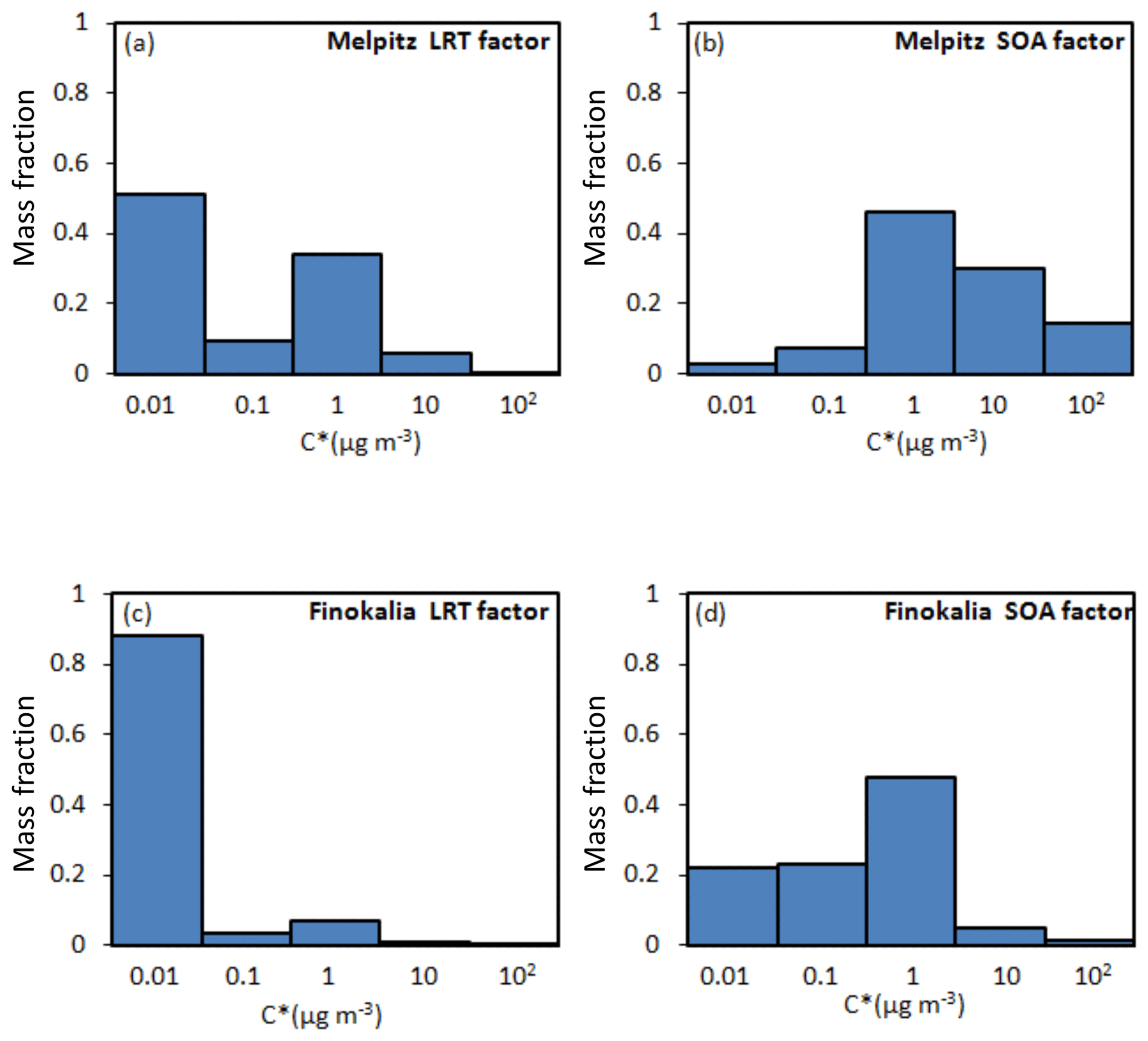
Figure 9Volatility distribution of the (a) LRT factor in Melpitz, (b) SOA factor in Melpitz, (c) LRT factor in Finokalia, and (d) SOA factor in Finokalia.
3.4.1 Volatility of OOA factors
We analyzed the volatility distribution of the two PMCAMx-SR OOA factors predicted by PMCAMx-SR in order to examine whether these factors include OA components with different volatility. In Melpitz the volatility distribution of the SOA factor peaks at effective saturation concentration equal to 1 µg m−3 (Fig. 9a). A total of 90 % of the OA in this factor has effective saturation concentration (C*) higher than or equal to 1 µg m−3. On the other hand, the LRT factor is dominated by components with C* equal to 0.01 and 0.1 µg m−3, contributing 80 % to the factor. In Finokalia the highest mass fraction of the LRT factor has effective saturation concentration equal to 0.01 µg m−3 (Fig. 9c). The LRT factor in this case contains almost exclusively low-volatility OA. The SOA factor includes both low-volatility and semivolatile components. In St. Petersburg, Catania, and Majden the results for the volatility distribution of LRT and SOA factor were between those in St. Petersburg and in Finokalia (Fig. S8).
These results suggest that both factors have components covering a wide range of volatilities and their volatility distributions overlap. However, the LRT factor has on average lower volatility than the SOA factor. These suggest that the PMF does not separate these factors exclusively based on the volatility of the corresponding components. For example, in Melpitz both factors include a lot of OA with C* equal to 1 µg m−3.
The use of the volatility-based terminology (low-volatility and semivolatile OOA) suggests that there is a volatility threshold and OA components that are more volatile than this are grouped by PMF in one factor (e.g., SV-OOA) and the less volatile compounds in the second (LV-OOA). Our results both from this theoretical analysis but also from direct volatility measurements of AMS factors (Paciga et al., 2016; Louvaris et al., 2017) show that this is not the case. The so-called semivolatile factor may include very low-volatility OA, and vice versa, the so-called low-volatility factor may include semivolatile material.
3.4.2 The degree of aging of OOA factors
We applied PMF analysis to PSAT results, separating all the SOA components into two subcategories, first generation and later generation products (second, third, etc.), to investigate whether the degree of chemical processing differentiates the two OOA factors.
In Melpitz the first PMCAMx∕PSAT factor consists of 63 % first generation OA and 37 % later generation OA and is called the “less aged factor” (Fig. 10). The second factor includes 97 % later generation OA and can be described as the “more aged factor”.
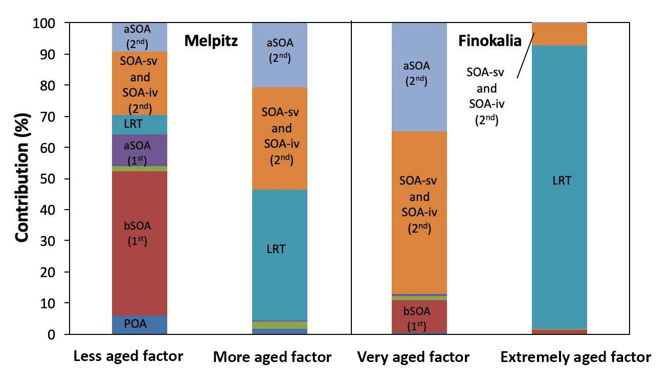
Figure 10Contribution of first generation and second plus later generations of SOA components to each factor in Melpitz and Finokalia during May 2008.
In the more remote site of Finokalia, we determined two factors which both contain aged OA. We characterize the first factor as “extremely aged” because highly aged long-range-transported OA dominated this factor (98 %) (Fig. 10). The second factor is characterized as “very aged”, containing 32 % later generation aSOA, 54 % later generation SOA from semivolatile and intermediate volatility organic compounds and only 14 % first generation SOA. These results are consistent with the analysis of Hildebrandt et al. (2010) who argued that the OA behavior in Finokalia is quite different to that in continental European sites and that the two OOA factors are quite similar to each other. This is also predicted by PMCAMx-SR, suggesting that the model is consistent with that interpretation of the measurements.
One of the limitations of this application of PMCAMx-SR is that we assumed constant low-volatility OA boundary conditions. In general boundary conditions of regional chemical transport models are obtained from the output of similar global models or from some averages of measurements and can be a lot more variable (both in concentration but also in composition and volatility). Obviously, the absolute OA concentrations, especially near the boundaries of the domain, can be dominated by these boundary conditions. To avoid such issues, in this analysis we have used sites that are far from the boundaries. Overall, our conclusions are quite robust to the choice of the OA boundary condition values.
Our analysis suggests that the evolution of the terms used to describe the often-observed two OOA factors reflects our understanding (or lack thereof) of the nature of these factors and not so much site-to-site variability. The use of OOA-1 and OOA-2 reflected the complete lack of understanding. Then the use of less and more volatile OOA showed the beginning of some understanding, but it has probably led to some confusion and a few misconceptions. The next step (use of less and more oxidized OA) is probably more accurate. Our work here supports the hypothesis that these factors correspond to less and more aged OOA present in each site.
3.4.3 Comparison of OOA factors of PMF and ME-2 analysis
In this section, we compare the two OOA factors determined by PMF and ME-2 analysis in order to estimate the change in these factors when ME-2 analysis is used. In ME-2 we used the “correct” POA factor (forced the model to assume 100 % contribution of POA to the POA factor). Moving from PMF to ME-2, the changes in the composition of the SOA and LRT factor were minor in all examined areas. Figures S9 and S10 illustrate the two OOA factors in Melpitz and in Finokalia when PMF and ME-2 are used. Thus, the above conclusions for the two OOA factors do not change when ME-2 is used. The advantage of the use of ME-2 analysis is that a better separation of primary sources is obtained if of course the correct POA fingerprint is used.
3.5 Sensitivity analysis
To better quantify the role of the volatility of the OA components on the results of the PMF analysis we repeated the PMF application on the PMCAMx-SR predictions, this time using only the volatility distributions of the predicted total OA as inputs. In this case the PMF inputs were the total concentrations of OA in the five C* volatility bins ranging from 10−2 to 102 µg m−3. We first assumed two factors. The resulting PMF factors included material from all volatility bins. For example, for St. Petersburg, the first factor contained 65 % semivolatile OA and the second contained 70 %, with the rest being low-volatility OA. So PMF did not separate the OA into semivolatile and low-volatility material. In the next step we assumed three factors, but still the factors included surrogate compounds with a mixture of volatilities. These results suggest once more that the OA volatility plays a secondary role in the process in which PMF separates the OA components into factors.
In a second test, we performed PMF analysis on a dataset consisting of the PMCAMx-SR hourly predictions for six of the sites (St. Petersburg, Catania, Majden, Melpitz, Finokalia, and Cabauw) used in the analysis in the previous sections. Something like this is rarely done with field data because it is assumed that the composition of the primary and secondary factors may be different in different areas. Thus, the merging of the datasets may introduce additional uncertainties in the PMF analysis. In this case, the composition of all sources in all areas is assumed to be the same in PMCAMx-SR, so one can examine the behavior of PMF in this ideal situation. PMF could reproduce the overall dataset using four factors: a primary OA factor, a biomass burning OA factor, and two secondary OA factors.
For the primary OA factors, applying PMF to the complete dataset resulted in factor compositions that had an intermediate composition compared to the factors from the site-by-site analysis. For example, the POA factor in the common analysis contained 81 % fresh POA, a value close to the middle of the 67 % for St. Petersburg and the 89 % for Majkow Duzy (Fig. S11). The predicted concentrations of the POA factor in the site-by-site and common PMF were quite similar, with differences less than 10 % in the average predicted concentrations (Fig. S12). The same behavior was observed for primary bbOA, with the common analysis giving intermediate results but closer to the best than the average. The corresponding PMF bbOA factor contained 93 % bbOA in this case (Fig. S13), a little less than the 96 % in the independent analysis of the St. Petersburg predictions, but a lot more than the 81 % in Majden. The bbOA factor time series for the site-by-site analysis were once more quite similar to each other (Fig. S14), with differences in the average concentrations of less than 15 %.
The situation was quite different for the OOA factors. The results of the common analysis were quite different from those of the site-by-site analysis in most but not all sites. For example, the common SOA factor contained 27 % biogenic SOA, while the corresponding factors for the site-by-site analysis contained from approximately 5 % to 42 % bSOA (Fig. S15). It is interesting, though, that the common SOA factor did not include any aged OA from long-range transport. The resulting concentrations of the predicted SOA factor for the common analysis could be quite different from those of the site-by-site analysis. For example, in St. Petersburg the concentration of the SOA factor was 1.1 µg m−3 for the site-by-site analysis and 0.7 µg m−3 for the common analysis (Fig. S16). On the other hand, for Catania the results of the approaches were quite similar, with average concentrations of 1.5 µg m−3 for the site-by-site and 1.3 µg m−3 for the common analysis (Fig. S17). The common LRT factor contained 73 % OA from long-range transport a value closer to the upper limit (79 % for Finokalia) than to the lower (47 % for Melpitz) for the site-by-site analysis (Fig. S18). The average concentration of the LRT factor in Melpitz was 1.9 µg m−3 for the individual and 1.3 µg m−3 for the common analysis (Fig. S19). These results indicate that the composition of the OOA factors and the resulting concentrations are quite sensitive to the range of data included in the analysis.
We analyzed for the first time, to the best of our knowledge, the organic aerosol composition predictions of a chemical transport model (PMCAMx-SR) using positive matrix factorization in an effort to better understand the results of PMF analysis of ambient organic aerosol AMS measurements. The high-level results of our analysis are quite consistent with those of the corresponding field studies; we find similar quantities and characteristics of factors for a number of sites in Europe. This consistency indicates that the analysis of the model results can be used as a first-order interpretation of the various factors often reported in field data PMF analysis. These factors include the hydrocarbon-like OA and biomass burning OA and two oxygenated organic OA factors. Cooking OA was not included as a source in the emissions inventory used, so it cannot be studied at this stage.
The primary OA factor (which corresponds to the hydrocarbon-like OA in AMS analysis) of the PMCAMx-SR predictions usually contains not only primary OA compounds but also secondary components or biomass burning OA. These additional components represent on average one-third of the factor mass. The average error of using HOA instead of POA is around 25 % in the cases examined and increases when the POA contribution to OA decreases. PMF identifies a POA factor in the PMCAMx-SR predictions when this group of sources contributes more than 10 % to the OA and is one of the top three sources.
PMF determines a biomass burning OA factor in all areas influenced by major nearby fires. In these cases of major fire influence, the biomass burning primary OA factor consists of around 90 % biomass burning primary OA. The error in the bbPOA factor is less than 30 %, when biomass burning contributes more than 20 % to the average OA. The biomass burning secondary OA is always grouped with secondary OA components and only a small fraction of it is included in the biomass burning factor. Therefore, the bbOA factor provides a lower limit of the impact of fires on the OA of an area.
Our analysis suggests that PMF has difficulties identifying sources that contribute approximately 10 % or less to the total OA during the period of the analysis. The use of ME-2 constraining the primary OA factor (which contains 100 % contribution from primary OA) provides a better separation of primary and secondary sources, reducing the contribution of POA to the two oxygenated OA factors. However, this assumes perfect knowledge of the “fingerprint” of the POA factor.
The two oxygenated OA factors both contain a series of SOA components from both anthropogenic and biogenic sources. The first oxygenated OA factor includes mainly highly aged OA transported from outside Europe, but also highly aged secondary OA from sources in Europe that has undergone multiple generations of oxidation. The second oxygenated OA factor contains SOA from volatile, semivolatile, and intermediate volatility anthropogenic and biogenic organic compounds. The exact contribution of these OA components to each OA factor depends on the site. In rural continental areas (like Melpitz) the first oxygenated OA factor includes highly aged secondary OA and the second includes mostly “fresh” first-generation secondary organic compounds. On the other hand, in remote sites such as in Finokalia in Crete, both oxygenated OA factors include organic components that have undergone two or more generations of aging. This suggests that the PMF determines the two extremes of the chemical processing of the OA present in the site during the measurements and reports them as the corresponding OOA factors.
Most of the time, the two oxygenated OA factors have overlapping volatility distributions and therefore their characterization as low and high volatility that has been used in the literature may be misleading in at least some cases. This is consistent with the measurements of Paciga et al. (2016) in Paris and Louvaris et al. (2017) in Athens. However, the more aged factor has lower average volatility than the fresh secondary OA factor.
Our results suggest that the comparison of CTM predictions of POA and fresh biomass burning OA to the corresponding AMS results is meaningful if these are major sources for the specific locations. The PMF uncertainties estimated here should also be taken into account. The comparison of the less and more volatile OA predicted by CTMs to the corresponding OOA factors is probably not a good idea. Summation of the two OOA factors into just OOA appears to be quite safe, based on our results here. On the other hand, if a CTM can keep track of the age of OA the comparison of more and less aged predicted OA to the two OOA factors could be potentially useful.
The data in the study are available from the authors upon request (spyros@chemeng.upatras.gr).
The supplement related to this article is available online at: https://doi.org/10.5194/acp-19-973-2019-supplement.
ADD conducted the simulations, analysed the results, and wrote the paper. KS assisted in the PSAT implementation and the analysis of the chemical aging results. GNT contributed to the analysis of the PMCAMx-SR results. SNP was responsible for the design and coordination of the study and the synthesis of the results.
The authors declare that they have no conflict of interest.
This work has been supported by the US Environmental Protection Agency (EPA)
Center for Air, Climate and Energy Solutions (CACES) (grant number R835873).
The authors would like to thank Kalliopi Florou for her assistance with PMF.
Edited by: Lynn M. Russell
Reviewed by: two anonymous referees
Aiken, A. C., Salcedo, D., Cubison, M. J., Huffman, J. A., DeCarlo, P. F., Ulbrich, I. M., Docherty, K. S., Sueper, D., Kimmel, J. R., Worsnop, D. R., Trimborn, A., Northway, M., Stone, E. A., Schauer, J. J., Volkamer, R. M., Fortner, E., de Foy, B., Wang, J., Laskin, A., Shutthanandan, V., Zheng, J., Zhang, R., Gaffney, J., Marley, N. A., Paredes-Miranda, G., Arnott, W. P., Molina, L. T., Sosa, G., and Jimenez, J. L.: Mexico City aerosol analysis during MILAGRO using high resolution aerosol mass spectrometry at the urban supersite (T0) – Part 1: Fine particle composition and organic source apportionment, Atmos. Chem. Phys., 9, 6633–6653, https://doi.org/10.5194/acp-9-6633-2009, 2009.
Allan, J. D., Williams, P. I., Morgan, W. T., Martin, C. L., Flynn, M. J., Lee, J., Nemitz, E., Phillips, G. J., Gallagher, M. W., and Coe, H.: Contributions from transport, solid fuel burning and cooking to primary organic aerosols in two UK cities, Atmos. Chem. Phys., 10, 647–668, https://doi.org/10.5194/acp-10-647-2010, 2010.
Brinkman, G., Vance, G., Hannigan, M. P., and Milford, J. B.: Use of synthetic data to evaluate positive matrix factorization as a source apportionment tool for PM2.5 exposure data, Environ. Sci. Technol., 40, 1892–1901, 2006.
Canonaco, F., Crippa, M., Slowik, J. G., Baltensperger, U., and Prévôt, A. S. H.: SoFi, an IGOR-based interface for the efficient use of the generalized multilinear engine (ME-2) for the source apportionment: ME-2 application to aerosol mass spectrometer data, Atmos. Meas. Tech., 6, 3649–3661, https://doi.org/10.5194/amt-6-3649-2013, 2013.
Dall'Osto, M., Paglione, M., Decesari, S., Facchini, M. C., O'Dowd, C., Plass-Duellmer, C., and Harrison, R. M.: On the origin of AMS cooking Organic Aerosol at a rural site, Environ. Sci. Technol., 49, 13964–13972, 2015.
de Gouw, J. and Jimenez, J. L.: Organic aerosols in the earth's atmosphere, Environ. Sci. Technol., 43, 7614–7618, 2009.
Donahue, N. M., Robinson, A. L., Stanier, C. O., and Pandis, S. N.: Coupled partitioning, dilution, and chemical aging of semivolatile organics, Environ. Sci. Technol., 40, 2635–2643, 2006.
Fountoukis, C., Racherla, P. N., Denier van der Gon, H. A. C., Polymeneas, P., Charalampidis, P. E., Pilinis, C., Wiedensohler, A., Dall'Osto, M., O'Dowd, C., and Pandis, S. N.: Evaluation of a three-dimensional chemical transport model (PMCAMx) in the European domain during the EUCAARI May 2008 campaign, Atmos. Chem. Phys., 11, 10331–10347, https://doi.org/10.5194/acp-11-10331-2011, 2011.
Fountoukis, C., Megaritis, A. G., Skyllakou, K., Charalampidis, P. E., Pilinis, C., Denier van der Gon, H. A. C., Crippa, M., Canonaco, F., Mohr, C., Prévôt, A. S. H., Allan, J. D., Poulain, L., Petäjä, T., Tiitta, P., Carbone, S., Kiendler-Scharr, A., Nemitz, E., O'Dowd, C., Swietlicki, E., and Pandis, S. N.: Organic aerosol concentration and composition over Europe: insights from comparison of regional model predictions with aerosol mass spectrometer factor analysis, Atmos. Chem. Phys., 14, 9061–9076, https://doi.org/10.5194/acp-14-9061-2014, 2014.
Hildebrandt, L., Donahue, N. M., and Pandis, S. N.: High formation of secondary organic aerosol from the photo-oxidation of toluene, Atmos. Chem. Phys., 9, 2973–2986, https://doi.org/10.5194/acp-9-2973-2009, 2009.
Hildebrandt, L., Engelhart, G. J., Mohr, C., Kostenidou, E., Lanz, V. A., Bougiatioti, A., DeCarlo, P. F., Prevot, A. S. H., Baltensperger, U., Mihalopoulos, N., Donahue, N. M., and Pandis, S. N.: Aged organic aerosol in the Eastern Mediterranean: the Finokalia Aerosol Measurement Experiment – 2008, Atmos. Chem. Phys., 10, 4167–4186, https://doi.org/10.5194/acp-10-4167-2010, 2010.
Hodzic, A., Jimenez, J. L., Madronich, S., Canagaratna, M. R., DeCarlo, P. F., Kleinman, L., and Fast, J.: Modeling organic aerosols in a megacity: potential contribution of semi-volatile and intermediate volatility primary organic compounds to secondary organic aerosol formation, Atmos. Chem. Phys., 10, 5491–5514, https://doi.org/10.5194/acp-10-5491-2010, 2010.
Huffman, J. A., Docherty, K. S., Aiken, A. C., Cubison, M. J., Ulbrich, I. M., DeCarlo, P. F., Sueper, D., Jayne, J. T., Worsnop, D. R., Ziemann, P. J., and Jimenez, J. L.: Chemically-resolved aerosol volatility measurements from two megacity field studies, Atmos. Chem. Phys., 9, 7161–7182, https://doi.org/10.5194/acp-9-7161-2009, 2009.
IPCC (Intergovernmental Panel on Climate Change): Climate Change 2014: Mitigation of Climate Change. Contribution of Working Group III to the Fifth Assessment Report of the Intergovernmental Panel on Climate Change, Cambridge University Press, Cambridge, UK and New York, 2014.
Jimenez, J. L., Canagaratna, M. R., Donahue, N. M., Prevot, A. S. H., Zhang, Q., Kroll, J. H., DeCarlo, P. F., Allan, J. D., Coe, H., Ng, N. L., Aiken, A. C., Docherty, K. S., Ulbrich, I. M., Grieshop, A. P., Robinson, A. L., Duplissy, J., Smith, J. D., Wilson, K. R., Lanz, V. A., Hueglin, C., Sun, Y. L., Tian, J., Laaksonen, A., Raatikainen, T., Rautiainen, J., Vaattovaara, P., Ehn, M., Kulmala, M., Tomlinson, J. M., Collins, D. R., Cubison, M. J., Dunlea, E. J., Huffman, J. A., Onasch, T. B., Alfarra, M. R., Williams, P. I., Bower, K., Kondo, Y., Schneider, J., Drewnick, F., Borrmann, S., Weimer, S., Demerjian, K., Salcedo, D., Cottrell, L., Griffin, R., Takami, A., Miyoshi, T., Hatakeyama, S., Shimono, A., Sun, J. Y., Zhang, Y. M., Dzepina, K., Kimmel, J. R., Sueper, D., Jayne, J. T., Herndon, S. C., Trimborn, A. M., Williams, L. R., Wood, E. C., Middlebrook, A. M., Kolb, C. E., Baltensperger, U., and Worsnop, D. R.: Evolution of organic aerosols in the atmosphere, Science, 326, 1525–1529, 2009.
Kanakidou, M., Seinfeld, J. H., Pandis, S. N., Barnes, I., Dentener, F. J., Facchini, M. C., Van Dingenen, R., Ervens, B., Nenes, A., Nielsen, C. J., Swietlicki, E., Putaud, J. P., Balkanski, Y., Fuzzi, S., Horth, J., Moortgat, G. K., Winterhalter, R., Myhre, C. E. L., Tsigaridis, K., Vignati, E., Stephanou, E. G., and Wilson, J.: Organic aerosol and global climate modelling: a review, Atmos. Chem. Phys., 5, 1053–1123, https://doi.org/10.5194/acp-5-1053-2005, 2005.
Kiendler-Scharr, A., Zhang, Qi, Hohaus, T., Kleist, E., Mensah, A., Mentel, T. F., Spindler, Uerlings, R., Tillmann, R., and Wildt, J.: Aerosol mass spectrometric features of biogenic SOA: observations from a plant chamber and in rural atmospheric environments, Environ. Sci. Technol., 43, 8166–8172, 2009.
Kostenidou, E., Florou, K., Kaltsonoudis, C., Tsiflikiotou, M., Vratolis, S., Eleftheriadis, K., and Pandis, S. N.: Sources and chemical characterization of organic aerosol during the summer in the eastern Mediterranean, Atmos. Chem. Phys., 15, 11355–11371, https://doi.org/10.5194/acp-15-11355-2015, 2015.
Kostenidou, E., Karnezi, E., Hite Jr., J. R., Bougiatioti, A., Cerully, K., Xu, L., Ng, N. L., Nenes, A., and Pandis, S. N.: Organic aerosol in the summertime southeastern United States: components and their link to volatility distribution, oxidation state and hygroscopicity, Atmos. Chem. Phys., 18, 5799–5819, https://doi.org/10.5194/acp-18-5799-2018, 2018.
Lane, T. E., Donahue, N. M., and Pandis, S. N.: Simulating secondary organic aerosol formation using the volatility basis-set approach in a chemical transport model, Atmos. Environ., 42, 7439–7451, 2008.
Lanz, V. A., Alfarra, M. R., Baltensperger, U., Buchmann, B., Hueglin, C., and Prévôt, A. S. H.: Source apportionment of submicron organic aerosols at an urban site by factor analytical modelling of aerosol mass spectra, Atmos. Chem. Phys., 7, 1503–1522, https://doi.org/10.5194/acp-7-1503-2007, 2007.
Lanz, V. A., Alfarra, M. R., Baltensperger, U., Buchmann, B., Hueglin, C., Szidat, S., Wehrli, M. N., Wacker, L., Weimer, S., Caseiro, A., Puxbaum, J., and Prévôt, A. S. H.: Source attribution of submicron organic aerosols during wintertime inversions by advanced factor analysis of aerosol mass spectra, Environ. Sci. Technol., 42, 214–220, 2008.
Louvaris, E. E., Florou, K., Karnezi, E., Papanastasiou, D. K., Gkatzelis, G. I., and Pandis, S. N.: Volatility of source apportioned wintertime organic aerosol in the city of Athens, Atmos. Environ., 158, 138–147, 2017.
May, A. A., Levin, E. J. T., Hennigan, C. J., Riipinen, I., Lee, T., Collett, J. L., Jimenez, J. L., Kreidenweis, S. M., and Robinson, A. L.: Gas-particle partitioning of primary organic aerosol emissions: 3. Biomass burning, J. Geophys. Res., 118, 11327–11338, 2013.
Murphy, B. N. and Pandis, S. N.: Simulating the formation of semivolatile primary and secondary organic aerosol in a regional chemical transport model, Environ. Sci. Technol., 43, 4722–4728, 2009.
Ng, N. L., Kroll, J. H., Keywood, M. D., Bahreini, R., Varutbangkul, V., Flagan, R. C., and Seinfeld, J. H.: Contribution of first- versus second-generation products to secondary organic aerosols formed in the oxidation of biogenic hydrocarbons, Environ. Sci. Technol., 40, 2283–2297, 2006.
Ng, N. L., Canagaratna, M. R., Zhang, Q., Jimenez, J. L., Tian, J., Ulbrich, I. M., Kroll, J. H., Docherty, K. S., Chhabra, P. S., Bahreini, R., Murphy, S. M., Seinfeld, J. H., Hildebrandt, L., Donahue, N. M., DeCarlo, P. F., Lanz, V. A., Prévôt, A. S. H., Dinar, E., Rudich, Y., and Worsnop, D. R.: Organic aerosol components observed in Northern Hemispheric datasets from Aerosol Mass Spectrometry, Atmos. Chem. Phys., 10, 4625–4641, https://doi.org/10.5194/acp-10-4625-2010, 2010.
Paatero, P.: The multilinear engine – A table-driven, least squares program for solving multilinear problems, including the n-way parallel factor analysis model, J. Comput. Graph. Stat., 8, 854– 888, 1999.
Paatero, P. and Tapper, U.: Positive Matrix Factorization: a nonnegative factor model with optimal utilization of error estimates of data values, Environmetrics, 5, 111–126, 1994.
Paciga, A., Karnezi, E., Kostenidou, E., Hildebrandt, L., Psichoudaki, M., Engelhart, G. J., Lee, B.-H., Crippa, M., Prévôt, A. S. H., Baltensperger, U., and Pandis, S. N.: Volatility of organic aerosol and its components in the megacity of Paris, Atmos. Chem. Phys., 16, 2013–2023, https://doi.org/10.5194/acp-16-2013-2016, 2016.
Pope, C. A., Ezzati, M., and Dockery, D. W.: Fine-particulate air pollution and life expectancy in the United States, New Engl. J. Med., 360, 376–386, 2009.
Poulain, L., Birmili, W., Canonaco, F., Crippa, M., Wu, Z. J., Nordmann, S., Spindler, G., Prévôt, A. S. H., Wiedensohler, A., and Herrmann, H.: Chemical mass balance of 300 ∘C non-volatile particles at the tropospheric research site Melpitz, Germany, Atmos. Chem. Phys., 14, 10145–10162, https://doi.org/10.5194/acp-14-10145-2014, 2014.
Robinson, A. L., Donahue, N. M., Shrivastava, M. K., Weitkamp, E. A., Sage, A. M., Grieshop, A. P., Lane, T. E., Pierce, J. R., and Pandis, S. N.: Rethinking organic aerosol: semivolatile emissions and photochemical aging, Science, 315, 1259–1262, 2007.
Seinfeld, J. H. and Pandis, S. N.: Atmospheric Chemistry and Physics, 2nd Edn., John Wiley and Sons, Hoboken, New Jersey, USA, 2006.
Shrivastava, M. K., Lane, T. E., Donahue, N. M., Pandis, S. N., and Robinson, A. L.: Effects of gas-particle partitioning and aging of primary emissions on urban and regional organic aerosol concentrations, J. Geophys. Res., 113, D18301, https://doi.org/10.1029/2007JD009735, 2008.
Skamarock, W. C., Klemp, J. B., Dudhia, J., Gill, D. O., Barker, D. M., Wang, W., and Powers, J. G.: A Description of the Advanced Research WRF Version 2, NCAR Technical Note, available at: http://www.mmm.ucar.edu/wrf/users/docs/arw_v2.pdf (last access: 21 January 2019), 2005.
Skyllakou, K., Murphy, B. N., Megaritis, A. G., Fountoukis, C., and Pandis, S. N.: Contributions of local and regional sources to fine PM in the megacity of Paris, Atmos. Chem. Phys., 14, 2343–2352, https://doi.org/10.5194/acp-14-2343-2014, 2014.
Skyllakou, K., Fountoukis, C., Charalampidis, P., and Pandis, S. N.: Volatility-resolved source apportionment of primary and secondary organic aerosol over Europe, Atmos. Environ., 167, 1–10, 2017.
Sun, Y., Zhang, Q., Macdonald, A. M., Hayden, K., Li, S. M., Liggio, J., Liu, P. S. K., Anlauf, K. G., Leaitch, W. R., Steffen, A., Cubison, M., Worsnop, D. R., van Donkelaar, A., and Martin, R. V.: Size-resolved aerosol chemistry on Whistler Mountain, Canada with a high-resolution aerosol mass spectrometer during INTEX-B, Atmos. Chem. Phys., 9, 3095–3111, https://doi.org/10.5194/acp-9-3095-2009, 2009.
Sun, Y. L., Wang, Z. F., Fu, P. Q., Yang, T., Jiang, Q., Dong, H. B., Li, J., and Jia, J. J.: Aerosol composition, sources and processes during wintertime in Beijing, China, Atmos. Chem. Phys., 13, 4577–4592, https://doi.org/10.5194/acp-13-4577-2013, 2013.
Theodoritsi, G. N. and Pandis, S. N.: Simulation of the chemical evolution of biomass burning organic aerosol, Atmos. Chem. Phys. Discuss., https://doi.org/10.5194/acp-2018-1166, in review, 2018.
Tsimpidi, A. P., Karydis, V. A., Zavala, M., Lei, W., Molina, L., Ulbrich, I. M., Jimenez, J. L., and Pandis, S. N.: Evaluation of the volatility basis-set approach for the simulation of organic aerosol formation in the Mexico City metropolitan area, Atmos. Chem. Phys., 10, 525–546, https://doi.org/10.5194/acp-10-525-2010, 2010.
Tsimpidi, A. P., Karydis, V. A., Pandis, S. N., and Lelieveld, J.: Global combustion sources of organic aerosols: model comparison with 84 AMS factor-analysis data sets, Atmos. Chem. Phys., 16, 8939–8962, https://doi.org/10.5194/acp-16-8939-2016, 2016.
Ulbrich, I. M., Canagaratna, M. R., Zhang, Q., Worsnop, D. R., and Jimenez, J. L.: Interpretation of organic components from Positive Matrix Factorization of aerosol mass spectrometric data, Atmos. Chem. Phys., 9, 2891–2918, https://doi.org/10.5194/acp-9-2891-2009, 2009.
Wagstrom, K. M., Pandis, S. N., Yarwood, G., Wilson, G. M., and Morris, R. E.: Development and application of a computationally efficient particulate matter apportionment algorithm in a three-dimensional chemical transport model, Atmos. Environ., 42, 5650–5659, 2008.
Xu, L., Guo, H., Weber, R. J., and Ng, N. L.: Chemical characterization of water soluble soluble organic aerosol in contrasting rural and urban environments in the Southeastern United States, Environ. Sci. Technol., 51, 78–88, 2017.
Yuan, B., Shao, M., de Gouw, J., Parrish, D. D., Lu, S., Wang, M., Zeng, L., Zhang, Q., Song, Y., Zhang, J., and Hu, M.: Volatile organic compounds (VOCs) in urban air: How chemistry affects the interpretation of positive matrix factorization (PMF) analysis, J. Geophys. Res., 117, 24302, https://doi.org/10.1029/2012JD018236, 2012.
Zhang, Q., Alfarra, M. R., Wornsop, D. R., Allan, J. D., Coe, H., Canagaratna, M., and Jimenez, J. L.: Deconvolution and quantification of hydrocarbon-like and oxygenated organic aerosols based on aerosol mass spectrometry, Environ. Sci. Technol., 39, 4938–4952, 2005a.
Zhang, Q., Worsnop, D. R., Canagaratna, M. R., and Jimenez, J. L.: Hydrocarbon-like and oxygenated organic aerosols in Pittsburgh: insights into sources and processes of organic aerosols, Atmos. Chem. Phys., 5, 3289–3311, https://doi.org/10.5194/acp-5-3289-2005, 2005b.
Zhang, Q., Jimenez, J. L., Canagaratna, M. R., Allan, J. D., Coe, H., Ulbrich, I., Alfarra, M. R., Takami, A., Middlebrook, A. M., Sun, Y. L., Dzepina, K., Dunlea, E., Docherty, K., DeCarlo, P. F., Salcedo, D., Onasch, T., Jayne, J. T., Miyoshi, T., Shimono, A., Hatakeyama, S., Takegawa, N., Kondo, Y., Schneider, J., Drewnick, F., Borrmann, S., Weimer, S., Demerjian, K., Williams, P., Bower, K., Bahreini, R., Cottrell, L., Griffin, R. J., Rautiainen, J., Sun, J. Y., Zhang, Y. M., and Worsnop, D. R.: Ubiquity and dominance of oxygenated species in organic aerosols in anthropogenically-influenced Northern Hemisphere midlatitudes, Geophys. Res. Lett., 34, L13801, https://doi.org/10.1029/2007GL029979, 2007.
Zhang, Q., Jimenez, J. L., Canagaratna, M. R., Ulbrich, I. M., Ng, N. L., Worsnop, D. R., and Sun, Y.: Understanding atmospheric organic aerosols via factor analysis of aerosol mass spectrometry: a review, Anal. Bioanal. Chem., 401, 3045–3067, 2011.