the Creative Commons Attribution 4.0 License.
the Creative Commons Attribution 4.0 License.
 | 22 Jul 2019
Towards monitoring localized CO2 emissions from space: co-located regional CO2 and NO2 enhancements observed by the OCO-2 and S5P satellites
Maximilian Reuter
Michael Buchwitz
Oliver Schneising
Sven Krautwurst
Christopher W. O'Dell
Andreas Richter
Heinrich Bovensmann
John P. Burrows
Despite its key role in climate change, large uncertainties persist in our knowledge of the anthropogenic emissions of carbon dioxide (CO2) and no global observing system exists that allows us to monitor emissions from localized CO2 sources with sufficient accuracy. The Orbiting Carbon Observatory-2 (OCO-2) satellite allows retrievals of the column-average dry-air mole fractions of CO2 (XCO2). However, regional column-average enhancements of individual point sources are usually small, compared to the background concentration and its natural variability, and often not much larger than the satellite's measurement noise. This makes the unambiguous identification and quantification of anthropogenic emission plume signals challenging. NO2 is co-emitted with CO2 when fossil fuels are combusted at high temperatures. It has a short lifetime on the order of hours so that NO2 columns often greatly exceed background and noise levels of modern satellite sensors near sources, which makes it a suitable tracer of recently emitted CO2. Based on six case studies (Moscow, Russia; Lipetsk, Russia; Baghdad, Iraq; Medupi and Matimba power plants, South Africa; Australian wildfires; and Nanjing, China), we demonstrate the usefulness of simultaneous satellite observations of NO2 and XCO2. For this purpose, we analyze co-located regional enhancements of XCO2 observed by OCO-2 and NO2 from the Sentinel-5 Precursor (S5P) satellite and estimate the CO2 plume's cross-sectional fluxes. We take advantage of the nearly simultaneous NO2 measurements with S5P's wide swath and small measurement noise by identifying the source of the observed XCO2 enhancements, excluding interference with remote upwind sources, allowing us to adjust the wind direction, and by constraining the shape of the CO2 plumes. We compare the inferred cross-sectional fluxes with the Emissions Database for Global Atmospheric Research (EDGAR), the Open-Data Inventory for Anthropogenic Carbon dioxide (ODIAC), and, in the case of the Australian wildfires, with the Global Fire Emissions Database (GFED). The inferred cross-sectional fluxes range from 31 MtCO2 a−1 to 153 MtCO2 a−1 with uncertainties (1σ) between 23 % and 72 %. For the majority of analyzed emission sources, the estimated cross-sectional fluxes agree, within their uncertainty, with either EDGAR or ODIAC or lie somewhere between them. We assess the contribution of multiple sources of uncertainty and find that the dominating contributions are related to the computation of the effective wind speed normal to the plume's cross section. The flux uncertainties are expected to be reduced by the planned European Copernicus anthropogenic CO2 monitoring mission (CO2M), which will provide not only precise measurements with high spatial resolution but also imaging capabilities with a wider swath of simultaneous XCO2 and NO2 observations. Such a mission, particularly if performed by a constellation of satellites, will deliver CO2 emission estimates from localized sources at an unprecedented frequency and level of accuracy.


Carbon dioxide (CO2) is the most important anthropogenic greenhouse gas and driver for climate change. By September 2018, 195 member states of the UNFCCC (United Nations Framework Convention on Climate Change) have signed the Paris agreement with the long-term goal to keep the increase in global average temperatures relative to pre-industrial levels well below 2 ∘C. Actions need to be taken to halve anthropogenic greenhouse gas emissions (including CO2) each decade after reaching peak emissions in 2020 (Rockström et al., 2017). However, there are still large uncertainties in the anthropogenic emissions and no global observing system exists that allows us to monitor country emissions and their changes with sufficient accuracy (e.g., Ciais et al., 2014; Pinty et al., 2017).
CO2 is long-lived and well-mixed in the atmosphere and its largest gross fluxes are of natural origin (photosynthesis and respiration). As a result, regional column-average enhancements of individual anthropogenic point sources are usually small, compared with the background concentration and its natural variability, and often not much larger than the satellite's measurement noise (Bovensmann et al., 2010). This makes the identification of anthropogenic plume signals with past (SCIAMACHY, SCanning Imaging Absorption SpectroMeter for Atmospheric CHartographY, Burrows et al., 1995; Bovensmann et al., 1999) and current (GOSAT, Greenhouse Gases Observing Satellite, Kuze et al., 2009; OCO-2, Orbiting Carbon Observatory-2, Crisp et al., 2004) satellite sensors difficult and the quantification of anthropogenic emissions a challenging task. Usually, the latter requires knowledge of the source position and assumptions on plume formation (e.g., Nassar et al., 2017; Heymann et al., 2017) or statistical approaches applied to larger areas and/or time periods (e.g., Schneising et al., 2013; Buchwitz et al., 2017).
Reuter et al. (2014) followed an alternative approach to identify anthropogenic regional CO2 enhancements by analyzing simultaneous satellite observations of tropospheric nitrogen dioxide (NO2) vertical columns and column-average dry-air mole fractions of CO2 (XCO2). Nitrogen monoxide (NO) is formed and emitted to the atmosphere when fossil fuels are combusted at high temperatures. In the atmosphere, it reacts rapidly with ozone (O3) and at a much slower rate via a termolecular reaction with oxygen (O2) to form NO2. The tropospheric daytime concentrations of NO2 are coupled with the concentrations of NO and O3 by the Leighton photostationary state. NO2 has a short lifetime on the order of hours so that its vertical column densities often greatly exceed background and noise levels of modern satellite sensors near sources (Richter et al., 2005) making it a suitable tracer of recently emitted CO2.
In contrast to SCIAMACHY, which was used by Reuter et al. (2014), OCO-2 has no NO2 sensor aboard. However, with the launch of the S5P satellite (Sentinel-5 Precursor, Veefkind et al., 2012) in October 2017, NO2 observations with unprecedented spatial resolution and global daily coverage became available. Here we use these data to identify OCO-2 XCO2 enhancements, which can be attributed to localized (up to city-scale) emissions for which we estimate the plume's cross-sectional CO2 fluxes.
In the next section, we describe the used OCO-2 XCO2 and S5P NO2 datasets and the developed co-location method. Also in Sect. 2, we describe the used plume detection and scenario selection method as well as the cross-sectional flux estimation method. The results of our case study analyses are presented and discussed in Sects. 3 and 4, respectively.
2.1 XCO2
The Orbiting Carbon Observatory-2 (OCO-2, Crisp et al., 2004) was launched in 2014, aiming to continue and improve XCO2 observations from space. OCO-2 is part of the A-train satellite constellation and flies in a sun-synchronous orbit whose ascending node crosses the Equator at 13:36 LT. It measures the solar backscattered radiance in three independent wavelength bands in the spectral regions of the near infrared (NIR) and shortwave infrared (SWIR): the O2-A band at around 760 nm, the weak CO2 band at around 1610 nm, and the strong CO2 band at around 2060 nm. OCO-2 is operated in a near-push-broom fashion and has eight parallelogram-shaped footprints across track with a spatial resolution at ground of ≤1.29 km × 2.25 km.
We use NASA's operational bias-corrected OCO-2 L2 Lite XCO2 product v9 (Kiel et al., 2019; see Fig. 1a for an example), which we obtained from https://daac.gsfc.nasa.gov (last access: 17 July 2019). The product is rigorously prefiltered and post-filtered for potentially unreliable soundings including, e.g., cloud and aerosol contaminated scenes. Additionally, the OCO-2 retrieval algorithm accounts for light scattering at optically thin aerosol layers by fitting the optical depth and height of two lower-atmosphere aerosol layers and the optical depth of a stratospheric aerosol layer (O'Dell et al., 2018). The OCO-2 v9 dataset has an improved bias correction approach that results in reduced biases, particularly over areas of rough topography.
The OCO-2 XCO2 product includes an uncertainty estimate which we use for our study. For the selected scenarios, the reported single sounding uncertainty lies typically in the range of 0.4 to 0.7 ppm, which is similar to estimates based on the standard deviation of the difference of succeeding soundings. The validation study of Reuter et al. (2017) estimated that the single sounding precision relative to ground-based Total Carbon Column Observing Network (TCCON) data is about 1.3 ppm. However, this includes, e.g., the noise of the validation dataset and a larger pseudo-noise component, due to spatial and temporal representation errors when co-locating OCO-2 with the validation data and it should be noted that the study of Reuter et al. (2017) analyzed a predecessor NASA OCO-2 XCO2 dataset (v7 instead of v9).
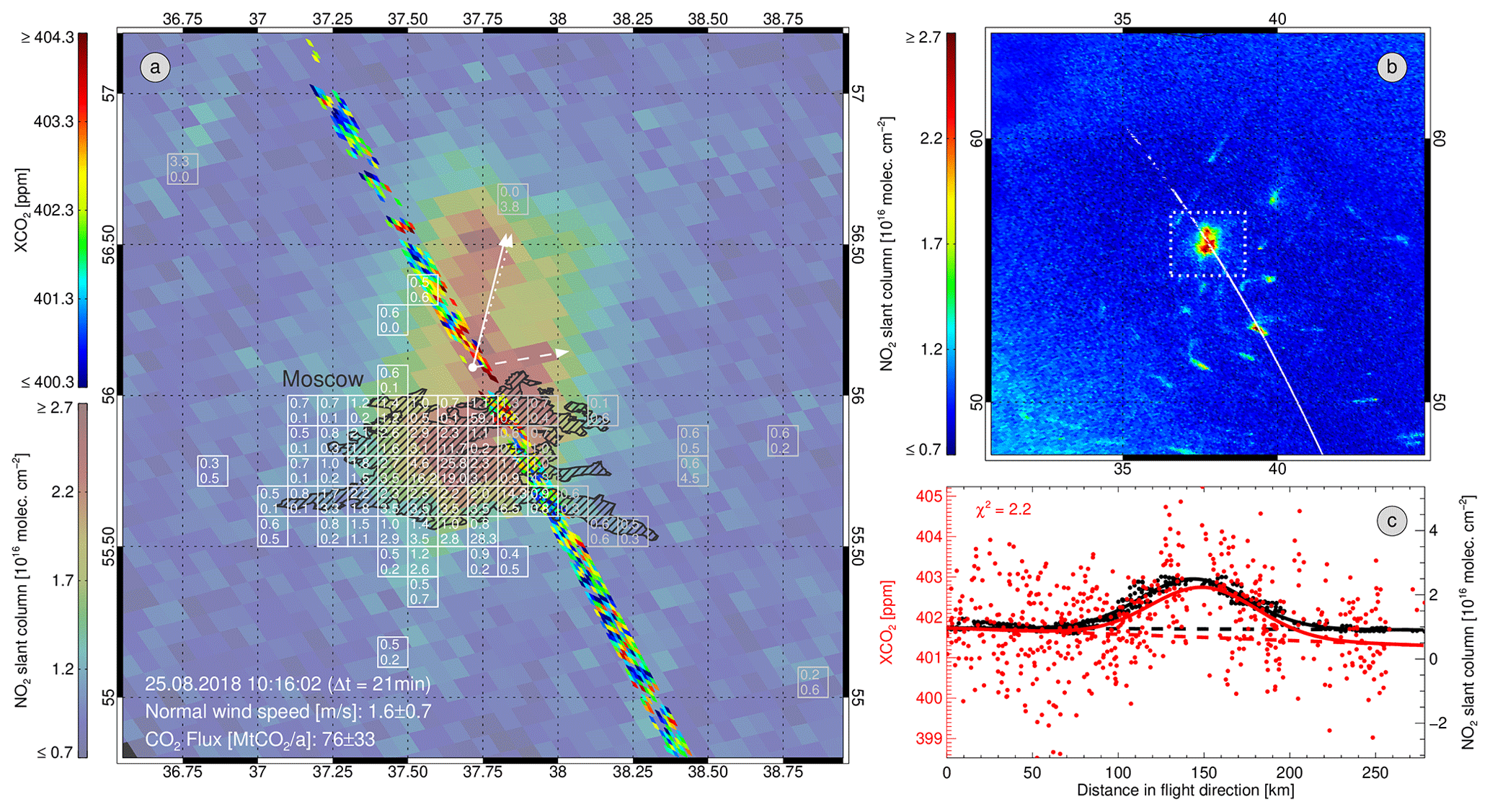
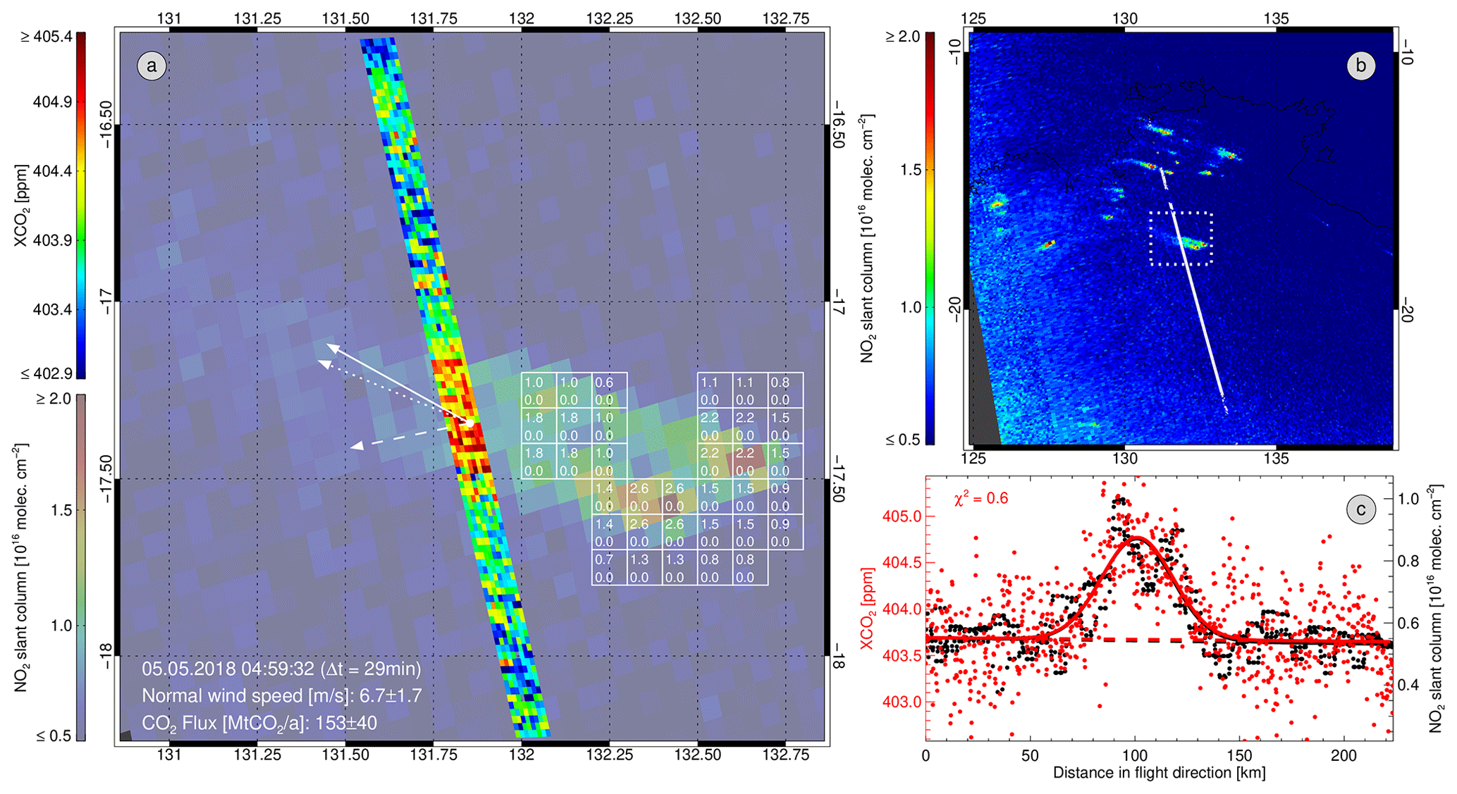
Figure 1Moscow on 25 August 2018. (a) S5P NO2 slant column (background, pale colors) overlaid by OCO-2 XCO2 (foreground, saturated colors). Gray and white 0.1∘ boxes show EDGAR (bottom number in each box) and ODIAC (top number in each box) 2012 annual emissions with either EDGAR or ODIAC being larger than 0.5 MtCO2 a−1. The white arrows show the direction of the 10 m wind as read from ECMWF (dotted), manually corrected to (subjectively) best match the NO2 plume (solid), and normal to the OCO-2 orbit (dashed). Effective wind speed normal to the OCO-2 orbit, estimated cross-sectional CO2 flux, time of OCO-2 overpass, and time difference between OCO-2 and S5P overpass are also listed. The hatched area corresponds to the urban area (World Urban Areas dataset, Geoportal of the University of California, https://apps.gis.ucla.edu/geodata/dataset/world_urban_areas). (b) Larger section of the S5P NO2 slant columns including the OCO-2 orbit and the bounding box of (a). (c) OCO-2 XCO2 values (red) and co-located S5P NO2 slant columns (black) within the plume's cross section in OCO-2 flight direction.
2.2 NO2
The TROPOspheric Monitoring Instrument (TROPOMI) on Sentinel-5 Precursor was launched in October 2017 into a sun-synchronous orbit with an ascending-node Equator crossing time of 13:30 LT (Veefkind et al., 2012). TROPOMI is a nadir-viewing grating imaging spectrometer for the UV–visible spectral region with additional channels in the NIR and SWIR, extending the existing data records of the GOME (Global Ozone Monitoring Experiment), SCIAMACHY, OMI (Ozone Monitoring Instrument), and the GOME-2 missions. It has a swath width of about 2600 km and in comparison to previous instruments a much better spatial resolution of 3.5 km × 7 km at nadir at a similar signal-to-noise ratio per measurement. Here we use radiances in the spectral region 425–465 nm to retrieve NO2 slant columns with a standard Differential Optical Absorption Spectroscopy (DOAS) retrieval developed for previous satellite instruments (Richter et al., 2011), followed by a de-striping step, as described by Boersma et al. (2007). Slant columns are defined as the absorber concentration integrated along the light path, and thus depend on both the atmospheric NO2 profile and the light path of the individual measurement.
The random noise of our S5P slant columns has been estimated from the scatter of observations over a clean Pacific region (10∘ S–10∘ N, 160–230∘ E). In order to account for the viewing-angle dependency of the slant columns, a geometric air mass factor has been computed using only the instrument's viewing zenith angle. The evaluation suggests that the random noise (1σ) of our S5P slant column product is typically 5×10¹⁴ molec. cm−2, while enhancements near sources often exceed 1016 molec. cm−2. For individual soundings, the uncertainty can differ depending on viewing geometry and surface reflectance.
Usually, in order to extract the tropospheric vertical columns, first the stratospheric contribution to the retrieved slant columns needs to be removed and then the light path dependency of the remaining tropospheric slant columns is corrected for by dividing through a scene dependent air mass factor. In this study, another approach is taken as only localized enhancements are evaluated. By subtracting the surrounding background values (Sect. 2.5), both the stratospheric contribution and any tropospheric background are removed from the signal as they are both smooth on the scale of a few tens of kilometers discussed here. What remains is the slant column plume signal of the lower troposphere from which we derive information on the CO2 plume.
2.3 Co-location of OCO-2 and S5P data
OCO-2 and S5P both fly in sun-synchronous orbits with similar Equator crossing times of their ascending nodes and with orbit times of about 100 min. S5P has a swath width of about 2600 km, which provides nearly global coverage each day. For these reasons, each scene observed by OCO-2 is also observed by S5P within a maximum time difference of about 50 min. We project the S5P and OCO-2 data of the same day in a surroundings of a potential target on a high-resolution () grid to compute NO2 averages representative for the footprints of the CO2 soundings (see Fig. 1c for an example).
2.4 Geophysical databases
As input for the computation of the cross-sectional fluxes (Sect. 2.5), we compute the number of dry air particles in the atmospheric column from meteorological profiles which we read at the same time with the wind information from the ECMWF (European Centre for Medium range Weather Forecast) ERA5 (fifth-generation of ECMWF atmospheric reanalyses) data archive at hourly resolution. This data archive also provides an uncertainty estimate of the wind information from an ensemble statistic but at a reduced resolution of about over 3 h.
We compare the inferred cross-sectional CO2 fluxes with the following emission databases. The Emissions Database for Global Atmospheric Research (EDGAR v4.3.2, https://edgar.jrc.ec.europa.eu, last access: 17 July 2019) provides information on anthropogenic CO2 emissions at annual resolution. EDGAR v4.3.2 ends in 2012 and we use the data of that year for our comparisons. The Open-Data Inventory for Anthropogenic Carbon dioxide (ODIAC v2017, http://db.cger.nies.go.jp/dataset/ODIAC (last access: 17 July 2019), Oda et al., 2018) also provides information on annual anthropogenic CO2 emissions but at a finer resolution (1 km × 1 km monthly), and the database ends in 2016. For the reason of comparability, we re-gridded the ODIAC emissions to the EDGAR resolution (0.1∘ × 0.1∘ annually) and use 2012 data as baseline. Additionally, we use ODIAC v2017 data re-gridded to 0.1∘ × 0.1∘ monthly resolution. The Global Fire Emissions Database (GFED v4.1s, https://www.globalfiredata.org, last access: 17 July 2019) provides information on CO2 emissions from wildfires at a resolution of 0.25∘ × 0.25∘ over 3 h, which we re-gridded to 0.1∘ × 0.1∘ resolution for a 6 h average, ending approximately at the time of the overpass.
2.5 Flux estimation
S5P's spatial resolution is considerably coarser than that of OCO-2. Consequently for our case studies, we concentrate on plumes that are significantly larger than the swath width of OCO-2. This means that for the selected scenarios, OCO-2 actually sees only a cross section of a plume (see Fig. 1c for an example).
We model the cross-sectional NO2 columns along the OCO-2 orbit via a linear polynomial, accounting for large-scale variations in the background values, overlaid by a Gaussian function describing the enhancement within the plume. Simultaneously, the cross-sectional CO2 concentrations are modeled in a similar manner. However, the width of the CO2 Gaussian function is constrained to equal the width of the NO2 Gaussian function. This means that the plume shape is determined from the NO2 measurements, but we allow for a shifted position of the maximum in order to account for potential plume displacements resulting from different overpass times. Additionally, it should be noted that the CO2 and NO2 plumes may have small differences, e.g., due to different decay rates of NO2 in different altitudes. These differences, however, are considered minor compared with the precision of the XCO2 soundings. Specifically, the co-located NO2 and XCO2 values along the distance in OCO-2's flight direction x are fitted with the maximum likelihood method by the following vector function:
The free fit parameters a0–8 correspond to the polynomial coefficients of the background values (), the amplitudes (a2, 7), shifts (a3, 8), and the full width at half maximum (FWHM, a4) of the Gaussian functions. We force the FWHM to be constrained entirely by the NO2 measurements by setting the CO2 part of the corresponding Jacobian artificially to zero. However, we expect only little differences with a combined FWHM fit because of the lower relative noise of the NO2 measurements.
Integration over the Gaussian enhancement results in the cross-sectional CO2 flux (mass of CO2 over time) of the plume depending on the FWHM a4, the amplitude of the XCO2 enhancement a7, the effective wind speed ve within the plume normal to the OCO-2 orbit, and the number of dry air particles in the atmospheric column ne:
Here, is the molar mass of CO2 (44.01 g mol−1) and NA is the Avogadro constant (6.02214076 × 10²³ mol−1). We approximate the number of dry air particles ne and the effective wind speed's normal ve from ECMWF ERA5 meteorological profiles at the position of the maximum of the fitted Gaussian XCO2 function. In regions with large variations in surface elevation or wind conditions within the plume's cross section, it might be appropriate to account for variations in the number of dry air particles and/or the wind conditions when integrating over the Gaussian enhancement.
We manually adjust the ECMWF wind direction (not the wind speed) to subjectively fit the plume direction observed in the NO2 fields (e.g., Fig. 1a). The manual adjustment to wind direction but not wind speed is similar to the approaches of, e.g., Krings et al. (2011) or Nassar et al. (2017).
For a hydrostatic atmosphere with a standard surface pressure of 1013 hPa, ne is about 2.16 × 1025 cm−2 and the cross-sectional CO2 flux (Eq. 2) in units of MtCO2 a−1 becomes approximately
given that the FWHM a4, the amplitude of the XCO2 enhancement a7, and the effective wind speed ve are provided in the units km, ppm, and m s−1, respectively. As ne approximately scales with the surface pressure, Eq. (3) may be easily adapted to other meteorological conditions.
As discussed by Brunner et al. (2019), the plume height (and subsequently the wind speed in plume height) depends on many aspects like emission height, stack geometry, flue gas exit velocity and temperature, meteorological conditions, etc. Some of these parameters are not known for many sources and their explicit consideration would go beyond the scope of this study focusing on demonstrating the benefits of simultaneous NO2 and XCO2 measurements rather than on most accurate flux estimates. Varon et al. (2018) proposed approximating the effective wind speed within the plume from the 10 m wind by applying a multiplier in the range of 1.3–1.5. Therefore, we decided to use a multiplier of 1.4 for convenience. This empirical relationship accounts for plume rise and mixing into altitudes with larger wind speeds, for example. For the present, we consider this approximation adequate for this first study, but we recognize that uncertainties (see next section) resulting from this estimate of the effective wind speed's normal may be reduced in the future by improved wind knowledge.
Additionally, it should be noted that the plume cross-sectional flux (Eq. 2) is only a good approximation for the actual source emission under steady-state (temporally invariant) conditions for wind speeds greater than about 2 m s−1 (Varon et al., 2018), when advection dominates over diffusion (Sharan et al., 1996). Changes in wind direction, wind speed, or atmospheric stability in the time span between emission and observation may result in differences between the plume cross-sectional flux and the source flux. Temporal variations in the source emissions of course also result in (temporally delayed) variations in the plume cross-sectional flux, which is always only a snapshot and must not be confused with, e.g., the annual average, even though it is given in the same units. In case of chemically active species (such as NO2), chemical processes along the plume path would also have to be considered in order to compute source emissions from plume cross-sectional fluxes.
2.6 Uncertainty propagation
In order to estimate the uncertainty of the CO2 plume cross-sectional flux (, Eq. 2), we propagate the uncertainties of the FWHM (a4), the amplitude (a7), and the wind speed normal (ve) by assuming uncorrelated errors. The uncertainties of the FWHM and the amplitude result from the maximum likelihood fitting method propagating the uncertainties of the individual XCO2 and NO2 soundings as reported in the data products. The uncertainties of the wind components are read from the ECMWF ERA5 data archive resulting in total wind speed uncertainties ranging from 0.18 to 0.33 m s−1 for the analyzed scenarios. Additionally, we assume that the manual adjustment of the wind direction is accurate by ±10∘. These uncertainties propagate into the uncertainty of the wind speed normal. Varon et al. (2018) estimated that computing the effective wind speed from the 10 m wind introduces an additional uncertainty of 8 %–12 %. However, we analyze scenarios with larger plume structures and probably also larger variations in the injection heights, which we consider by enhancing this error component to 20 % for convenience. Uncertainties in the number of dry air particles are neglected as they are much smaller compared to the wind speed uncertainty, for example. As mentioned earlier, the assumption of constant meteorological conditions might not be valid in regions with large variations in surface elevation or wind conditions within the plume's cross section, which may result in an underestimation of the total cross-sectional flux uncertainty in such cases.
2.7 Plume detection and scenario selection
We use a semiautomatic method to select potentially interesting targets. In a first step, all co-locations of OCO-2 and S5P are computed similarly to those described in Sect. 2.3 but based on a coarser high-resolution grid (0.01∘ × 0.01∘) to improve the computational efficiency. We shift a 30 s (∼200 km) search window in time steps of 0.25 s (∼2 km) over the time series of co-locations. Only those time steps are further considered that have at least 100 co-locations without data gaps exceeding 3 s (∼20 km) within the search window. In the next step, we perform a least-squares fit of the co-located XCO2 and NO2 data with a Gaussian vector function. This fitting function corresponds to Eq. (1) but with independent FWHM for XCO2 and NO2 and centered within the search window (a3 and a8 set to zero), which improves the convergence rate. Only those time steps that fulfill the following criteria are considered further: the fit converges, the NO2 amplitude exceeds 1015 molec. cm−2, the XCO2 and NO2 FWHM (ac and an, respectively) do not exceed the half width of the search window ( s) and do not differ by more than their average (), and the XCO2 and NO2 amplitudes are at least 2 times larger than their uncertainties and larger than the maximum variations in the backgrounds. In the last step, we decided by manual inspection of the XCO2 and NO2 co-locations plus the surrounding NO2 fields and ECMWF wind information if the scenario is a promising candidate for further flux analyses. Potential reasons to reject an automatically preselected scenario are, e.g., too low wind speed, wind direction nearly parallel to OCO-2 orbit, unclear source attribution, or poor fit quality. In total, we manually identified about 20 promising scenarios in the time period January to August 2018 of which we selected and analyzed six examples for this study.
From the time period of January to August 2018, we selected the following scenarios as examples for flux analyses based on co-located XCO2 and NO2 observations.
3.1 Moscow
Figure 1a shows the NO2 enhancement in the city plume of Moscow (approx. 12.4 million inhabitants) as retrieved from S5P overlaid by OCO-2's XCO2 measurements. The NO2 enhancement is clearly also visible in the plume's cross section along OCO-2's ground track (Fig. 1c). Due to the larger relative noise of the XCO2 retrievals, the XCO2 enhancement is less obvious but still visible (Fig. 1c). The Gaussian fit of the enhancements is excellent for NO2 and reasonable (χ2=2.2) for XCO2. There was nearly no adjustment needed (1∘) to bring the ECMWF 10 m wind in good agreement with the NO2 plume (Fig. 1a). The effective wind speed normal to the OCO-2 orbit amounts to 1.6±0.6 m s−1, which is a bit lower than optimal for reasonable flux estimates (Varon et al., 2018). The cross-sectional CO2 flux amounts to 76±33 MtCO2 a−1. This compares to 2012 average upwind emissions (white boxes in Fig. 1a) of 195 MtCO2 a−1 (EDGAR) and 102 MtCO2 a−1 (ODIAC). ODIAC's emission estimate for August 2016 amounts to 88 MtCO2 a−1. The NO2 far field shows no indications of overlaid CO2 plumes from other sources (Fig. 1b). The total flux uncertainty is dominated by the uncertainty of the wind direction followed by the uncertainty of the effective wind speed.
3.2 Lipetsk
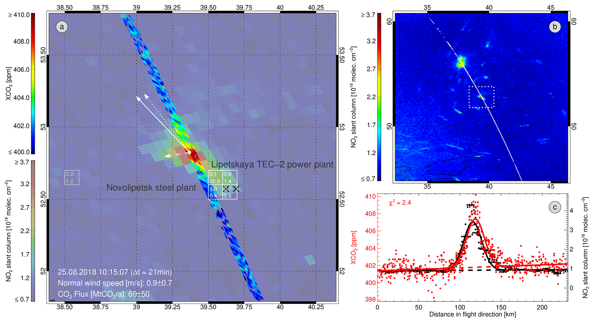
Figure 2a shows the surroundings of Lipetsk (approx. 0.5 million inhabitants) with, among other industries, the Novolipetsk steel plant and the Lipetskaya TEC-2 gas-fired power plant (515 MW) only 1 min (∼400 km) away from Moscow along OCO-2's flight track (see also Fig. 1b). The cross-sectional NO2 and XCO2 enhancements clearly stand out from the noise in the data (Fig. 2c) and the Gaussian function fits the XCO2 data reasonably well (χ2=2.4). We applied a small correction of 5∘ to the ECMWF wind direction. However, as the wind direction is similar to OCO-2's flight direction, the normal effective wind speed is unfavorably low (0.9±0.7 m s−1), which makes the cross-sectional flux estimates (69±50 MtCO2 a−1) less reliable and highly uncertain. The largest uncertainty contribution by far comes from the uncertainty of the wind direction. The 2012 average EDGAR and ODIAC upwind emissions (white marked boxes in Fig. 2a) are 23 and 4 MtCO2 a−1 (same for August 2016), respectively, but the NO2 far field shows no indications of overlaid CO2 plumes from other sources (Fig. 2b).
3.3 Baghdad
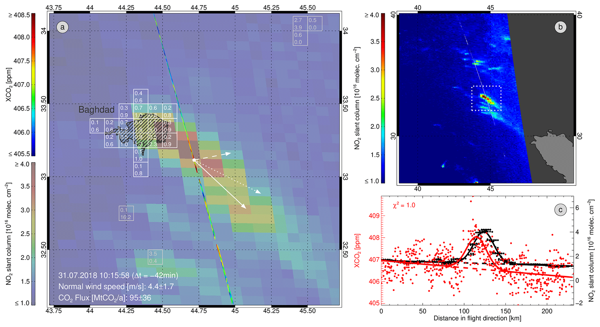
Figure 3a shows the S5P NO2 slant columns overlaid by OCO-2 XCO2 data in a surroundings of Baghdad (approx. 5.4 million inhabitants). Enhanced values are clearly visible in the cross section of the NO2 plume and less obviously also visible in the XCO2 data (Fig. 3c). The XCO2 enhancement is well-fitted (χ2=1.0) by the Gaussian fitting function. The manually adjusted wind direction deviates by 17∘ from the ECMWF wind direction and the normal wind speed amounts to 4.4±1.7 m s−1. From the XCO2 enhancement and the normal wind speed, we compute the cross-sectional CO2 flux to be 95±36 MtCO2 a−1. This compares to an upwind source of 22 or 13 MtCO2 a−1 (12 MtCO2 a−1 for July 2016) of EDGAR or ODIAC, respectively. The flux uncertainty is dominated by the uncertainty of the wind direction and the uncertainty of the effective wind speed. The NO2 far field shows no indications of overlaid CO2 plumes from other sources (Fig. 3b).
3.4 Medupi and Matimba power plants
The Medupi (4764 MW) and Matimba (3990 MW) coal-fired power plants lie close to each other in South Africa, about 300 km north of Johannesburg. Their NO2 plume is shown in Fig. 4a overlaid by OCO2 XCO2 measurements. NO2 measurements in the larger surrounding do not suggest any additional nearby upwind sources (Fig. 4b). The cross-sectional NO2 values show a clear elevation within the plume that is less obvious for XCO2, which has larger relative scatter, especially south of the plume. Nevertheless, the Gaussian function fits the XCO2 values reasonably well (χ2=1.4). The wind direction (corrected by 13∘) is nearly perpendicular to the OCO-2 orbit and the effective normal wind speed is 2.6±0.6 m s−1. The cross-sectional CO2 flux amounts to 31±7 MtCO2 a−1, which is consistent with ODIAC 2012 emissions of 24 MtCO2 a−1 and ODIAC July 2016 emissions of 26 MtCO2 a−1 but EDGAR does not have significant emissions in this area. It should be noted that the Medupi power plant started operation in 2015 with limited capacity and that it still has not reached its nominal capacity. Therefore, it is no surprise that the Medupi power station is not included in either EDGAR or ODIAC 2012 data. The flux uncertainty is dominated by the uncertainty of the effective wind speed.
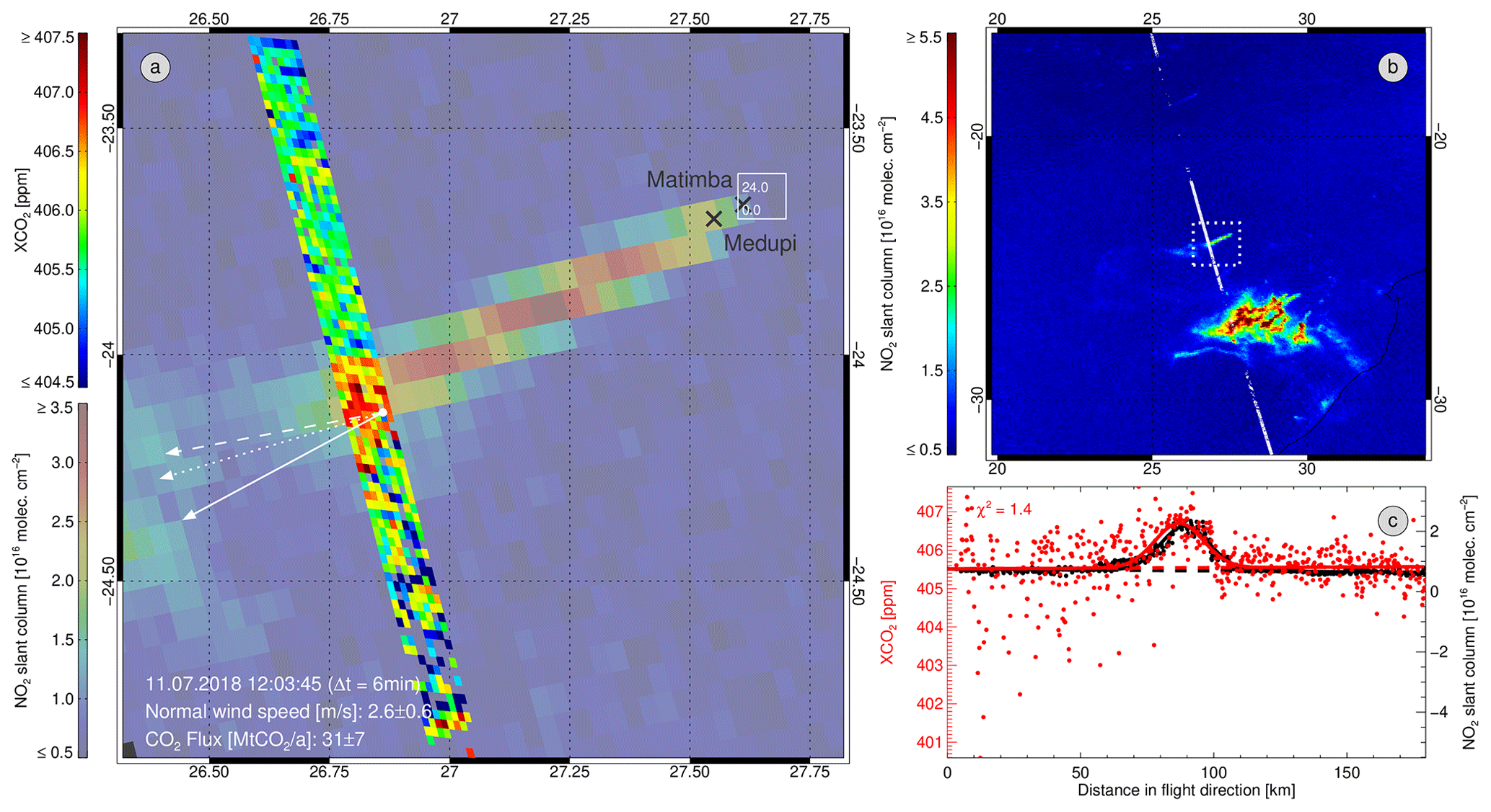
Figure 4As in Fig. 1 but for the Medupi and Matimba power plants in South Africa on 11 July 2018.
3.5 Australian wildfires
Figure 5a shows the NO2 plumes of two Australian wildfires on 5 May 2018 overlaid by an OCO-2 orbit of XCO2 measurements. Enhanced NO2 and XCO2 values are clearly visible within the plume's cross section (Fig. 5b). The NO2 (and also less obviously the XCO2) cross section has two maxima that cannot be accounted for by the Gaussian fitting function. However, this is not reflected in the good XCO2 fit quality (χ2=0.6) but should be taken into account when valuing the results. We applied a small manual correction of 7∘ to the wind direction and the effective wind speed normal to the OCO-2 orbit is 6.7±1.7 m s−1. For the snapshot of the overpass, we computed a cross-sectional CO2 flux of 153±40 MtCO2 a−1. Its uncertainty is driven by the uncertainty of the effective wind speed and wind direction. As the shown plumes originate from wildfires, EDGAR and ODIAC do not include their emissions. However, GFED has average emissions of 52 MtCO2 a−1 within the 6 h period 00:00–06:00 UTC including the time of the overpass (05:00 UTC). The maximum GFED emissions are approximately at the position of the largest NO2 concentrations. Figure 5c shows no indications that additional upwind sources explain the discrepancy between our cross-sectional flux estimate and GFED.
3.6 Nanjing
Figure 6a shows the NO2 slant columns in the surroundings of Nanjing (approx. 5.8 million inhabitants) overlaid by OCO-2 XCO2 measurements. The cross section along the OCO-2 orbit shows strong XCO2 and NO2 plume signals distinctively above the noise level that are well-fitted with the Gaussian fitting function (χ2=0.6). The ECMWF wind direction is not far from being rectangular to the OCO-2 orbit, and we applied a moderate manual correction of 11∘. The effective normal wind speed is 2.2±0.5 m s−1. This results in a cross-sectional flux estimate of 120±27 MtCO2 a−1, which lies in between the upwind emissions of EDGAR (163 MtCO2 a−1) and ODIAC (89 MtCO2 a−1 for 2012, 96 MtCO2 a−1 for March 2016). Figure 6b does not indicate additional major remote upwind sources. The uncertainty of the cross-sectional flux estimate is dominated by the uncertainty of the effective wind speed.

Based on six case studies (Moscow, Russia; Lipetsk, Russia; Baghdad, Iraq; Medupi and Matimba power plants, South Africa; Australian wildfires; and Nanjing, China), we demonstrated the usefulness of simultaneous satellite observations of NO2 and the column-average dry-air mole fraction of CO2 (XCO2). For this purpose, we analyzed co-located regional enhancements of XCO2 observed by OCO-2 and NO2 from S5P and estimated the CO2 plume's cross-sectional fluxes. For atmospheric standard conditions, we approximated as a rule of thumb that a Gaussian enhancement of 1 ppm with a width of 1 km at a wind speed (normal to the cross section) of 1 m s−1 corresponds to a plume cross-sectional flux of roughly 0.53 MtCO2 a−1.
For Moscow, we derived a cross-sectional flux of 76±33 MtCO2 a−1, which agrees (within its uncertainty) with ODIAC 2012 emissions of 102 MtCO2 a−1 (88 MtCO2 a−1 for August 2016) but not with EDGAR emissions of 195 MtCO2 a−1. The cross-sectional flux estimate of Lipetsk with the Novolipetsk steel plant and the Lipetskaya TEC-2 power plant is 69±50 MtCO2 a−1. Within its uncertainty, this estimate agrees with EDGAR emissions of 23 MtCO2 a−1 but not with ODIAC emissions of 4 MtCO2 a−1. However, the uncertainty of the estimate is large due to a wind direction with an acute angle relative to the OCO-2 orbit, which also results in a low effective normal wind speed. This can serve as an example for low wind speeds being favorable for plume detection but not necessarily for flux quantification. In the case of Baghdad, we derived a cross-sectional flux of 95±36 MtCO2 a−1 for the time of the overpass, which is considerably larger than the annual average EDGAR (22 MtCO2 a−1) and ODIAC (13 MtCO2 a−1 for 2012, 12 MtCO2 a−1 for July 2016) emissions of 2012. The wind conditions were relatively good and S5P NO2 measurements do not suggest an overlaying significant upwind source. In this context, it is interesting to note that Georgoulias et al. (2019) found a strongly increasing trend (17.0±0.8 % ∕ a in the period April 1996–September 2017) for the tropospheric NO2 concentrations in Baghdad (and a decreasing trend of % ∕ a for Iraq) hinting at strongly increasing CO2 emissions in Baghdad since 2012. The cross-sectional flux of the plume of the Medupi and Matimba power plants have been estimated to 31±7 MtCO2 a−1, which agrees (within its uncertainty) with ODIAC (24 MtCO2 a−1 for 2012, 26 MtCO2 a−1 for July 2016) but not with EDGAR (no significant emission). Nassar et al. (2017) also estimated the emissions from the Matimba power plant (but not Medupi) using OCO-2 XCO2 v7 data. For a direct overpass in 2014 and a close flyby (∼7 km away) in 2016, they found fluxes, converted to annual values, of 12.1±3.9 MtCO2 a−1 and 12.3±1.2 MtCO2 a−1, respectively. For the Australian wildfires, we estimated a plume cross-sectional flux of 153±40 MtCO2 a−1, which is about 3 times larger than the GFED estimate (52 MtCO2 a−1) for a 6 h average ending approximately at the time of the OCO-2 overpass. Unfavorable wind conditions or a strong overlaying upwind source can be excluded as a reason for the discrepancy. The same is true for the fact that a double-plume structure has been fitted with a Gaussian function. However, it should be noted that GFED's emission estimate for the same time interval but 1 d before the OCO-2 overpass amounts to 252 MtCO2 a−1. For the Nanjing scenario, we derived a cross-sectional flux of 120±27 MtCO2 a−1, which lies in between ODIAC (89 MtCO2 a−1 for 2012, 96 MtCO2 a−1 for March 2016) and EDGAR (164 MtCO2 a−1). However, the scene includes a larger area of overlaying sources, making source attribution difficult.
The total uncertainty of the derived plume cross-sectional fluxes ranges from 7 to 50 MtCO2 a−1 or in relative measures from 23 % to 72 %. The total uncertainty is always dominated by an uncertainty contribution related to meteorology. Specifically, the (manually adjusted) wind direction or the computation of the effective wind speed from the 10 m wind contribute most to the total uncertainty. The noise of the XCO2 retrievals contributes with only 1 to 8 MtCO2 a−1 to the total error and the noise of the NO2 retrievals contributes 3 times less on average.
It is unlikely that the observed XCO2 enhancements are dominated by uncorrected enhancements due to co-emitted aerosols because the OCO-2 retrieval algorithm accounts for light scattering at optically thin aerosol layers and filters scenes with stronger aerosol contamination. Additionally, Bovensmann et al. (2010) estimated for the proposed CarbonSat (Carbon Monitoring Satellite) instrument that neglecting co-emitted aerosols in power plant plumes results in errors between 0.2 and 2.5 MtCO2 a−1, which is small compared with the derived cross-sectional fluxes and their total uncertainties (Table 1). Aerosols can also effect the S5P NO2 slant columns which is, however, less important for our work because we derive only the plume width and direction from the NO2 observations.
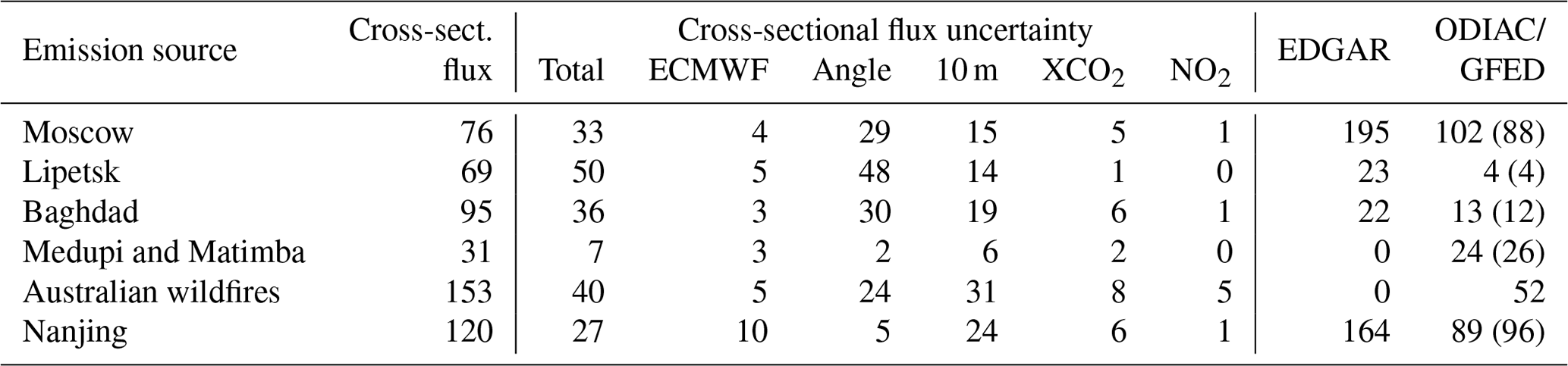
Table 1 Summary of cross-sectional flux results including uncertainty contributions (1σ) and comparison with emission databases EDGAR and ODIAC or GFED in the case of the Australian wildfires. The ODIAC values in brackets represent ODIAC emissions of 2016 and the month of the overpass in the same grid boxes as summed up for 2012. Note that the cross-sectional flux results correspond to the instantaneous time of the overpasses, while EDGAR and ODIAC emissions are annual or monthly averages; GFED emissions correspond to 6 h averages (see Sect. 2.4). The uncertainty estimate is comprised of the total uncertainty and the uncertainties introduced by the ECMWF wind uncertainty, the uncertainty of the wind direction (10∘), use of the 10 m wind (20 %), the XCO2 precision as reported in the data product, and the NO2 precision as reported in the data product. All values are in units of MtCO2 a−1.
It should be noted that differences of the cross-sectional flux estimates and the emission databases are not necessarily coming from inaccuracies of the satellite retrievals or the emission databases. Our estimates are valid only for the time of the overpass, while the emission databases give annual or monthly averages. Velazco et al. (2011) illustrated that power plants can have substantial annual and day-to-day variations. Additionally, the cross-sectional flux is only a good approximation for the source emission under meteorological steady-state conditions with wind speeds greater than about 2 m s−1 (Varon et al., 2018).
For the analyzed scenarios, we observe rather large differences between the EDGAR and ODIAC emission inventories. However, note that only those grid boxes are shown (and summed up) in Figs. 1a–6a for which either EDGAR or ODIAC emissions are larger than 0.5 MtCO2 a−1. This means a smoother distribution of emissions may be misinterpreted as fewer emissions if a significant fraction of the total emission is located in grid boxes not exceeding the 0.5 MtCO2 a−1 threshold. Additionally, it should be noted that ODIAC emissions correspond to fossil fuel combustion and cement production only, while EDGAR also includes emissions from other sectors (e.g., agriculture, land use change, and waste).
NO2 is co-emitted with CO2 when fossil fuels are combusted at high temperatures and has a relatively short lifetime on the order of hours, which makes it a suitable tracer for recently emitted CO2. Despite less strict quality filtering being needed, plume enhancements of NO2 columns near sources can be retrieved from satellites with much lower relative noise than is the case for XCO2. We take advantage of these points by using NO2 measurements to (i) identify the source of the observed XCO2 enhancements, (ii) to exclude interference with potential additional remote upwind sources, (iii) to manually adjust the wind direction, and (iv) to put a constraint on the shape of the observed CO2 plumes.
In principle, it is also possible to fit only the XCO2 values without constraining the plume shape by NO2. In this case, XCO2 is used to derive the amplitude and FWHM of the enhancement. We repeated the flux estimation of all shown scenarios with such a setup and got fluxes of 61±27 MtCO2 a−1, 63±46 MtCO2 a−1, 75±29 MtCO2 a−1, 35±9 MtCO2 a−1, 166±44 MtCO2 a−1, and 119±28 MtCO2 a−1 for the Moscow, Lipetsk, Baghdad, Medupi/Matimba, Australian wildfire, and Nanjing scenarios, respectively. The derived fluxes are consistent within their uncertainty with our main results shown in Table 1, but the uncertainty contribution due to the noise in the XCO2 data increased by 34 % from 4.7 to 6.3 MtCO2 a−1 on average.
Reuter et al. (2014) discussed that post-ENVISAT missions such as OCO-2 would benefit from co-located measurements of co-emitted species from other satellites or (ideally) multispecies measurements from the same instrument. We demonstrated that the analysis of small-scale emissions in OCO-2 XCO2 data indeed profits from simultaneous NO2 observations of S5P as they not only allow us to set the XCO2 observations into context but also to constrain the plume structure. The uncertainties of the cross-sectional flux estimates due to meteorology and their agreement with the actual emissions might be improved in subsequent studies by making use of dedicated simulations with Lagrangian particle dispersion models with either known source positions (and injection heights) or source positions inferred from the NO2 data.
However, we expect the largest room for improvement to be in satellite missions such as the planned European Copernicus anthropogenic CO2 monitoring mission (CO2M), which will provide not only precise measurements with high spatial resolution but also imaging capabilities with a wider swath of simultaneous XCO2 and NO2 observations. Its imaging capabilities will reduce the uncertainty of the inferred emissions due to measurement noise simply because of the increased number of soundings. Additionally, simultaneous XCO2 and NO2 observations from the same platform will allow stricter constraints on the plume shape. More importantly, the meteorology related uncertainties will reduce (Varon et al., 2018) because deviations from steady-state conditions can average out and are, therefore, less critical if the entire plume structure is sampled rather than only a cross section.
The research data used are available at the sources specified in the dataset section.
MR designed the experimental setup, performed the data analysis, did the interpretation, and wrote the paper. MB, OS, SK, HB, and JPB gave support for designing the experimental setup and the interpretation and helped improve the paper. AR gave support for the interpretation and helped improve the paper; he also designed and operated the NO2 satellite retrieval. CWOD gave support for the interpretation and helped improve the paper; he also had a central role in the development and operation of the XCO2 satellite retrieval.
The authors declare that they have no conflict of interest.
This work was funded by the State and the University of Bremen. The OCO-2 XCO2 data were produced by the OCO-2 project at the Jet Propulsion Laboratory, California Institute of Technology, and obtained from the OCO-2 data archive maintained at the NASA Goddard Earth Science Data and Information Services Center. This publication contains modified Copernicus Sentinel data (2018). S5P is an ESA mission implemented on behalf of the European Commission. The TROPOMI payload is a joint development by the ESA and the Netherlands Space Office (NSO). The S5P ground-segment development has been funded by ESA and with national contributions from the Netherlands, Germany, and Belgium. ERA5 meteorological profiles have been obtained from the Copernicus Climate Change Service (C3S) operated by the ECMWF. CO2 emission data have been obtained from the EDGAR, ODIAC, and the GFED databases.
The article processing charges for this open-access publication were covered by the University of Bremen.
This paper was edited by Michel Van Roozendael and reviewed by Ray Nassar and one anonymous referee.
Boersma, K. F., Eskes, H. J., Veefkind, J. P., Brinksma, E. J., van der A, R. J., Sneep, M., van den Oord, G. H. J., Levelt, P. F., Stammes, P., Gleason, J. F., and Bucsela, E. J.: Near-real time retrieval of tropospheric NO2 from OMI, Atmos. Chem. Phys., 7, 2103–2118, https://doi.org/10.5194/acp-7-2103-2007, 2007. a
Bovensmann, H., Burrows, J. P., Buchwitz, M., Frerick, J., Noël, S., Rozanov, V. V., Chance, K. V., and Goede, A.: SCIAMACHY – Mission Objectives and Measurement Modes, J. Atmos. Sci., 56, 127–150, https://doi.org/10.1175/1520-0469(1999)056<0127:SMOAMM>2.0.CO;2, 1999. a
Bovensmann, H., Buchwitz, M., Burrows, J. P., Reuter, M., Krings, T., Gerilowski, K., Schneising, O., Heymann, J., Tretner, A., and Erzinger, J.: A remote sensing technique for global monitoring of power plant CO2 emissions from space and related applications, Atmos. Meas. Tech., 3, 781–811, https://doi.org/10.5194/amt-3-781-2010, 2010. a, b
Brunner, D., Kuhlmann, G., Marshall, J., Clément, V., Fuhrer, O., Broquet, G., Löscher, A., and Meijer, Y.: Accounting for the vertical distribution of emissions in atmospheric CO2 simulations, Atmos. Chem. Phys., 19, 4541–4559, https://doi.org/10.5194/acp-19-4541-2019, 2019. a
Buchwitz, M., Schneising, O., Reuter, M., Heymann, J., Krautwurst, S., Bovensmann, H., Burrows, J. P., Boesch, H., Parker, R. J., Somkuti, P., Detmers, R. G., Hasekamp, O. P., Aben, I., Butz, A., Frankenberg, C., and Turner, A. J.: Satellite-derived methane hotspot emission estimates using a fast data-driven method, Atmos. Chem. Phys., 17, 5751–5774, https://doi.org/10.5194/acp-17-5751-2017, 2017. a
Burrows, J. P., Hölzle, E., Goede, A. P. H., Visser, H., and Fricke, W.: SCIAMACHY – Scanning Imaging Absorption Spectrometer for Atmospheric Chartography, Acta Astronaut., 35, 445–451, 1995. a
Ciais, P., Dolman, A. J., Bombelli, A., Duren, R., Peregon, A., Rayner, P. J., Miller, C., Gobron, N., Kinderman, G., Marland, G., Gruber, N., Chevallier, F., Andres, R. J., Balsamo, G., Bopp, L., Bréon, F.-M., Broquet, G., Dargaville, R., Battin, T. J., Borges, A., Bovensmann, H., Buchwitz, M., Butler, J., Canadell, J. G., Cook, R. B., DeFries, R., Engelen, R., Gurney, K. R., Heinze, C., Heimann, M., Held, A., Henry, M., Law, B., Luyssaert, S., Miller, J., Moriyama, T., Moulin, C., Myneni, R. B., Nussli, C., Obersteiner, M., Ojima, D., Pan, Y., Paris, J.-D., Piao, S. L., Poulter, B., Plummer, S., Quegan, S., Raymond, P., Reichstein, M., Rivier, L., Sabine, C., Schimel, D., Tarasova, O., Valentini, R., Wang, R., van der Werf, G., Wickland, D., Williams, M., and Zehner, C.: Current systematic carbon-cycle observations and the need for implementing a policy-relevant carbon observing system, Biogeosciences, 11, 3547–3602, https://doi.org/10.5194/bg-11-3547-2014, 2014. a
Crisp, D., Atlas, R. M., Bréon, F.-M., Brown, L. R., Burrows, J. P., Ciais, P., Connor, B. J., Doney, S. C., Fung, I. Y., Jacob, D. J., Miller, C. E., O'Brien, D., Pawson, S., Randerson, J. T., Rayner, P., Salawitch, R. S., Sander, S. P., Sen, B., Stephens, G. L., Tans, P. P., Toon, G. C., Wennberg, P. O., Wofsy, S. C., Yung, Y. L., Kuang, Z., Chudasama, B., Sprague, G., Weiss, P., Pollock, R., Kenyon, D., and Schroll, S.: The Orbiting Carbon Observatory (OCO) mission, Adv. Space Res., 34, 700–709, 2004. a, b
Georgoulias, A. K., van der A, R. J., Stammes, P., Boersma, K. F., and Eskes, H. J.: Trends and trend reversal detection in 2 decades of tropospheric NO2 satellite observations, Atmos. Chem. Phys., 19, 6269–6294, https://doi.org/10.5194/acp-19-6269-2019, 2019. a
Heymann, J., Reuter, M., Buchwitz, M., Schneising, O., Bovensmann, H., Burrows, J., Massart, S., Kaiser, J., and Crisp, D.: CO2 emission of Indonesian fires in 2015 estimated from satellite-derived atmospheric CO2 concentrations, Geophys. Res. Lett., 44, 1537–1544, 2017. a
Kiel, M., O'Dell, C. W., Fisher, B., Eldering, A., Nassar, R., MacDonald, C. G., and Wennberg, P. O.: How bias correction goes wrong: measurement of XCO2 affected by erroneous surface pressure estimates, Atmos. Meas. Tech., 12, 2241–2259, https://doi.org/10.5194/amt-12-2241-2019, 2019. a
Krings, T., Gerilowski, K., Buchwitz, M., Reuter, M., Tretner, A., Erzinger, J., Heinze, D., Pflüger, U., Burrows, J. P., and Bovensmann, H.: MAMAP – a new spectrometer system for column-averaged methane and carbon dioxide observations from aircraft: retrieval algorithm and first inversions for point source emission rates, Atmos. Meas. Tech., 4, 1735–1758, https://doi.org/10.5194/amt-4-1735-2011, 2011. a
Kuze, A., Suto, H., Nakajima, M., and Hamazaki, T.: Thermal and near infrared sensor for carbon observation Fourier-transform spectrometer on the Greenhouse Gases Observing Satellite for greenhouse gases monitoring, Appl. Optics, 48, 6716, https://doi.org/10.1364/AO.48.006716, 2009. a
Nassar, R., Hill, T. G., McLinden, C. A., Wunch, D., Jones, D., and Crisp, D.: Quantifying CO2 emissions from individual power plants from space, Geophys. Res. Lett., 44, 10045–10053, https://doi.org/10.1002/2017GL074702, 2017. a, b, c
Oda, T., Maksyutov, S., and Andres, R. J.: The Open-source Data Inventory for Anthropogenic CO2, version 2016 (ODIAC2016): a global monthly fossil fuel CO2 gridded emissions data product for tracer transport simulations and surface flux inversions, Earth Syst. Sci. Data, 10, 87–107, https://doi.org/10.5194/essd-10-87-2018, 2018. a
O'Dell, C. W., Eldering, A., Wennberg, P. O., Crisp, D., Gunson, M. R., Fisher, B., Frankenberg, C., Kiel, M., Lindqvist, H., Mandrake, L., Merrelli, A., Natraj, V., Nelson, R. R., Osterman, G. B., Payne, V. H., Taylor, T. E., Wunch, D., Drouin, B. J., Oyafuso, F., Chang, A., McDuffie, J., Smyth, M., Baker, D. F., Basu, S., Chevallier, F., Crowell, S. M. R., Feng, L., Palmer, P. I., Dubey, M., García, O. E., Griffith, D. W. T., Hase, F., Iraci, L. T., Kivi, R., Morino, I., Notholt, J., Ohyama, H., Petri, C., Roehl, C. M., Sha, M. K., Strong, K., Sussmann, R., Te, Y., Uchino, O., and Velazco, V. A.: Improved retrievals of carbon dioxide from Orbiting Carbon Observatory-2 with the version 8 ACOS algorithm, Atmos. Meas. Tech., 11, 6539–6576, https://doi.org/10.5194/amt-11-6539-2018, 2018. a
Pinty, B., Janssens-Maenhout, G., M., D., Zunker, H., Brunhes, T., Ciais, P., Denier van der Gon, D. Dee, H., Dolman, H., M., D., Engelen, R., Heimann, M., Holmlund, K., Husband, R., Kentarchos, A., Meijer, Y., Palmer, P., and Scholze, M.: An Operational Anthropogenic CO2 Emissions Monitoring & Verification Support capacity – Baseline Requirements, Model Components and Functional Architecture, European Commission Joint Research Centre, EUR 28736 EN, available at: https://www.copernicus.eu/sites/default/files/2018-10/Report_Copernicus_CO2_Monitoring_TaskForce_Nov2017_0.pdf (last access: 17 July 2019), 2017. a
Reuter, M., Buchwitz, M., Hilboll, A., Richter, A., Schneising, O., Hilker, M., Heymann, J., Bovensmann, H., and Burrows, J.: Decreasing emissions of NOx relative to CO2 in East Asia inferred from satellite observations, Nat. Geosci., 7, 792, 2014. a, b, c
Reuter, M., Buchwitz, M., Schneising, O., Noël, S., Bovensmann, H., and Burrows, J. P.: A fast atmospheric trace gas retrieval for hyperspectral instruments approximating multiple scattering – Part 2: application to XCO2 retrievals from OCO-2, Remote Sens., 9, 1102, https://doi.org/10.3390/rs9111102, 2017. a, b
Richter, A., Burrows, J. P., Nüß, H., Granier, C., and Niemeier, U.: Increase in tropospheric nitrogen dioxide over China observed from space, Nature, 437, 129–132, https://doi.org/10.1038/nature04092, 2005. a
Richter, A., Begoin, M., Hilboll, A., and Burrows, J. P.: An improved NO2 retrieval for the GOME-2 satellite instrument, Atmos. Meas. Tech., 4, 1147–1159, https://doi.org/10.5194/amt-4-1147-2011, 2011. a
Rockström, J., Gaffney, O., Rogelj, J., Meinshausen, M., Nakicenovic, N., and Schellnhuber, H. J.: A roadmap for rapid decarbonization, Science, 355, 1269–1271, 2017. a
Schneising, O., Heymann, J., Buchwitz, M., Reuter, M., Bovensmann, H., and Burrows, J. P.: Anthropogenic carbon dioxide source areas observed from space: assessment of regional enhancements and trends, Atmos. Chem. Phys., 13, 2445–2454, https://doi.org/10.5194/acp-13-2445-2013, 2013. a
Sharan, M., Yadav, A. K., Singh, M., Agarwal, P., and Nigam, S.: A mathematical model for the dispersion of air pollutants in low wind conditions, Atmos. Environ., 30, 1209–1220, 1996. a
Varon, D. J., Jacob, D. J., McKeever, J., Jervis, D., Durak, B. O. A., Xia, Y., and Huang, Y.: Quantifying methane point sources from fine-scale satellite observations of atmospheric methane plumes, Atmos. Meas. Tech., 11, 5673–5686, https://doi.org/10.5194/amt-11-5673-2018, 2018. a, b, c, d, e, f
Veefkind, J. P., Aben, I., McMullan, K., Förster, H., de Vries, J., Otter, G., Claas, J., Eskes, H. J., de Haan, J. F., Kleipool, Q., van Weele, M., Hasekamp, O., Hoogeveen, R., Landgraf, J., Snel, R., Tol, P., Ingmann, P., Voors, R., Kruizinga, B., Vink, R., Visser, H., and Levelt, P. F.: TROPOMI on the ESA Sentinel-5 Precursor: A GMES mission for global observations of the atmospheric composition for climate, air quality and ozone layer applications, Remote Sens. Environ., 120, 70–83, 2012. a, b
Velazco, V. A., Buchwitz, M., Bovensmann, H., Reuter, M., Schneising, O., Heymann, J., Krings, T., Gerilowski, K., and Burrows, J. P.: Towards space based verification of CO2 emissions from strong localized sources: fossil fuel power plant emissions as seen by a CarbonSat constellation, Atmos. Meas. Tech., 4, 2809–2822, https://doi.org/10.5194/amt-4-2809-2011, 2011. a