the Creative Commons Attribution 4.0 License.
the Creative Commons Attribution 4.0 License.
 | 18 Jul 2019
Urban population exposure to NOx emissions from local shipping in three Baltic Sea harbour cities – a generic approach
Martin Otto Paul Ramacher
Matthias Karl
Johannes Bieser
Jukka-Pekka Jalkanen
Lasse Johansson
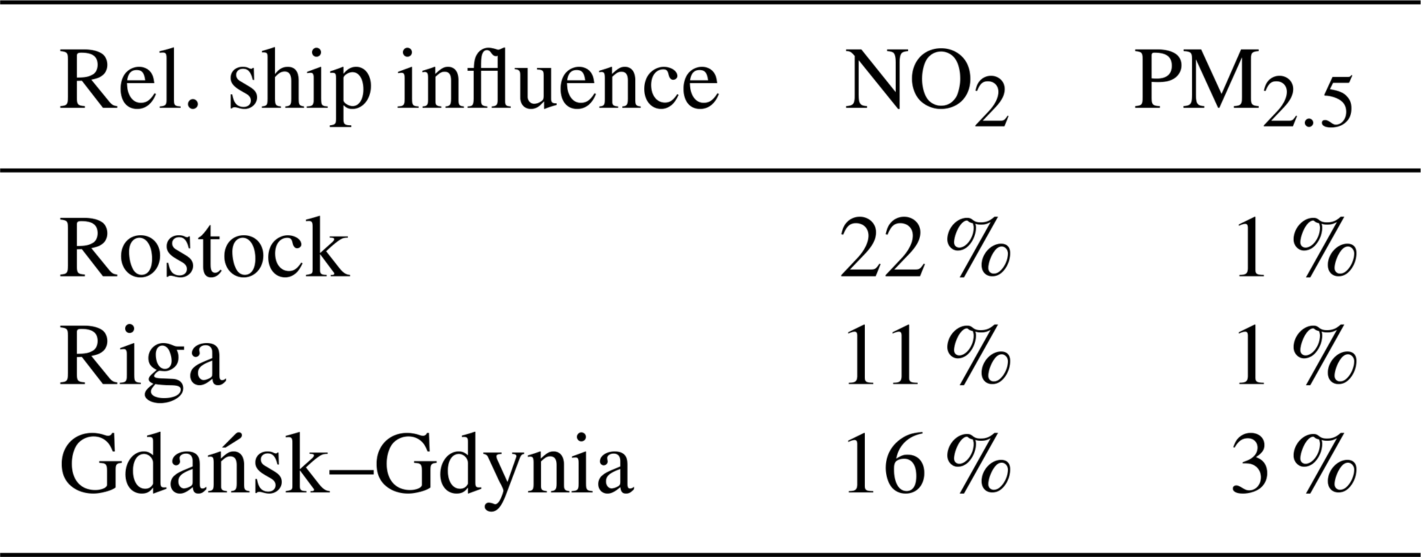
Ship emissions in ports can have a significant impact on local air quality (AQ), population exposure and therefore human health in harbour cities. We determined the impact of shipping emissions in harbours on local AQ and population exposure in the Baltic Sea harbour cities Rostock (Germany), Riga (Latvia) and the urban agglomeration of Gdańsk–Gdynia (Poland) for 2012. An urban AQ study was performed using a global-to-local chemistry transport model chain with the EPISODE-CityChem model for the urban scale. We simulated NO2, O3 and PM concentrations in 2012 with the aim of determining the impact of local shipping activities on population exposure in Baltic Sea harbour cities. Based on simulated concentrations, dynamic population exposure to outdoor NO2 concentrations for all urban domains was calculated. We developed and used a novel generic approach to model dynamic population activity in different microenvironments based on publicly available data. The results of the new approach are hourly microenvironment-specific population grids with a spatial resolution of 100 m × 100 m. We multiplied these grids with surface pollutant concentration fields of the same resolution to calculate total population exposure. We found that the local shipping impact on NO2 concentrations is significant, contributing 22 %, 11 % and 16 % to the total annually averaged grid mean concentration for Rostock, Riga and Gdańsk–Gdynia, respectively. For PM2.5, the contribution of shipping is substantially lower, at 1 %–3 %. When it comes to microenvironment-specific exposure to annual NO2, the highest exposure to NO2 from all emission sources was found in the home environment (54 %–59 %). Emissions from shipping have a high impact on NO2 exposure in the port area (50 %–80 %), while the influence in home, work and other environments is lower on average (3 %–14 %) but still has high impacts close to the port areas and downwind of them. Besides this, the newly developed generic approach allows for dynamic population-weighted outdoor exposure calculations in European cities without the necessity of individually measured data or large-scale surveys on population data.
- Article
(5322 KB) -
Supplement
(373 KB) - BibTeX
- EndNote


According to the International Maritime Organization (IMO), more than 90 % of world trade is carried by sea, since maritime transport is the most cost-effective way to move mass goods and raw materials (International Maritime Organization, 2015). However, maritime transport is an important source of air pollutants on the global (Wang et al., 2008) and European level (Eyring et al., 2010) and can contribute significantly to local air quality (AQ) problems in European harbour cities of all sizes (Viana et al., 2009). Globally, ships are known to emit 5–7×10⁹ kg yr−1 of nitrogen oxides (NOx), 4.7–6.5×10⁹ kg yr−1 of sulfur dioxide (SO2) and 1.2–1.6×10⁹ kg yr−1 of particulate matter (PM) into the atmosphere (Smith et al., 2014; Corbett and Koehler, 2003; Eyring et al., 2005); 70 % of these emissions occur near coastlines and therefore contribute to air pollution in both coastal areas and harbour cities (Andersson et al., 2009; Corbett et al., 1999; Endresen, 2003). Ships emit NOx mainly in the form of NO, which is quickly converted to NO2; thus atmospheric NOx from shipping is mainly in the form of NO2 (Eyring et al., 2010). The contribution of international shipping to the air quality over European seas reached up to 80 % for NOx and SO2 concentrations, up to 25 % for particles with a diameter of 2.5 µm and less (PM2.5), and up to 15 % for ozone (O3) in hotspot areas along coastlines in 2005 (EEA, 2013). In the North Sea region, the relative contribution of international shipping to NO2 concentration levels ashore close to the sea can reach up to 25 % in summer and 15 % in winter (Aulinger et al., 2016), while Karl et al. (2019c) showed average shipping contributions of 40 % over the Baltic Sea and 22 %–28 % for the entire Baltic Sea region. In the entire Baltic Sea region the average contribution of ships to PM2.5 levels is in the range of 4.3 %–6.5 %, (Karl et al., 2019a).
However, little is known about the impact of ship emissions in harbour cities of the North Sea and Baltic Sea region. Even if emissions of in-port ships account for only a few percent of the global emissions related to shipping (Dalsøren et al., 2009), they can have an important impact on local AQ in harbour cities due to additional emissions from manoeuvring, mooring and diesel-powered activities at berth, such as lighting, cooling, heating and sanitation (Meyer et al., 2008). Viana et al. (2014) performed a literature review with the aim of characterising and quantifying the contribution of the maritime transport sector to air quality degradation along European coastal areas. The reviewed studies agreed on the relevance of ship emissions in coastal areas for PM, NOx and SO2 and identified a large spatial variability, with maximal contributions in the Mediterranean Basin and the North Sea. On average, shipping emissions in the coastal North Sea region contribute 7 %–24 % to NO2 annual mean and 3 %–5 % to PM2.5 annual mean concentrations in the North Sea, while in the Mediterranean PM2.5 from shipping contributes 4 %–20 % (Viana et al., 2014).
Only few studies investigated the impact of in-port ship emissions on the AQ in harbour cities of the Baltic Sea. Saxe and Larsen (2004) showed the impact of local shipping activities in Copenhagen, Denmark, which connects the ship traffic between the North Sea and Baltic Sea. NOx from shipping was exceeded 200 µg m−3 of NOx and caused values of 50–200 µg m−3 over several square kilometres of central Copenhagen, while PM and SO2 contributed with insignificant mass concentrations of PM to populated areas near the harbour (Saxe and Larsen, 2004). Pirjola et al. (2014) measured particulate and gaseous emissions from ship diesel engines with different after-treatment systems using a mobile laboratory inside the harbour areas in Helsinki and along the narrow shipping channel near Turku, Finland, and concluded the need for additional regulation of shipping particulate emissions beyond controlling the fuel sulfur content. Also in Helsinki, Soares et al. (2014) investigated the impact of emissions from ship traffic in the harbours of Helsinki and in the surrounding area on concentrations and exposure, identifying a contribution of about 3 % to PM2.5 concentrations by shipping activities.
A more recent study by Ledoux et al. (2018) in the North Sea port of Calais showed the direct influence of in-port shipping on SO2, NO2 and PM10 average concentrations, at 51 %, 15 % and 2 %, respectively, and with substantial concentration peaks synchronised with departures and arrivals of ferries. In the harbour city Hamburg, Ramacher et al. (2018) identified maximum relative contributions from shipping to total NO2 and PM2.5 concentrations, at 23 % and 3 % in January and 45 % and 16 % in July 2012 and with the highest concentrations located in the port area of Hamburg. A study in preparation (Tang et al., 2019) modelled local NO2 shipping contributions to air pollution in the urban area of Gothenburg of about 14 % and a regional NO2 contribution of up to 41 % on average to the annual mean, indicating the same importance in controlling local shipping emissions as, for example, road traffic emissions, while SO2 and PM2.5 contributions are negligible.
Exposure to air pollution can lead to asthma, respiratory and cardiovascular diseases, lung cancer, and premature deaths according to the World Health Organization (WHO, 2006). Corbett et al. (2007) showed that shipping-related PM emissions are responsible for approximately 60 000 cardiopulmonary and lung cancer deaths annually, with most deaths occurring in coastal regions of Europe, eastern Asia and southern Asia. An update of this study shows that despite implemented regulations, low-sulfur marine fuels will account for 250 000 deaths annually in 2020 due to an increase in transport by sea (Sofiev et al., 2018b). Approximately 230 million people are directly exposed to these shipping emissions in the top 100 world ports (Merk, 2014). The large majority (95 %) of Europeans living in urban environments are exposed to levels of air pollution considered dangerous to human health. The average contribution of shipping emissions to the population exposure from primary PM2.5, NOx and SOx is 8 %, 16.5 % and 11 %, respectively, across Europe (Andersson et al., 2009). While exposure to PM2.5 was estimated to be a leading cause of the WHO environmental burden of disease in six selected European countries (Hänninen et al., 2014), the relationship between NO2 and health is scientifically not as well founded as for PM2.5 (WHO, 2006; Heroux et al., 2013). However, NO2 is usually regarded as an indicator of other pollutants, and long-term residential exposure to NOx is moving into focus due to rising evidence for severe health effects on the respiratory system (WHO, 2016; Wing et al., 2018; Hamra et al., 2015) and as risk factor for myocardial infarction (Rasche et al., 2018). In terms of exposure to shipping emissions, NO2 was found to be consistently associated with total non-accidental mortality and specific cardiovascular mortality in the Baltic Sea harbour city Gothenburg (Stockfelt et al., 2015). Thus, exposure to air pollution caused by shipping activities in harbour cities needs to be reduced and emissions regulated.
Regulations for the prevention of air pollution from ships was introduced in the Marine Pollution Convention (MARPOL) Annex VI by the IMO and entered into force in 2005. Many countries have ratified this protocol, particularly for limiting NOx and SO2 emissions from ships. The coastal areas of the North Sea and the Baltic Sea have been classified as sulfur emission control areas (SECAs), where the sulfur content in marine fuels has been limited to 0.1 % from 2015 on. Moreover, the European Union introduced a requirement limiting the sulfur content in fuels used by ships at berth to 0.1 % in 2010. The European Environment Agency (EEA) therefore estimated the decrease in SO2 ship emissions to be 54 % between 2000 and 2010, and a further decrease is expected from 2020 onwards due to changes in technology and global regulations (EEA, 2013). It is also expected that this will lead to a decrease in emissions of PM2.5. Nevertheless, NOx emissions from international maritime transport in European waters are projected to increase and could be equal to land-based sources by 2020. In order to reduce NOx emissions from shipping, an NOx Emission Control Area (NECA) will be implemented in the North Sea and Baltic Sea on 1 January 2021. The goal is to decrease nitrogen oxide emissions from maritime transport by 80 % compared to present levels in the long run. Besides this, an additional reduction in PM2.5 is expected in the future due to less NOx-induced secondary organic aerosol (SOA) formation, which would lower the ship-related PM2.5 by 72 % in 2040, compared to the present, while it would be reduced by only 48 % without implementation of the NECA (Karl et al., 2019c). Despite these regulations to reduce SOx (SECA) and NOx (NECA) emissions in Europe, ship traffic is still the least regulated sector in Europe compared to other types of anthropogenic emission sources such as road traffic, industrial sources, power generation or residential heating. Hence, shipping emissions are increasing in terms of the relative weight of shipping emissions to the total anthropogenic emissions on the regional and local scale in Europe (EEA, 2013). Taking into account the projected increase in maritime transport due to growth of the global-scale trade (Lloyds Register Marine, 2014; EC, 2012) as well as the simultaneous increase in population growth and urbanisation in coastal areas (Neumann et al., 2015), it is necessary to come up with pollution prevention efforts for ports in harbour cities.
The objective of this study is to identify the impact of emissions due to local shipping activities on air quality and population exposure to concentrations of NOx in three major Baltic Sea harbour cities: Rostock (Germany), Riga (Latvia) and the urban agglomeration of Gdańsk–Gdynia (Poland). To identify the impact of local shipping activities on AQ, an urban-scale chemistry transport modelling (CTM) system, was set up for the selected Baltic Sea harbour cities. Besides city-specific emission inventories for land-based emission sources, spatially and temporally high-resolution shipping-emission inventories have been modelled and applied. All study areas are located in the SECA, and the study was performed for 2012 conditions, when the sulfur content in marine fuels was limited to 1 % in the region and 0.1 % for ships at berth. Therefore, and because of the decreasing importance, we excluded SO2 from the study focus. We analysed concentrations of NO2, O3 and PM2.5 for 2012 conditions and evaluated these with local measurement network data of each harbour city. The impact of local shipping activities on urban air quality was determined with the perturbation method (zero-out scenario runs). We focus on the impact of local in-port shipping on the air quality in harbour cities while considering that the influence of ocean-going shipping on the Baltic Sea is beyond the scope of this study. Based on the simulated concentration fields, dynamic population-weighted outdoor exposure to NO2 and PM2.5 for all urban domains was calculated in different microenvironments using a newly developed generic exposure modelling approach based on publicly available data. This study mainly focusses on NO2 exposure, taking into account the high contributions of local shipping activities to NO2 in other harbour cities, the growing importance of NO2 as an indicator for health effects and the usage of NO2 as an indicator for health effects due to other pollutants.
To our knowledge, this study is the first one investigating the impact of emissions from local shipping activities on air pollutant concentrations and population exposure in Baltic Sea harbour cities since the 2010 commencement of the 0.1 % sulfur fuel requirement in harbours (European Parliament Directive 2005/33/EC), using a CTM system with high spatial and temporal resolution.
Section 2 of this paper describes the model and data set-up, introducing the urban-scale CTM EPISODE-CityChem in Sect. 2.1 and describing the set-up of each urban domain in Sect. 2.2 and 2.3. This is followed by the description of local emission inventories and their application in the CTM system (Sect. 2.4 and 2.5). Finally, a new generic approach to achieve outdoor exposure for different microenvironments will be introduced in Sect. 2.7. In Sect. 3, the simulated concentrations will be evaluated (Sect. 3.1), and total as well as ship-related concentration distributions of NO2 and PM2.5 will be presented for the city domains (Sect. 3.2). This is followed by the analysis and illustration of exposure results due to total and ship-related concentrations (Sect. 3.3). Section 4 discusses the exposure results with respect to the novel approach for generic dynamic population activity and is followed by conclusions in Sect. 5.
A CTM system with the EPISODE-CityChem model (Karl et al., 2019b; Karl and Ramacher, 2018) to simulate present day urban concentrations of NO2 and PM2.5 as well as the contribution of shipping activities to urban air quality was set-up for the Baltic Sea urban areas of Rostock, Riga and Gdańsk–Gdynia. City-specific meteorological fields, regional boundary conditions, and land-based emission and shipping-emission inventories have been gathered and modelled. The contribution of present shipping emissions to the modelled concentration of air pollutants was determined from the difference between “base” runs, which include all emissions, and “no-ship” runs, which exclude emissions from ship traffic (zero-out method). The concentration results are then evaluated and used to model dynamic population-level exposure in different microenvironments for each city (Fig. 1).
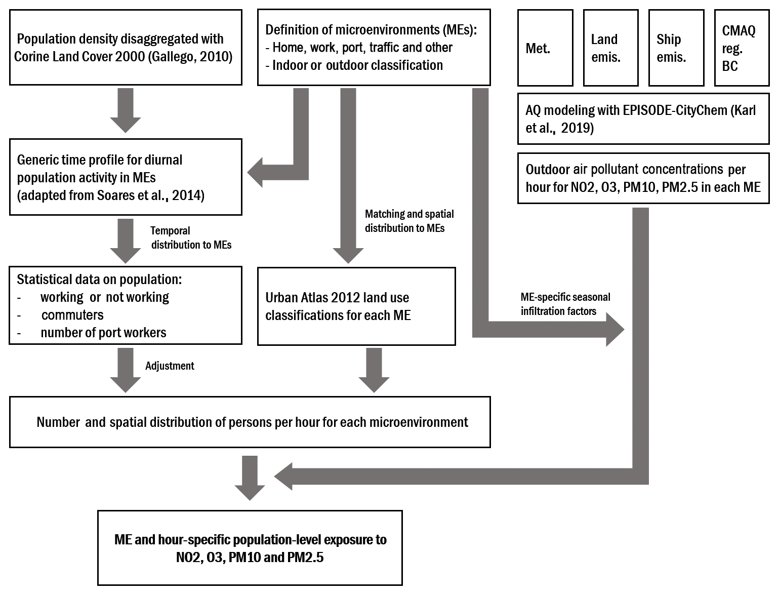
Figure 1Study design to calculate microenvironment-specific population exposure to outdoor air pollution based on CTM concentration simulations and taking into account seasonally changing infiltration factors for indoor environments.
2.1 EPISODE-CityChem
For all harbour cities, the urban-scale CTM EPISODE-CityChem (Karl et al., 2019b) was applied. The city-scale chemistry (CityChem) model is an extension of the urban dispersion model EPISODE of the Norwegian Institute for Air Research (NILU; Slørdal et al., 2003, 2008). A more up-to-date description of EPISODE is in preparation (Hamer et al., 2019). EPISODE systematically combines a 3-D Eulerian grid model with a sub-grid Gaussian dispersion model, allowing for the computation of pollutant concentrations near road traffic line sources and industrial point sources with high spatial resolution. EPISODE-CityChem is capable of modelling the photochemical transformation of multiple pollutants along with atmospheric diffusion to produce pollutant concentration fields for an entire city on a horizontal resolution of 100 m or even finer. The purpose of EPISODE-CityChem is to fill the gap between regional-scale air quality simulations with Eulerian CTM systems (with typical resolutions between 100 and 1000 m) on one hand and micro-scale simulations of limited areas of the urban environment using large eddy simulation (LES) techniques (Nieuwstadt and Meeder, 1997) on the other hand. In order to resolve chemical transformation of reactive pollutants in the proximity of emission source objects (point source and lines sources), the atmospheric chemistry is considered in detail within the Eulerian grid and is considered in a simplified manner for the sub-grid dispersion. The applied chemical scheme in this study is the EmChem03-mod, which is an update of the EMEP45 chemical mechanism (Simpson et al., 2003; Walker et al., 2003) and consists of 45 gas-phase species, 51 thermal reactions and 16 photolysis reactions. Levels of PM2.5 and PM10 in the model are controlled by primary emissions of particulate matter and their atmospheric dispersion, while secondary aerosol formation is not considered in the model (Karl et al., 2019b).
The model reads meteorological fields, either generated by the prognostic meteorology component of the Australian air quality model TAPM (The Air Pollution Model; Hurley, 2008; Hurley et al., 2005) or other diagnostic wind fields, for calculating the dispersion parameters, vertical profile functions in the surface layer and the eddy diffusivities in EPISODE-CityChem. Moreover, EPISODE-CityChem has the option of using the time-varying 3-D concentration field at the lateral and vertical boundaries from the Community Multiscale Air Quality Modelling System (CMAQ; Byun and Schere, 2006) as initial and boundary concentrations for selected chemical species.
Emissions in EPISODE-CityChem can be treated as area sources (2-D area of the size of a grid cell), line sources (line between two (x,y) coordinates) and point sources (industrial and power plant stacks). Moreover, a simplified street canyon model (SSCM) based on the OSPM model (Berkowicz et al., 1997) can be used in EPISODE-CityChem, potentially allowing for a better treatment of NOx at traffic stations. The meteorological preprocessor (WMPP) of the Weak Wind Open Road Model (WORM; Walker, 2011) is used in the point source sub-grid model to calculate the wind speed at plume height for the dispersion of plume segments released from industrial and power plant stacks.
Emission input containing sector-specific (following SNAP nomenclature) and geo-referenced yearly emission totals are preprocessed with the model's interface for emission preprocessing, the Urban Emission Conversion Tool (UECT; Hamer et al., 2019), which produces hourly varying emission input for point sources, line sources and area source categories using sector-specific temporal profiles and vertical profiles.
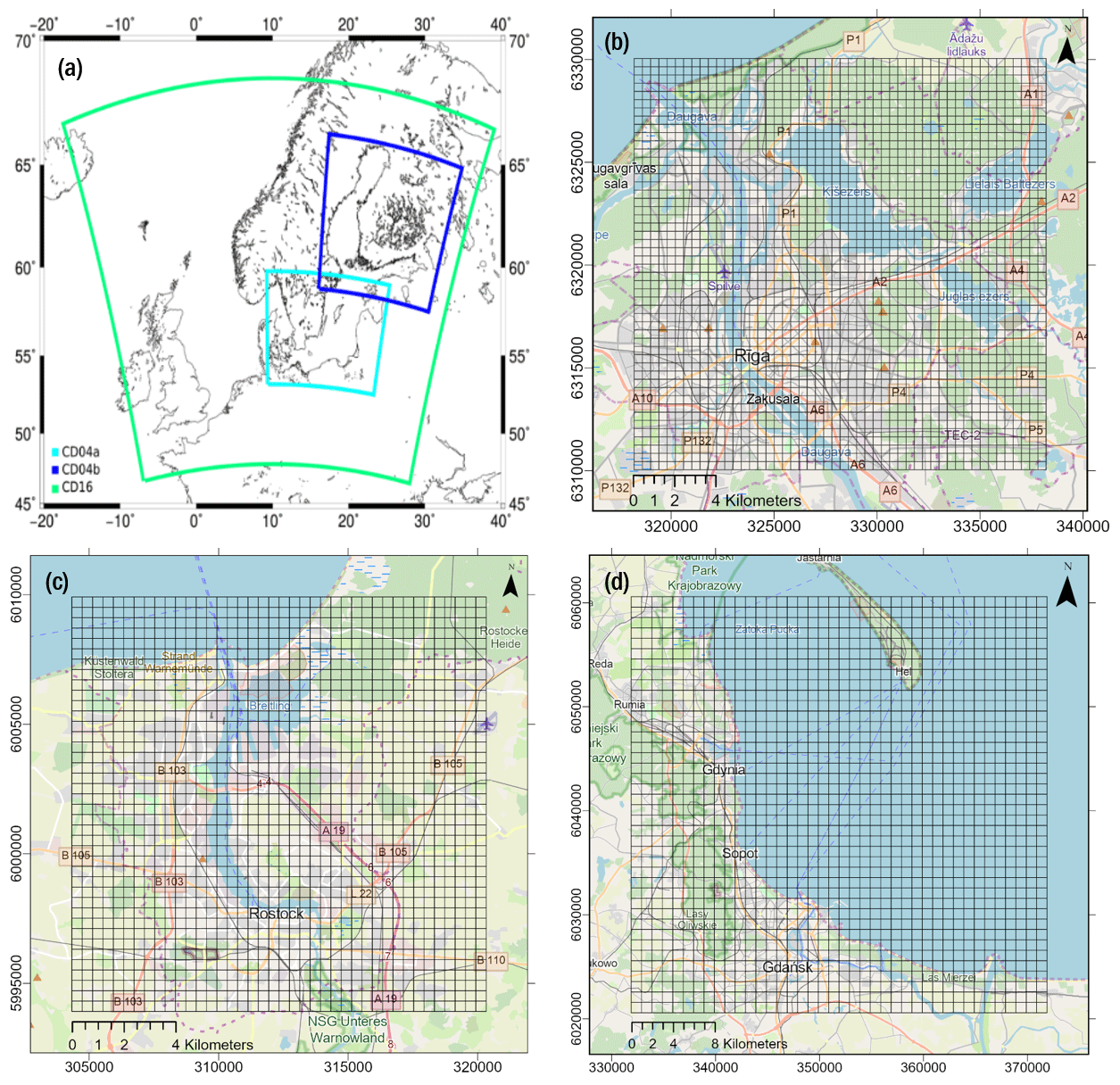
Figure 2(a) Regional CTM simulation domains, which have been used to drive the local-scale EPISODE-CityChem simulation for the urban domains in (b) Riga and (c) Rostock, with 400 m resolution for 20 km × 20 km and 16 km × 16 km extent, and (d) Gdańsk–Gdynia, with 1000 m resolution and 40 km × 40 km extent. Maps are created using © 2018 ESRI Inc. ArcGIS Pro 2.3.2 with a topographic base map by © OpenStreetMap contributors 2019. Distributed under a Creative Commons BY-SA License.
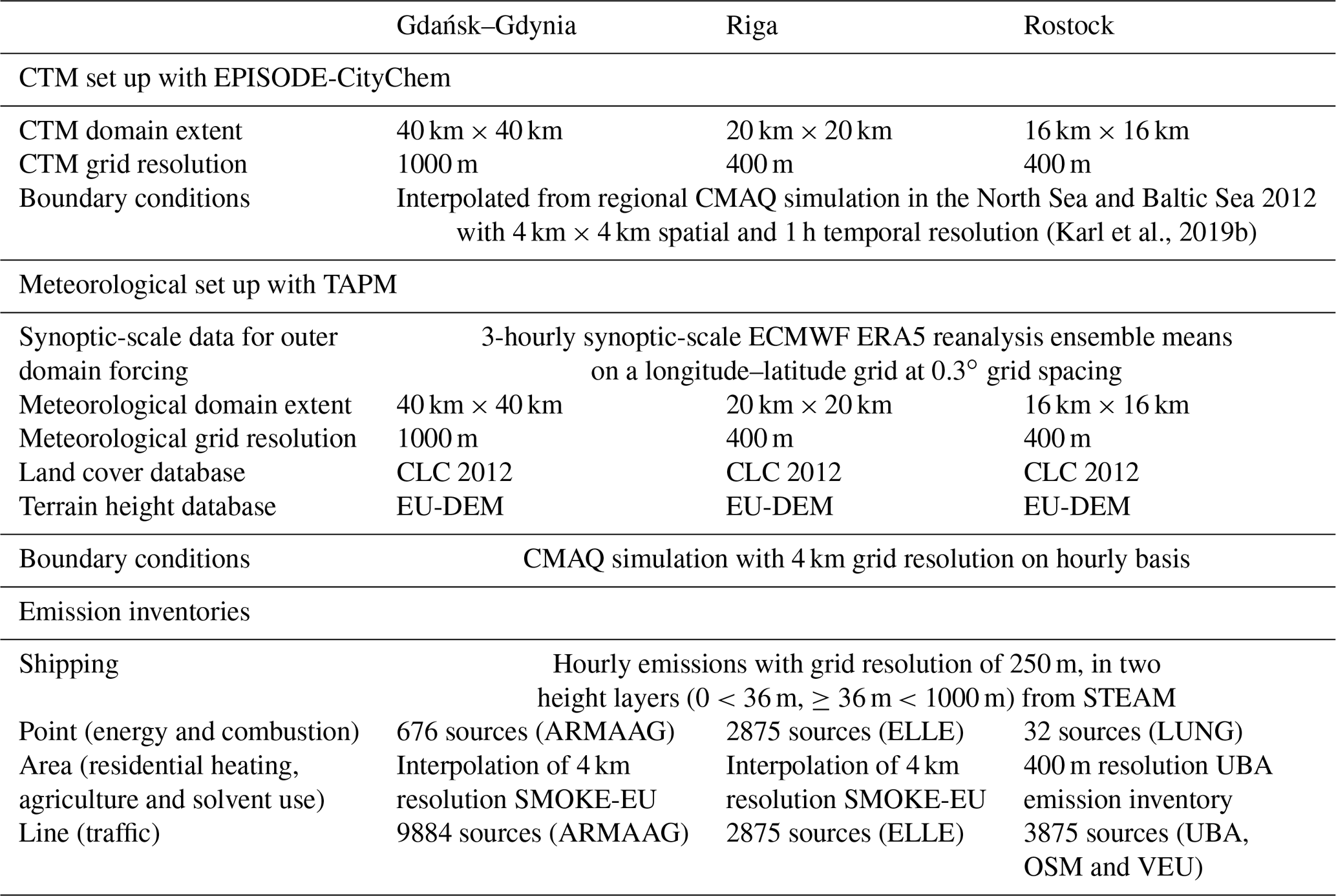
Table 1Overview of EPISODE-CityChem set-up, the TAPM meteorological set-up and emission data for each urban domain.
In this study, we defined three urban domains for CTM simulations with EPISODE-CityChem (Fig. 2). EPISODE-CityChem uses a 2-D Cartesian coordinate system, and therefore we used the Universal Transverse Mercator (UTM) conformal projection to set the geographic dimensions for all research domains. While the model domains for Rostock and Riga were set up for a 16 km × 16 km and a 20 km × 20 km area with 400 m resolution, the model domain for the Gdańsk–Gdynia urban agglomeration was set up for a 40 km × 40 km area with 1 km grid resolution (Table 1). The SSCM for traffic line sources was activated for all simulations, and EPISODE-CityChem provided concentration output and other diagnostic output in netCDF files.
2.2 Meteorology set-up
In this study, the meteorological data for all research domains were provided from the meteorological component of the coupled meteorological and chemistry transport model TAPM. TAPM predicts three-dimensional meteorology based on an incompressible, non-hydrostatic and primitive equation model with a terrain-following vertical coordinate for three-dimensional simulations. The model solves the momentum equations for horizontal wind components; the incompressible continuity equation for vertical velocity; and scalar equations for potential virtual temperature and specific humidity, cloud water and ice, rainwater, and snow (Hurley, 2008). A vegetative canopy, soil scheme and urban scheme are used at the surface, while radiative fluxes, both at the surface and at upper levels, are also included. TAPM includes a nested approach for meteorology, which allows a user to zoom in to a local region of interest quite rapidly, while the outer boundaries of the grid are driven by synoptic-scale analyses.
In this study, 3-hourly synoptic-scale ECMWF ERA5 reanalysis ensemble means on a longitude–latitude grid at 0.3∘ grid spacing have been used to drive the meteorological module of TAPM for all urban domains. Moreover, land cover classes and elevation have been updated with Corine Land Cover 2012 data (CLC2012; Copernicus Land Monitoring Service, 2017) and the Digital Elevation Model over Europe (EU-DEM; EEA, 2017) to account for city-specific features. For each city, multiple nested meteorological domains have been set up (Fig. 2) to simulate meteorological fields with hourly values in year 2012.
2.3 Boundary conditions
The boundary conditions as concentration values at the lateral and vertical boundaries of the urban domains in EPISODE-CityChem are based on results from regional model simulations in the North Sea and Baltic Sea performed for the year 2012. The regional simulations have been performed with CMAQ on a grid resolution of 4 km × 4 km and a temporal resolution of 1 h (Karl et al., 2019c). CMAQ model simulations were driven by the meteorological fields of the COSMO-CLM (Rockel et al., 2008) version 5.0 using the ERA-Interim reanalysis as forcing data. The meteorological runs were performed on a 0.11∘ × 0.11∘ rotated latitude–longitude grid using 40 vertical layers up to 20 hPa for all of Europe. High-resolution meteorology obtained from COSMO-CLM on a 0.025∘ × 0.025∘ grid resolution was used for the North Sea and the Baltic Sea regional simulations with CMAQ. Chemical boundary conditions for the model simulations were provided through hemispheric CTM simulations, from a SILAM model run on a global domain with 0.5∘ × 0.5∘ grid resolution, which was provided by the Finnish Meteorological Institute (Sofiev et al., 2018a). Land-based emissions for the model simulations were calculated at the Helmholtz-Zentrum Geesthacht (HZG) with the SMOKE for Europe (SMOKE-EU) emission model (Bieser et al., 2011; Backes et al., 2016), version 2.4. The regional concentrations of simulations with and without shipping emissions were evaluated against measurements and showed strong underestimations of PM2.5 (regionally by up to −70 %) in summer by CMAQ (Karl et al., 2019a). After evaluation, the regional concentrations were interpolated to the specific resolutions of each urban domain, applied at the lateral boundaries in EPISODE-CityChem, and used to simulate 2012 hourly concentrations of PM2.5 and NO2. The same regional CTM system was used in a study in preparation (Tang et al., 2019) to perform local CTM simulations in the Gothenburg area with the chemistry transport module of TAPM but with a different preparation of boundary concentrations from CMAQ: TAPM allows just 1-D boundary concentration fields, with time being the only variable, and therefore the TAPM boundary concentrations were calculated using horizontal wind components on each of the four lateral boundaries for weighting the boundary concentrations.
2.4 Land-based local emission inventories
Matthias et al. (2018) discussed the necessity of utilising emission data in high spatial and temporal resolution on a coordinate grid that is in agreement with the CTM grid due to emission data being probably the most important input for CTM systems. Therefore, we account for local land-based emissions in every sector based on city-specific or downscaled emission data from regional emission inventories if city-specific data were not available. Subsequently, the annual totals were applied in the UECT interface for EPISODE-CityChem to produce hourly emissions for area, line and point source emission categories. The following describes the compilation of the emissions for the three source types (point, line and area sources).
The line source category was assigned to road or rail transport emissions only. For the Rostock domain, the traffic emissions were provided by the German Environment Agency (Schneider et al., 2016) as gridded area annual emission totals with a resolution of 400 m. These gridded emissions were redistributed to the major road network based on Open Street Map (OSM) road types and weighted by traffic activity with FME® (Feature Manipulation Engine), which is ETL (extract, transform, load) software for GIS data. First, OSM road types (trunk and motorway, primary and secondary, and tertiary) were matched with the corresponding traffic categories (highway, rural and urban) as established in the Deutsches Zentrum für Luft- und Raumfahrt (DLR) traffic emission project “Verkehrsentwicklung und Umwelt” (VEU; Seum et al., 2015). Second, the VEU data were inspected to identify the ratio of total annual German traffic emissions for each traffic category. Third, the identified ratio was used to distribute the gridded traffic emissions to OSM roads and a total of 3875 traffic line sources were obtained. For Riga, the environmental service company Estonian, Latvian & Lithuanian Environment (ELLE) provided annual total traffic emission data, including railway line sources as well as regular ferry lines. The regular ferry lines were excluded because they are covered in the shipping-emission inventory separately. Emission data for line sources by ELLE referred to the year 2014 and were used for 2012 without scaling. A total of 2875 line source objects were included in the calculations. For the urban agglomeration of Gdańsk–Gdynia, emissions from vehicular traffic were provided as line sources by ARMAAG, the air quality monitoring organisation of Gdańsk. A total of 9884 line source objects were included in the calculations.
The point source category applied to industrial facilities and power plants as listed in the available datasets. In the Rostock domain, also small energy production and commercial combustion sources within the municipality of Rostock were represented as point sources. Data on annual total emissions as well as stack-specific characteristics, such as emission height, exit velocity and temperature, were provided by the Department for Environment, Nature protection and Geology (LUNG) of the federal state Mecklenburg-Vorpommern. A total of 32 point sources were allocated to the city domain of Rostock. In Riga and Gdańsk–Gdynia, again energy production and commercial combustion sources in the urban area were represented as point sources. Data on point sources emissions in Riga were provided by ELLE and were provided by ARMAAG in Gdańsk–Gdynia. In addition to the total annual emissions, stack characteristics for 719 point sources in Riga and 676 point sources in Gdańsk–Gdynia were estimated based on the dataset on European stacks and associated plume rise published in Pregger and Friedrich (2009).
The area source category was used for the remaining emission categories, such as domestic heating, agricultural emissions and solvent use. For Rostock, domestic heating, solvent use and agricultural emissions were provided as gridded emissions with 400 m2 resolution by the German Federal Environmental Agency (Schneider et al., 2016). For Riga and Gdańsk–Gdynia, annual total emissions of the same categories were extracted from the SMOKE-EU emission dataset. The SMOKE-EU area emissions with a resolution of 5000 m were downscaled to 400 m grid resolution for Riga and 1000 m for Gdańsk–Gdynia, respectively. The downscaling utilised CLC2012 land use information and a population density grid of the European Union (Gallego, 2010) as proxy data.
The collected total annual land-based emission inventories for each urban domain were then distributed over time in UECT (see Sect. 2.1) for each sector by temporal disaggregation using sector-specific monthly, weekly and hourly profiles (adopted from SMOKE-EU).
2.5 STEAM ship emissions
The Ship Traffic Emission Assessment Model (STEAM; Jalkanen et al., 2009, 2012; Johansson et al., 2013, 2017) was used to create shipping-emission inventories for Rostock, Riga and Gdańsk–Gdynia. Automatic identification system (AIS) data from the Baltic Sea countries were used in this work together with the technical description of the global fleet (IHS, 2017). The emissions from ships in port areas were provided in two height layers, below 36 m and above, to account for stack height differences between various types and sizes of ships. For Rostock, hourly gridded emissions in 250 m resolution for the port of Rostock and parts of the Baltic Sea within the model domain were provided by FMI with STEAM, based on AIS records in 2012. The ship emissions were interpolated to 400 m grid resolution for the use as area sources in EPISODE-CityChem. Area emissions from shipping, representing moving ships, were distributed vertically equally over the lowest four model layers of EPISODE-CityChem (each layer having 25 % of the total area emission), covering a vertical profile up to 87.5 m a.s.l. For Riga and Gdańsk–Gdynia the same approach was used: gridded emissions on 250 m resolution for the ports and parts bays inside the model domain of Riga and Gdańsk–Gdynia were provided by STEAM and interpolated to area sources with 400 and 1000 m grid resolution, respectively. A challenge for port emission inventories is that energy usage of various kinds of ships is often unknown, which may lead to significant uncertainties concerning predictions of auxiliary engines and boiler fuel consumption and emissions. These are often estimated based on vessel boarding programmes (Hulskotte and van der Denier Gon, 2010; Starcrest Consulting Group, LLC, 2014) or determined from vessel cargo capacity (Jalkanen et al., 2012; Johansson et al., 2013). Several models for vessel propulsion power predictions as a function of speed exist, but relatively little is known about power profiles of auxiliary systems during port stays.
2.6 Generic population-level exposure modelling
2.6.1 Population-level exposure modelling
Population exposure estimates are used in epidemiological studies to evaluate health risks associated with impacts of air pollution on human health. While the principle idea of exposure is the pollutant concentration values in the environments where people spend their time, and the amount of time they spend within them (WHO, 2006), several modelling approaches exist for this principle idea. Özkaynak et al. (2013) ranked exposure metrics relevant to air pollution epidemiology studies by their complexity: this begins with (1) measurements of concentrations at monitoring sites as the simplest exposure metric then (2) land use regression modelling of concentrations and is followed by (3) AQ modelling with CTM, (4) data blending with satellite data and the most complex metric, (5) exposure modelling. Traditional exposure model approaches assume that concentrations of air pollutants at the residential address of the study population are representative of overall exposure (Ott, 1982). Since Ott (1982), this approach is known to introduce potential bias in the quantification of human health effects, as the individual and population-level mobility is not accounted for. Nevertheless, state-of-the-art exposure modelling studies have overcome this traditional approach and are using population-activity data and models to account for the diurnal variation in population numbers in different locations (e.g. Reis et al., 2018; Bell, 2006; Xu et al., 2019; Beckx et al., 2009; Beevers et al., 2013; Soares et al., 2014). Thus, to model population numbers suitable for exposure calculations, it is generally necessary to know the population distribution and characterisation and therefore the number of people and diurnal activity patterns of different characteristic population groups. While annual gridded population numbers in different spatial resolutions and other annual population characteristics such as age distribution or status of employment are available in publicly available databases for many countries in the world, profiles of average time spent daily in a specific environment are mostly the subject of national or municipal surveys and are scarce. Moreover, surveys have shortcomings, such as a lack of representativeness and therefore oversimplification of social reality. Recent population-activity-based exposure studies focus on utilising mobile devices to assess mobility (Jiang et al., 2012; Picornell et al., 2019; Dewulf et al., 2016; Nyhan et al., 2016; Glasgow et al., 2016) . Nevertheless, the number of studies published with such data are limited up to now because of data protection and privacy issues and problems accessing the data (Ahas et al., 2010), and the outcomes mostly describe individual activity patterns which need to be upscaled to population-level exposure. A link between individual and population-level exposure is the concept of microenvironments (MEs), which are defined by a location or area in which human exposure takes place, containing a relatively uniform concentration, such as the home or workplace, for example. Therefore, MEs allow for clustering individual exposure to population-level exposure in an area where the air pollutant concentrations can be assumed to be homogenous. Moreover, the concept of MEs allows for the consideration of outdoor air pollution infiltrating into different indoor environments (Borrego et al., 2009). This is necessary because people spend most of their time indoors and in buildings. To reduce outdoor air pollution entering indoor environments, modern buildings can be equipped with air-intake filters with different efficiencies, depending on their size, technique and position (SeppȨnen, 2008). Hence, when evaluating human exposure it is essential to estimate the concentrations of the air pollutants not only in open air but also in different indoor locations (Leung, 2015; Schweizer et al., 2007; Sørensen et al., 2005; Baek et al., 1997). Outdoor locations that can exhibit similar air pollutant concentrations can also be termed MEs.
Besides these challenges in modelling population activity for population-level exposure estimates, atmospheric chemistry transport models, as applied in this study, can provide consistent spatio-temporal air pollution concentration fields for exposure assessments. With the established AQ model system in this study it is possible to calculate concentration fields with hourly concentration values, which represent an area of 100 m × 100 m, but it is still necessary to model the population distribution within Baltic Sea harbour cities with the same temporal and spatial resolution. Therefore, we developed a generic approach to model population activity in different MEs of Baltic Sea harbour cities using the Copernicus Urban Atlas 2012 land use and land cover data in combination with literature-based, generic and microenvironment-specific diurnal activity data, with consideration of indoor and outdoor environments. The product of this generic approach is a set of maps with numbers of citizens in different microenvironments and hours of the day. These maps can then be used to calculate population-level outdoor exposure using consistent spatio-temporal air pollution concentration fields.
2.6.2 Generic modelling of human activities
To derive temporally and spatially disaggregated population activity in Rostock, Riga and Gdańsk–Gdynia we created and followed the following four steps. First, we separated the population activity into five different microenvironments (MEs): home environment (ME_home), work environment (ME_work), port work environment (ME_port), road traffic environment (ME_traffic) and other outdoor environments (ME_other; Fig. 3). In a second step, we mapped these MEs to suitable Copernicus European Urban Atlas 2012 (UA2012) classifications (https://land.copernicus.eu/local/urban-atlas, last access: 7 July 2019) of urban land use for the spatial aggregation of MEs (Copernicus Land Monitoring Service, 2016). Table 2 shows the result of mapping MEs to UA2012 categories. For a detailed description of all UA2012 classifications provided by Copernicus, see Supplement Sect. SI. The UA2012 land use classifications are the result of satellite imagery. Therefore, it is often not possible to classify building structures in dense urban areas as residential or commercial buildings, but it is possible to identify, for example, roads, industrial areas, port areas, green areas or water bodies. Accordingly, we made assumptions to allocate ME_home and ME_work, with 30 % and 70 % contributions, respectively, to the “continuous dense urban fabric” class in UA2012 to take into account commercial activities and offices in more dense urban areas. Thus, ME_home represents the population residencies of all citizens in the research domain, while ME_work represents workplace addresses, and ME_port represents designated port areas in every urban research domain. Moreover, the ME_traffic is limited to the road network, whereas rail, ship-borne and aviation transport modes are neglected because of uncertainties associated with the classifications of respective attributed land use areas. The areas in the UA2012 relating to the excluded transport modes often include associated land and therefore huge areas which are not accessible for people in transit. ME_other is mapped to sports and leisure facilities, as well as green urban areas, and therefore represents outdoor activities such as sports and outdoor recreational activities. However, indoor activities were not integrated in ME_other, because the information could not be extracted from UA2012. Nevertheless, we classified the MEs as indoor or outdoor environments (Table 2) to consider outdoor pollution infiltrating indoor environments. For the indoor environments ME_home and ME_work we used infiltration factors (IFs) in the calculation of exposure to ambient air pollution concentrations of NO2 and PM2.5, which we derived from Borrego et al. (2009) and which are based on Baek et al. (1997), Chau et al. (2002) and Dimitroulopoulou et al. (2006). No specific analysis of the availability of air-intake filters in the research domains Rostock, Riga and Gdańsk–Gdynia was done.
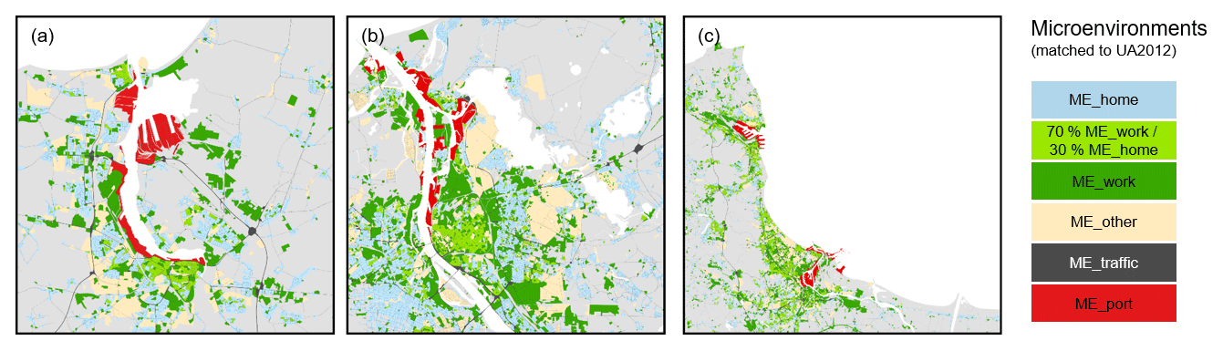
Figure 3Urban Atlas land use classifications, aggregated by colours according to microenvironment mapping presented in Table 2 for Rostock (a), Riga (b) and Gdańsk–Gdynia (c). Maps are created using © 2018 ESRI Inc. ArcGIS Pro 2.3.2.
Table 2Mapping of Urban Atlas 2012 classification with selected microenvironments and infiltration factors (IFs) for indoor–outdoor relationships in winter (September–February) and summer (March–August) months.

a Borrego et al. (2009), Baek et al. (1997), Chau et al. (2002) and Dimitroulopoulou et al. (2006). b Estimate in this study.

Figure 4Population Density per square kilometre as derived from Gallego (2010) in (a) Rostock, (b) Riga and (c) Gdańsk–Gdynia. Maps are created using © 2018 ESRI Inc. ArcGIS Pro 2.3.2.
The third step was the calculation of static population, taking into account city-specific statistics. Static population was calculated with raster data on population density using the Copernicus Corine Land Cover (CLC) inventory with values corresponding to density in inhabitants per square kilometre (Gallego, 2010; Fig. 4). The advantages of this approach are (1) a unified approach to estimate population in the total research domain and (2) the consideration of suburban and rural areas which do not only take into account the city's population but also the entire domain of interest. Besides this, a comparison of population derived from the population density grid shows good agreement with municipality population statistics of each city (Table 3), with slightly higher values for the region due to residencies surrounding the city limits.
Table 3Statistical data for 2012 to refine population distribution in the research domains.
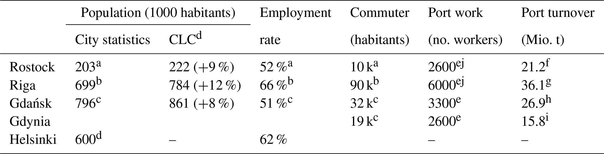
a Hanse- und Universitätsstadt Rostock. b Riga City Council Department of City Development. c Statistics Poland. d Population density disaggregated with Corine Land Cover 2000 (Gallego, 2010). e European Commission Maritime Affairs and Fisheries. f Rostock Port. g Freeport of Riga. h Port of Gdańsk, i Port Gdynia. j Own calculation.
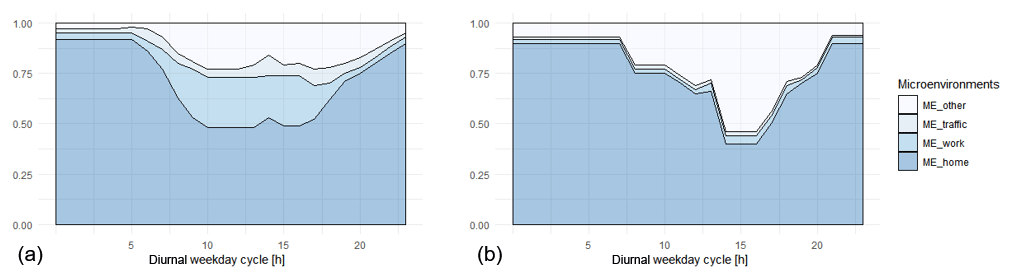
Figure 5Generic diurnal activity patterns during weekdays (a) and weekends (b), adapted from Soares et al. (2014).
In a fourth step, we assembled generic diurnal variation in population activity for each ME to temporally distribute the population to all MEs because no specific information exists for Rostock, Riga or the Gdańsk–Gdynia area. The generic time profiles are mainly derived from diurnal variation in population activity in the Helsinki metropolitan area in four MEs: home, workplace, traffic and other (Kousa et al., 2002; Soares et al., 2014). Soares et al. (2014) derived information on the Helsinki population from annually collected data of the municipalities of the Helsinki metropolitan area. We compared these with other diurnal activity patterns in Europe (Brook and King, 2017; Borrego et al., 2009) and figured out similar diurnal patterns, such as a large amount of people in the home environment during night, a growing number of people working during the day with a peak around noon followed by a decrease until early evening, and traffic rush hours in the morning and evening. Therefore, we consider the adapted pattern shown in Fig. 5 to be suitable for other Baltic Sea harbour cities. Nevertheless, we analysed the relation of employed people and the daily maximum of work activity in Helsinki to assimilate the daily maximum work activity in the generic profile for each city to account for dynamics in the second-largest ME (ME_work) and scaled all other MEs uniformly.
While we use this generic profile for weekdays, we additionally adapted a weekend profile with less work and higher other activities from the study by Borrego et al. (2009) to account for daily patterns (Fig. 5), but we did not account for holidays. Another consideration is the integration of daily commuters during workdays. We gathered data on commuting rates from the municipality of each city and assigned the total number of commuters to ME_traffic in morning and evening rush hours and ME_work during the day. When it comes to population working in the ME_port, we assigned port work as part of the ME_work, but with detailed numbers on workers in the port areas of Rostock, Riga and Gdańsk–Gdynia gathered from port-specific statistics. Therefore, we differentiate between numbers of direct port employment and indirect or related port employment to spatially distribute port workers with the UA2012 port area classification. The UA2012 classification port areas is described as the administrative area of inland harbours and seaports as well as infrastructure of port areas, including quays, dockyards, transport and storage areas, and associated areas. Thus, it is possible to use the UA2012 port area classification to distribute numbers of workers in direct port employment activities spatially. Moreover, we assumed three-shift operation in the port areas and therefore distributed the harbour workers, with 25 % belonging to the night shift, 50 % to the day shift (taking into account administrative work during day) and 25 % to the late shift. The number of harbour workers is then removed from ME_work.
Following this approach, it is possible to compile the number and spatial distributions of people for every hour of the diurnal cycle and in each defined microenvironment in the form gridded datasets. Therefore, we account for dynamics of a moving population. For this study, we generated created grids with a resolution of 100 m, following the resolution of the simulated concentration fields for NO2 and PM2.5.
We evaluate and present results for simulated concentrations in the Baltic Sea harbour cities Rostock, Riga and the urban agglomeration of Gdańsk–Gdynia, focussing on NO2. For each city, we performed runs with and without shipping to determine the effect of local shipping on NO2 concentration levels as well as population-level exposure to NO2. Besides the exposure of all ME due to total concentrations and shipping activities, we analyse the exposure to shipping-related concentrations in ME_home, ME_work and ME_port.
3.1 Evaluation of simulated concentrations
Due to an insufficient number of valid time series at the measurement stations in 2012 for Rostock and Riga to achieve significant performance indication, we focus on a discussion of measurement evaluation in the Gdańsk–Gdynia agglomeration, which contains eight valid NO2 measurement time series. In Rostock, there are four stations for NO2, while in Riga there are two stations for NO2. However, statistical indicators for NO2, O3 and PM10 for all available stations in all cities as well as a detailed description of the AQ simulation performance in Rostock and Riga can be found in Supplement Sect. SII of this paper.
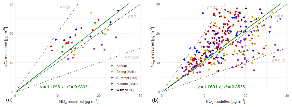
Figure 6Modelled versus measured NO2 concentrations at all available measurement stations in the Gdańsk–Gdynia research domain. Panel (a) shows annual station averages, with each dot indicating one station, while panel (b) shows daily averages, with each dot indicating an average of all stations. For panels (a) and (b) the colours display seasons.
The analysis of spatial correlations for NO2 time series in Gdańsk–Gdynia showed an r2 of 0.3 for station-averaged daily averages in 2012 and an r2 of 0.79 for station-specific annual averages (Fig. 6). The analysis of temporal correlation for hourly values over 1 year at single stations shows four urban background stations with r values between 0.3 and 0.35 and four urban background stations with r values between 0.2 and 0.3. The poorer correlation values can be expected due to non-localised information on temporal emissions. Modelled NO2 for hourly values over 1 year is in agreement with observed NO2 with overestimation of NO2 at the station Wrzeszcz (urban background station located in an urban green area; latitude 54.38028, longitude 18.62028; height 40 m a.s.l.) by 4 % and underestimation of NO2 (−1 % to −26 %) at all other (urban background) stations. NO2 shows overall good performance, and factor of two of observations (FAC2) values for NO2 in Gdańsk–Gdynia reach from 0.46–0.7 and therefore fulfil the acceptance criteria for urban regions of FAC2 ≥0.3 as defined by Hanna and Chang (2012).
3.2 Predicted concentrations and impact of shipping on NO2 in 2012
Hourly and annual NO2 concentrations at all available measurement stations throughout 2012 in all harbour cities are mostly below concentration limits as defined by the EU Air Quality Directive: while there are no exceedances for Rostock and Riga, there is only exceedance of the hourly NO2 limit of 200 µg m−3 at a station close to the port of Gdańsk. The graphical analysis of the highest annual mean NO2 concentrations in all urban domains shows three typical areas of elevated NO2 pollution levels above 20 µg m−3, which is the guideline value for annual mean concentrations defined by the WHO (2006): roads with high traffic density, city centres, port areas and areas surrounding the port areas (Fig. 7).
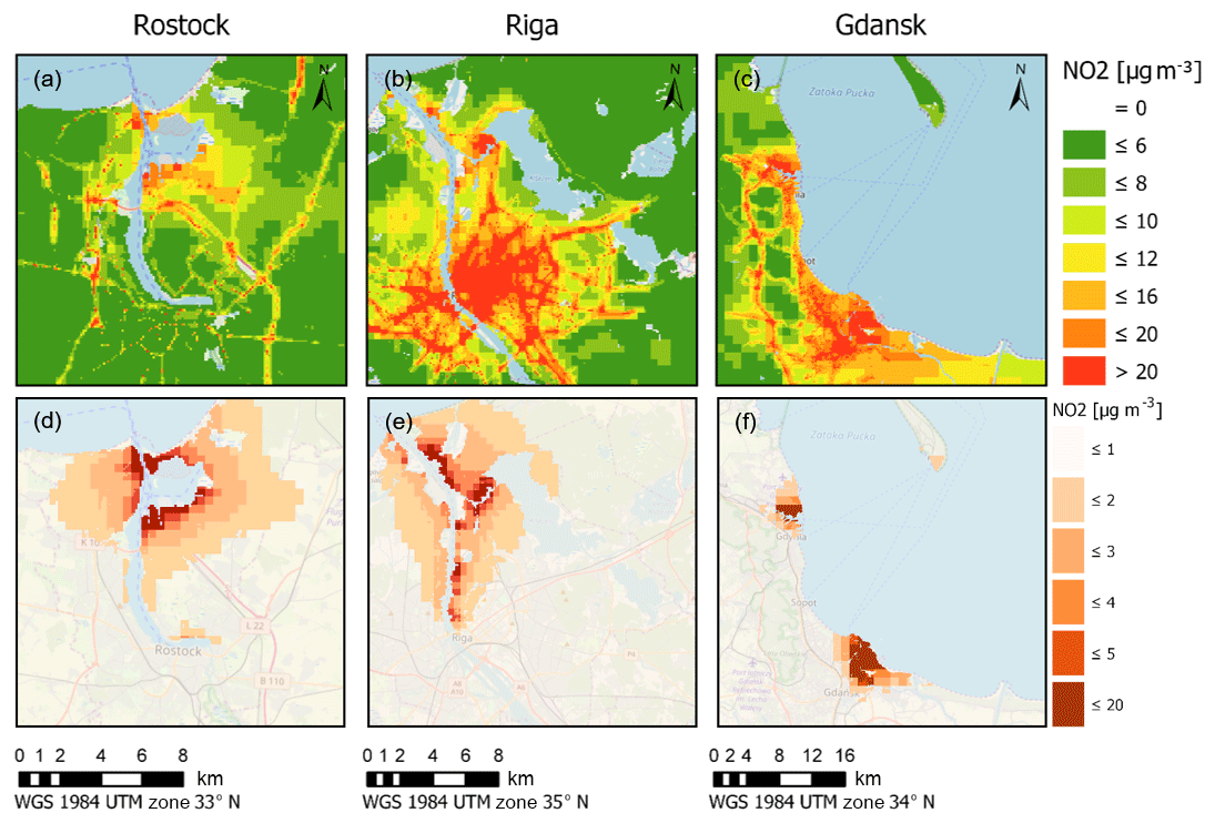
Figure 7NO2 annual mean concentrations in Rostock (a), Riga (b) and Gdańsk–Gdynia (c), and contribution of local shipping to annual mean NO2 concentration in Rostock (d), Riga (e) and Gdańsk–Gdynia (f). Maps are created using © 2018 ESRI Inc. ArcGIS Pro 2.3.2 with a topographic base map by © OpenStreetMap contributors 2019. Distributed under a Creative Commons BY-SA License.
The contribution of shipping to the NO2 concentrations (Table 4) in Rostock is significant, with a 22 % impact on the NO2 annual averaged grid mean in the complete domain. In Rostock, the shipping impact is concentrated with high values in areas inside the harbour and decreases rapidly with growing distance to the port areas. For Riga, the contribution of shipping to NO2 concentrations has a lower impact on the total annual averaged grid mean of 11 %. It is mainly located along the river Daugava, north of the main city, but also impacts areas west of the river with concentrations of 3–5 µg m−3 NO2. Comparing the spatial patterns of averaged air quality and the impact of shipping in Riga in terms of NO2, it becomes evident that areas with elevated concentration levels mostly do not overlap with areas of high NO2 concentrations due to shipping, especially in the city centre. Thus, shipping is not considered to be the main contributor to NO2 concentrations in the city centre. In Gdańsk–Gdynia, the contribution of shipping is low over land. Most of the emissions are transported seawards, leading to enhanced concentration levels in the east and northeast of the most polluted areas, which are not displayed in Fig. 7. Due to the main interest in population-level exposure to NO2 concentrations, we show concentrations only in areas with population densities above zero. Nevertheless, the port area of Gdańsk, which is located next to the city centre, shows maximum ship contributions of up to 20 µg m−3. In total, shipping contributes 16 % to the total annual averaged grid mean in the Gdańsk–Gdynia domain, whose extent (40 km × 40 km) is 4 times bigger than for Riga (20 km × 20 km). Although the average contribution of shipping to the total NO2 concentration within the entire modelled domain was modest in all urban research domains, these contributions can be higher than 20 % in the vicinity of the harbours within a distance of approximately 1 km. The total urban area impacted by emissions from shipping, determined as the area with ship-contributed NO2 concentrations above 5 µg m−3, was 5.88 km2 for Rostock, 9.26 km2 for Riga and 17.42 km2 for Gdańsk–Gdynia. In relation to the extent of the three study domains, shipping affects an area corresponding to 2.73 %, 2.76 % and 3.02 % of the populated land in Rostock, Riga and Gdańsk–Gdynia, respectively.
Table 4Summary of shipping impact on NO2 and PM2.5 concentrations as total annual averaged grid mean for the total domains in 2012.
3.3 Predicted exposure to NO2
3.3.1 Exposure in all microenvironments in 2012
The population-level exposure in Rostock, Riga and Gdańsk–Gdynia was computed based on the predicted NO2 concentrations and activities of the population in different MEs. The population data were interpolated onto a rectangular grid with a horizontal grid size of 100 m × 100 m, consistent with the pollutant surface concentration grids. The population exposure was computed for each hour of the year and separately for the selected five MEs. Population exposure is a combination of both the concentration and activity (or population density) values. The fractions of exposure to NO2 in various microenvironments of each urban domain are presented in Fig. 8. In all harbour cities, the exposure at home is responsible for most of the exposure, with contributions of 59 %, 54 % and 55 % in Rostock, Riga and Gdańsk–Gdynia respectively. In Rostock and Gdańsk–Gdynia the second-highest contributor is the ME_other, at 19 % and 24 %, while in Riga the ME_work comes second, at 19 %. Nevertheless, in Riga, the ME_other contributes 18 %, which is almost as high as ME_work. In Rostock and Gdańsk–Gdynia, ME_other contributes 13 %. While the ME_traffic in all urban domains is between 7 % and 9 %, the ME_port is below 1 %, indicating a low total exposure in the port areas.
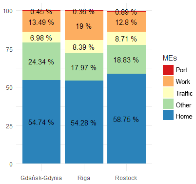
Figure 8Relative distribution of total exposure in different microenvironments based on total annual averaged grid mean exposure to NO2 in Rostock, Riga and Gdańsk–Gdynia.

Figure 9Exposure to NO2 from all sources in all microenvironments and urban domains. Maps are created using © 2018 ESRI Inc. ArcGIS Pro 2.3.2 with a topographic base map by Esri, GEBCO, NOAA, National Geographic, Garmin, HERE and other contributors.
We present the spatial distributions of the predicted annual average population exposure in Rostock, Riga and Gdańsk–Gdynia in 2012 in Fig. 9 for the total exposure and separately for all microenvironments. These distributions exhibit characteristics of both the corresponding spatial concentration distributions and population activities. There are elevated values in the city centre, along major roads and streets and in the vicinity of urban district centres. The very high home and high work exposure in the centre of Riga is caused both by the relatively high concentrations and by the highest population and workplace densities in the area. The spatial distributions of the population exposure at home and work correlate in some regions, especially in the city centres. This is due to mapping of the UA2012 category “continuous urban fabric” to ME_home and ME_work, which reflects work environments located in the city and district centres in addition to workplaces in major industrial, service and commercial regions. Nevertheless, due to less time spent being during the day in ME_work, the exposure in ME_home is higher by 1 order of magnitude. As expected, due to mapping with the UA2012 road classification, the exposure in ME_traffic is limited to the main network of roads and streets and their immediate vicinity.
3.3.2 Exposure in 2012 due to shipping
To investigate the impact of shipping on total NO2 exposure, we computed the hourly NO2 concentrations due to shipping with the ME-specific population grids of the same spatial and temporal resolution for each urban domain. The contribution of local shipping to the total population exposure as well as to the different MEs to NO2 concentrations in Rostock, Riga and Gdańsk–Gdynia are presented in Table 5. Moreover, we present in Fig. 10 the spatial distributions of annually averaged predicted population exposure to NO2 in Rostock, Riga and Gdańsk–Gdynia in 2012, which originated from shipping and in the MEs ME_home, ME_work and ME_port.
Table 5Total annual averaged grid mean exposure to NO2 due to shipping emissions in different microenvironments relative to the total annual averaged grid mean exposure to NO2 from all sources.
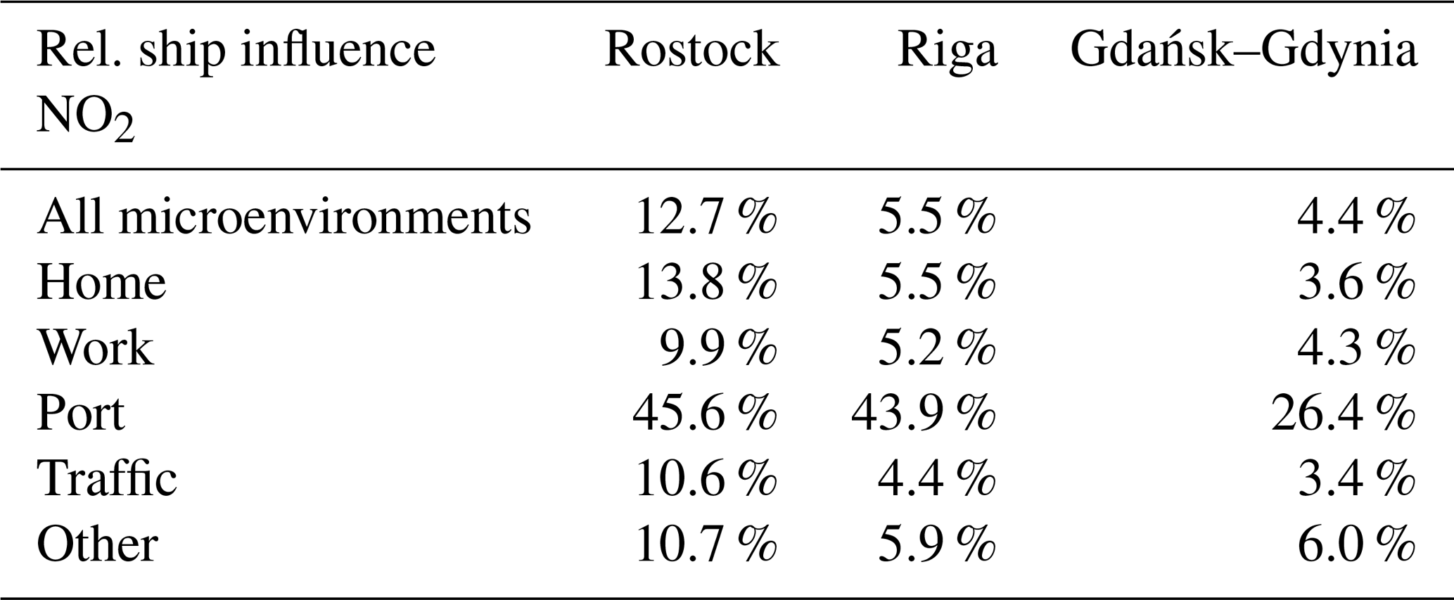
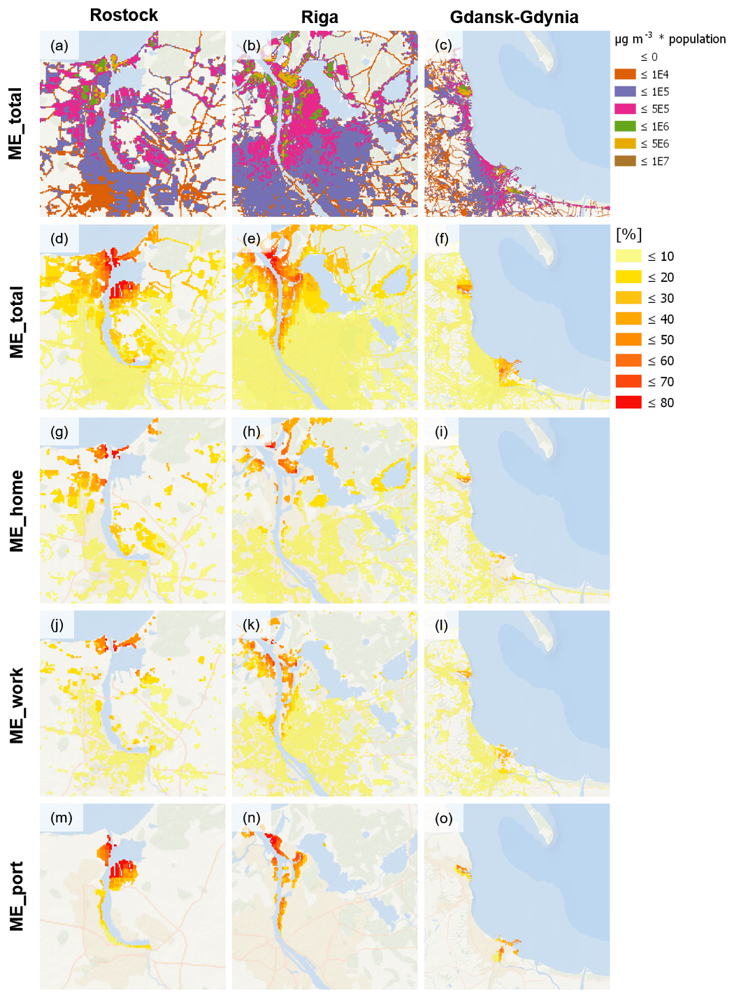
Figure 10Exposure to NO2 from local shipping as relative contribution to all microenvironments (d–f), ME_home (g–i), ME_work (j–l) and ME_port (m–o) of absolute contribution from shipping-related NO2 exposure (a–c). Maps are created using © 2018 ESRI Inc. ArcGIS Pro 2.3.2 with a topographic base map by Esri, GEBCO, NOAA, National Geographic, Garmin, HERE and other contributors.
The population exposure from local shipping in Rostock is responsible for about 13 % of the total exposure in all MEs. Thus, shipping is a substantial source of exposure to NO2 in the Rostock urban area. The biggest influence of shipping to NO2 exposure is close to the shore at the port area's exit in the south of the city, which is densely populated and a major attraction in Rostock. In this area, shipping contributes up to 80 % to the annual mean exposure. A detailed analysis of the affected MEs shows a contribution of shipping as total annual averaged grid mean to ME_home which is slightly higher (14 %) than the exposure to all MEs. Especially residencies to the north and west of the port areas show high exposure to NO2, again with relative contributions of 80 %. The microenvironment with the strongest influence due to shipping is, as expected, the ME_port, with annually averaged contributions of 46 % in the total ME_port. Thus, a reduction of shipping emissions inside the port area, e.g. with onshore power supply, could decrease exposure in the ME_port and therefore exposure to the port workers by almost the half with respect to the annual mean. In some areas of the ME_port, especially in the northern parts, the exposure due to shipping is between 50 % and 80 % compared to the total exposure from all sources. Regarding the other MEs, the contribution of shipping is about 10 %–11 % as the annually averaged grid mean, but the ME_work is also of importance in the northern areas close to the shore. In general, the population exposure caused by shipping is focussed in central Rostock, near the main harbours and within some densely inhabited parts of the city and decreases in the northern direction.
In Riga and Gdańsk–Gdynia there are similarities to Rostock regarding the decrease in shipping-emission-related exposure to NO2 with increasing distance from harbour and the importance of residencies close to the port areas. The overall contribution of shipping emissions to the total annual averaged grid mean exposure in all MEs is lower in Riga and Gdańsk–Gdynia (5 % and 4 %, respectively). In addition, the annual averaged grid mean contribution of shipping emissions to the ME_port in Riga is similar to Rostock (44 %) but lower in Gdańsk–Gdynia (26 %). Nevertheless, the absolute exposure is of the same order of magnitude in all cities. Thus, besides these gridded means, there are hotspots of the contribution from shipping in some work, port work and residential areas close to the port. In Riga, the entrance to the port and the port itself are located very close to the city centre, and some areas of the ME_work along the river Daugava are substantially exposed to NO2 from shipping, with relative contributions between 40 % and 80 %. In the Gdańsk–Gdynia study domain, most of the shipping emissions occur outside of the city on the sea, especially in the port of Gdańsk, with its main activities being located close to the sea and having predominant winds from the southwest which advect pollutants emitted from shipping away from the city centre. Nevertheless, the impact of shipping to NO2 exposure is significant close to the harbour and along the coast, especially in the populated areas in the north of Gdynia, but with less relative exposure due to shipping, at a maximum of 60 %, compared to exposure from all other sources in Rostock and Riga. Although the coastline of the Gdańsk–Gdynia domain shows high absolute exposure to NO2 (Fig. 9), shipping only shows impacts of 10 %–20 % near the coastline.
We developed a generic approach to model population activity for exposure calculations (Sect. 2.6.2) to bridge the gap between static residency population numbers and very dynamic but specific population-activity data derived from surveys or gathered with mobile devices, which were both not available in the harbour cities of this study. Thus, we used generic data, and a set of assumptions which introduces spatial and temporal uncertainties in the exposure calculation, in addition to those of the applied CTM system. Exposure is the cross-product concentrations and population density. Therefore, all uncertainties that play a role for either of them have to be considered.
In terms of uncertainties within the applied CTM system that produce concentrations, the range of uncertainty can be identified by comparisons with measurements. The evaluation of measurements (Supplement Sect. SII; Table SII-2) shows a range of −26 % to +4 % for bias in annual measured vs. modelled NO2 concentrations at different stations in Gdańsk–Gdynia. In Rostock, there are higher underestimations of −56 % to −32 %, while in Riga the range is −60 % to −4 %. High underestimations in all cities mainly occur at or near traffic stations. Matthias et al. (2018) showed that the biggest uncertainty in CTM simulations is mostly due to emission data, which are a key driver and a major source of uncertainty in atmospheric chemistry transport models. Especially in urban areas, concentrations of NOx, for example, depend linearly on the local emissions. In emissions, modelling the amount, temporal distribution and spatial distribution of emissions is often uncertain and thus has a high sensitivity. For example, non-methane volatile organic carbon (NMVOC) emissions for ships in port areas were not available as output from STEAM. This restriction led us to estimate NMVOC emissions based on the carbon monoxide (CO) emissions provided. Products of incomplete combustion, like CO and NMVOC, are difficult to estimate because these emissions are very sensitive to engine load changes, engine control (mechanics and electronics), service history and fuel injection. Very little experimental information is available concerning NMVOC emissions from modern marine engines at a sufficient level of detail, and NMVOC emission factors based on measurements performed decades ago may not represent NMVOC emissions from modern marine diesel engines accurately. The lack of detailed measurement data is probably because emission measurement standards (ISO 8178) do not require NMVOC classification but report NMVOCs as total hydrocarbons instead, which makes evaluation of NMVOC species very difficult, hindering the CTM description of secondary aerosol formation with consecutive modelling effort. Nevertheless, in this study we used a CO–NMVOC emission ratio of 1.4, which is representative of emissions from auxiliary and main engines at an engine load of 70 %–80 % (Aulinger et al., 2016), to calculate NMVOC emissions from STEAM CO emissions in Rostock, Riga and Gdańsk–Gdynia. These uncertainties in emissions will translate to uncertainties in NOx concentrations due to the chemistry of ozone, NOx and volatile organic compounds (VOCs), which represent one of the major uncertainties in the field of atmospheric chemistry, especially in urban areas (Sillman, 1999). Another example of uncertainties due to emissions is traffic emissions, which play a major role in the overall urban emissions. The exposure in the ME_traffic is very likely to be under-predicted in Rostock, and probably also in Gdańsk–Gdynia and Riga, due to the following reasons. In Rostock, the traffic emission modelling is not based on actual traffic density data but was only spatially disaggregated based on road type classification and corresponding factors, which represent a national average. While in Riga and Gdańsk–Gdynia the traffic emissions are based on traffic counts, they also do not account for all the effects of traffic congestion, slowing down of traffic in certain locations and streets and the effects of idling, and the deceleration and acceleration of vehicles. Traffic congestion can increase emissions in streets during rush hours (Gately et al., 2017; Requia et al., 2018; Smit et al., 2008). The evaluation at traffic stations has also shown that NO2 was modelled with a high negative bias, although EPISODE-CityChem was run with the activated Street-Canyon-Module and therefore included treatment for dispersion in street canyons. The ME_port shows, in all urban domains, lower exposure to NO2 compared to ME_work. This is mainly due to the detailed allocation of people directly employed by the port to the ME_port, which are distributed to the comparably large port areas.
Besides emissions, also meteorological fields and regional boundary conditions are crucial inputs for correct CTM simulations. Nevertheless, Karl et al. (2019a) proved good agreement with measurements for the regional boundary conditions as calculated with CMAQ, and the performance of the meteorological module of TAPM shows very good agreements with measurements. Therefore having correct emissions is the highest priority in terms of improving the concentrations of NO2, which then will linearly improve the results of exposure calculations.
In terms of uncertainties within the population activity, which is the second part of the cross product to calculate population exposure, there are four major factors in the developed dynamic population-activity approach that need to be considered: the size of the population, the temporal distribution of the population, the spatial distribution of the population and the application of infiltration factors for different microenvironments. In the following, these will be discussed in detail.
In this study, the population in each urban domain was derived from a population density map, valid for the European Union, instead of national or municipal population counts. This introduces biases in terms of total population numbers and the spatial distribution of people in their home environments. We have shown that the total population number derived from population density maps in this study is altered by 9 %, 12 % and 8 % for Rostock, Riga and Gdańsk–Gdynia, respectively, compared to population counts valid for the cities of interest (Table 3). Nevertheless, the advantage of this approach is the detachment from municipal boundaries or statistical zones, which are often used in population counts; these could lead to blind spots in research domains, which exceed municipal boundaries or statistical zones. A future development will be the integration of “Population estimates by Urban Atlas polygon”, which is a Copernicus Land Monitoring Service product in preparation (https://land.copernicus.eu/local/urban-atlas/population-estimates-by-urban-atlas-polygon, last access: 7 July 2019). Besides this, we uniformly distribute the derived total population with UA2012 land use classifications to spatially disaggregate the total population. A future development of this approach will be the integration of population density maps as a proxy in the distribution of population to the home environment to integrate a weighted distribution of population to the UA2012 land use classifications. This will also lead to a clearer distinction of areas which are allocated to work and home environments at the same time.
We considered the UA2012 land use classification “continuous urban fabric” for both the home and work environment to have a 30 % and 70 % share due to the description of the UA2012 classification, which includes central business districts. To check the impact of this assumption, we changed the applied split of 30 % ME_home and 70 % ME_work into two tests: (1) 50 % ME_home and 50 % ME_work and (2) 70 % ME_home and 30 % ME_work in the Gdańsk–Gdynia domain. By changing the distribution of ME_home to 50 %, the contribution of ME_home to the total annual gridded mean increases by 0.7 %, while the total annual exposure increases by 1.8 %. Changing the distribution of ME_home to 70 % increases the contribution of ME_home to the total annual gridded mean by 1.2 %, while the total annual exposure increases by 3.2 %. In the same tests, the ME_work is changed to 50 % and 30 %, which results in a decrease in the ME_work contribution to the annual grid mean by 0.3 % and 0.5 %. Therefore, we evaluate the uncertainty of the applied split of 70 % ME_work and 30 % ME_home in the UA2012 land use class “continuous urban fabric” to have limited influence on the overall exposure results. Nevertheless, due to a lack of information about specific population activity in any of the urban domains, we cannot validate our assumptions in distributing population to the MEs and the connected UA2012 land use classifications. Based on the descriptions of the UA2012 land use classifications, we matched the best-fitting microenvironments but still introduced uncertainties, e.g. in the category “Industrial, commercial, public, military and private units”, which contains not only work environments but also non-work environments, e.g. schools, universities, museums or churches. When it comes to ME_work, we also considered the UA2012 class “continuous urban fabric” to mainly constitute indoor work environments in city centres and the UA2012 classes “Industrial, commercial, public, military and private units”, “Mineral extraction and dump sites” and “Construction sites” to account for mixed indoor and outdoor work environments. In future studies, a clearer distinction of the UA2012 categories in terms of numbers of workers and indoor–outdoor classification should be done; e.g. the number of workers in the category “Mineral extraction and dump sites” could be taken from city-specific statistics, and the category could be classified as an outdoor-only environment. Besides this, we considered the amount of commuters, taken from municipal statistics, in the ME_work and ME_traffic and thus accounted for people who are additionally exposed to pollution in traffic and work environments. The consideration of commuters in Gdańsk–Gdynia leads to a 4 % higher total annual population exposure and a 20 % higher annual exposure in ME_work. For a better distribution of the ME_work and ME_ other we plan to use the “point-of-interest” feature in OSM data as a proxy in future studies, which potentially allows for a better distribution between work and other activities and the identification of very busy city centres.
Table 6Comparison of total exposure to NO2 in each city for simulations with static and dynamic population, with and without ME- and seasonal-specific IFs. The approach used in this study (dynamic activity with IF) represents the baseline (100 %). The different scenarios are compared with the total NO2 exposure for each urban domain calculated as the product of NO2 concentrations (in m−3) and the dynamic population.
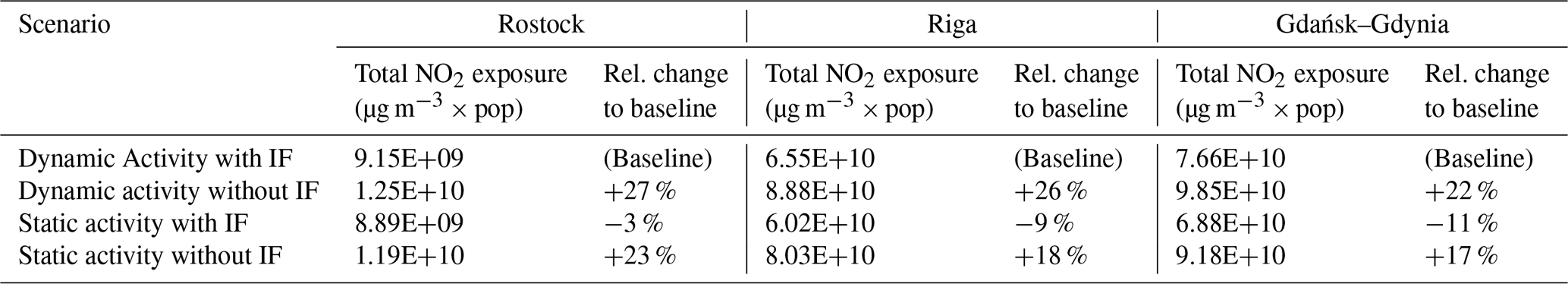
Besides uncertainties in the spatial distribution, we also introduced uncertainties regarding the temporal distribution, which is based on a temporal profile for the city of Helsinki (Soares et al., 2014). We adapted this profile and then added features which we found to appear in other European cities, such as traffic rush hours in the morning and evening. However, such a generic profile is not able to reflect the actual population activity throughout the day. Moreover, there are regional and national differences, e.g. the siesta in Mediterranean countries. Still this pattern emulates a dynamic population, which moves between environments and is exposed to different levels of pollution throughout the day. In comparison to traditional approaches, which assume people to be at their residence (home address) all the time, we believe that this approach is beneficial in particular for cities in European regions where data from surveys or positioning data from mobile devices are missing. We compared population exposure to NO2 based on our dynamic population-activity approach, with population exposure being based on a static approach to analyse the effect of a population moving in space and time on calculated population exposure. In this test, we allocated the total population all day (100 % of the time) to the home environment (ME_home) in order to simulate a static approach. The dynamic activity considers people “moving” diurnally between different MEs. Moreover, we ran simulations with and without infiltration factors to test the effect of outdoor concentrations infiltrating to indoor environments in the static and dynamic approach. The comparison between the static and the dynamic approach without the consideration of IFs (i.e. indoor air concentrations are the same as in the surrounding outdoor air) shows a decrease in total annual exposure in each city (Table 6). Therefore, the consideration of diurnal dynamic activity in different MEs leads to an increase in total population exposure. This is an effect of people moving to areas which are more polluted and, additionally, the effect of commuting inside or outside of the city.
Another assumption made in calculating exposure in different environments is the infiltration of outdoor pollutant concentrations into indoor environments. We have considered the influence of outdoor air pollution on the total population exposure. However, we have not addressed indoor sources and sinks of pollution, although indoor sources such as tobacco smoking, cooking, heating and cleaning, for example, might cause additional short-term concentration maxima in indoor environments. We have also assumed that infiltration is temporally constant, changing only with the seasons. Nevertheless, we took into account the infiltration of outdoor pollution into indoor environments (ME_work and ME_home) using IFs. To check the impact of IFs for the indoor environments, we increased and lowered the applied IFs in ME_work and ME_home in the city of Gdańsk. An increase in the IFs by 0.1 in both MEs leads to a linear increase of 10 % in ME_home and ME_work, respectively. The total exposure increases by 10 %. When it comes to the relative contribution of each ME to the total exposure, the relevance of ME_home increases to 57 % (+2.5 % points) and ME_work increases to 14 % (+0.4 % points). A similar decrease in IFs by 0.1 shows the same changes with the opposite sign. Thus, the impact of the adapted IFs on exposure in environments that are mostly indoor environments has a significant influence on the total exposure results with a linear response of the total exposure to changes of the IF. The MEs ME_other, ME_traffic and ME_ port are considered outdoor environments. When it comes to the ME_other, which is an outdoor-only environment in this study, the exposure is heavily dependent on the season due to more people spending their time outdoors in summer than in winter. This has not been considered in this study but should be taken into account in future studies. Nevertheless, the ME_other areas in the city centre are mainly green urban areas and are therefore potentially areas of high exposure in summer. In general, the applied IFs for NOx as derived from Borrego et al. (2009) represent an average of infiltration measurements in South Korea (Baek et al., 1997), Hong Kong (Chau et al., 2002) and the United Kingdom (Dimitroulopoulou et al., 2006). Thus, in future studies it is desirable to derive and use IFs, which are representative of the city-specific building infrastructure, to account for different air-intake techniques, building structures or different ventilation manners. Better parametrisation to derive more representative IFs could be derived from a combination of the EU Buildings Database, the UA2012 and climate data.
Taking into account all uncertainties and possibilities for improvement, we promote this approach for European regions in which actual data on population activity are not available, with the overall goal of improving existing exposure calculations for policy support. Nevertheless, the highest uncertainties and therefore possibilities to improve the results of the exposure calculations are as follows:
-
a better representation of emission inventories in CTM,
-
city- and microenvironment-specific infiltration factors for indoor environments,
-
city- and microenvironment-specific time profiles of population activity, and
-
city-specific spatial distribution of population in representative microenvironments.
We have presented population exposure to total and shipping-related NO2 outdoor concentrations in different microenvironments of the Baltic Sea harbour cities Rostock and Riga and the urban agglomeration of Gdańsk–Gdynia. The population exposure was calculated as a product of (1) hourly varying surface concentrations of NO2 simulated with a global-to-local chemistry transport model chain and (2) a newly developed generic approach to account for dynamic population activity in European cities.
We simulated the surface concentrations with the urban-scale CTM EPISODE-CityChem using regional boundary conditions from CMAQ simulations and land-based and ship emissions and meteorological fields for 2012 in Rostock, Riga and Gdańsk–Gdynia. The evaluation of modelled versus measured NO2 time series showed good spatial correlations and slight underestimations of annual NO2 but an overall applicable performance for studies in urban areas with a FAC2 value above 0.3 at all stations of each domain. The simulated results show the contribution of NO2 from shipping to overall air quality as being 22 % for Rostock, 11 % for Riga and 16 % for Gdańsk–Gdynia.
We developed a generic dynamic approach to account for population activity in European urban areas which is applicable for exposure calculations. Our approach aims at filling the gap between traditional approaches of exposure calculations, which are based on static population counts at residential addresses, and approaches that take into account individual activities as derived from surveys or individual GPS data. Due to missing surveys and individual GPS data in the research domains of this study, we combined existing publicly available data to follow state-of-the art exposure modelling approaches in four steps. At first, we split the total population of each urban domain into several microenvironments (home, work, traffic, other and port). Second, we distributed these microenvironments to matching land use classifications of the Urban Atlas 2012. Third, we temporally distributed the total population to the different microenvironments diurnally for weekdays and weekends, adapted from existing diurnal patterns in other European cities. Fourth, we applied infiltration factors for indoor environments to account for outdoor concentrations infiltrating indoor environments. Following this approach, it is possible to compile gridded datasets containing the number and spatial distributions of a city's population for every hour in a diurnal cycle in each defined microenvironment. For this study, we generated these grids with a grid resolution of 100 m, following the resolution of the simulated surface concentration.
In the exposure calculation, we focussed on exposure to NO2 because the ship influence was shown to be high and the regulations for NOx emission reductions will propagate slowly into the ship fleet. Moreover, NO2 from ships adds to other local sources and therefore creates problems of obeying AQ directive targets of annual mean NO2. Besides this, outdoor NO2 pollution is a health concern with lot of recent attention by the WHO.
The relative contribution of each microenvironment to total NO2 exposure is highest for the home environment, at 59 %, 54 % and 55 % in Rostock, Riga and Gdańsk–Gdynia, respectively. Although the home environment has shown that it is very sensitive to applied infiltration factors, the vast amount of people spending their time at home during the day makes the home environment the most important environment in terms of exposure to outdoor NO2. When it comes to the influence of local shipping activities, shipping contributes 13 %, 6 % and 4 % to NO2 exposure in all microenvironments in Rostock, Riga and Gdańsk–Gdynia. The shipping contribution mainly focusses on MEs near the port in all cities. MEs, which are close to the port areas, can be influenced by shipping, with up to an 80 % contribution in Rostock and Riga and up to a 50 % contribution in Gdańsk–Gdynia. The lower contributions in Gdańsk–Gdynia are due to NO2 concentrations from shipping transported towards the open sea with the predominating southwesterly winds, while in Rostock and Riga the home and work environments north of the port are mainly affected from shipping for the same reason. The differences in relative contributions from shipping are determined by the magnitude of shipping activities in relation to activities in the rest of the domain and the domain size. The contribution of shipping in the port environment is considerably higher, at 46 %, 44 % and 26 %, respectively. Nevertheless, the port environment accounts for less than 1 % of the total exposure in all domains.
In general, the applied approach for exposure modelling is capable of showing the diurnal variation in population activity and therefore diurnal exposure in different microenvironments, although we focussed on total annual population exposure in this study. By introducing dynamic population activity instead of static population activity, the total exposure in Rostock, Riga and Gdańsk increases and therefore illustrates the need for considering dynamic population activity in exposure studies. In addition, we demonstrated the importance of microenvironment- and region-specific infiltration factors in considering outdoor concentrations infiltrating indoor environments. The lack of city-specific activity profiles, workplace addresses and infiltration factors introduces the biggest uncertainties in this study. In future studies we plan to improve the spatial allocation of population by applying population density maps in the spatial disaggregation of people in the home environment and by applying OSM points of interest as well as sector statistics on workers. Therefore, a better differentiation of infiltration factors in the work environments appears to be feasible. Moreover, we plan to integrate parametrisations for infiltration factors, which will take into account public national data on building structures and building regulations as well as climate data. When it comes to the traffic environment, we also aim to integrate region-specific measurements of outdoor-to-indoor concentration ratios. Besides these efforts, further studies to test the impact of different emission sectors, such as traffic or industry, in different microenvironments are planned.
The developed approach applied for the first time for generic dynamic population activity for calculating exposure to surface concentrations is superior to traditional static approaches and can be transferred to other cities in Europe, since no need for local activity profiles is involved. Although we used a global-to-local chemistry transport model chain, the presented generic dynamic population calculation can also be used with the surface concentration field created with other methods. Therefore, we promote this approach for European regions in which specific population-activity data derived from surveys or gathered with mobile devices are not available, with the overall goal of improving existing exposure calculations for policy support and providing the basis for health effect studies.
The following datasets are available for download from the HZG FTP server upon request: (1) input data for the 1-year AQ simulations of Rostock, Riga and Gdańsk–Gdynia (full set ca. 100 GB); (2) DELTA Tool data for comparison of model output and measurements; (3) model output data of the AQ simulations of Rostock, Riga and Gdańsk–Gdynia (full set ca. 100 GB); and (4) model input and output data of the exposure calculations for all microenvironments of Rostock, Riga and Gdańsk–Gdynia (full set ca. 100 GB).
In the statistical analysis of the model performance, the following statistical indicators are used: the normalised mean bias (NMB), standard deviation (SD), root-mean-square error (RMSE), correlation coefficient (Corr), index of agreement (IOA) and the fraction of predictions within a factor of 2 of observations (FAC2). The overall bias captures the average deviations between the model and observed data, and the normalised mean bias is given by
where M and O stand for the model and observation results, respectively. The overbars indicate the time average over N time intervals (number of observations). The root-mean-square error combines the magnitudes of the errors in predictions for various times into a single measure and is defined as
where subscript i indicates the time step (time of observation values). RMSE is a measure of accuracy to compare prediction errors of different models for a particular data and not between datasets, as it is scale-dependent. The correlation coefficient (Pearson r) for the temporal correlation is defined as
including the standard deviation of model (SDM) and observation (SDO) data. The standard deviations are
The index of agreement is defined as
An IOA value close to 1 indicates agreement between modelled and observed data. The denominator in Eq. (A6) is referred to as the potential error. The fraction of modelled values within a factor of 2 (FAC2) of the observed values that the fraction of model predictions satisfy is defined as
For evaluation of modelled values in rural areas, the acceptance criteria is FAC2 ≥0.5, while in urban areas it is FAC2 ≥0.3 (Hanna and Chang, 2012). The indicator Hperc for the model capability to reproduce extreme events, e.g. exceedances, is defined as
where “perc” is the selected (high) percentile and Mperc and Operc are the modelled and observed values corresponding to the selected percentile (Thunis et al., 2012).
The supplement related to this article is available online at: https://doi.org/10.5194/acp-19-9153-2019-supplement.
MOPR created the overall structure, prepared meteorological and emission input data for the EPISODE-CityChem simulations, performed and evaluated the EPISODE-CityChem concentration simulations, developed and applied the generic dynamic activity approach, visualised and plotted all results, and wrote major parts of this publication. MK assisted with writing and discussing the overall structure, did the set-up of the EPISODE-CityChem for all domains, and programmed the preprocessing utilities. JB created land-based emissions with the SMOKE-EU model and contributed text on land-based emissions in Sect. 2.4. JPJ and LJ created local shipping emissions with STEAM and contributed text on shipping emissions in Sect. 2.5.
The authors declare that they have no conflict of interest.
This article is part of the special issue “Shipping and the Environment – From Regional to Global Perspectives (ACP/OS inter-journal SI)”. It is a result of the Shipping and the Environment – From Regional to Global Perspectives, Gothenburg, Sweden, 23–24 October 2017.
This work is part of the BONUS SHEBA (Sustainable Shipping and Environment of the Baltic Sea region) research project under call 2014-41. BONUS (Art 185) is funded jointly by the EU, Innovation Fund Denmark, Estonian Research Council, Academy of Finland, German Federal Ministry of Education and Research under grant number 03F0720A, National Centre of Research and Development (Poland), and Swedish Environmental Protection Agency.
We acknowledge Michalina Bielawska (ARMAAG), Iveta Steinberga (ELLE, University of Latvia), Stefan Nordmann and Stefan Feigenspan (UBA) for the preparation and distribution of emission datasets for Gdańsk–Gdynia, Riga and Rostock. Christane Gackenholz (former HZG) is thanked for the preparation of emission data for the UECT preprocessing utilities. Moreover, we would like to thank Stefan Seum (DLR) for traffic data from the VEU project. Copernicus Services is thanked for the public distribution of Urban Atlas and population density products. Open Street Map is thanked for maps used in plots and open source road data, which were used to distribute traffic emissions. The air quality model CMAQ is developed and maintained by the US Environmental Protection Agency (US EPA). COSMO-CLM is the community model of the German climate research. The simulations with COSMO-CLM, CMAQ and EPISODE-CityChem and the exposure calculations were performed at the German Climate Computing Centre (DKRZ) within the project “Regional Atmospheric Modelling” (project ID 0302).
The article processing charges for this open-access publication were covered by a Research Centre of the Helmholtz Association.
This paper was edited by Huan Liu and reviewed by Fabian Lenartz and one anonymous referee.
Ahas, R., Silm, S., Järv, O., Saluveer, E., and Tiru, M.: Using Mobile Positioning Data to Model Locations Meaningful to Users of Mobile Phones, J. Urban Technol., 17, 3–27, https://doi.org/10.1080/10630731003597306, 2010.
Andersson, C., Bergström, R., and Johansson, C.: Population exposure and mortality due to regional background PM in Europe – Long-term simulations of source region and shipping contributions, Atmos. Environ., 43, 3614–3620, https://doi.org/10.1016/j.atmosenv.2009.03.040, 2009.
Aulinger, A., Matthias, V., Zeretzke, M., Bieser, J., Quante, M., and Backes, A.: The impact of shipping emissions on air pollution in the greater North Sea region – Part 1: Current emissions and concentrations, Atmos. Chem. Phys., 16, 739–758, https://doi.org/10.5194/acp-16-739-2016, 2016.
Backes, A. M., Aulinger, A., Bieser, J., Matthias, V., and Quante, M.: Ammonia emissions in Europe, part II: How ammonia emission abatement strategies affect secondary aerosols, Atmos. Environ., 126, 153–161, https://doi.org/10.1016/j.atmosenv.2015.11.039, 2016.
Baek, S.-O., Kim, Y.-S., and Perry, R.: Indoor air quality in homes, offices and restaurants in Korean urban areas – indoor/outdoor relationships, Atmos. Environ., 31, 529–544, https://doi.org/10.1016/S1352-2310(96)00215-4, 1997.
Beckx, C., Int Panis, L., Arentze, T., Janssens, D., Torfs, R., Broekx, S., and Wets, G.: A dynamic activity-based population modelling approach to evaluate exposure to air pollution: Methods and application to a Dutch urban area, Environ. Impact Asses., 29, 179–185, https://doi.org/10.1016/j.eiar.2008.10.001, 2009.
Beevers, S. D., Kitwiroon, N., Williams, M. L., Kelly, F. J., Ross Anderson, H., and Carslaw, D. C.: Air pollution dispersion models for human exposure predictions in London, J. Expo. Sci. Env. Epid., 23, 647–653, https://doi.org/10.1038/jes.2013.6, 2013.
Bell, M. L.: The use of ambient air quality modeling to estimate individual and population exposure for human health research: A case study of ozone in the Northern Georgia Region of the United States, Environ. Int., 32, 586–593, https://doi.org/10.1016/j.envint.2006.01.005, 2006.
Berkowicz, R., Hertel, O., Larsen, S. E., Sorensen, N. N., and Nielsen, M.: Modelling traffic pollution in streets, available at: https://www2.dmu.dk/1_viden/2_Miljoe-tilstand/3_luft/4_spredningsmodeller/5_OSPM/5_description/ModellingTrafficPollution_report.pdf (last access: 23 January 2019), 1997.
Bieser, J., Aulinger, A., Matthias, V., Quante, M., and Builtjes, P.: SMOKE for Europe – adaptation, modification and evaluation of a comprehensive emission model for Europe, Geosci. Model Dev., 4, 47–68, https://doi.org/10.5194/gmd-4-47-2011, 2011.
Borrego, C., Sá, E., Monteiro, A., Ferreira, J., and Miranda, A. I.: Forecasting human exposure to atmospheric pollutants in Portugal – A modelling approach, Atmos. Environ., 43, 5796–5806, https://doi.org/10.1016/j.atmosenv.2009.07.049, 2009.
Brook, R. and King, K.: Updated Analysis of Air Pollution Exposure in London: Report to Greater London Authority, Oxford Centre for Innovation, Oxford, UK, 2017.
Byun, D. and Schere, K. L.: Review of the Governing Equations, Computational Algorithms, and Other Components of the Models-3 Community Multiscale Air Quality (CMAQ) Modeling System, Appl. Mech. Rev., 59, 51–77, https://doi.org/10.1115/1.2128636, 2006.
Chau, C. K., Tu, E. Y., Chan, D. W. T., and Burnett, J.: Estimating the total exposure to air pollutants for different population age groups in Hong Kong, Environ. Int., 27, 617–630, https://doi.org/10.1016/S0160-4120(01)00120-9, 2002.
Copernicus Land Monitoring Service: Urban Atlas Mapping Guide v4.7, available at: https://land.copernicus.eu/user-corner/technical-library/urban-atlas-2012-mapping-guide-new (last access: 7 July 2019), 2016.
Copernicus Land Monitoring Service: Corine Land Cover, available at: http://land.copernicus.eu/pan-european/corine-land-cover/clc-2012/ (last access: 7 July 2019), 2017.
Corbett, J. J. and Koehler, H. W.: Updated emissions from ocean shipping, J. Geophys. Res., 108, 1–13, https://doi.org/10.1029/2003JD003751, 2003.
Corbett, J. J., Fischbeck, P. S., and Pandis, S. N.: Global nitrogen and sulfur inventories for oceangoing ships, J. Geophys. Res., 104, 3457–3470, https://doi.org/10.1029/1998JD100040, 1999.
Corbett, J. J., Winebrake, J. J., Green, E. H., Kasibhatla, P., Eyring, V., and Lauer, A.: Mortality from Ship Emissions: A Global Assessment, Environ. Sci. Technol., 41, 8512–8518, https://doi.org/10.1021/es071686z, 2007.
Dalsøren, S. B., Eide, M. S., Endresen, Ø., Mjelde, A., Gravir, G., and Isaksen, I. S. A.: Update on emissions and environmental impacts from the international fleet of ships: the contribution from major ship types and ports, Atmos. Chem. Phys., 9, 2171–2194, https://doi.org/10.5194/acp-9-2171-2009, 2009.
Dewulf, B., Neutens, T., Lefebvre, W., Seynaeve, G., Vanpoucke, C., Beckx, C., and van de Weghe, N.: Dynamic assessment of exposure to air pollution using mobile phone data, Int. J. Health Geogr., 15, 1–14, https://doi.org/10.1186/s12942-016-0042-z, 2016.
Dimitroulopoulou, C., Ashmore, M. R., Hill, M. T. R., Byrne, M. A., and Kinnersley, R.: INDAIR: A probabilistic model of indoor air pollution in UK homes, Atmos. Environ., 40, 6362–6379, https://doi.org/10.1016/j.atmosenv.2006.05.047, 2006.
EC: Blue Growth – Scenarios and drivers for Sustainable Growth from the Oceans, Seas and Coasts – Third Interim Report, European Commission, Ecorys, Deltares, Oceanic Development, Rotterdam, the Netherlands/Brussels, Belgium, 2012.
EEA: The impact of international shipping on European air quality and climate forcing: EEA Technical report No 4/2013, available at: https://www.eea.europa.eu/publications/the-impact-of-international-shipping/file (last access: 11 January 2019), 2013.
EEA: Digital Elevation Model over Europe (EU-DEM v1.1), available at: https://www.eea.europa.eu/data-and-maps/data/copernicus-land-monitoring-service-eu-dem (last access: 23 January 2019), 2017.
Endresen, Ø.: Emission from international sea transportation and environmental impact, J. Geophys. Res., 108, 4560, https://doi.org/10.1029/2002JD002898, 2003.
Eyring, V., Köhler, H. W., Ardenne, J. van, and Lauer, A.: Emissions from international shipping: 1. The last 50 years, J. Geophys. Res., 110, D17305, https://doi.org/10.1029/2004JD005619, 2005.
Eyring, V., Isaksen, I. S.A., Berntsen, T., Collins, W. J., Corbett, J. J., Endresen, O., Grainger, R. G., Moldanova, J., Schlager, H., and Stevenson, D. S.: Transport impacts on atmosphere and climate: Shipping, Atmos. Environ., 44, 4735–4771, https://doi.org/10.1016/j.atmosenv.2009.04.059, 2010.
Gallego, F. J.: A population density grid of the European Union, Popul. Environ., 31, 460–473, https://doi.org/10.1007/s11111-010-0108-y, 2010.
Gately, C. K., Hutyra, L. R., Peterson, S., and Sue Wing, I.: Urban emissions hotspots: Quantifying vehicle congestion and air pollution using mobile phone GPS data, Environmental pollution (Barking, Essex 1987), 229, 496–504, https://doi.org/10.1016/j.envpol.2017.05.091, 2017.
Glasgow, M. L., Rudra, C. B., Yoo, E.-H., Demirbas, M., Merriman, J., Nayak, P., Crabtree-Ide, C., Szpiro, A. A., Rudra, A., Wactawski-Wende, J., and Mu, L.: Using smartphones to collect time-activity data for long-term personal-level air pollution exposure assessment, J. Expo. Sci. Env. Epid., 26, 356–364, https://doi.org/10.1038/jes.2014.78, 2016.
Hamer, P. D., Slørdal, L. H., Walker, S. E., Sousa-Santos, G., and Karl, M.: The urban dispersion model EPISODE. Part I: A Eulerian and sub grid-scale air quality model and its application in Nordic winter conditions, in preparation, 2019.
Hamra, G. B., Laden, F., Cohen, A. J., Raaschou-Nielsen, O., Brauer, M., and Loomis, D.: Lung Cancer and Exposure to Nitrogen Dioxide and Traffic: A Systematic Review and Meta-Analysis, Environ. Health Persp., 123, 1107–1112, https://doi.org/10.1289/ehp.1408882, 2015.
Hanna, S. and Chang, J.: Acceptance criteria for urban dispersion model evaluation, Meteorol. Atmos. Phys., 116, 133–146, https://doi.org/10.1007/s00703-011-0177-1, 2012.
Hänninen, O., Knol, A. B., Jantunen, M., Lim, T.-A., Conrad, A., Rappolder, M., Carrer, P., Fanetti, A.-C., Kim, R., Buekers, J., Torfs, R., Iavarone, I., Classen, T., Hornberg, C., and Mekel, O. C. L.: Environmental burden of disease in Europe: Assessing nine risk factors in six countries, Environ. Health Persp., 122, 439–446, https://doi.org/10.1289/ehp.1206154, 2014.
Heroux, M. E., Braubach, M., Korol, N., Krzyzanowski, M., Paunovic, E., and Zastenskaya, I.: The main conclusions about the medical aspects of air pollution: The projects REVIHAAP and HRAPIE WHO/EC, Gigiena i sanitariia, Moscow, Russia, 9–14, 2013.
Hulskotte, J. H. J. and van der Denier Gon, H. A. C.: Fuel consumption and associated emissions from seagoing ships at berth derived from an on-board survey, Atmos. Environ., 44, 1229–1236, https://doi.org/10.1016/j.atmosenv.2009.10.018, 2010.
Hurley, P. J.: TAPM: Technical description, CSIRO Marine and Atmospheric Research paper, 025, CSIRO, Aspendale, Vic., Australia, 2008.
Hurley, P. J., Physick, W. L., and Luhar, A. K.: TAPM: A practical approach to prognostic meteorological and air pollution modelling, Environ. Modell. Softw., 20, 737–752, https://doi.org/10.1016/j.envsoft.2004.04.006, 2005.
IHS: IHS Fairplay Sea-Web, Lombard House, Redhill, UK, 2017.
International Maritime Organization: Third IMO GHG Study 2014: Executive Summary and Final Report, Suffolk, UK, 2015.
Jalkanen, J.-P., Brink, A., Kalli, J., Pettersson, H., Kukkonen, J., and Stipa, T.: A modelling system for the exhaust emissions of marine traffic and its application in the Baltic Sea area, Atmos. Chem. Phys., 9, 9209–9223, https://doi.org/10.5194/acp-9-9209-2009, 2009.
Jalkanen, J.-P., Johansson, L., Kukkonen, J., Brink, A., Kalli, J., and Stipa, T.: Extension of an assessment model of ship traffic exhaust emissions for particulate matter and carbon monoxide, Atmos. Chem. Phys., 12, 2641–2659, https://doi.org/10.5194/acp-12-2641-2012, 2012.
Jiang, S., Ferreira, J., and González, M. C.: Clustering daily patterns of human activities in the city, Data Min. Knowl. Disc., 25, 478–510, https://doi.org/10.1007/s10618-012-0264-z, 2012.
Johansson, L., Jalkanen, J.-P., Kalli, J., and Kukkonen, J.: The evolution of shipping emissions and the costs of regulation changes in the northern EU area, Atmos. Chem. Phys., 13, 11375–11389, https://doi.org/10.5194/acp-13-11375-2013, 2013.
Johansson, L., Jalkanen, J.-P., and Kukkonen, J.: Global assessment of shipping emissions in 2015 on a high spatial and temporal resolution, Atmos. Environ., 167, 403–415, https://doi.org/10.1016/j.atmosenv.2017.08.042, 2017.
Karl, M. and Ramacher, M. O. P.: City-scale Chemistry Transport Model EPISODE-CityChem, Zenodo, https://doi.org/10.5281/zenodo.2158225, 2018.
Karl, M., Jonson, J. E., Uppstu, A., Aulinger, A., Prank, M., Sofiev, M., Jalkanen, J.-P., Johansson, L., Quante, M., and Matthias, V.: Effects of ship emissions on air quality in the Baltic Sea region simulated with three different chemistry transport models, Atmos. Chem. Phys., 19, 7019–7053, https://doi.org/10.5194/acp-19-7019-2019, 2019a.
Karl, M., Walker, S.-E., Solberg, S., and Ramacher, M. O. P.: The Eulerian urban dispersion model EPISODE. Part II: Extensions to the source dispersion and photochemistry for EPISODE-CityChem v1.2 and its application to the city of Hamburg, Geosci. Model Dev. Discuss., https://doi.org/10.5194/gmd-2018-325, in review, 2019b.
Karl, M., Bieser, J., Geyer, B., Matthias, V., Jalkanen, J.-P., Johansson, L., and Fridell, E.: Impact of a nitrogen emission control area (NECA) on the future air quality and nitrogen deposition to seawater in the Baltic Sea region, Atmos. Chem. Phys., 19, 1721–1752, https://doi.org/10.5194/acp-19-1721-2019, 2019c.
Kousa, A., Kukkonen, J., Karppinen, A., Aarnio, P., and Koskentalo, T.: A model for evaluating the population exposure to ambient air pollution in an urban area, Atmos. Environ., 36, 2109–2119, https://doi.org/10.1016/S1352-2310(02)00228-5, 2002.
Ledoux, F., Roche, C., Cazier, F., Beaugard, C., and Courcot, D.: Influence of ship emissions on NOx, SO2, O3 and PM concentrations in a North-Sea harbor in France, J. Environ. Sci.-China, 71, 56–66, https://doi.org/10.1016/j.jes.2018.03.030, 2018.
Leung, D. Y. C.: Outdoor-indoor air pollution in urban environment: Challenges and opportunity, Front. Environ. Sci., 2, 3579, https://doi.org/10.3389/fenvs.2014.00069, 2015.
Loyds Register Marine: Global Marine Trends 2030, available at: http://www.lr.org/en/marine/projects/global-marine-trends-2030.aspx (last access: 7 July 2019), 2014.
Matthias, V., Arndt, J. A., Aulinger, A., Bieser, J., van der Denier Gon, H., Kranenburg, R., Kuenen, J., Neumann, D., Pouliot, G., and Quante, M.: Modeling emissions for three-dimensional atmospheric chemistry transport models, J. Air Waste Manage., 68, 763–800, https://doi.org/10.1080/10962247.2018.1424057, 2018.
Merk, O.: Shipping Emissions in Ports: Discussion Paper No. 2014-20, International Transport Forum, Paris, France, 2014.
Meyer, P. de, Maes, F., and Volckaert, A.: Emissions from international shipping in the Belgian part of the North Sea and the Belgian seaports, Atmos. Environ., 42, 196–206, https://doi.org/10.1016/j.atmosenv.2007.06.059, 2008.
Neumann, B., Vafeidis, A. T., Zimmermann, J., and Nicholls, R. J.: Future coastal population growth and exposure to sea-level rise and coastal flooding – a global assessment, PloS one, 10, e0118571, https://doi.org/10.1371/journal.pone.0118571, 2015.
Nieuwstadt, F. T. M. and Meeder, J. P.: Large-Eddy Simulation of Air Pollution Dispersion: A Review, in: New tools in turbulence modelling: Les Houches School, 21–31 May 1996, edited by: Métais, O., Centre de Physique des Houches, 5, Springer, Berlin, Germanyy, 265–280, 1997.
Nyhan, M., Grauwin, S., Britter, R., Misstear, B., McNabola, A., Laden, F., Barrett, S. R. H., and Ratti, C.: “Exposure Track” – The Impact of Mobile-Device-Based Mobility Patterns on Quantifying Population Exposure to Air Pollution, Environ. Sci. Technol., 50, 9671–9681, https://doi.org/10.1021/acs.est.6b02385, 2016.
Ott, W. R.: Concepts of human exposure to air pollution, Environ. Int., 7, 179–196, https://doi.org/10.1016/0160-4120(82)90104-0, 1982.
Özkaynak, H., Baxter, L. K., Dionisio, K. L., and Burke, J.: Air pollution exposure prediction approaches used in air pollution epidemiology studies, J. Expo. Sci. Env. Epid., 23, 566–572, https://doi.org/10.1038/jes.2013.15, 2013.
Picornell, M., Ruiz, T., Borge, R., García-Albertos, P., La Paz, D. d., and Lumbreras, J.: Population dynamics based on mobile phone data to improve air pollution exposure assessments, J. Expo. Sci. Env. Epid., 1, 278–291, https://doi.org/10.1038/s41370-018-0058-5, 2019.
Pirjola, L., Pajunoja, A., Walden, J., Jalkanen, J.-P., Rönkkö, T., Kousa, A., and Koskentalo, T.: Mobile measurements of ship emissions in two harbour areas in Finland, Atmos. Meas. Tech., 7, 149–161, https://doi.org/10.5194/amt-7-149-2014, 2014.
Pregger, T. and Friedrich, R.: Effective pollutant emission heights for atmospheric transport modelling based on real-world information, Environmental pollution (Barking, Essex 1987), 157, 552–560, https://doi.org/10.1016/j.envpol.2008.09.027, 2009.
Ramacher, M. O. P., Karl, M., Aulinger, A., Bieser, J., Matthias, V., and Quante, M.: The impact of emissions from ships in ports on regional and urban scale air quality, in: Air Pollution Modeling and its Application XXV, edited by: Mensink, C. and Kallos, G., Springer Proceedings in Complexity, Springer International Publishing, Imprint, Springer, Cham, Switzerland, 309–316, 2018.
Rasche, M., Walther, M., Schiffner, R., Kroegel, N., Rupprecht, S., Schlattmann, P., Schulze, P. C., Franzke, P., Witte, O. W., Schwab, M., and Rakers, F.: Rapid increases in nitrogen oxides are associated with acute myocardial infarction: A case-crossover study, Eur. J. Prev. Cardiol., 25, 1707–1716, https://doi.org/10.1177/2047487318755804, 2018.
Reis, S., Liška, T., Vieno, M., Carnell, E. J., Beck, R., Clemens, T., Dragosits, U., Tomlinson, S. J., Leaver, D., and Heal, M. R.: The influence of residential and workday population mobility on exposure to air pollution in the UK, Environ. Int., 121, 803–813, https://doi.org/10.1016/j.envint.2018.10.005, 2018.
Requia, W. J., Higgins, C. D., Adams, M. D., Mohamed, M., and Koutrakis, P.: The health impacts of weekday traffic: A health risk assessment of PM2.5 emissions during congested periods, Environ. Int., 111, 164–176, https://doi.org/10.1016/j.envint.2017.11.025, 2018.
Rockel, B., Will, A., and Hense, A.: The Regional Climate Model COSMO-CLM (CCLM), Metz, 17, 347–348, https://doi.org/10.1127/0941-2948/2008/0309, 2008.
Saxe, H. and Larsen, T.: Air pollution from ships in three Danish ports, Atmos. Environ., 38, 4057–4067, https://doi.org/10.1016/j.atmosenv.2004.03.055, 2004.
Schneider, C., Pelzer, M., Toenges-Schuller, N., Nacken, M., and Niederau, A.: ArcGIS basierte Lösung zur detaillierten, deutschlandweiten Verteilung (Gridding) nationaler Emissionsjahreswerte auf Basis des Inventars zur Emissionsberichterstattung: Forschungskennzahl 3712 63 240 2, Texte 71/2016, Umweltbundesamt, Dessau, Germany, 2016.
Schweizer, C., Edwards, R. D., Bayer-Oglesby, L., Gauderman, W. J., Ilacqua, V., Jantunen, M. J., Lai, H. K., Nieuwenhuijsen, M., and Künzli, N.: Indoor time-microenvironment-activity patterns in seven regions of Europe, J. Expo. Sci. Env. Epid., 17, 170–181, https://doi.org/10.1038/sj.jes.7500490, 2007.
SeppȨnen, O.: Ventilation Strategies for Good Indoor Air Quality and Energy Efficiency, Int. J. Vent., 6, 297–306, 2008.
Seum, S., Heinrichs, M., Henning, A., Hepting, M., Keimel, H., Matthias, V., Müller, S., Neumann, T., Özdemir, E. D., Plohr, M., Pregger, T., Sanok, S., Sausen, R., Seebach, O., Vogel, B., and Winkler, C. (Eds.): The DLR VEU-Project Transport and the Environment – building competency for a sustainable mobility future, DLR, Berlin, Germany, 2015.
Sillman, S.: The relation between ozone, NOx and hydrocarbons in urban and polluted rural environments, Atmos. Environ., 33, 1821–1845, https://doi.org/10.1016/S1352-2310(98)00345-8, 1999.
Simpson, D., Fagerli, H., Johnson, J. E., Tsyro, S., and Wind, P.: Transboundary acidification, eutrophication and ground level ozone in Europe. Part II. Unified EMEP model performance, EMEP status report 1/2003, ISSN 0806-4520, Norwegian Meteorological Institute, Oslo, Norway, 2003.
Slørdal, L. H., Solberg, S., and Walker, S. E.: The Urban Air Dispersion Model EPISODE applied in AirQUIS2003: Technical description, NILU TR 12/2003, Norwegian Institute for Air Research, Kjeller, Norway, 2003.
Slørdal, L. H., McInnes, H., and Krognes, T.: The Air Quality Information System AirQUIS, Info. Techn. Environ. Eng, 1, 21–33, 2008.
Smit, R., Brown, A. L., and Chan, Y. C.: Do air pollution emissions and fuel consumption models for roadways include the effects of congestion in the roadway traffic flow?, Environ. Modell. Softw., 23, 1262–1270, https://doi.org/10.1016/j.envsoft.2008.03.001, 2008.
Smith, T., P. Jalkanen, J., A. Anderson, B., Corbett, J., Faber, J., Hanayama, S., O'Keeffe, E., Parker, S., Johansson, L., Aldous, L., Raucci, C., Traut, M., Ettinger, S., Nelissen, D., Lee, D., Ng, S., Agrawal, A., Winebrake, J., Hoen, M., and Pandey, A.: Third IMO GHG Study 2014: Executive Summary and Final Report, IMO, available at: http://www.imo.org/en/OurWork/Environment/PollutionPrevention/AirPollution/Documents/Third Greenhouse Gas Study/GHG3 Executive Summary and Report.pdf (last access: 7 July 2019), 2014.
Soares, J., Kousa, A., Kukkonen, J., Matilainen, L., Kangas, L., Kauhaniemi, M., Riikonen, K., Jalkanen, J.-P., Rasila, T., Hänninen, O., Koskentalo, T., Aarnio, M., Hendriks, C., and Karppinen, A.: Refinement of a model for evaluating the population exposure in an urban area, Geosci. Model Dev., 7, 1855–1872, https://doi.org/10.5194/gmd-7-1855-2014, 2014.
Sofiev, M., Kouznetsov, R., Prank, M., Soares, J., Vira, J., Tarvainen, V., and Sofieva, V.: A Long-Term Re-Analysis of Atmospheric Composition and Air Quality, in: Air Pollution Modeling and its Application XXV, edited by: Mensink, C. and Kallos, G., Springer Proceedings in Complexity, Springer International Publishing; Imprint; Springer, Cham, Switzerland, 55–59, 2018a.
Sofiev, M., Winebrake, J. J., Johansson, L., Carr, E. W., Prank, M., Soares, J., Vira, J., Kouznetsov, R., Jalkanen, J.-P., and Corbett, J. J.: Cleaner fuels for ships provide public health benefits with climate tradeoffs, Nat. Commun., 9, 406, https://doi.org/10.1038/s41467-017-02774-9, 2018b.
Sørensen, M., Loft, S., Andersen, H. V., Raaschou-Nielsen, O., Skovgaard, L. T., Knudsen, L. E., Nielsen, I. V., and Hertel, O.: Personal exposure to PM2.5, black smoke and NO2 in Copenhagen: Relationship to bedroom and outdoor concentrations covering seasonal variation, J. Expo. Sci. Env. Epid., 15, 413–422, https://doi.org/10.1038/sj.jea.7500419, 2005.
Starcrest Consulting Group, LLC: Port of Long Beach air emission inventory-2013, Long Beach, CA, USA, 2014.
Stockfelt, L., Andersson, E. M., Molnár, P., Rosengren, A., Wilhelmsen, L., Sallsten, G., and Barregard, L.: Long term effects of residential NO(x) exposure on total and cause-specific mortality and incidence of myocardial infarction in a Swedish cohort, Environ. Res., 142, 197–206, https://doi.org/10.1016/j.envres.2015.06.045, 2015.
Tang, L., Ramacher, M. O. P., Moldanova, J., Matthias, V., Karl, M., and Johansson, L.: The impact of ship emissions on air quality and human health in the Gothenburg area – Part 1: Current situtation, in preparation, 2019.
Thunis, P., Georgieva, E., and Pederzoli, A.: A tool to evaluate air quality model performances in regulatory applications, Environ. Modell. Softw., 38, 220–230, https://doi.org/10.1016/j.envsoft.2012.06.005, 2012.
Viana, M., Amato, F., Alastuey, A., Querol, X., Moreno, T., García Dos Santos, S., Herce, M. D., and Fernández-Patier, R.: Chemical Tracers of Particulate Emissions from Commercial Shipping, Environ. Sci. Technol., 43, 7472–7477, https://doi.org/10.1021/es901558t, 2009.
Viana, M., Hammingh, P., Colette, A., Querol, X., Degraeuwe, B., Vlieger, I. d., and van Aardenne, J.: Impact of maritime transport emissions on coastal air quality in Europe, Atmos. Environ., 90, 96–105, https://doi.org/10.1016/j.atmosenv.2014.03.046, 2014.
Walker, S. E.: WORM: A new open road line source model for low wind speed conditions, Int. J. Environ. Pollut., 47, 348, https://doi.org/10.1504/IJEP.2011.047348, 2011.
Walker, S. E., Solberg, S., and Denby, B.: Development and implementation of a simplified EMEP photochemistry scheme for urban areas in EPISODE: NILU TR 13/2003, NILU – Norwegian Institute for Air Research, Kjeller, Norway, 2003.
Wang, C., Corbett, J. J., and Firestone, J.: Improving Spatial Representation of Global Ship Emissions Inventories, Environ. Sci. Technol., 42, 193–199, https://doi.org/10.1021/es0700799, 2008.
WHO: Air Quality Guidelines: Global Update 2005, Particulate matter, ozone, nitrogen dioxide, and sulfur dioxide, World Health Organization, Copenhagen, Denmark, 2006.
WHO: WHO Expert Consultation: Available evidence for the future update of the WHO Global Air Quality Guidelines (AQGs): Meeting report, 29 September–1 October 2015, Bonn, Germany, 2016.
Wing, S. E., Bandoli, G., Telesca, D., Su, J. G., and Ritz, B.: Chronic exposure to inhaled, traffic-related nitrogen dioxide and a blunted cortisol response in adolescents, Environ. Res., 163, 201–207, https://doi.org/10.1016/j.envres.2018.01.011, 2018.
Xu, H., Bechle, M. J., Wang, M., Szpiro, A. A., Vedal, S., Bai, Y., and Marshall, J. D.: National PM2.5 and NO2 exposure models for China based on land use regression, satellite measurements, and universal kriging, Sci. Total Environ., 655, 423–433, https://doi.org/10.1016/j.scitotenv.2018.11.125, 2019.
- Abstract
- Introduction
- CTM and exposure simulation set-up
- Results
- Discussion of the generic exposure approach
- Conclusions
- Data availability
- Appendix A: Statistical indicators and model performance indicators
- Author contributions
- Competing interests
- Special issue statement
- Acknowledgements
- Financial support
- Review statement
- References
- Supplement