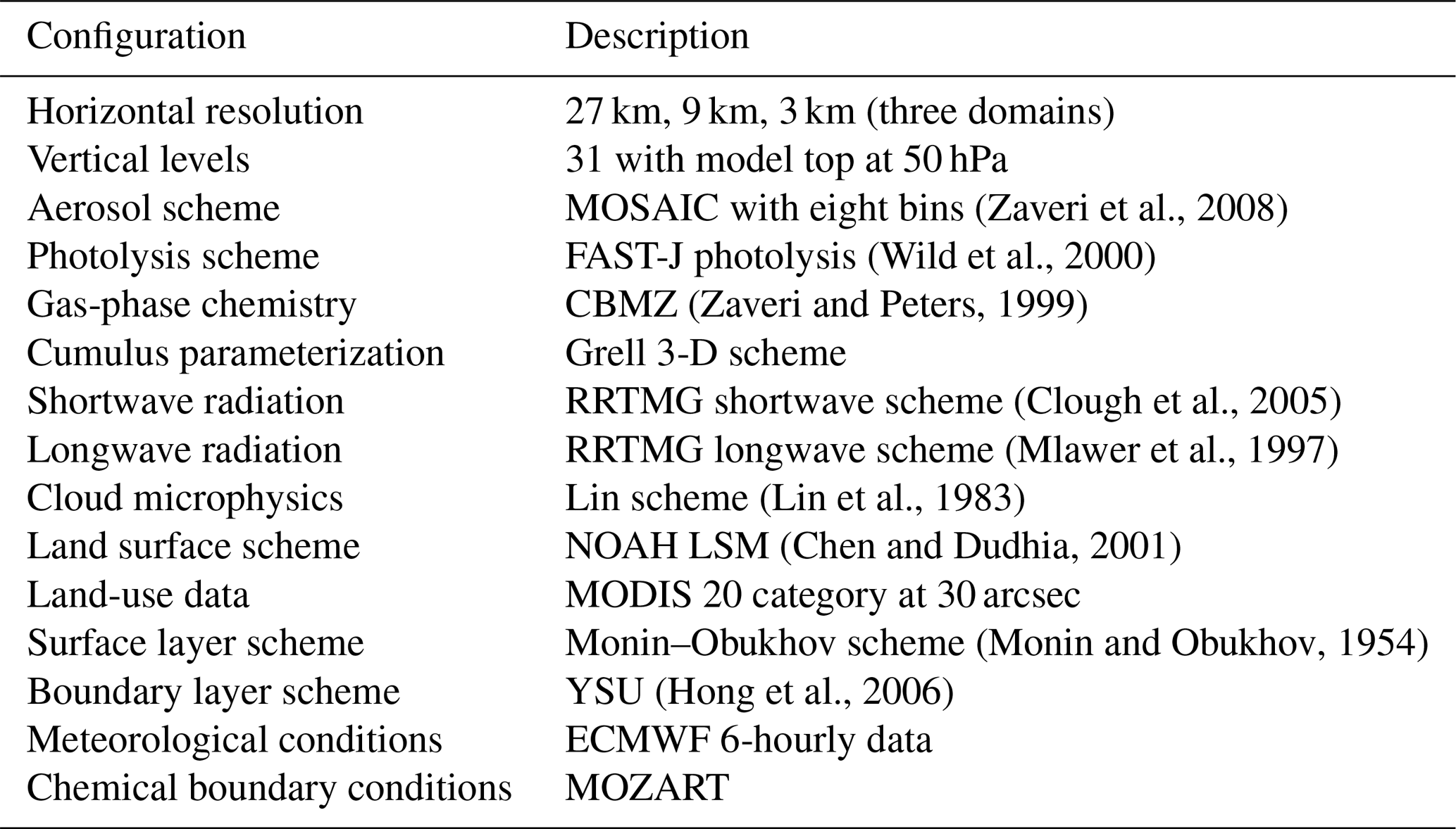
We use the WRF-Chem model (Grell et al., 2005; Fast et al., 2006) version 3.7.1 to simulate the meteorology and air quality over northern China. Previous studies have shown that WRF-Chem is capable of reproducing air quality in China relatively well (M. Gao et al., 2015, 2016; Guo et al., 2016; D. Chen et al., 2016). We use the Carbon Bond Mechanism version Z (CBMZ) chemistry scheme coupled with the Model for Simulating Aerosol Interactions and Chemistry (MOSAIC) aerosol module (Zaveri et al., 2008). CBMZ explicitly treats 67 species with 164 gas-phase, heterogeneous, and aqueous reactions and provides a suitable compromise between chemical complexity and computational efficiency. MOSAIC uses a sectional approach with eight aerosol size bins and treats the key aerosol species, including sulfate, nitrate, chloride, ammonium, sodium, black carbon, primary organic mass, liquid water, and other inorganic mass. Secondary organic aerosol (SOA) formation is not included in the chemical mechanism used here. Current SOA schemes are poorly parameterized for Chinese conditions and significantly underpredict SOA (M. Gao et al., 2016; Y. Gao et al., 2015). SOA contributed only 17 %–23 % of total ground-level fine particulate matter in Beijing during the period investigated here, while secondary inorganic aerosols contributed up to 62 % by mass (Sun et al., 2016b). We consider the lack of SOA formation in the model in drawing our conclusions. Further details of the model configuration used in this study are given in Table 1.

We perform two-way coupled simulations with three nested domains that include China as the parent domain (D01) at 27 km horizontal resolution, northern China as a nest (D02) at 9 km resolution, and the North China Plain as an innermost nest (D03) at 3 km resolution, as shown in Fig. 1. The model is nudged to meteorological reanalysis data above the boundary layer every 6 h for winds, temperature, and moisture to permit direct comparison of the simulations with observed pollutant concentrations under comparable conditions.

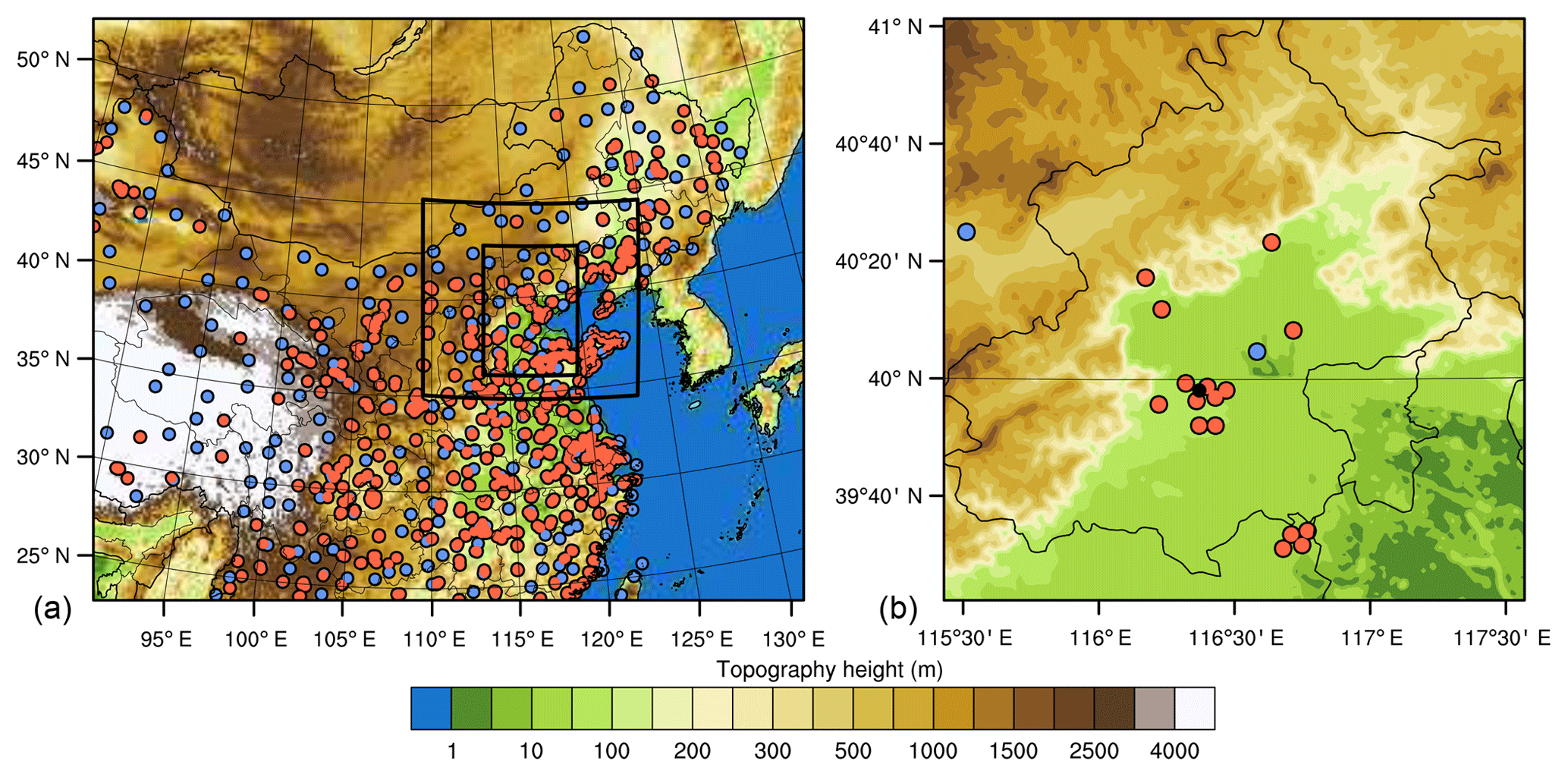
Figure 1Map of the model domain (a) showing nests over northern China and the North China Plain, and map of Beijing municipality (b) showing the location of IAP (black) and measurement stations for meteorology (blue) and air quality (red).

Download

Table 1Model configuration used in this study.

Download Print Version | Download XLSX

We use anthropogenic emissions from the Multi-resolution Emission Inventory for China (MEIC) for the year 2010 (M. Li et al., 2017). This provides emissions of major air pollutants including NO_x, CO, non-methane volatile organic compounds (NMVOCs), SO₂, NH₃, PM_2.5, PM₁₀, black carbon (BC), and organic carbon (OC) from five major emission sectors that include residential, traffic, industry, power, and agricultural sources, and it has been used in a number of previous modelling studies (Li et al., 2015; M. Gao et al., 2015; Zhang et al., 2015; H. Chen et al., 2015; D. Chen et al., 2016). Emissions were provided at the native resolution of each domain, i.e. at 27, 9, and 3 km. We impose a vertical profile for these emissions over the lowest eight model levels to account for the effective source height distribution for each sector based on the distribution used for EMEP emissions (Bieser et al., 2011; Mailler et al., 2013) and impose a diurnal cycle for each sector. SO₂ emissions over the Beijing–Tianjin–Hebei region were reduced by 50 % to account for strong emission reductions between 2010 and our focus year of 2014 (Zheng et al., 2018; Krotkov et al., 2016). We assume that 6 % by mass of SO₂ is emitted as primary SO₄ to account for the discrepancy between high observed concentrations of SO₄ and low secondary production in the model (M. Gao et al., 2015; D. Chen et al., 2016; G. Li et al., 2017). Biogenic emissions are based on the Model of Emissions of Gases and Aerosols from Nature (MEGAN; Guenther et al., 2012). These are calculated online in the model based on canopy and emission factors and factors for leaf age, soil moisture, the leaf area index, light dependence, and temperature responses. Hourly fire emissions are included from the Fire Emissions INventory from NCAR (FINN; Wiedinmyer et al., 2011) to represent biomass burning, although this is not a major source in the region at this time of year.

To evaluate the model, meteorological observations were obtained from the National Climatic Data Center (NCDC) hourly integrated surface database (http://www.ncdc.noaa.gov/data-access/, last access: 3 July 2019) for all of China. These sites are shown in Fig. 1. We focus on 2 m temperature and relative humidity, 10 m wind speed, and direction for model evaluation. Vertical profiles of meteorological variables were obtained from the 325 m high observational tower located at the Institute of Atmospheric Physics (IAP), Chinese Academy of Sciences, Beijing ($\mathrm{39}{}^{\circ }{\mathrm{58}}^{\prime }{\mathrm{28}}^{\prime \prime }$ N, $\mathrm{116}{}^{\circ }{\mathrm{22}}^{\prime }{\mathrm{16}}^{\prime \prime }$ E). This provides independent measurements of temperature, relative humidity, wind speed, and wind direction at 17 different height levels. Measurements of boundary layer mixing height were retrieved from aerosol lidar profiles at IAP (Yang et al., 2017), providing a valuable additional test of model meteorological processes. Hourly concentrations of NO₂, CO, SO₂, O₃, PM_2.5, and PM₁₀ are available from the national monitoring network run by the China National Environmental Monitoring Center (CNEMC). In addition, detailed measurements of atmospheric pollutants and aerosol composition were made from IAP tower over the October–November 2014 period. These include measurements of NH₄, NO₃, SO₄, and OC from an Aerodyne Aerosol Chemical Speciation Monitor (ACSM) instrument at 260 m altitude (Sun et al., 2016b) and from a high-resolution aerosol mass spectrometer (HR-AMS) instrument at the surface (Xu et al., 2015), and BC at the surface was measured with an aethalometer. The size-segregated samples collected at the two heights were analysed for water-soluble ions. Detailed procedures for the data analysis are described in Ng et al. (2011) and Sun et al. (2012).

To investigate the strengths and weaknesses of the model in representing air quality in China, the model was evaluated against meteorological and pollutant measurements across all three domains and at IAP tower site in Beijing.

3.1 Meteorology

We test the model performance using two sets of meteorological fields: final reanalysis data (FNL) from the National Centers for Environmental Prediction (NCEP) and ERA-Interim data from the European Centre for Medium-Range Weather Forecasts (ECMWF). Table 2 presents a comparison of the performance of the model against ground-based observations from the NCDC dataset for Beijing and the North China Plain. For a detailed evaluation over each model domain, please see Table S1 in the Supplement. The average 2 m temperature is reproduced well over the North China Plain but is overpredicted at the single Beijing site. This is located at the airport on the outskirts of the city and may not be representative of the wider region. The surface relative humidity is underpredicted for all domains with both sets of fields, although the biases are smaller and correlation is better with ECMWF data. The humidity is underpredicted by about 15 % at the Beijing site, and this may have implications for heterogeneous reactions and the hydroscopic growth of secondary aerosols. The 10 m wind speed is substantially underpredicted using both sets of fields, and this is most notable for the Beijing site. However, the correlation at this site is reasonably good, suggesting that the hourly variability in wind speeds is captured adequately. The 10 m wind direction and its variability are also reproduced relatively well. Based on these comparisons, and on subsequent comparison of pollutant concentrations, we find that the model performs marginally better using the ECMWF meteorological fields. With these fields the model captures the timing of pollution episodes better, leading to more realistic pollutant behaviour, and we have therefore chosen to use ECMWF fields for our model studies.

Table 2Comparison of observed and simulated meteorological variables using FNL and ECMWF fields.

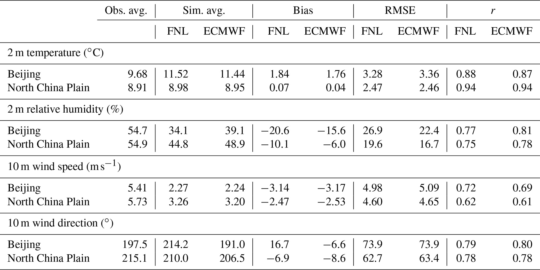
Hourly values are taken from 1 station in Beijing and 30 stations over the North China Plain from 12 October to 19 November 2014. Where observation data are missing, model values were removed to ensure that sampling was consistent.

Download Print Version | Download XLSX

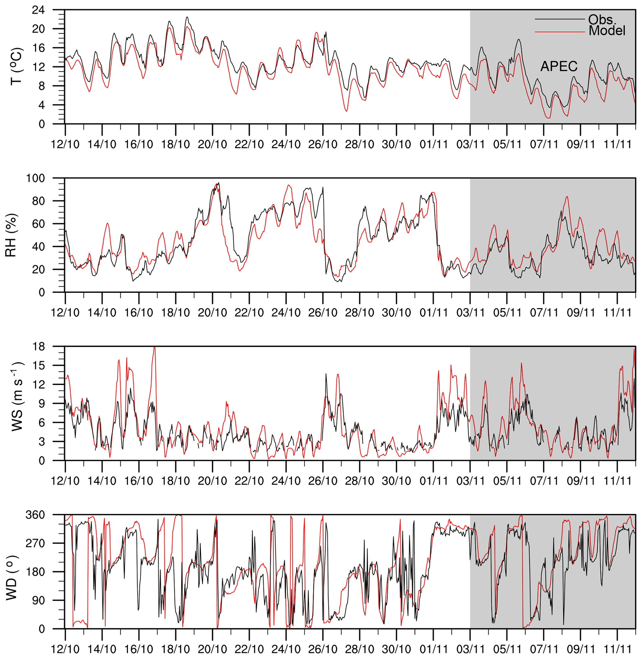
Figure 2Comparison of meteorological measurements at 190–310 m on IAP tower in Beijing with model simulations using ECMWF meteorological fields between 12 October and 12 November 2014. The period with emission controls is shaded.

Download

Figure 2 presents an evaluation of meteorological variables with measurements from IAP tower. We evaluate the model against measurements at 190–310 m (model level 4) to minimize the effects of buildings surrounding the site, which are not adequately resolved in the model. The daily maxima and minima in temperature are reproduced reasonably well, with a small underestimation that averages less than 2 ^∘C. The diurnal variations and averages for relative humidity, wind speed, and wind direction are also captured well. The mean bias in relative humidity is 0.9 %, and the large underprediction seen at the airport meteorological station is not evident here, suggesting that it may be a surface-level feature or reflect overestimation of temperature at that location. Over the height of the tower (five model levels; Fig. S2) the diurnal variation in humidity drops by more than a factor of 2, very similar to the reduction seen in the observations. The wind speed is slightly overestimated during windier periods, with a mean bias of 0.54 m s⁻¹. This suggests that the underestimation of 10 m wind speeds at meteorological stations seen in Table 2 is a surface feature in the model and does not represent a systematic bias throughout the boundary layer. The synoptic patterns in all four variables are captured very well, highlighting the quality of the ECMWF meteorological data, and there is only one occasion, on 20–21 October, when substantial deviations in temperature and humidity are evident. There are some marked differences in meteorological conditions between the APEC period (3–12 November) and the period preceding it. These include a gradual temperature drop of 7 ^∘C associated with the changing seasons, which is accompanied by a drop in relative humidity. There is an increase in the frequency of northwesterly flow with higher wind speeds, and this contrasts strongly with the lighter wind speeds and more frequent southerly flow in October. These changes are captured well by the model. A more detailed comparison of the meteorological conditions is given in Table S2 in the Supplement.

3.2 Air quality

We ran the model from 10 October to 19 November 2014 using ECMWF meteorology, and the first 2 d (days) were set aside as model spin-up. A comparison of hourly modelled pollutants for Beijing and the North China Plain against measurements from the CNEMC network is presented for October in Table 3, and the mean spatial distribution of PM_2.5 during October is shown in Fig. 3. We do not include the November period here because emission controls were implemented across Beijing and surrounding provinces from the beginning of November. A more detailed comparison of concentrations on an hourly and daily basis over all model domains is given in Table S3 in the Supplement.

Table 3Comparison of hourly pollutant concentrations with network measurements over the period 12–31 October 2014.

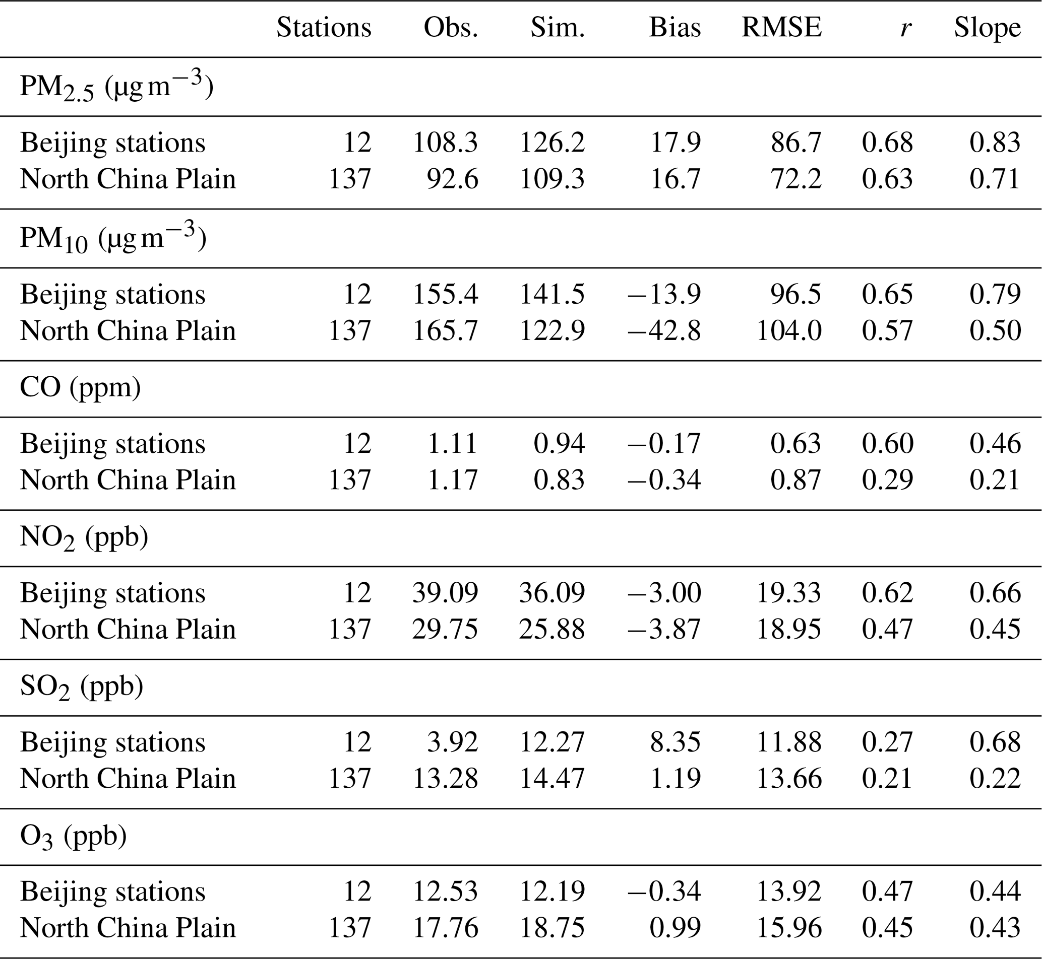
Where observation data are missing, model values were removed to ensure consistent sampling.

Download Print Version | Download XLSX

The model overpredicts average surface PM_2.5 over the period by 5 %–18 % across the three model domains. The correlation for hourly PM_2.5 improves with resolution, from r=0.47 for domain 1 to 0.63 for domain 3 and 0.68 for the 12 Beijing sites. The model underestimates PM₁₀, although the biases are relatively small (<10 %) over Beijing. This may be attributed to the lack of mineral dust sources in the model, which play a relatively small role over Beijing at this time of year. CO is underestimated over much of China, suggesting that the emissions in the inventory are too low, but the biases are relatively small over Beijing and the variability is captured well. A similar effect is seen for NO₂, which is underestimated by as much as 45 % over parts of China but by only 8 % over the Beijing sites. This may partly reflect better representation of the emission distribution for this shorter-lived pollutant on a finer grid. SO₂ is underestimated by 13 % over most of China but is overestimated over Beijing by a factor of 3. The large overestimation for Beijing can be attributed to the recent rapid reduction in emissions in the region between 2010 and 2014 that are not represented in the 2010 inventory (Zheng et al., 2018). Ozone is reproduced well over Beijing but is overestimated over much of China; this may reflect the bias in NO₂ concentrations and is likely to be influenced by the urban locations of most of the air quality stations.

For most pollutants, the correlation and slope improve substantially with resolution and are better on a daily mean basis than at hourly resolution. This suggests that the day-to-day variability driven largely by regional meteorological processes is captured better than the diurnal variations driven by chemistry and local boundary layer mixing, as expected. This is particularly noticeable for ozone, although concentrations of this pollutant remain low at this time of year. Daily mean concentrations are typically used for most metrics of pollutant impacts on human health, and the reasonable model performance for daily averaged data suggests that it is suitable for assessment of these policy-relevant metrics.

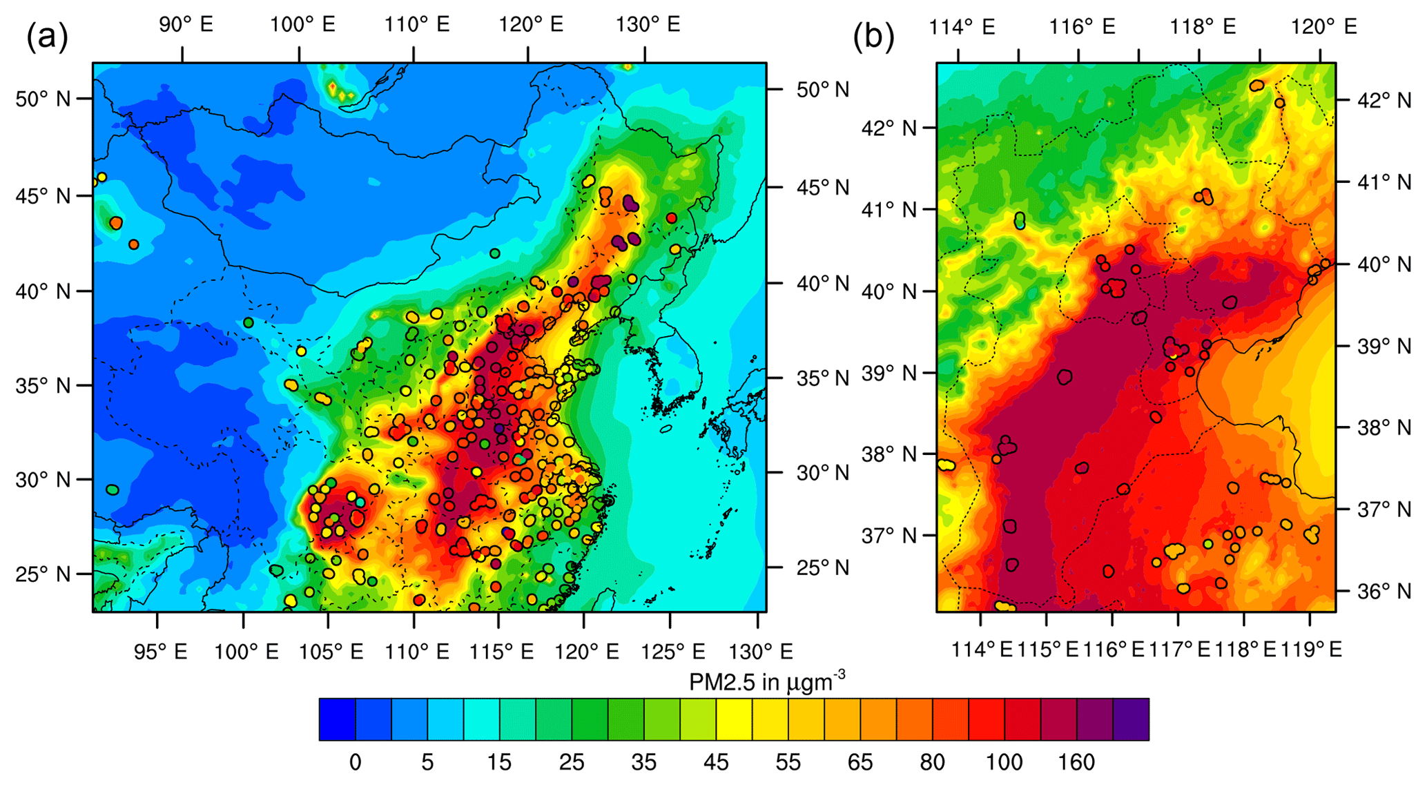
Figure 3Average spatial distribution of PM_2.5 over the period 12–31 October 2014 for model domain 1 (China; a) and domain 3 (North China Plain; b) along with observations shown in circles.

Download

The spatial distribution of mean PM_2.5 concentrations over 12–31 October is shown in Fig. 3. The distribution is captured reasonably well by the model, with the western parts of China showing clean air (with concentrations less than 10 µg m⁻³), while the eastern, more populous parts of the country show average concentrations of 70–150 µg m⁻³. Key hotspots over the North China Plain, central China, and the Sichuan Basin are reproduced, and concentrations in coastal regions are notably lower, matching observations. The North China Plain is one of the most densely populated parts of the country, incorporating major cities such as Beijing, Tianjin, and Shijiazhuang, and frequently experiences heavy haze episodes with high levels of particulate matter (Wang et al., 2014; M. Gao et al., 2015). The highest concentrations of PM_2.5 occur on the western side of the North China Plain, where they are trapped by southeasterly winds against the Taihang Mountains, and this is reproduced well by the model. There is a notable east–west gradient as concentrations drop off eastwards towards the coast. Over the mountains to the northwest of Beijing, concentrations are much lower, being typically less than 40 µg m⁻³.

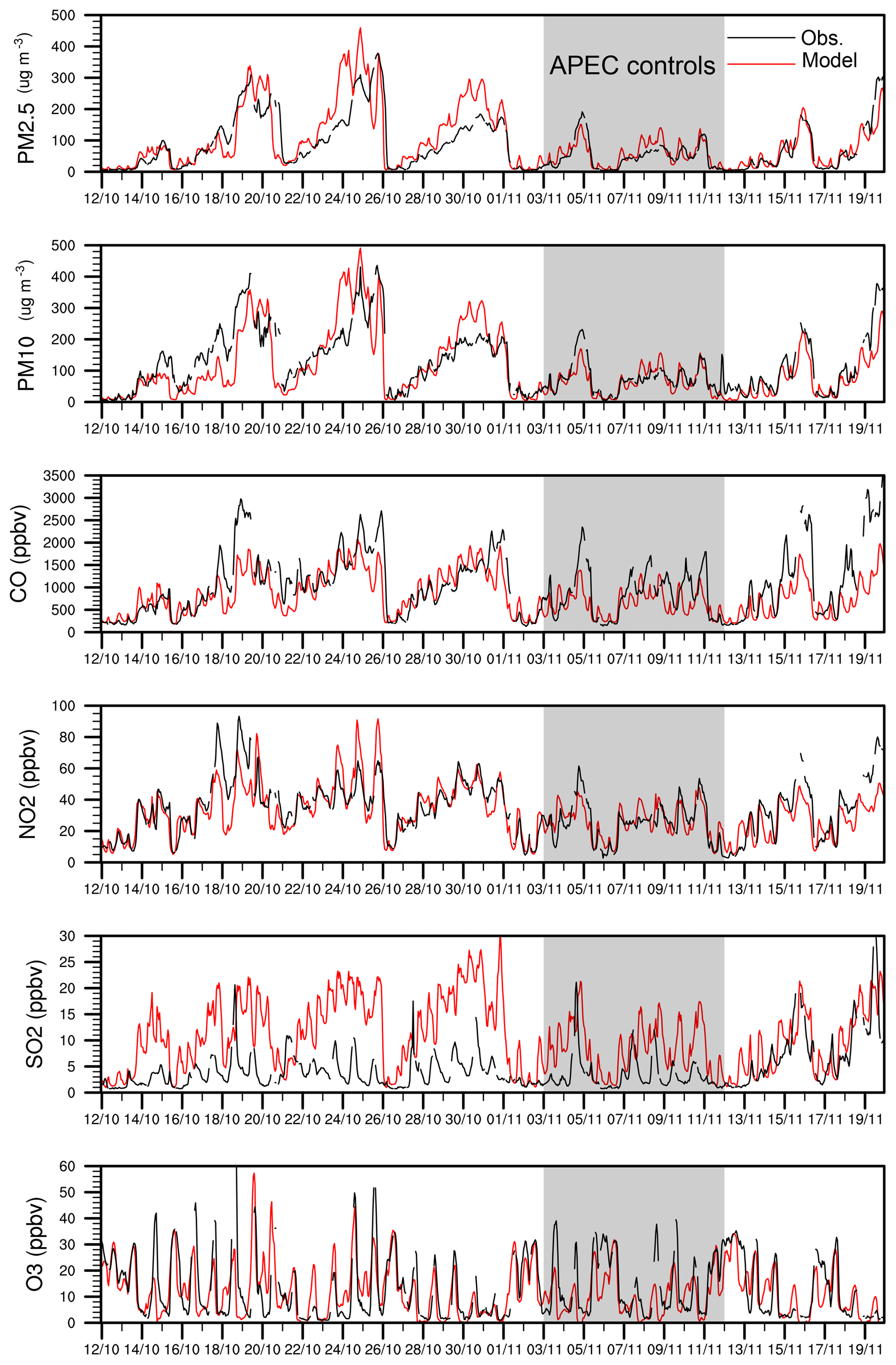
Figure 4Mean time series of surface pollutants over the 12 air quality stations in Beijing. Model values are with baseline emissions at all times, including during the APEC period (shaded).

Download

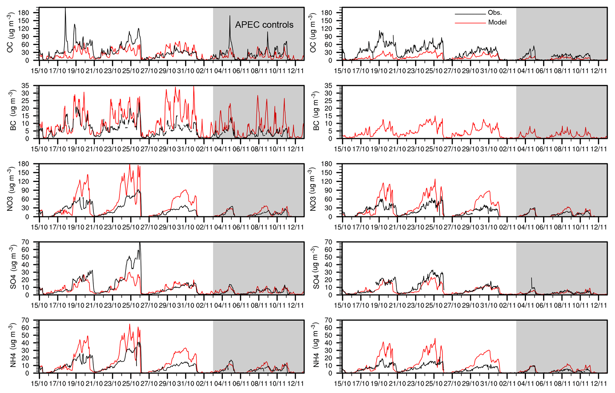
Figure 5Measured and simulated aerosol components at the surface (left) and 260 m (right) on IAP tower in Beijing. Model values are with baseline emissions at all times, including during the APEC period (shaded).

Download

Figure 4 shows the time series of key gas-phase and particulate pollutants averaged over the 12 network sites in Beijing. The general synoptic and diurnal patterns of PM_2.5, PM₁₀, CO, NO₂, and O₃ are reproduced well by the model, including the magnitude of daily maxima and minima. SO₂ is greatly overestimated in October, reflecting recent rapid emission reductions in Beijing (Zheng et al., 2018), and this is consistent with the findings of previous studies (D. Chen et al., 2016; M. Gao et al., 2015; Guo et al., 2016). However, we note that SO₂ is reproduced much better from 15 November onwards following the start of the heating season, highlighting the continuing major importance of this source. The observations show that the region experiences clear synoptic patterns of pollutant build-up over 4–5 d followed by a sudden clean-out which is typically associated with frontal passage from the northwest (Guo et al., 2014). These synoptic patterns are seen more clearly for particulate matter than for gas-phase pollutants like NO₂ and CO, which exhibit a stronger diurnal signal reflecting chemical and dynamical processes. With the exception of SO₂, key pollutants and their variation over this period are reproduced well.

Comparison of aerosol composition with measurements at IAP over this period provides a more critical test of model performance (see Fig. 5). The model overestimates BC, NO₃, and NH₄ and underpredicts OC and SO₄ during the three episodes in October. Overestimation of BC likely reflects the reduction in emissions between 2010 and 2014 but may also indicate insufficient removal in the model. The overprediction of NO₃ and NH₄ may be due to uncertainty in NO₂ and NH₃ emissions or to overestimated gas to particle conversion in the model. In particular, secondary production of NO₃ and NH₄ may be overestimated during stagnant conditions during pollution episodes but matches better in November, when conditions are less stagnant. The underestimation of SO₄ occurs despite an overestimation of gas-phase SO₂, highlighting insufficient formation of SO₄ in the model. This may also contribute to the overestimation of NO₃, as a decrease in SO₄ frees up ammonia to react with nitric acid and transfers it into the aerosol phase (Seinfeld and Pandis, 2006). The underestimation of OC can be explained by the absence of secondary organic aerosol in our studies.

The model captures the vertical gradients of NO₃ and SO₄ well, with drops of 10 %–15 % and 30 % between the surface and 260 m, respectively, similar to the drops seen in the observations. However, the model shows a weaker vertical gradient than that observed (22 % vs. 33 % drop) for NH₄, which can be attributed to higher secondary production of NH₄ in the model. For OC, the model shows a stronger vertical gradient than that observed (53 % vs. 12 % drop), which reflects the lack of secondary production at elevated levels in the model.

While the baseline model simulation with ECMWF meteorological fields reproduces observed pollutant levels reasonably well, the comparisons have highlighted uncertainties associated with resolution, vertical mixing processes, and aerosol composition. We explore the sensitivity of our results to these factors here.

4.1 Model resolution

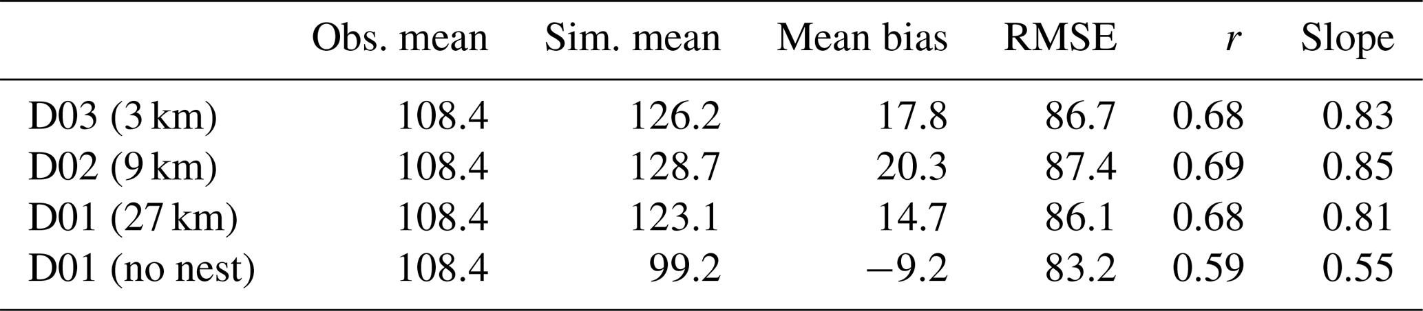
To investigate the benefits of high spatial resolution, we sample all three model domains at the 12 Beijing stations and compare the results with observations. To eliminate the influence of two-way nesting, where results from nested domains feed back to the parent domain, we perform an additional simulation at 27 km resolution over the parent domain only. Table 4 shows a comparison of modelled PM_2.5 over Beijing for the different resolutions with measurements in October. In the nested simulation, PM_2.5 is overestimated by 14 % for domain 1, 19 % for domain 2, and 16 % for domain 3 but is underestimated by 8 % for the domain 1 simulation without nesting. Although the mean biases do not improve with higher resolution, reflecting the two-way nesting, there is a substantial improvement in the correlation coefficient (0.59 to 0.68) and slope (0.55 to 0.83) for PM_2.5 when nesting is used, and this occurs for other pollutants. too (see Table S4). For many variables the results sampled at 9 km resolution (D02) are slightly better than those sampled at 3 km resolution (D03). Results at 27 km resolution without nesting are substantially less good than those with two-way nesting, highlighting the important contribution of the coupling. We conclude that it is worth performing simulations at higher horizontal resolution, as it gives a better representation of urban pollution levels.

Table 4Impacts of model resolution on simulation of hourly PM_2.5 concentrations (in µg m⁻³) in Beijing over 12–31 October 2014.

Download Print Version | Download XLSX

4.2 Boundary layer mixing

Representing turbulent mixing processes in the boundary layer well is critical for simulating surface air quality. The nighttime boundary layer under stable meteorological conditions is particularly difficult to model, and we find that the mixing height is often severely underpredicted (as low as 20 m on some occasions), causing pollutant concentrations to reach unrealistically high levels. Nudging meteorological fields to ECMWF reanalysis data reduces this bias but does not remove it. After testing a number of different boundary layer algorithms, we selected the Yonsei University (YSU) scheme (Hong et al., 2006), as it provides the best overall match to lidar-derived observations of boundary layer height. However, stable conditions remain a challenge for this scheme, and we therefore explore the sensitivity of simulated surface concentrations to boundary layer mixing under these conditions.

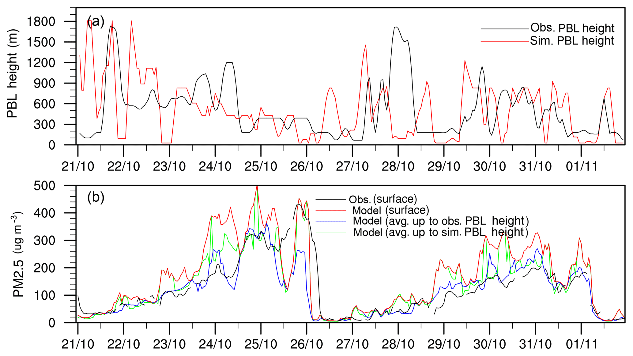
Figure 6Simulated and observed boundary layer mixing height in metres (a) and simulated and observed PM_2.5 (in µg m⁻³) showing the effect of mixing up to the PBL height in the model (b) between 21 October and 1 November 2014.

Download

Figure 6 shows the time series of simulated and observed planetary boundary layer (PBL) height. The observed PBL height was derived from lidar extinction profiles at IAP using the cubic root gradient method of Yang et al. (2017). The simulated PBL height was diagnosed using the maximum decrease in the modelled PM_2.5 profile to ensure a consistent definition. We compare the observed PBL height with the simulated height at IAP and use PM_2.5 measurements from the surface pollutant station at Aotizhongxin, the closest station to IAP site (within 2 km), to assess the effect on PM_2.5 concentrations. The PBL height shows highly variable behaviour over the day and from day to day. While the average model PBL height (514 m) is similar to the average observed height (509 m) over the haze episodes shown, the nighttime PBL height is severely underpredicted on a number of occasions. Assuming that the PBL height reflects the efficiency of mixing in the boundary layer, we expect the model to overpredict surface pollutant concentrations under these stable nighttime conditions, and this is seen in the time series of PM_2.5 in Fig. 6. To account for misrepresentation of local boundary layer mixing, we post-process the model results by vertically averaging PM_2.5 up to the simulated mixing height to eliminate the effect of underestimated mixing and up to the observed mixing height to provide a direct comparison against PM_2.5 observations. Averaging up to the observed PBL height gives a substantial improvement in PM_2.5 levels compared to observations, particularly for the episodes of 21–25 October and 27 October–1 November, when the model underestimates the PBL height. The simulated mean surface PM_2.5 concentration during the period is reduced from 169 to 118 µg m⁻³ (the observed mean is 129 µg m⁻³); the root-mean-square error (RMSE) is reduced from 94 to 65 µg m⁻³; and the biases in NO₃, NH₄, and BC are significantly reduced. For a more detailed analysis of component-level sensitivity to boundary layer mixing, see Fig. S1 and Table S5 in the Supplement.

These results highlight the importance of representing PBL mixing well for accurate reproduction of surface pollutant levels. We note a steady decline in PBL height over the pollution episode during 21–25 October, and PM_2.5 shows a consistent build-up over this period. This provides observational evidence for the radiative feedback between aerosol concentrations and mixing height, and this appears to be captured relatively well by the model, as shown in previous studies (Y. Gao et al., 2015). Further improvement in simulation of surface pollutant concentrations requires additional research on representation of PBL mixing processes in urban environments. Profiles of aerosol and meteorological variables from high-resolution lidar measurements provide an important aid to such investigations.

4.3 Regional NH₃ emissions

The aerosol components NO₃ and NH₄ are overestimated in these simulations, as shown in Fig. 5. These components are governed by secondary production from their gaseous precursors, NO₂ and NH₃. Since the concentration of NO₂ is close to that observed, we perform a short sensitivity study over the pollution episode from 21–25 October with NH₃ emissions over the North China Plain reduced by 50 % to explore the response of NO₃ and NH₄ to ammonia emissions in the model. We find that the reduction in NH₃ emissions reduces NH₄ and NO₃ concentrations substantially and brings them closer to observations (see Table 5 and Fig. S3). This is likely because NH₃ is the limiting reactant in the formation of NH₄NO₃ that directly controls the concentration of both NH₄ and NO₃ aerosols in the North China Plain (M. Gao et al., 2016; D. Chen et al., 2016). However, reduction in SO₄ concentrations is small (1 µg m⁻³) because SO₄ formation is only indirectly associated with NH₃ availability (Tsimpidi et al., 2007). Total PM_2.5 concentrations are reduced by approximately 26 %, bringing them closer to observed concentrations. Ammonia emissions were reported to be 1574 kt yr⁻¹ over the Beijing–Tianjin–Hebei region in 2010 (Zhou et al., 2015), while those in the MEIC emission inventory used here are only 540 kt yr⁻¹. Given that our NH₃ emissions are already low compared with other studies (Kang et al., 2016), we do not reduce them further in this study. However, we have demonstrated that PM_2.5 concentrations during this period are highly sensitive to NH₃ emissions, consistent with the findings of other studies (Zhang et al., 2016), and highlight this issue for further investigation.

Table 5Mean concentrations (in µg m⁻³) at IAP during 21–25 October 2014.

Download Print Version | Download XLSX

The Asia-Pacific Economic Cooperation (APEC) summit was held from 10–12 November 2014 in Beijing and was the focus of short-term emission controls to ensure good air quality over the period. Emission controls were applied in Beijing and surrounding regions, including Tianjin; the provinces of Hebei, Shanxi, and Shandong; and the Inner Mongolia autonomous region. More than 460 businesses with high emissions in Beijing were required to limit or stop their production during 3–12 November 2014 (Tang et al., 2015; H. Wang et al., 2016; Guo et al., 2016). The number of private vehicles in operation over this period was reduced by about 50 % through odd–even license-plate restrictions. Furthermore, 9300 enterprises were suspended, 3900 enterprises were ordered to limit production, and more than 40 000 construction sites were shut down across the northern China region (Y. Wang et al., 2016; Tang et al., 2015). The start-up of municipal winter heating systems was delayed until 15 November, after the summit. Previous studies report that implementation of these emission controls resulted in significant impacts on regional pollutant transport and local pollutant contributions (Meng et al., 2014; Sun et al., 2016b; Gao et al., 2017).

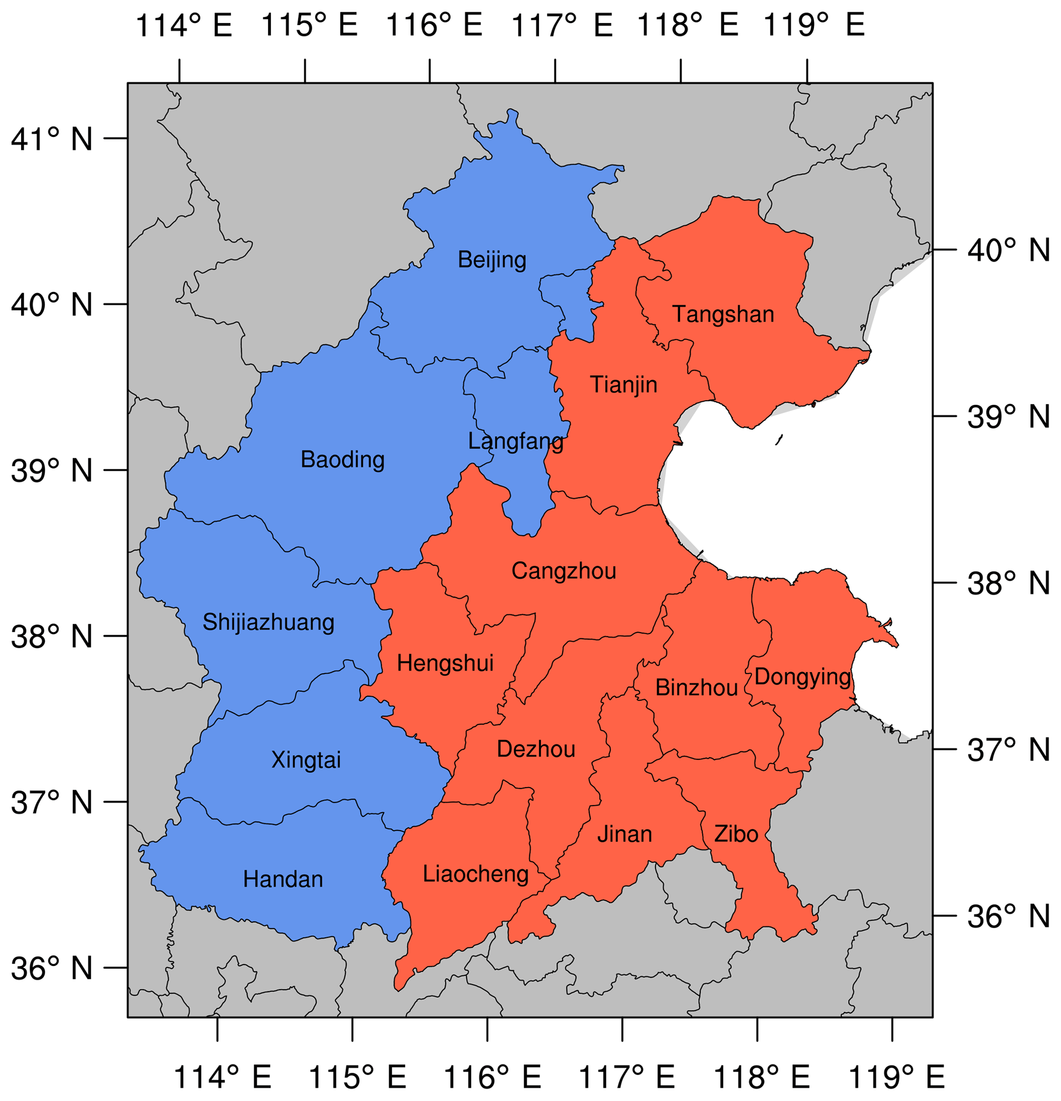
Figure 7Map of districts where major emission controls were implemented during the APEC period. During phase 1 emissions were focussed on Beijing and western Hebei (blue), and in phase 2 additional controls were applied over other parts of the North China Plain (red).

Download

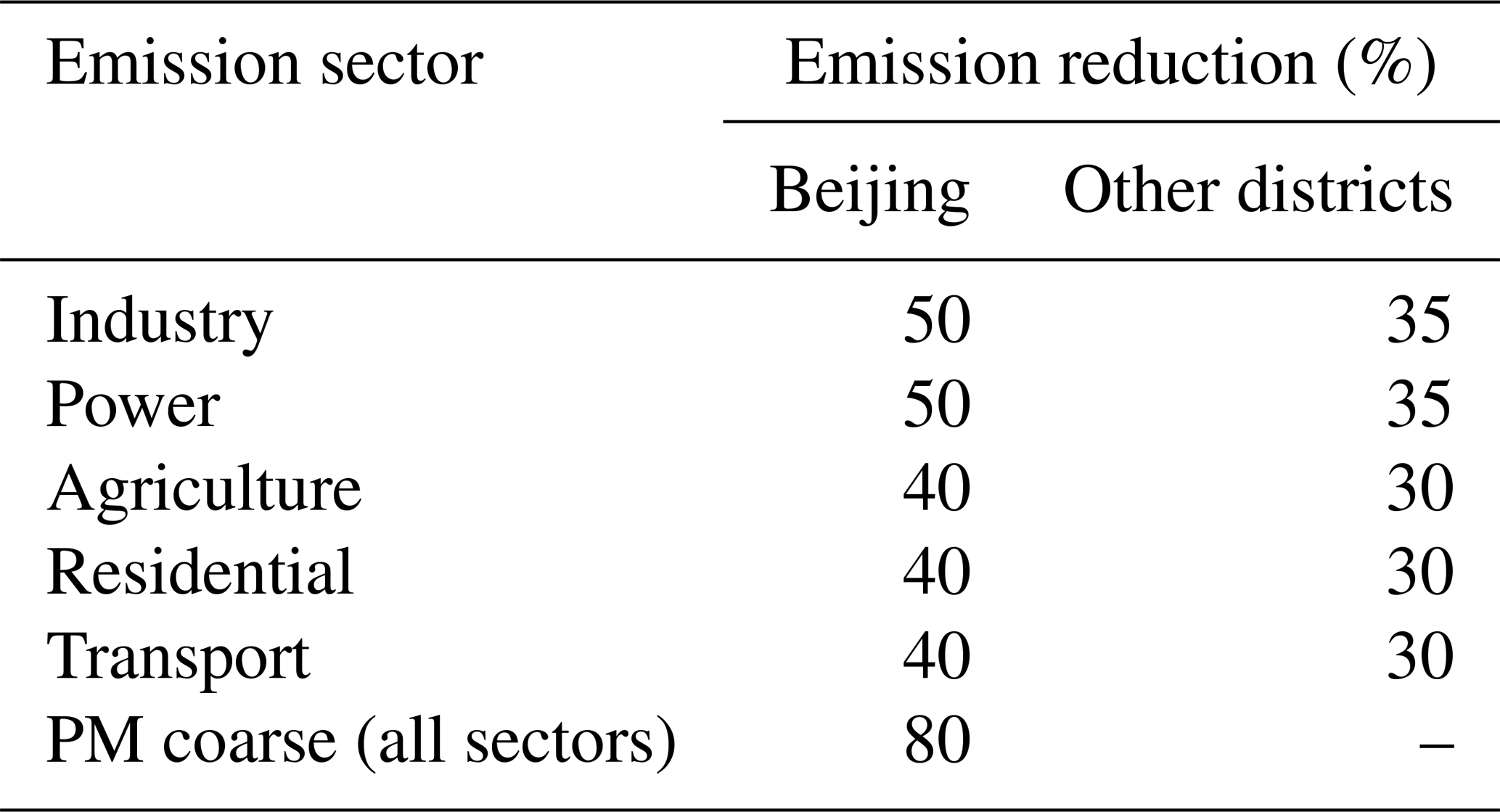
Table 6Emission controls during APEC period.

APEC1: Beijing, Langfang, Baoding, Shijiazhuang, Xingtai, and Handan. APEC2: APEC1 plus Tangshan, Tianjin, Cangzhou, Hengshui, Dezhou, Binzhou, Dongying, Zibo, Jinan, and Liaocheng.

Download Print Version | Download XLSX

Previous model studies of the APEC period have adopted different estimates of the emission reductions imposed (Guo et al., 2016; Gao et al., 2017; Wen et al., 2016; H. Liu et al., 2017; Wang et al., 2017). The most detailed study of emission reductions considered application of controls in two distinct phases (Wen et al., 2016), and we have chosen to implement these controls in our study, as the emission reductions applied are consistent with observation-based assessments of regional emission controls (K. Li et al., 2017). During the initial phase (APEC1; 3–5 November), emission controls were implemented in Beijing and the western side of the North China Plain. In a subsequent phase (APEC2; 6–12 November), controls were applied over a wider region including eastern Hebei and parts of Shandong. We represent these controls in the model over the districts shown in Fig. 7, following K. Li et al. (2017), and neglect smaller changes in emissions in other districts and more distant provinces. Controls were applied across different activity sectors, following Wen et al. (2016) and (K. Li et al., 2017; see Table 6).

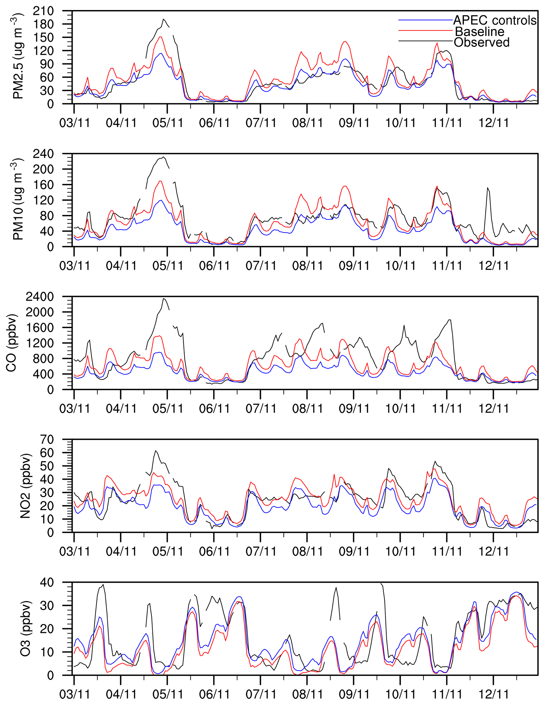
Figure 8Time series of surface pollutants averaged over the 12 measurement stations in Beijing during the APEC period.

Download

Figure 8 shows the effect of these controls on key pollutants over the period 3–12 November. There is a minor pollution episode over 4–5 November, and the model underestimates PM_2.5 levels over this period, even without emission controls. This may partly reflect an underestimation of OC, as the simulation of secondary inorganic aerosol for these 2 d is good (see Fig. 5). PM_2.5 levels are very well matched in the period 6–9 November leading up to the summit, when emission controls are applied. PM₁₀ levels are underestimated in the simulations, but this is influenced by what may be a minor dust episode on 11–12 November, when coarse particles were high but PM_2.5 remained very low. Overall, the controls had a notable effect, reducing concentrations by 20 %–30 % for all pollutants except O₃, which showed a small increase as expected with reduced levels of NO. Over the critical 10–12 November meeting period, PM_2.5, PM₁₀, CO, and NO₂ were reduced by 21 %, 26 %, 22 %, and 22 %, respectively (see Table 7). The reduction in PM_2.5 is very similar to the 22 % reduction found in previous studies (Gao et al., 2017). However, the absolute improvement in air quality over the meeting period was small, averaging less than 10 µg m⁻³ for PM_2.5 and reflecting the relatively clean conditions over the period. Average PM_2.5 in the baseline simulation was 39 µg m⁻³, close to the observed 36 µg m⁻³. Under these conditions the key air quality standard, a 24 h averaged PM_2.5 of 75 µg m⁻³, corresponding to a Chinese Air Quality Index (AQI) value of 100, would have been met in the model simulation even without the controls.

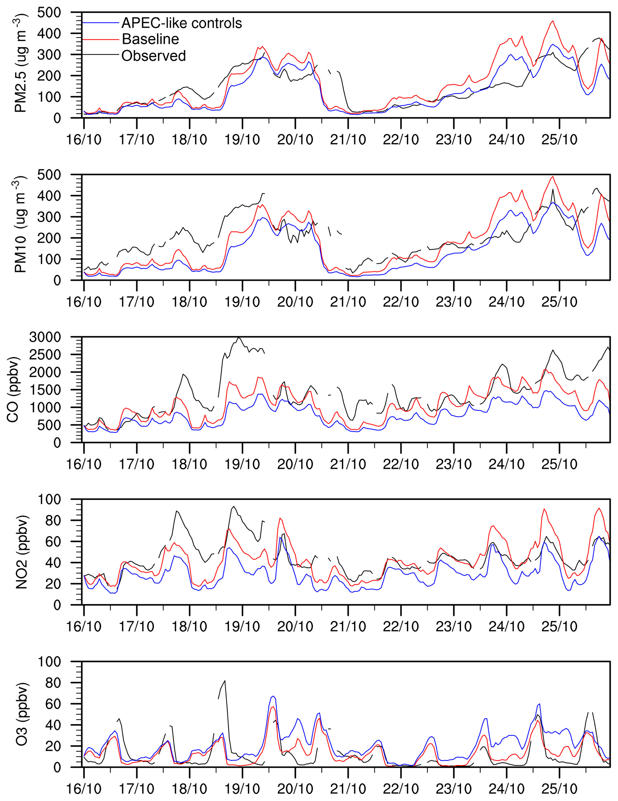
Figure 9Time series of surface pollutants averaged over the 12 measurement stations in Beijing during 16–25 October 2014.

Download

To explore the importance of meteorological conditions in contributing to favourable air quality during the APEC period, we apply the same magnitude, location, and duration of emission controls to the major pollution episode at the end of October. Figure 9 shows the effect of these controls on key pollutants over 16–25 October. The controls reduced pollutant concentrations by a larger amount than during the APEC period, but the relative improvements of 23 %–38 % were very similar. The absolute pollutant concentrations were much higher than in November. This can be attributed to lower wind speeds and to winds from the south and east bringing air from across the North China Plain, in contrast to the APEC period, which experienced higher wind speeds and more frequent air from the clean northwest sector (see Fig. 2). The 3 d baseline average concentrations over 23–25 October for PM_2.5, PM₁₀, CO, and NO₂ were 279 µg m⁻³, 310 µg m⁻³, 1.48 ppm, and 53 ppb, respectively, substantially exceeding air quality standards. The difference in baseline PM_2.5 concentrations between the October and November periods without emission controls, 279 vs. 39 µg m⁻³, highlights the dominant role played by meteorology in bringing clean air during APEC. The emission controls have a much larger absolute effect during the October episode than in the APEC period, with reductions in PM_2.5 of 65 µg m⁻³ for 23–25 October, bringing average PM_2.5 levels down to 214 µg m⁻³. However, this is insufficient in meeting the standard needed for clean air of 75 µg m⁻³. This indicates that the same emission control policies applied would have failed to produce the desired results if the meeting had been held at the end of October.

Table 8 presents the effect on aerosol components and gas-phase pollutants at IAP tower. During the emission controls in both the polluted October and cleaner November periods, primary components were reduced by 31 %–34 %, while secondary components were reduced by only 3 %–17 %. This suggests that pollution episodes dominated by primary aerosols may be more easily controlled and have serious implications for winter haze episodes over the North China Plain because much of the increase in aerosol loading is contributed by regional secondary aerosols (see Sun et al., 2016b). The percentage reduction in SO₄ (14 %–17 %) may be overestimated, as some fraction of SO₄ mass for which chemical formation pathway remains unknown is treated as primary aerosol in the model. Similarly, the percentage reduction in OC may be overestimated because all OC is primary in the model.

To investigate the feasibility of meeting air quality standards during pollution episodes such as those on 21–25 October, we ran the model with all anthropogenic emissions removed over the North China Plain from 16–25 October. The 3 d average concentrations over 23–25 October showed substantial reductions: 83 % for PM_2.5, 82 % for PM₁₀, 79 % for CO, 99 % for NO₂, and 88 % for SO₂. Average PM_2.5 concentrations were reduced from 279 to 48 µg m⁻³, demonstrating that air quality standards can be met on highly polluted days, at least in theory, under the most stringent emission controls. From this simulation, and accounting for nonlinearity in secondary aerosol formation, we estimate that a 92 % emission reduction over the 10 d period would have been needed to keep the average concentrations for 23–25 October below 75 µg m⁻³. Even accounting for model overestimation of average PM_2.5 during this period, driven principally by the positive bias on 24 October, we find that an 85 % emission reduction would be required, which is substantially more than what is feasible realistically. It is clear from this analysis that emission controls would need to be applied over a much wider area over neighbouring provinces if the air quality standards in Beijing are to be met.

Finally, we analyse the full simulation period (12 October–19 November) to investigate how many days would meet the “blue-sky” criteria of 24 h average PM_2.5 concentrations less than 75 µg m⁻³ with and without APEC-like controls. We conducted another simulation with APEC 2 controls implemented over the full period and found a reduction in daily average PM_2.5 of 26 %±6 % and a reduction of 23 %±4 % for haze days with the daily mean ${\mathrm{PM}}_{\mathrm{2.5}}>\mathrm{75}\mathrm{\mu }\mathrm{g}{\mathrm{m}}^{-\mathrm{3}}$. Since primary and secondary aerosol components can respond differently to emission controls, we use component-level fractional reductions from the model and apply them to the observed component concentrations to find the reduction in total PM. This is approximately 22 % for both October and November periods based on our APEC control runs, suggesting that this scaling is appropriate and robust for uncertainties in model aerosol composition. To generate an emission control scenario over the full period, we reduce daily mean observed PM_2.5 concentrations by 22 % for all days except 3–12 November, when controls were actually in place. For the 3–12 November period, we apply an increase of 16 %–33 % based on the APEC controls run to represent conditions with no controls. With these scenarios we find that 15 of the 39 d considered failed to meet the blue-sky criteria of daily average PM_2.5 concentrations less than 75 µg m⁻³ without controls, and this fell to 13 d when the controls were implemented, a modest decrease of 2 d (see Fig. 10). However, if we choose a higher threshold of 150 µg m⁻³ (AQI of 200), the emission controls appear to be more effective, reducing the number of exceedances from 8 to 5 d, and with a threshold of 200 µg m⁻³ (AQI of 250), the number of exceedances falls from 4 to 1 d.

Figure 10Frequency distribution of daily average PM_2.5 over 12 October–19 November 2014, showing the number of days meeting thresholds of 75 µg m⁻³ (blue) and 150 µg m⁻³ (blue plus orange) without (a) and with (b) emission controls.

Download

To organize a 3 d meeting such as APEC successfully, all 3 d must individually meet the chosen air quality criteria. We find that without emission controls, only 9 out of 37 possible 3 d time slots in our simulation period meet the criteria, including only 3 out of the 8 available during the APEC period of 3–12 November. Under the emission controls, the meeting could have been organized in 14 out of the 37 slots, including all 8 during early November. This suggests that the emission controls were only sufficient to provide an additional five time slots to hold a 3 d event meeting the criteria. Interestingly, these all occur during the APEC period, highlighting that while favourable weather conditions were vital for meeting the air quality criteria, the emission controls provided critical support in achieving the 75 µg m⁻³ threshold needed to realize blue-sky conditions. Specifically, in the absence of emission controls the first day of the APEC meeting (10 November) would have exceeded the air quality standards. In this respect, it is reasonable to claim that the APEC emission controls were a success. However, it is clear that favourable meteorology was essential in making it possible for the emission controls to produce the marginal improvements needed to meet the air quality standards.

It should be noted that 23 out of the 37 possible 3 d time periods (more than 60 %) would not have met the standards even under the emission controls applied. It is therefore clear that much more stringent controls are needed in future to counter the effect of unfavourable meteorological conditions. While greater reductions in the magnitude of emissions are required, it is important that these are applied over a much larger area, including in the neighbouring provinces that surround the North China Plain.

Table 7Influence of emission controls averaged over Beijing air quality stations in October and November.

Download Print Version | Download XLSX

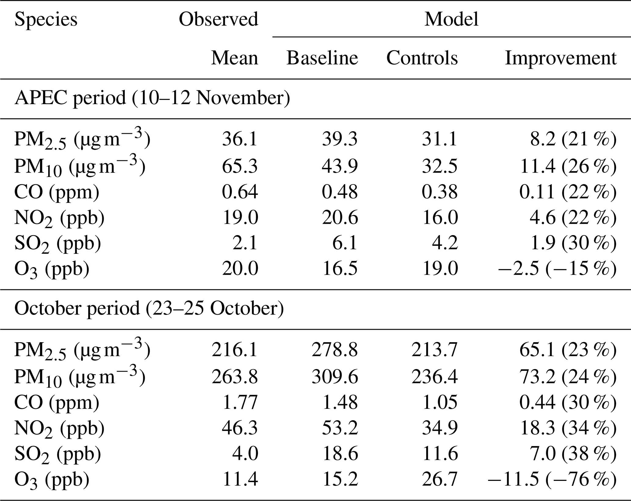
Table 8Influence of emission controls at IAP site in October and November.

Download Print Version | Download XLSX

The WRF-Chem code is available from http://www2.mmm.ucar.edu/wrf/users/download/ (Skamarock et al., 2008). The name list for the model and surface pollutant distributions generated in this study are available from the Lancaster University data archive at https://doi.org/10.17635/lancaster/researchdata/300 (Ansari, 2019).

The supplement related to this article is available online at: https://doi.org/10.5194/acp-19-8651-2019-supplement.

TUA, OW, and ZW designed this study, and TUA performed the model simulations and analysis. JL provided emission data and expertise on the model set-up; TY provided the lidar data and guidance on deriving PBL height; and YS, WX, and ZW provided measurement data from IAP tower. TUA and OW prepared the paper, with input from all co-authors.

The authors declare that they have no conflict of interest.

This research has been supported by the Natural Environment Research Council (grant nos. NE/N006925/1 and NE/N006976/1), the National Natural Science Foundation of China (grant nos. 91744207, 41571130034 and 91744203), and the Strategic Priority Research Program of the Chinese Academy of Sciences (grant no. XDA19040203).

This paper was edited by Andreas Hofzumahaus and reviewed by two anonymous referees.