2.1 WRF-Chem configuration

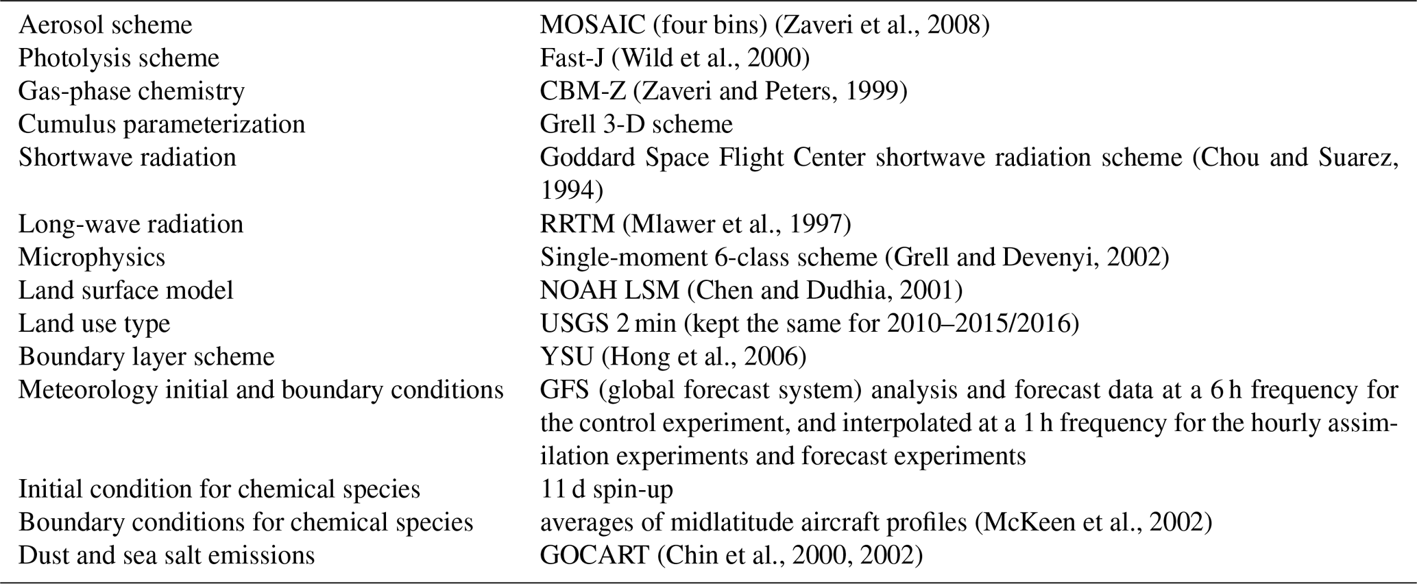
WRF-Chem model version 3.6.1 was used in this study (Grell et al., 2005; Fast et al., 2006). The parameterizations were identical to those of Chen et al. (2016), and they are listed in Table 1. The model horizontal resolution is 40 km, and the domain covers most of China and the surrounding regions (Fig. 2). There are 57 vertical levels extending from the surface to 10 hPa. It should be noted that uncertainties might be produced in the analysis due to neglecting the rapid urbanization/land use changes from 2010 to 2015/2016.

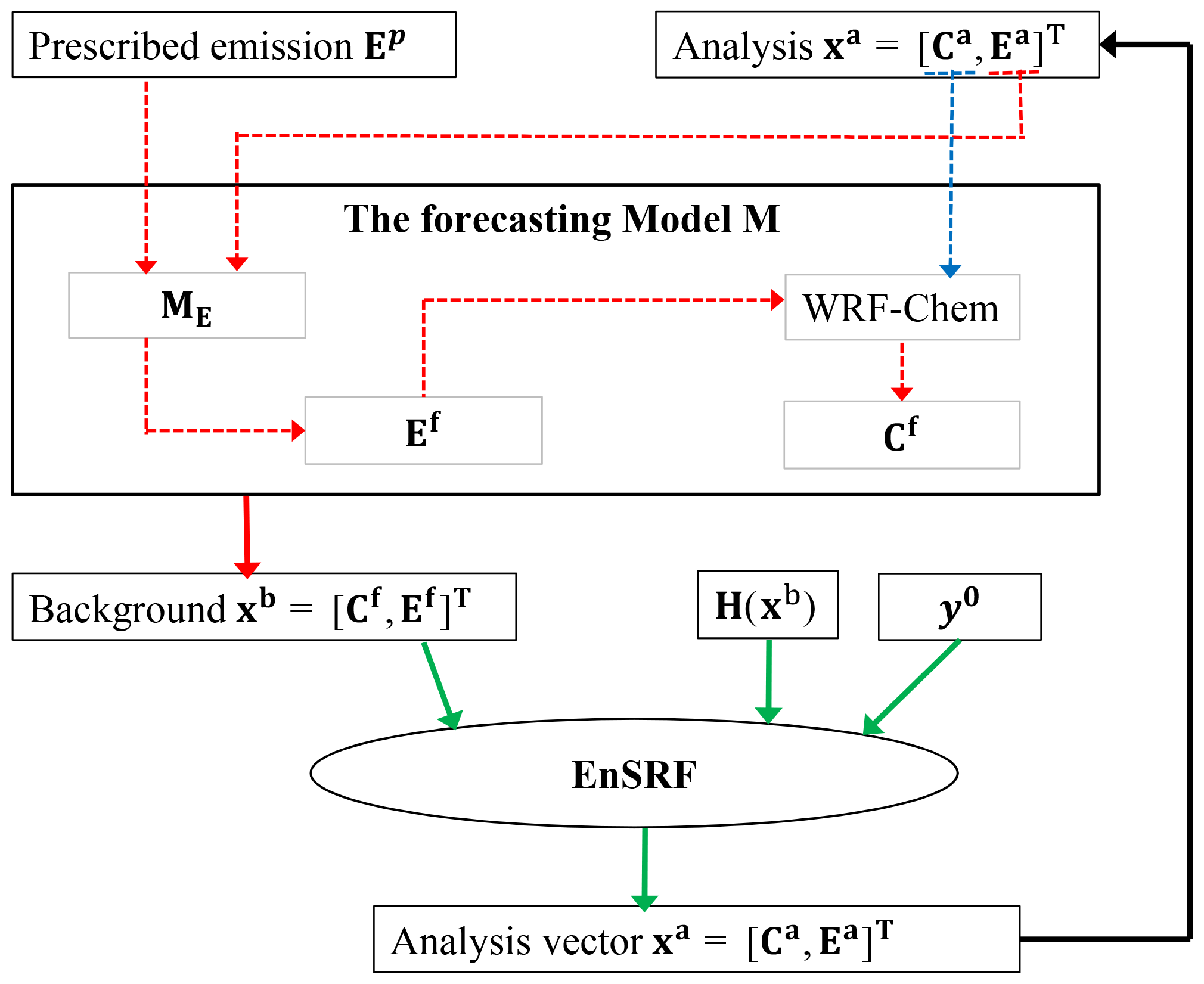
Figure 1Flow chart of the data assimilation system that simultaneously optimizes the initial chemical conditions and emissions.

Download

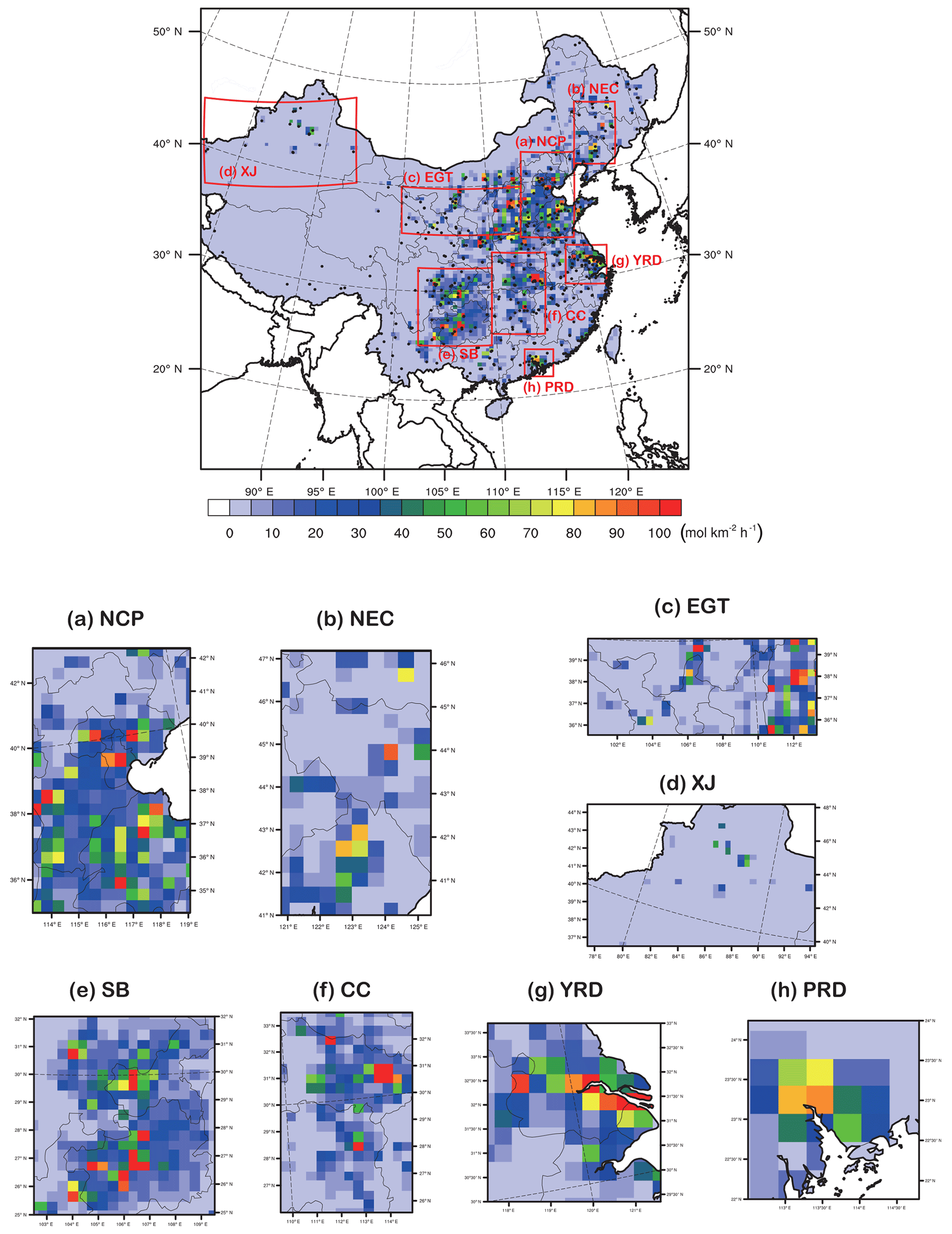
Figure 2Spatial distribution of the a priori SO₂ emissions used in this study. Regions defined in the red rectangles are (a) NCP (the North China Plain), (b) NEC (northeastern China), (c) EGT (the Energy Golden Triangle), (d) XJ (Xinjiang), (e) SB (the Sichuan Basin), (f) CC (central China), (g) YRD (the Yangtze River Delta), and (h) PRD (the Pearl River Delta). The color coding of the regional plots relates to the color bar of the national plot. (Units are in mol km⁻² h⁻¹.)

Download

Table 1WRF-Chem model configuration.

Download Print Version | Download XLSX

2.2 A priori emissions

The Multi-resolution Emission Inventory for China (MEIC) (Zhang et al., 2009; Lei et al., 2011; He, 2012; Li et al., 2014) for January 2010 is used as the a priori emission input. Unlike in other countries, the national emission inventories in China (e.g., NEI05-08-11-14-17) are provided in a timely manner and updated for the public. It has previously been stated that “there are no official data about how much air pollutants are emitted by China every year. The inventories developed by researchers often lag several years behind the present” (Zheng et al., 2018). MEIC is the only publicly available emission inventory dataset released by the Tsinghua University research community. In the MEIC, the total amount of sectoral emissions at the national and provincial levels has generally been estimated based on the bottom-up approach, which relied on available statistical information concerning activities (energy, industrial production, vehicles, and so on.), emission factors, and end-of-pipe control levels. Due to the large burden of work and the availability of statistical data, the MEIC emission inventory is not updated annually (e.g., the public versions are MEIC-2010-2012); thus, there are always a few years of time lag when applying the MEIC EI (emissions inventory) for research studies. In addition, to drive the regional air quality models, the annual/monthly total amounts of emissions at the national and provincial level are allocated spatially and temporally to generate an hourly gridded emission input for the model. Concerning temporal allocation, as many emission sources have large diurnal and weekly variability that is not fully represented, arbitrary hourly/weekly factors were used in preparing the hourly gridded emissions for the air quality models. Thus, both the uncertainties of the statistical information and the spatial–temporal allocation could cause inaccurate representation of the hourly gridded emission input and affect the performance of the model application.

The preprocessing method used to convert the original emission inventory (in 0.25×0.25^∘) to match the model grid spacing (40 km) is the same as that used in Chen et al. (2019). The spatial distribution of a priori SO₂ emissions in the simulation domain is shown in Fig. 2. A number of studies have revealed the uncertainties of the bottom-up emission inventories, including the energy statistics at the national and provincial levels (e.g., Hong et al., 2017) and emission factors from different industry sectors (e.g., Zhao et al., 2011, 2017). Our purpose is to investigate not only the uncertainty of the a priori MEIC emissions but also the capability of the DA system to dynamically update the SO₂ emissions using surface observations as constraints. For this purpose, the changes of SO₂ emissions from the a priori emission year (2010) to our focus years (2015 and 2016) are emphasized.

There are several different driving factors in different regions that may lead to inhomogeneous changing trends during the years examined (especially from 2010 to 2015). As the Chinese government has implemented desulfurization legislation (since 2005–2006 but with stricter control of the actual use of installations since 2008–2009) and strict control strategies to ensure the air quality during winter seasons since 2013, significant SO₂ emission reductions are expected to have occurred since 2010. However, there are converse results for certain regions. For example, Cheng et al. (2017) and Zhi et al. (2017) conducted a village energy survey for the rural areas in Hebei Province and revealed a huge amount of missing rural raw coal for winter heating. For Beijing and Baoding, rural emissions from raw coal in winter were higher than those from the industrial and urban household sectors in the two cities in 2013. Considering the living habits of residents in northern China, this may imply an extreme underestimation of rural household coal consumptions by the China Energy Statistical Yearbooks. Additionally, multi-satellite data (Ozone Monitoring Instrument – OMI, the SCanning Imaging Absorption spectroMeter for Atmospheric CartograpHY – SCIAMACHY) revealed increasing SO₂ emissions due to energy industry expansion in northwestern China (The central government of the People's Republic of China, 2012, 2014), especially new power plant installations in Xinjiang and Shaanxi, e.g., in Shen et al. (2016) and Koukouli et al. (2016). Eight different regions are illustrated to address this issue. Northern China is divided into two regions, the North China Plain (NCP) and northeastern China (NEC), as the North China Plain is more emission-intensive and may experience stricter control strategies than those in northeastern China during winter haze periods. Northwestern China is also divided into two regions, including the EGT (the Energy Golden Triangle) and XJ (Xinjiang). Southern China is divided into four regions according to its geographic characteristics, including the SB (Sichuan Basin), CC (central China), YRD (the Yangtze River Delta), and PRD (the Pearl River Delta). The spatial distributions of the SO₂ emissions in the eight regions are also illustrated in Fig. 2.

In terms of the temporal allocation, we applied predefined functions for the diurnal variations of the a priori SO₂ emissions, but the hourly factors are the same for all of the sectors and all of the grids, which is not optimal. Actually, different sectors/regions may have different hourly emission factors. For example, the transportation sector may produce peak emissions during rush hours, and the industry sector may produce emissions during the production period. Thus, it is not optimal to use the same hourly emission factors for all sectors. For regions in different time zones, different hourly emission factors are also expected. The diurnal variability is not publicly released and is highly uncertain, which introduces large uncertainty into the simulations. We also want to investigate whether the DA system can capture the diurnal variations of SO₂ emissions using the hourly surface SO₂ concentrations as constraints.

2.3 GSI 3D-Var DA system

Building upon the GSI 3D-Var DA system used in Chen et al. (2019), we extended the system capability of assimilating surface SO₂ observations. The algorithm and methodology for the aerosol DA are described in Chen et al. (2019). Here, only the differences implemented for the SO₂ DA are addressed.

The SO₂ observation operator is rather simple, and is written as $\prod m={\mathit{\rho }}_{\mathrm{c}}{M}_{{\mathrm{SO}}_{\mathrm{2}}}$. The unit of the model-simulated $M_{{\mathrm{SO}}_{\mathrm{2}}}$ is parts per million (ppm); thus, multiplication by the unit conversion ρ_c was required to convert the units to micro grams per cubic meter (µg m⁻³) for consistency with the observations. The observation errors are calculated similarly to the process in Chen et al. (2019). In the data quality control process, SO₂ observational values larger than 650 µg m⁻³ or observations leading to innovations/deviations (observations minus the model-simulated observations determined from the first-guess fields) exceeding 100 µg m⁻³ were not used. The BECs (background error covariance) values were computed using the “National Meteorological Center (NMC)” method (Parrish and Derber, 1992) by taking the differences of the 24 and 12 h WRF-Chem forecasts valid at the same time for 60 pairs of data valid at either 00:00 or 12:00 UTC over January 2015. The standard deviations over the whole domain are shown in Fig. S1 in the Supplement.

2.4 WRF-Chem/EnKF DA system

The WRF-Chem/EnKF assimilation system framework (Fig. 1) was used. Similar to other ensemble DA configurations in WRF-Chem, such as WRF-Chem/Dart (Mizzi et al., 2016), WRF-Chem is used to propagate the initial ensemble forward in time. The EnSRF is used to assimilate the observations and update the meteorological conditions, chemical initial conditions, and/or emissions. The differences relative to WRF-Chem/Dart are mainly in the assimilation engine (the ensemble adjustment Kalman filter is used in WRF-Chem/Dart, whereas the ensemble square root filter is used in our study), the structure of the state variables (meteorological and chemical initial/conditions are used in WRF-Chem/Dart, whereas chemical initial condition/emissions are used in our study), the cycling procedures, and so on. The WRF-Chem/EnKF assimilation system framework (Fig. 1) is very similar to that of Peng et al. (2017). Peng et al. (2017) focused on the joint analysis of both the initial conditions and emissions of PM_2.5 and addressed the forecasting skill improvement from using the EnKF system. Here, we focus on the estimation of SO₂ emissions, aiming to investigate the system capability of reflecting the spatial–temporal emission changes using observational data as constraints. In addition, instead of setting the emission scaling factors as control variables and adjusting the emissions by timing the scaling factors, we attempted to set emissions directly as control variables, which allowed for adjustments to be made by adding absolute emission values. Using this method, the detection of new emission sources would become more flexible. As in the previous approach, the emission scaling factors were extremely large when a new emission source (e.g., a new power plant) occurred in an originally “clean” model grid (a priori emissions close to zero), with the scaling factor being so large that it might be treated as “unrealistic” and be filtered out in the system. The direct analysis of emissions is expected to be more appropriate for this case.

The ensemble square root filter (EnSRF, Whitaker and Hamill, 2002) algorithm is very similar to that in Peng et al. (2017), except for some differences, such as the state variables (changed from aerosols to SO₂ concentrations and emissions) and the inflation factor. In addition, the forecast model for emissions is also different from that in Peng et al. (2017). More details on the differences from Peng et al. (2017) are described below.

2.5 Observations

Hourly surface SO₂ concentrations for January 2015 and 2016 were obtained from the China National Environmental Monitoring Center (CNEMC). There are approximately 1600+ sites in our modeling domain (black dots in Fig. 2). As the 1600+ monitoring sites fall into 531 model grids, observations within the same grid are averaged (by latitude and longitude) for the purpose of statistical analysis and verification. The observation sites mostly span northern, central, and eastern China and are relatively sparse in western China. To ensure data quality before use in the DA, SO₂ observational values larger than 650 µg m⁻³ were deemed unrealistic and were not assimilated in the GSI 3D-Var or the EnKF DA system.

2.6 Experimental design

To qualitatively evaluate the deficiencies of the a priori SO₂ emissions, generate updated emissions for 2015 and 2016, and evaluate the improvements from the DA approach, five sets of experiments were conducted. The corresponding comparisons and purposes are listed in Table 2. The simulated periods were January of 2015 and 2016. The meteorological initial condition (IC) and boundary condition (BC) were updated from GFS analysis data every 6 h (for NO_DA) or 1 h (for CONC_DA and EMIS_DA) to prevent the meteorology simulation drifting. The same WRF-Chem configurations (Table 1) were used in all the experiments.

Table 2Experiments conducted in this study and the three groups of comparisons.

Download Print Version | Download XLSX

In the NO_DA experiment, a new WRF-Chem forecast was initialized every 6 h starting at 00:00 UTC on 20 December of the previous year to spin up the chemistry fields and was run through until 23:00 UTC on 31 January. The chemistry fields were simply carried over from cycle to cycle. The 2010-MEIC a priori emissions were used, assuming the same emissions as in 2010. For CONC_DA, the hourly surface observations were assimilated by GSI 3D-Var, and the SO₂ concentrations were updated every hour starting from 00:00 UTC on 1 January. The background of the first time step is from the NO_DA simulation, and those of the later time steps are all from the 1 h WRF-Chem forecast using the updated chemical fields of the previous assimilation cycle as the ICs. As the concentrations from CONC_DA are very close to the observations, the concentration differences between CONC_DA and NO_DA possibly indicated a model deficiency in reproducing the reality, which was mainly from the emission changes from 2010 to 2015/2016. The assumption is that the GFS 6 h analysis data provide good meteorological IC/BC values and that the model accurately simulated the meteorological conditions; thus, the emissions were the major deficiency in the model.

The EMIS_DA experiment with continuous hourly cycling of the WRF-Chem/EnKF was performed for January of 2015 and 2016. The initialization and spin-up procedures of the 50-member ensemble were conducted starting from 00:00 UTC on 29 December of the previous year to 00:00 UTC on 1 January of the next year. Then, the EMIS_DA cycle started at 00:00 UTC on 1 January. Following the procedure in Fig. 1, the EMIS_DA experiment started with conducting EnSRF analysis and generated both the updated SO₂ concentration fields for the current time step and the updated analyzed SO₂ emissions for the previous time step. In this hourly cycling approach, 1 h WRF-Chem/EnKF cycling was conducted for January of 2015 and 2016, and hourly analyzed SO₂ emissions were then obtained. We compared the 2015 emissions from EMIS_DA to the 2010 a priori emissions, as the emission differences between the 2015 analyzed emissions and the 2010 a priori emissions not only reflected the changes from 2010 to 2015 but also included the deficiencies in the 2010 a priori emission. We also compared the updated emissions between 2015 and 2016, as the differences between the 2016 analyzed emissions and the 2015 analyzed emissions reflected the pure emission changes from 2015 to 2016, as the deficiencies of the 2010 a priori emissions were offset in the subtraction. The emission control policies are discussed to investigate whether the emission changes are reasonable.

To investigate the impact of using analyzed emissions from the EnKF DA system, two forecast experiments (NO_DA_forecast and EMIS_DA_forecast) were conducted for the same period. Twenty-four-hour forecasts were performed at 00:00 UTC of each day from 1 to 31 January for 2015 and 2016. The original a priori emissions and the updated analyzed emissions were used in the NO_DA_forecast and EMIS_DA_forecast experiments, respectively. The chemistry initial conditions for each forecast in the two forecast experiments were from the 1 h cycling GSI 3D-Var (COND_DA) experiment. The meteorological IC and BC were all from GFS analysis and forecast data. The concentration differences between the two sets of 24 h forecasts reflect the effects of the updated emissions.

3.1 Spatial distribution

Figure 3 shows the observed and modeled monthly average surface SO₂ concentrations for January in 2015 and 2016. The observations show great differences between northern and southern China, reflecting the dominant role of heating-related emissions in northern China during the winter season. The high values in northern China also show localized characteristics (no smooth transitions from the high-value region to the surroundings) that reveal the localization of SO₂ emissions and transport. The NO_ DA experiment significantly overestimates the surface SO₂ in the Sichuan Basin and central China but underestimates it at several locations in northern China and Xinjiang. After GSI 3D-Var hourly cycling of the DA, the CONC_DA experiment results are very close to observations because they corrected most of the biases in NO_DA except for the very high values at some of the “hot spots” in northern China. The fact that the improvements at those locations are not significant may be due to the data filtering process, in which SO₂ data with either observed values larger than 650 µg m⁻³ or innovations/deviations (observations minus the model-simulated values determined from the first-guess fields) exceeding 100 µg m⁻³ were rejected. The differences between CONC_DA and NO_DA more clearly revealed the inhomogeneous emission changes in different regions. For 2015, a great SO₂ decrease from NO_DA to CONC_DA in most of the eastern and southern regions was found, but increases were observed in northeastern China, the Energy Golden Triangle, and Xinjiang, indicating that the 2010 January a priori emissions should be adjusted accordingly (following decreasing/increasing trends, respectively) to reflect the 2015 January status. The negative discrepancies in the eastern and southern regions are even larger for 2016, indicating continuous emission decreases in these areas.

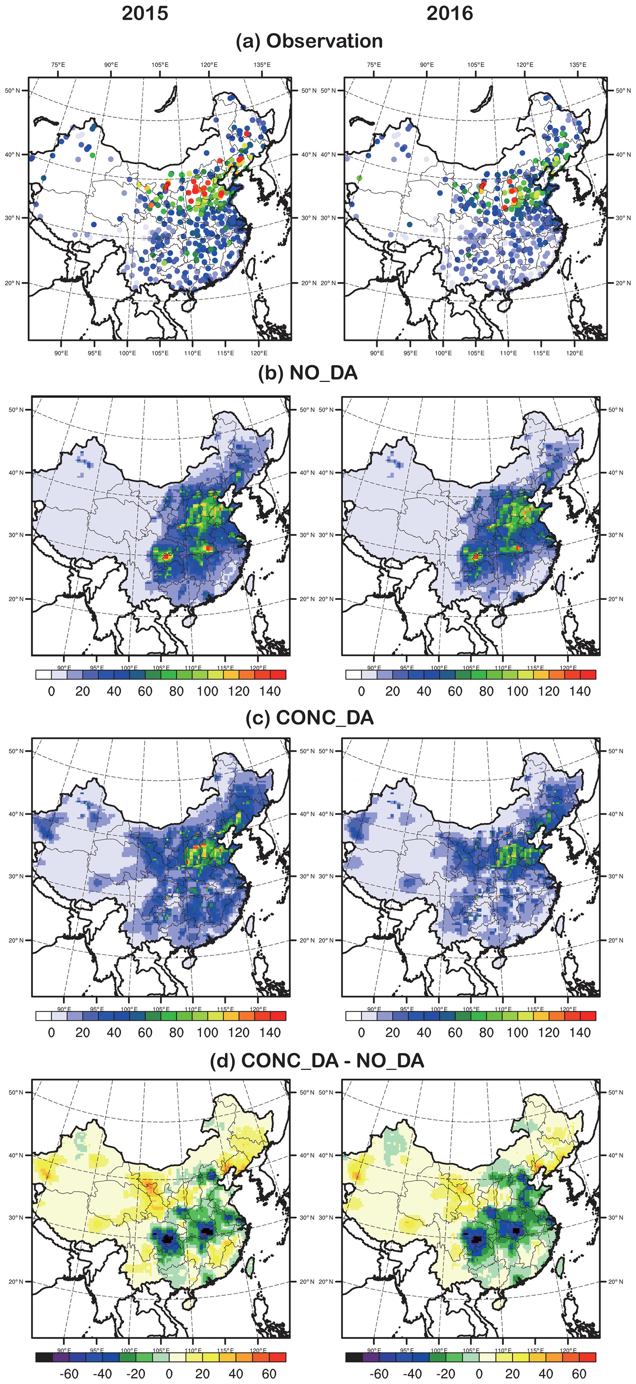
Figure 3Observed and modeled monthly average SO₂ concentrations for January in 2015 (left column) and 2016 (right column). (a) Observations, where the ranges of the different colors are the same as those of the color bars of (b) and (c); (b) NO_DA; (c) CONC_DA; and (d) CONC_DA − NO_DA. (Units: µg m⁻³.)

Download

To further investigate the deficiencies of the a priori emissions, the spatial distributions of the statistics (MEAN BIAS, RMSE, and CORR) at each observational site (which had more than two-thirds valid data in the month) in January of 2015 and 2016 for the two experiments are shown in Fig. 4. We start from the 2015 statistics and then address the differences relative to 2016. In NO_DA, consistent with Fig. 3, the surface SO₂ in southern China (the Sichuan Basin, central China, the Pearl River Delta, and the Yangtze River Delta) is generally overestimated by 20–50 µg m⁻³, but it is underestimated in northeastern China and the Energy Golden Triangle. The BIAS also showed localized characteristics with positive biases in megacities (e.g., Beijing), along with negative biases in the surroundings, indicating overestimated/underestimated emissions, respectively. There are also high RMSEs in northeastern China, the North China Plain, and the Energy Golden Triangle, indicating a wide spread of differences between observational data and NO_DA simulations, which may also indicate a model deficiency in reproducing strong temporal fluctuations (with the same daily emissions and fixed hourly factors as in the a priori emissions); the poor correlations (less than 0.5) at most of the sites also support this assumption. From year to year, the biases in 2016 are even more prominent. With GSI 3D-Var hourly cycling, the BIAS, RMSE, and CORR are greatly improved, as expected, while the improvements in northern China are smaller than those in southern China.

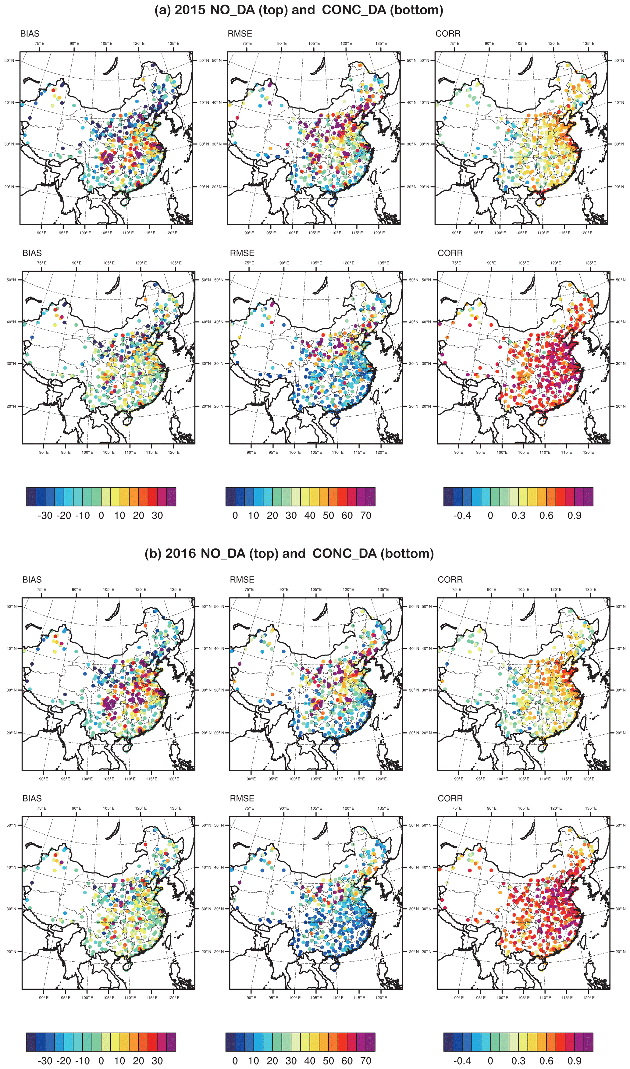
Figure 4The spatial distribution of the statistics between the model simulations and the observations for (a) January 2015 and (b) January 2016. The top row shows NO_DA vs. observations, whereas the bottom row shows CONC_DA vs. observations. (Units: µg m⁻³ for BIAS and RMSE.)

Download

3.2 Changes from 2015 to 2016

The differences between the January values of the 2 years (2015–2016) are shown in Fig. 5. Observations (Fig. 5a) mostly show decreases from 2015 to 2016 for most sites, especially in the North China Plain and southern China. In the NO_DA experiment (with the same emissions and different meteorology), some decreases are shown that reflect the meteorology condition differences between the 2 years, but the observed significant decreases in the North China Plain and southern China are not captured. CONC_DA (Fig. 5b) did reproduce the large decreases in the North China Plain and southern China from 2015 to 2016. From the difference between Fig. 5b and c, it can be assumed that factors other than meteorology (e.g., emissions control measures) play important roles in causing the decreases. CONC_DA failed to reproduce the large positive changes at three locations in the Energy Golden Triangle region, as CONC_DA failed to reproduce the high SO₂ concentrations in both years due to the data filtering processes.

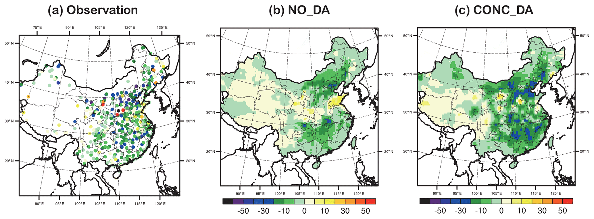
Figure 5Observed and modeled SO₂ ambient concentration changes (January 2016–January 2015). (a) Observations, where the ranges of different colors are the same as those in the color bars of (b) and (c); (b) NO_DA; and (c) CONC_DA. (Units: µg m⁻³.)

Download

4.1 Ensemble performance

In a well-calibrated system, when compared to the observations, the prior ensemble mean root mean square error (RMSE) would equal the prior “total spread”, defined as the square root of the sum of the observation error variance and the ensemble variance of the simulated observations (Houtekamer et al., 2005). The time series of the hourly prior ensemble mean RMSE and the total spread of surface SO₂ in the eight regions are shown in Fig. 6. The time series of the two months (January 2015 and January 2016) are given separately. Typically, the statistics at a single site for a certain period reflect the model biases and variances of errors at that site for the whole period. However, herein, the statistics for the eight regions were determined for all sites within the region at a 1 h frequency, which means that the statistics actually reflect the biases and error variances of the model simulations for those sites at every hour. As the emissions and meteorological conditions could be very different at sites in the same region, the RMSE for that region could be large. Due to the spatial–temporal inhomogeneity of emissions and meteorological conditions in different regions, the model shows different performances in terms of the differences in the RMSE. The “total spread” reflects the ensemble variances of the model-simulated values.

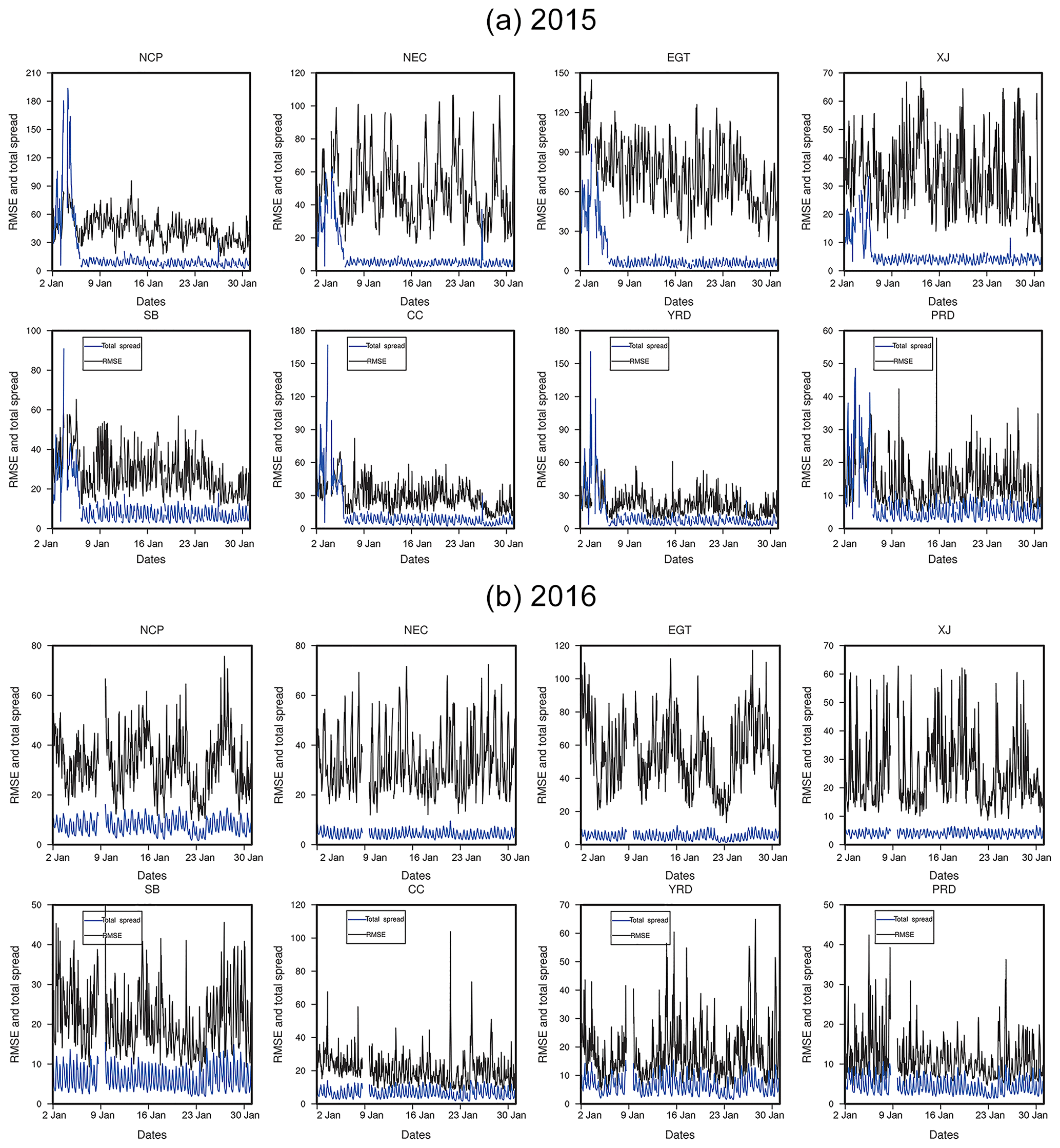
Figure 6Regional averaged RMSE and the total spread for (a) January 2015 and (b) January 2016 in eight regions. Time starts from 00:00 UTC. (Units: µg m⁻³.)

Download

The magnitudes of the total spread and the RMSE are influenced by the diurnal cycle and the pollution events (driven by meteorological patterns and emissions). As expected, all of the total spreads in the eight regions are smaller than the RMSE for almost the whole period, except those for the first few days in 2015. Because the lateral boundary and initial conditions of meteorology were also perturbed in addition to emission perturbation in the spin-up procedure, larger spreads were obtained in the first DA cycle, which may have remained for a short period. For all other periods without meteorological perturbations, insufficient spreads of SO₂ ensemble forecasts were shown, with the effects in the northern and western regions (North China Plain, northeastern China, the Energy Golden Triangle, and Xinjiang) being worse than those in southern regions (the Sichuan Basin, central China, the Yangtze River Delta, and the Pearl River Delta), as the prior ensemble mean RMSE values in the northern regions were much larger, but the total spreads were fairly constant. For the northern regions, the total spread (Fig. 6) was relatively small compared to the RMSE. This might indicate that the analyzed emissions converged gradually and that the background emissions (calculated according to Eq. 4) of different members in the DA cycling were similar, thus leading to the small spread. As the spread is small, some observations might be rejected in the DA outlier check, which may impact the DA performance. The distinction of the comparisons among different regions (the North China Plain vs. the Yangtze River Delta/Pearl River Delta) indicated the deficiencies of the perturbation procedure in the DA system when applied to northern regions. Further investigations should be conducted to generate larger spreads for northern regions in future studies.

4.2 Analyzed 2015 and 2016 emissions

The optimized SO₂ emissions obtained from the assimilations for January 2015 and 2016 are shown in Fig. 7. To address the changes from 2010 to 2015 and those from 2015 to 2016, the differences and ratios between the two groups (2010 vs. 2015 and 2015 vs. 2016) are given. For the comparison of 2015 analyzed emissions with 2010 a priori emissions, as real observations were used to constrain the 2015 emissions, the differences between the two sets of emissions actually reflect the adjustments based on the 2010 a priori emissions, which are needed to better capture observations; thus, the comparison not only reflects the changing trends from 2010 to 2015 but may also indicate the deficiencies of the 2010 a priori emissions. It should be noted that the two aspects are mixed when interpreting the results. While the comparison of 2015 analyzed emissions with 2016 analyzed emissions is more straightforward, as they are both produced using observation constraints, the differences between the two reflect the annual changes between the 2 years, and the impacts from a priori emission deficiencies are removed in the subtraction.

Figure 7Analyzed emissions for (a) January 2015 and (b) January 2016. (c) The differences of the 2015–2010 a priori inventory and (d) ratios of the 2015∕2010 a priori inventory. (e) The differences of 2016 − 2015 and (f) ratios of 2016∕2015. (Units are mol km⁻² h⁻¹ for (a), (b), (c), and (e)).

Download

Compared to the 2010 a priori emissions, the analyzed emissions for 2015 show different spatial changes (northern, western, and southern China). Large emission decreases in southern China (the Sichuan Basin, central China, the Yangtze River Delta, and the Pearl River Delta) are shown, but there are also some small emission increases in scattered regions. These increases are relatively small in absolute value (shown using light yellow in Fig. 7c), but the 2015∕2010 ratios can reach large numbers (shown using orange to red in Fig. 7d), as the a priori emissions in those regions are very small (Fig. 2); thus, minor changes lead to large ratios. For northern China (North China Plain and northeastern China), the change pattern is somewhat opposite. Emission increases are shown for most of the regions, with decreases only occurring at scattered points. Large 2015∕2010 increasing ratios are also shown in western China (Xinjiang and The Energy Golden Triangle), while the a priori emissions are very sparse in those two region; thus, the emission increases are more significant, which may indicate new emission sources. For the changes from 2015 to 2016, the pattern is rather homogenous across the whole domain, with decreases in almost all regions.

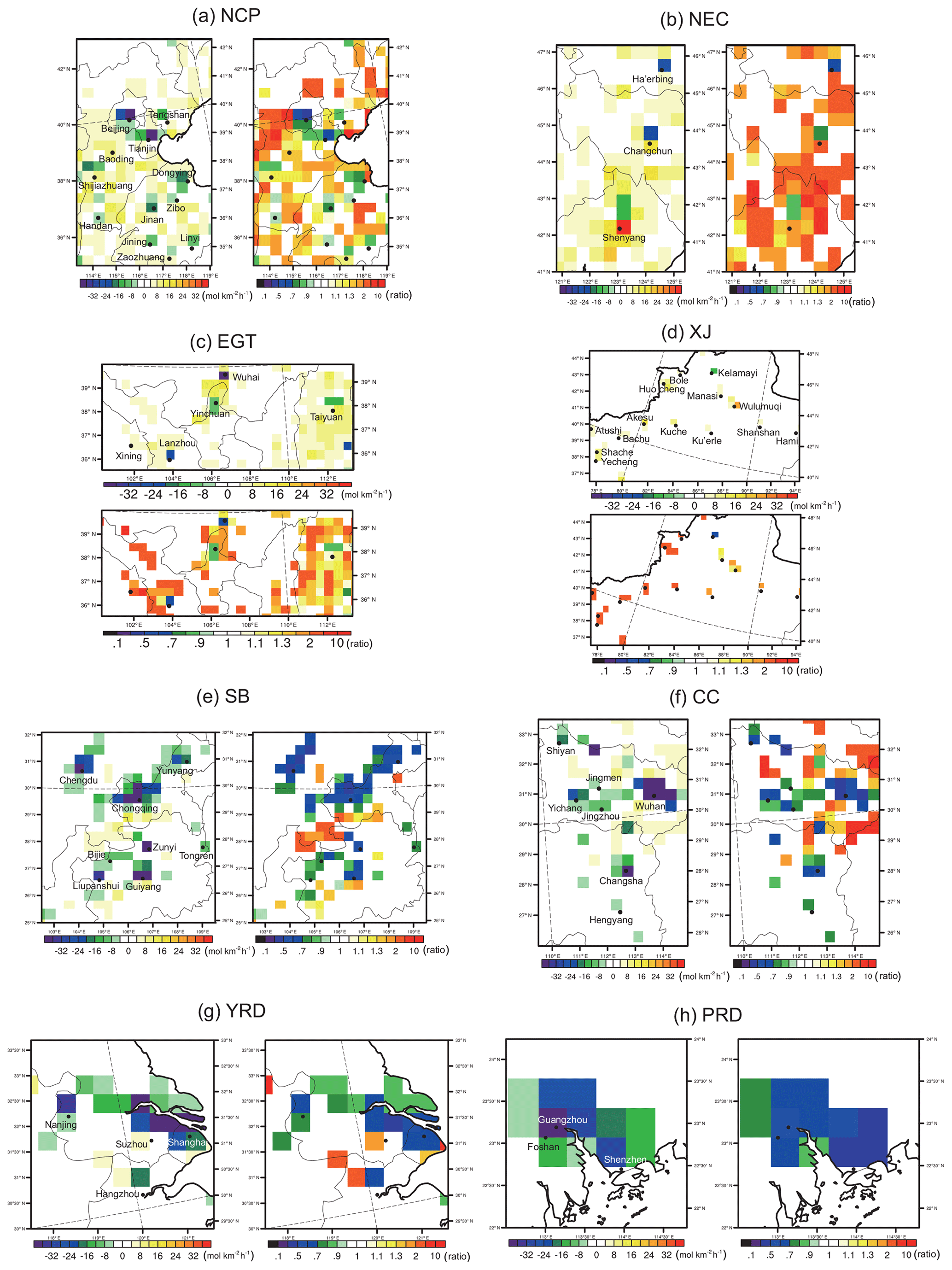
Figure 8The differences between the analyzed 2015 January emissions and the 2010 a priori emissions in eight regions. Left/top panels are emission differences of 2015 − 2010 (units: mol km⁻² h⁻¹), and right/bottom panels are the ratios of 2015∕2010 in each region.

Download

4.3 Changes in different regions

To further illustrate the changes in different regions, the details of eight regions are given in Fig. 8 (2015 vs. 2010) and Fig. 9 (2016 vs. 2015). Similar to Fig. 7, the emission changes in terms of absolute values (left panels) and ratios (right panels) are given for each region. To better understand the geographic changes, the center locations of some large cities (capital cities of provinces and municipal centers at the city level) in those regions are labeled. According to Fig. 7, the change patterns are different in northern, western, and southern China for 2015; thus, discussions are given based on this classification. We start from the comparison of the 2015 analyzed emissions with the 2010 a priori emissions, as there is a 5-year time lag between the two sets of emissions, along with large uncertainties; therefore, large changes are expected.

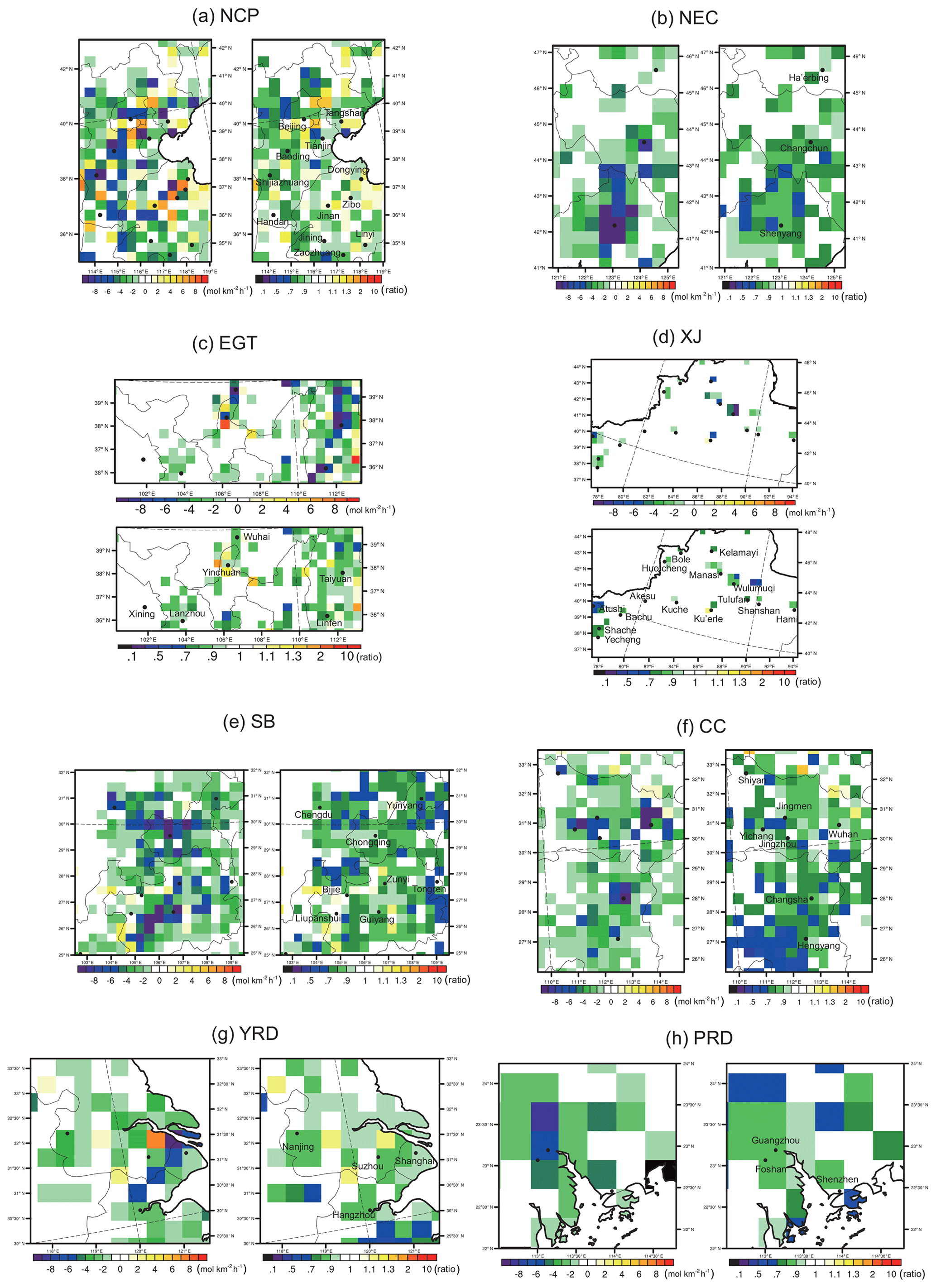
Figure 9Same as Fig. 8, but for the differences between the analyzed 2016 January emissions and the 2015 January emissions in eight regions. Left/top panels are emission differences of 2016 − 2015 (units: mol km⁻² h⁻¹), and right/bottom panels are the ratios of 2016∕2015 in each region.

Download

It is interesting to see that for northern China (North China Plain and northeastern China), the most significant decreases occur in or around large cities (city center locations are labeled as black dots). The phenomenon is very prominent in the North China Plain, as we can see some “cold” spots (grids with cold colors) in Fig. 8a, which are either overlapped by city center locations (Beijing, Tianjin, Xingtai, and Handan in the Beijing–Tianjin–Hebei region, and Dongying, Jinan, Zibo, and Jining in Shandong Province) or adjacent to the center locations (Shijiazhuang, Linyi, Zaozhuang). As the center locations are represented as latitudes and longitudes that do not cover entire city areas, there might be some shifting produced from interpreting the results when the city areas are too large (e.g., Shijiazhuang, Changchun, and Shenyang) and have been split into two or more grids in the model. While the results still indicate that the emissions in these larger cities decreased due to the strict control strategies from 2010 to 2015 (factory migration from urban regions to remote regions, desulfurized equipment in factories/vehicles, low-sulfur energy, etc.), there are some emission increases in the suburban and rural regions surrounding these larger cities, either due to emission migration from urban regions or new emission sources added due to urbanization development. The results might also indicate that the control strategies were executed at different levels in urban (more strict) and suburban–rural regions during the period from 2010 to 2015. In northeastern China, significant “cold spots” also occur in the three larger cities, including Ha'erbing, Changchun, and Shenyang, but increases mostly occur in other areas, indicating a similar trend to that in the North China Plain, in which large emission decreases occurred in bigger cities and mild emission increases occurred in suburban–rural regions from 2010 to 2015. In addition to the possible aforementioned reasons accounting for the different changes of urban and suburban–rural regions from 2010 to 2015, it should be noted that the month of January is during the heating season for the North China Plain and northeastern China, and the large areas of emission increase might also indicate some heating emissions (from energy that has not been statistically well recorded, e.g., crop combustion and residential coal combustion) that are missing from the a priori emissions.

In western China, where the emission intensities are not as high and the emission sources are relatively sparse, the changing emission trends from 2010 to 2015 are more obvious and are more meaningful for distinguishing new emission sources/regions. As some studies have revealed increasing SO₂ emissions due to energy industry expansion and relocation in northwestern China from OMI measurements (Ling et al., 2017), our 2015 analyzed emissions also show large emission increases in the whole area of the Energy Golden Triangle and Xinjiang, except for in very few larger cities (Yinchuan, Wuhai, Lanzhou, and Karamay, which is also known as Kelamayi). The emissions in other areas of the Energy Golden Triangle and Xinjiang almost all show increases from 2010 to 2015. Especially for Xinjiang, the increases in emissions are all attributed to the rapidly developing cities/counties, including Urumqi, Aksu (A'kesu), Korla (Ku'erle), Yecheng, Manas (Manasi), Tacheng, Huocheng, Bachu, Atushi, Shanshan and Shacheng. Koukouli et al. (2016) and Ling et al. (2017) used multi-satellite data to investigate the SO₂ load changes from 2004–2014 and 2005–2015, respectively, and identified locations with increases (including U'rumqi in Xinjiang and cities in northwestern China). They reported that “These belong to provinces with emerging economies which are in haste to install power plants and are possibly viewed leniently by the authorities, in favor of growth.” Our findings are also consistent with those of these two studies.

In southern China, decreasing changes are shown for large areas, especially in the Yangtze River Delta and the Pearl River Delta, in which decreasing trends in larger cities are clearly shown, e.g., in Shanghai, Nanjing, and Hangzhou in the Yangtze River Delta and in Guangzhou, Shenzhen, and Foshan in the Pearl River Delta, with relatively larger decreasing ratios in more well-developed cities. In the Sichuan Basin and central China, the decreases in larger cities are also significant, and different extents are achieved in cities of different levels. For Chengdu, Chongqing, Zunyi, Guiyang, and Yunyang in the Sichuan Basin and Wuhan and Changsha in Central China, approximately 40 %–50 % reductions are shown from 2010 to 2015. For other larger cities (municipal centers of cities), 20 %–30 % reductions are shown.

As previously mentioned, the comparisons between the 2015 and 2016 analyzed emissions (Fig. 9) are more straightforward and reflect the necessary emission changes from 2015 to 2016, as the uncertainties in the a priori emissions are subtracted. As expected, decreasing trends are shown for almost all of the labeled cities, indicating the continuing strict execution of control strategies. However, there are still some grids with emission increases (approximately 10 %–30 %) in surrounding regions, especially in the North China Plain, which might reflect the emission increase from January 2015 to January 2016. As shown in Fig. 10 of Chen et al. (2019), the temperature in January 2016 was much colder than that in 2015, and the emission increases at those points may indicate heating-related emissions. Compared with Fig. 8 (2015 vs. 2010), the changes from 2015 to 2016 (both increases and decreases) are much milder in Fig. 9.

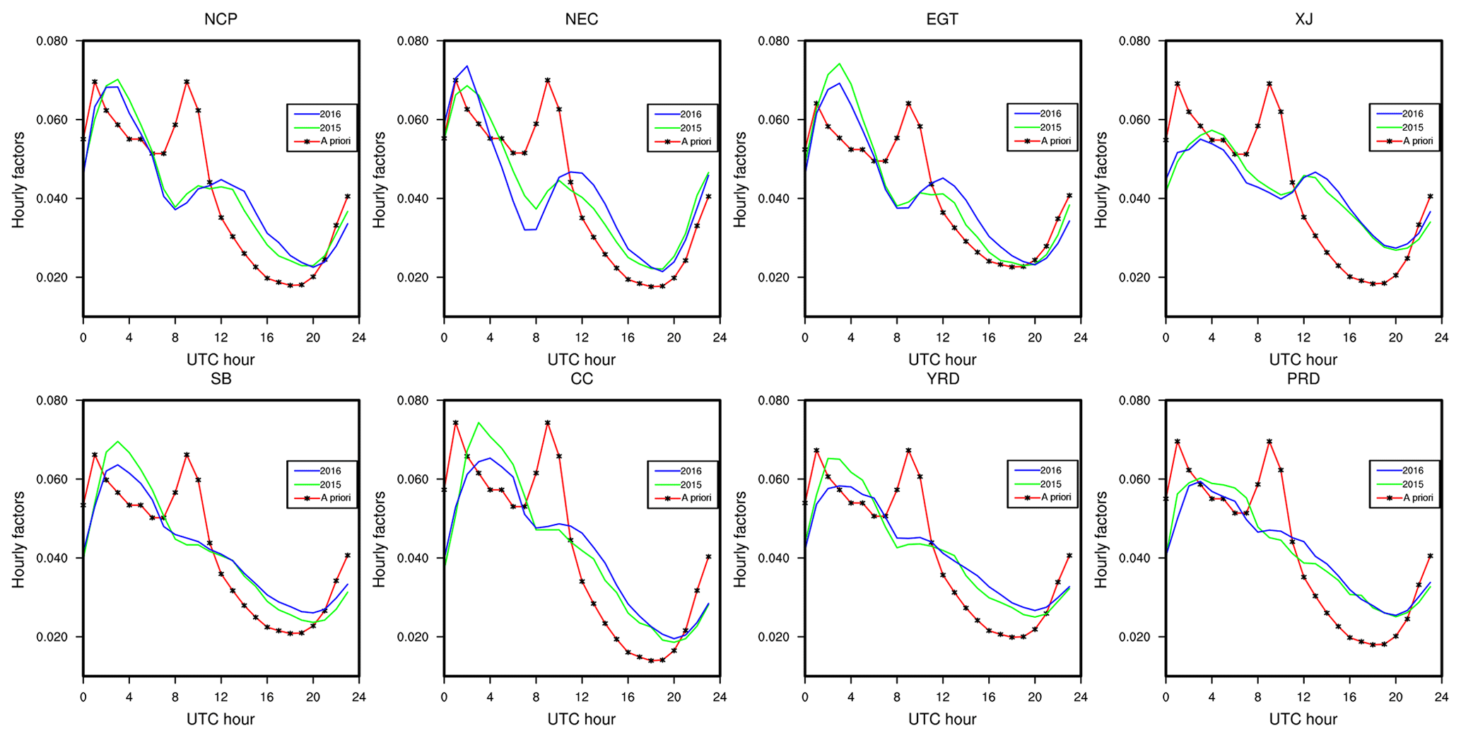
Figure 10Hourly factors in the a priori emission inventory and those derived from the EMIS_DA experiment in eight regions.

Download

The regional averages of the 2015 and 2016 January emissions are summarized in Table 3. In northern China (North China Plain and northeastern China) and western China (the Energy Golden Triangle and Xinjiang), the 2015 analyzed emissions are all larger than the 2010 prior emissions. The increase percentages are 12.7 %, 49.4 %, 25.6 %, and 72 % for the North China Plain, northeastern China, the Energy Golden Triangle, and Xinjiang, respectively, indicating an increasing trend from 2010 January to 2015 January, either due to emission increases in reality (possibly in the Energy Golden Triangle and Xinjiang) or uncertainties in the 2010 a priori emissions (possibly in the North China Plain and northeastern China). The largest increase occurred in Xinjiang, reaching 72 %, which is consistent with the previous findings of newly added emission sources in that region. In southern China, the 2015 analyzed emissions are all smaller, and the decreasing ratios are −10.5 %, −9.9 %, −13.8 %, and −22.9 % for the Sichuan Basin, central China, the Yangtze River Delta, and the Pearl River Delta, respectively. For the changes from 2015 to 2016, decreasing trends are shown for all regions, with the ratios ranging from −5.3 % to −16.1 %.

Table 3A priori and analyzed January emissions and the changing ratios for 8 regions (units: 10⁶ kg d⁻¹).

Download Print Version | Download XLSX

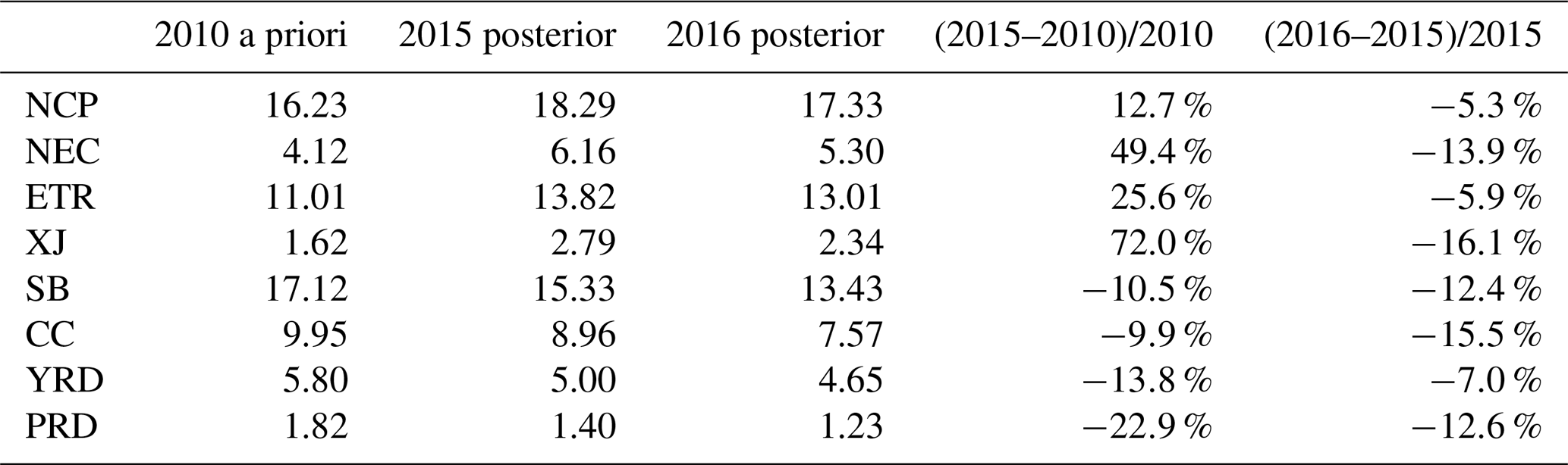
In the recent study by Zheng et al. (2018), the 2010–2017 trends of anthropogenic emissions in China were investigated. According to the bottom-up approach, the annual total amounts of SO₂ emissions were calculated to be 27.8, 16.9, and 13.4 Tg for the years 2010, 2015, and 2016, respectively. The 2010 to 2015/2016 decreases were mostly attributed to the power and industry sectors due to the strict pollution control measures implemented for these two sectors. The sectoral distribution of emissions have changed significantly over recent years, and emissions other than those from power and industry have occupied larger portions, especially for the residential sector, as the current control policies have limited effects on reducing emissions from the residential sector. According to Zheng et al. (2018), the national total SO₂ emissions decreased by 20.8 % from 2015 to 2016. Our derived changes ratios for the month of January in most of the regions (NEC, XJ, SB, CC, and the PRD) are comparable (13.9 %, 16.1 %, 12.4 %, 15.5 %, and 12.6 %, respectively, see Table 3), but the change ratios for NCP, ETR, and YRD are (relatively) smaller. As discussed in Zheng et al. (2018), bottom-up emission estimates are uncertain due to incomplete knowledge of the underlying data, and uncertainties are larger when emissions are contributed by scattered emission sources. Especially for the residential sector, the effectiveness of the measures (e.g., phasing out of small high-emission stoves and the banning of coal heating) is difficult to validate due to the lack of inspections; thus, higher uncertainties may arise for regions in which residential emissions are relatively important.

4.4 Hourly factors

As hourly observations were used to constrain the emissions, analyzed emissions at an hourly frequency were obtained, which provided us an opportunity to investigate the hourly emission factors from observations. To retrieve the hourly factors, the emissions during each hour (24 h) are averaged based on the EMIS_DA experiment for the whole period (2–31 January ). The retrieved hourly factors for 2015 and 2016 and the 2010 a priori emissions are shown in Fig. 10. The a priori hourly factors are given arbitrarily, with two peaks during the day at 01:00 UTC (09:00 BJ time – Beijing time) and 09:00 UTC (17:00 BJ time) to reflect the emissions during rush hours. The retrieved hourly factors in northern and western China showed two peaks at approximately 02:00 UTC (10:00 BJ time) and 12:00 UTC (20:00 BJ time), but the second peak is obscure in southern regions. In addition, the second peak of the hourly factors in the northern and western regions is much lower than the first, which was different from the predefined curve. In Xinjiang, the peaks occurred later than in the other regions, indicating that the time zone differences caused a different energy consumption/emission pattern. It should be noted that the hourly factors were derived from the analyzed emissions constrained from ambient concentration observations; thus, the response times from emissions to ambient concentrations were simplified in the assimilation system. Although the background emissions contain the information from the previous cycles, and may, therefore, help to pass the response information, there might still be some time lag in the retrieved hourly factors, which should be further verified.

5.1 Changes of spatial statistics

Figures 11 and 12 show the performances of the NO_DA_forecast and EMIS_DA_forecast experiments for January 2015 and 2016, respectively. Statistics, including the BIAS (bias, equal to the difference between the modeled value and the observational value, representing the overall model tendency), RMSE (the root mean square error/root mean square deviation, equal to the square root of the second moment of the differences between the model values and the observational values, reflecting both model biases and error variances), and CORR (the correlation coefficient, equal to the linear relationship between the modeled values and the observational values), were chosen to evaluate the two forecast experiments with a priori emissions and analyzed emissions, respectively. For a single site, the three statistics (BIAS, RMSE, and CORR) may change in two directions – for example, the BIAS (the bias of the absolute emission amount) may get worse, but the RMSE (error variance) and CORR (in terms of the diurnal or day-to-day emission changes) may get better. To fairly evaluate and show the overall changes, the 531 lumped sites were classified into five different groups to reflect the differences in the statistics. The classification and performance are listed in Table 4. The spatial distributions of the NO_DA_forecast statistics for each site are given in Figs. 11a and 12a. To better illustrate the changes of the statistics after applying the analyzed emissions, the differences (EMIS_DA_forecast − NO_DA_forecast), instead of the absolute values, are shown for the five defined groups in Figs. 11b–f and 12b–f. Specifically, the absolute values of the BIAS were used in the difference calculation.

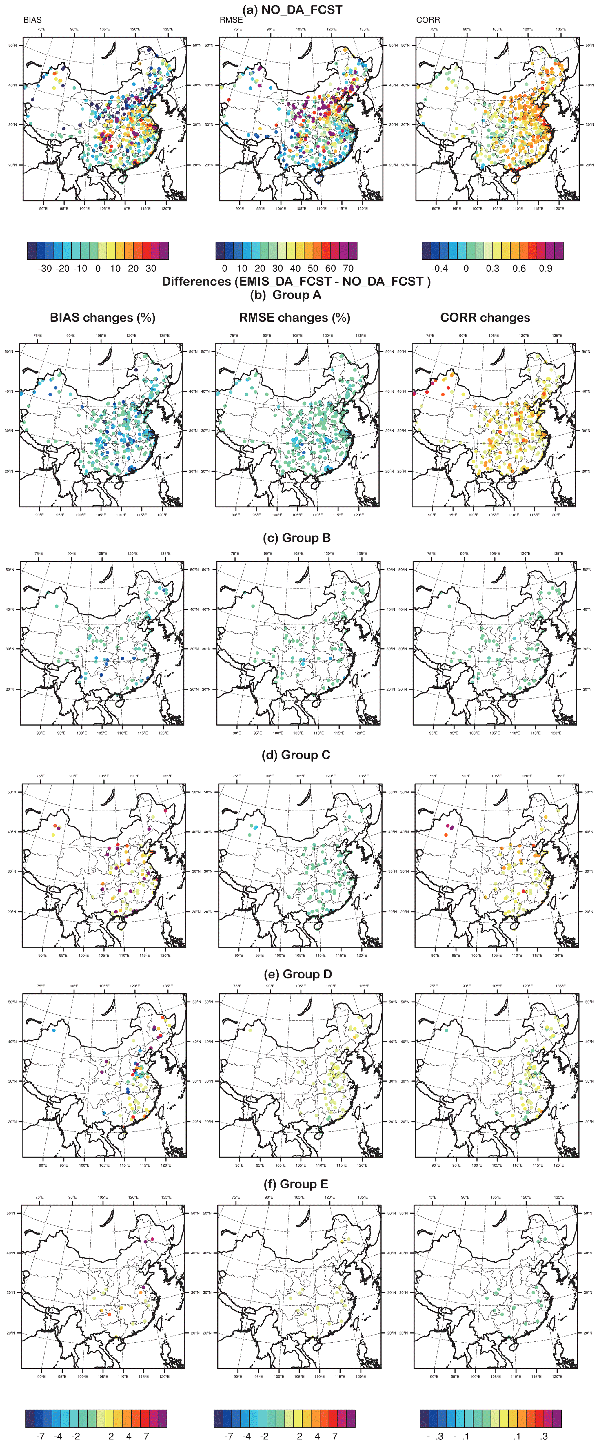
Figure 11The spatial distribution of the error statistics between the model simulations and the observations for January 2015. (a) Statistics between NO_DA_FCST and the observations, with BIAS and RMSE in micrograms per cubic meter; (b–f) the statistics improvements from NO_DA_FCST to EMIS_DA_FCST for different groups of sites (classification in Table 4), with the BIAS and RMSE improvements shown as percentages. The color bars are the same for (b)–(f) and are only shown in (c) and (f) to save space.

Download

Figure 12Same as Fig. 11, but for January 2016.

Download

Table 4Overall statistical changes of the EMIS_DA_FCST experiment compared with the NO_DA_FCST experiment.

Download Print Version | Download XLSX

Concerning single statistics, the BIAS, RMSE, and CORR are improved at 383, 444, and 426 sites, respectively, for the year 2015 (Table 4), while there are 524 total valid sites over the whole domain. That is to say that the ratios of sites improved are 73 %, 85 %, and 81 %, respectively, as determined using BIAS, RMSE, and CORR as the single criterion. When considering the overall performance using the three statistics, 300 sites (57 %) are fully improved (BIAS/RMSE decrease and CORR increase), 138 sites (26 %) are partially improved (either the BIAS and RMSE improved or the RMSE and CORR improved), only 16 sites (3 %) show an overall deterioration of performance, and the remaining approximately 13 % of sites could not be justified. The performance in 2016 is even better than that in 2015, with the fully improved (overall worse sites) being more (less) compared with the 2015 case.

Figure 11b shows that overall improvements are achieved over the whole domain, with the largest BIAS corrections occurring at sites in the Sichuan Basin, central China, the Yangtze River Delta, and the Pearl River Delta (reaching 60 %–70 % reductions) and the largest CORR improvement occurring in Xinjiang (reaching 0.35). The sites that are partially improved (Fig. 11c, d) and unclassified (Fig. 11e) are not in specific regions but are scattered through the whole domain. The sites that showed an overall deterioration of performance (Fig. 11f) are very few, and the variances are relatively small. Consistent with Table 4, the performance in 2016 (Fig. 12) is even better than that in 2015 (Fig. 11), with the BIAS corrections being more significant, especially in the Sichuan Basin, central China, the Yangtze River Delta, and the Pearl River Delta, and the CORR improvements are even larger in Xinjiang.

5.2 Time series of the regional mean

Figure 13 shows the time series of the regional mean forecasts (NO_DA_forecast and EMIS_DA_forecast) and the observed SO₂ concentrations in eight regions for 2015 and 2016. From the aspect of the regional mean, forecasts with a priori emissions are severely overestimated in southern China (the Sichuan Basin, central China, the Yangtze River Delta, and the Pearl River Delta), and the overestimations are largely corrected in the forecasts with analyzed emissions. For northeastern China, the Energy Golden Triangle, and Xinjiang, forecasts with a priori emissions are underestimated, and forecasts with analyzed emissions helped to correct the biases. It is surprising to see that the regional averages in the North China Plain match well with the observations, although the site-to-site comparisons (Figs. 11, 12) show large biases at single sites. As the sites in one region are averaged, the positive/negative biases among different sites might be offset in the averaged time series. For this reason, the RMSE and CORR of all the hourly data in one region are also calculated for verification.

Figure 13Time series of the regional mean SO₂ concentrations from the observations and from model simulations with the a priori and analyzed (posterior) emissions for (a) January 2015 and (b) January 2016 in eight regions. Time starts from 00:00 UTC. (Units: µg m⁻³.)

Download

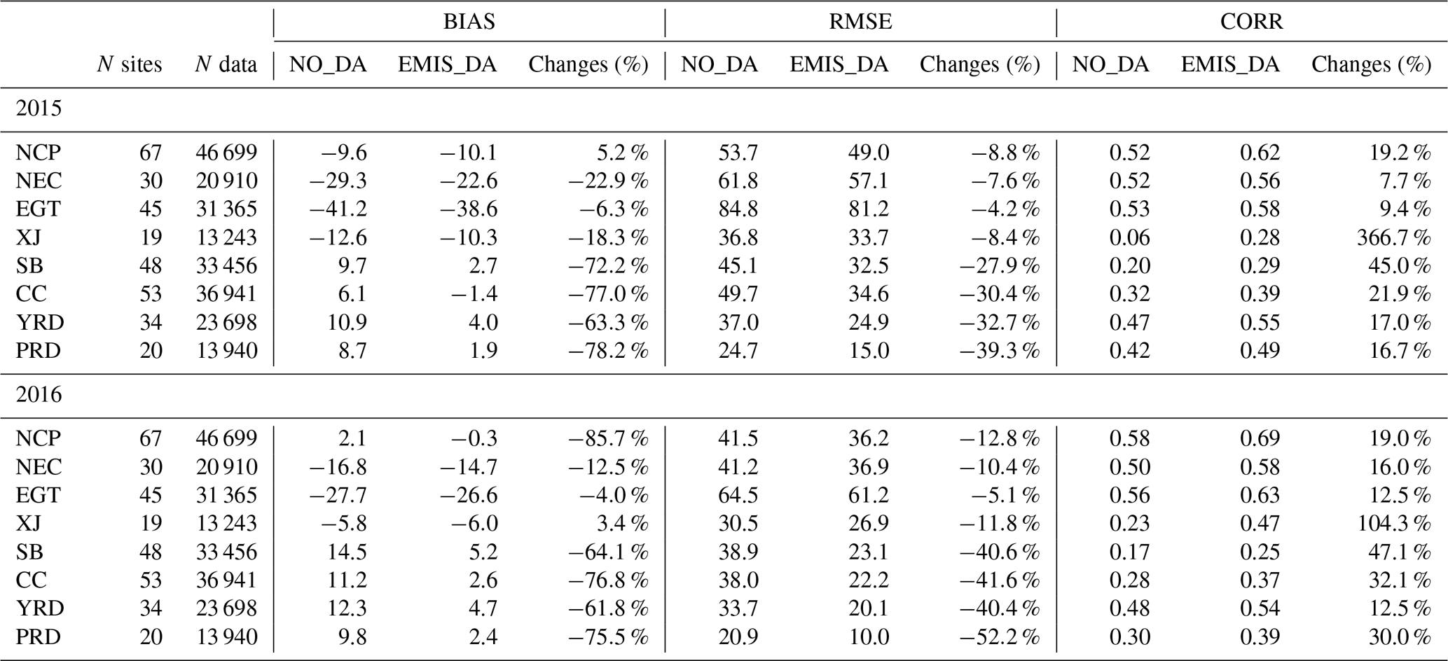
The statistics of the BIAS, RMSE, and CORR in the eight regions are given in Table 5. From the aspect of the regional mean, the improvements obtained after applying the analyzed emissions are more significant in southern China than in northern China, with the RMSE decreased by 27.9 %–39.3 %, the BIAS decreased by 63.3 %–78.2 %, and the CORR increased by 16.7 %–45.0 % for the year 2015. For northern China, although the improvements are not as large, the BIAS still decreased (except in the North China Plain), and the decreasing ratio ranged from 6.3 % to 22.9 %, while the RMSE decreased by 4.2 %–8.8 % and the CORR increased by 7.7 % to 366.7 %. The largest CORR increase occurred in Xinjiang, changing from 0.06 to 0.28, indicating that the newly added emission sources in the analyzed emissions are necessary. Compared with 2015, the improvements in 2016 are also larger, which is consistent with previous discussions.

Table 5Statistics of the EMIS_DA_FCST and NO_DA_FCST experiments in eight regions (units: µg m⁻³ for BIAS and RMSE).

Download Print Version | Download XLSX