the Creative Commons Attribution 4.0 License.
the Creative Commons Attribution 4.0 License.
 | 26 Jun 2019
IAP-AACM v1.0: a global to regional evaluation of the atmospheric chemistry model in CAS-ESM
Ying Wei
Xueshun Chen
Huansheng Chen
Jie Li
Zifa Wang
Wenyi Yang
Baozhu Ge
Huiyun Du
Jianqi Hao
Wei Wang
Jianjun Li
Huili Huang
In this study, a full description and comprehensive evaluation of a global–regional nested model, the Aerosol and Atmospheric Chemistry Model of the Institute of Atmospheric Physics (IAP-AACM), is presented for the first time. Not only are the global budgets and distribution explored, but comparisons of the nested simulation over China against multiple datasets are investigated, which benefit from access to Chinese air quality monitoring data from 2013 to the present and the “Model Inter-Comparison Study for Asia” project. The model results and analysis can help reduce uncertainties and aid with understanding model diversity with respect to assessing global and regional aerosol effects on climate and human health, especially over East Asia and areas affected by East Asia. For the global simulation, the 1-year simulation for 2014 shows that the IAP-AACM is within the range of other models. Overall, it reasonably reproduced spatial distributions and seasonal variations of trace gases and aerosols in both surface concentrations and column burdens (mostly within a factor of 2). The model captured spatial variation for carbon monoxide well with a slight underestimation over ocean, which implicates the uncertainty of the ocean source. The simulation also matched the seasonal cycle of ozone well except for the continents in the Northern Hemisphere, which was partly due to the lack of stratospheric–tropospheric exchange. For aerosols, the simulation of fine-mode particulate matter (PM2.5) matched observations well. The simulation of primary aerosols (normalized mean biases, NMBs, are within ±0.64) is better than that of secondary aerosols (NMB values are greater than 1.0 in some regions). For the nested regional simulation, the IAP-AACM shows the superiority of higher-resolution simulation using the nested domain over East Asia. The model reproduced variation of sulfur dioxide (SO2), nitrogen dioxide (NO2), and PM2.5 accurately in typical cities, with correlation coefficients (R) above 0.5 and NMBs within ±0.5. Compared with the global simulation, the nested simulation exhibits an improved ability to capture the high temporal and spatial variability over China. In particular, the R values for SO2, NO2 and PM2.5 are increased by ∼0.15, ∼0.2, and ∼0.25 respectively in the nested grid. Based on the evaluation and analysis, future model improvements are suggested.
- Article
(14245 KB) -
Supplement
(955 KB) - BibTeX
- EndNote


Atmospheric composition can affect climate and environment via direct and indirect effects (Houghton et al., 2001). The composition of the troposphere has changed a lot due to anthropogenic activities over the past decades (Akimoto, 2003; Tsigaridis et al., 2006). Changes in the concentration of trace gases such as sulfur dioxide (SO2) and nitrogen oxides () have a substantial impact on acid deposition (Mathur and Dennis, 2003), atmospheric oxidation (Calvert, 1984), and gas–particle transformation processes (Saxena and Seigneur, 1987). Aerosols formatted from these precursor gases, in addition to aerosols from other sources, have a direct radiative forcing. By modifying cloud properties, the aerosols also have important indirect effects. As reported in the Fifth Assessment Report (AR5) of the IPCC (Myhre et al., 2013), the radiative forcing of aerosols ranges from −1.9 to −0.1 W m−2, with the direct radiative forcing ranging from −0.85 to 0.15 W m−2. With better model performance and a more robust observation network, AR5 achieved increasing confidence in the assessment compared with AR4 (Boucher et al., 2013); however, radiative forcing associated with aerosols still has large uncertainties. In addition, aerosols have adverse impacts on human health, including respiratory diseases, cardiovascular risk, and lung cancer, which has drawn increasing public attention (Burnett et al., 2014; Pope et al., 2011; Powell et al., 2015). It is necessary to represent the key physical and chemical parameters controlling trace gases and aerosols in order to quantify these adverse effects and project the influence of aerosols in the future.
Chemical transport models (CTMs) are mathematical tools for studying the evolution of chemical constituents in the atmosphere. CTMs have irreplaceable advantages in terms of source and sink assessment of trace gases, historical process reproduction, and future scenario projection. In addition to observations and laboratory simulations, CTMs have become the main method for atmospheric environmental research (Wang et al., 2008). However, there are numerous uncertainties affecting model results (e.g. meteorology, emissions and model framework, and physiochemical schemes). Therefore, model evaluation is essential for model development and scientific analysis. To date, many assessments with a single model using various observation datasets and multi-model inter-comparisons (with or without observations) have provided us with a comprehensive understanding of model performance and uncertainty. For example, Badia et al. (2017) evaluated the gas-phase chemistry of the Multi-scale Online Nonhydrostatic Atmosphere Chemistry model (NMMB-MONARCH), Mann et al. (2010) evaluated both mass concentration and number concentration of the Global Model of Aerosol Processes (GLOMAP), and Tsigaridis et al. (2014) gave a detailed evaluation of organic aerosol in the Aerosol Comparisons between Observations and Models Project (AeroCom). However, evaluations against site observations have mainly focused on America and Europe and are inadequate for East Asia (EA) due to data limitations (Søvde et al., 2012; Lee et al., 2015; Kaiser et al., 2019). The spatial distribution of aerosols affects the estimation of radiative forcing (Shindell et al., 2013; Giorgi et al., 2003). Thus, using more observations to assess the model results helps to reduce the uncertainties of the climate effect prediction over EA.
Along with economic development and urbanization, most megacities in China have been plagued by haze in recent years. Therefore, there have been many observation and simulation studies addressing particulate matter. The model studies have mainly focused on the relationship between haze and weather conditions (Zhang et al., 2015; Tie et al., 2015, 2017), pollutants source apportionment (L. T. Wang et al., 2014; Y. Wang et al., 2014), and the chemical mechanism of particulate formation (Cheng et al., 2016). Regional models are more often used in local air pollution research due to their advantage with respect to capturing the variation of inputs (e.g. meteorology, underlying surface, and emissions) and, in turn, the temporal and spatial variation of pollutants. However, regional models cannot study the long-range transport between EA and its downwind/upwind regions due to the limits of lateral (and upper) boundary conditions.
Based on the Global Nested Grid Air Quality Prediction Model System (GNAQPMS) (H. S. Chen et al., 2015), we developed the Aerosol and Atmospheric Chemistry Model of the Institute of Atmospheric Physics (IAP-AACM) and coupled it to the Earth system model of the Chinese Academy of Sciences (CAS-ESM) as the atmospheric chemistry component model, using the coupler 7 (CPL7) framework (Tang et al., 2015; Zhu et al., 2018). IAP-AACM incorporates the localization of several modules, such as dust emission and heterogeneous chemistry. For the dust module, the deflation mechanism and dust loading parameterization are based on a detailed analysis of the meteorological conditions, landform, and climatology from daily weather records at about 300 local stations in North China (NC) (Wang et al., 2000). For the heterogeneous chemistry scheme, the parameterization of uptake coefficients improved the simulation of sulfate and nitrate in China during a severe haze period (Li et al., 2018). With the ability of multi-scale nesting, IAP-AACM has advantage an regarding application in EA. The development of the IAP-AACM allows us to quantify climate effects on a global scale and elucidate air pollution problems on a regional scale over China. Here a large number of datasets are used to evaluate the model, including a dataset of city sites covering China. Continuous year-round observations at city sites can help with the study of air pollution and model evaluation in China. As we are currently building a global forecasting platform, model evaluation across a wide range of cities will also provide knowledge for global model forecasting and assessment.
In this study, the off-line IAP-AACM is applied to a 1-year simulation for 2014, and the model results of trace gases and aerosol mass concentration are evaluated against other model datasets and a wide range of observational datasets, including site observations and satellite data. Firstly we present the global evaluation in Sect. 3.1 and Sect. 3.2. Next, the global budgets of sulfur (dimethylsulfide – DMS, SO2, and sulfate) and carbonaceous (organic matter – OM, and black carbon – BC) aerosol are compared with other aerosol models in Sect. 3.1. The global distribution and evaluation of trace gases and aerosol are shown in Sect. 3.2. In Sect. 3.3 and Sect. 3.4, we focus on the model simulation of PM2.5 and its components in Chinese cities. The nested simulation is compared with an abundant dataset of city sites which cover most areas in China, and the impact of different resolutions on model performance is also explored. An inter-comparison with the Model Inter-Comparison Study for Asia (MICS-Asia) models is presented in Sect. 3.3, to give a general comparison across EA.
2.1 Model description
2.1.1 CAS-ESM
CAS-ESM is the Earth system model developed by the Chinese Academy of Sciences. It is a coupled model incorporating the Atmospheric General Circulation Model of the IAP (IAP-AGCM) (Su et al., 2014), the Climate System Ocean Model (LICOM) (Liu et al., 2012), the Common Land Model (CoLM) (Dai et al., 2015), the sea ice model (CICE), the Dynamic Global Vegetation Model of the IAP (IAP-DGVM) (Zhu et al., 2018), the IAP-AACM, and the land and ocean biogeochemical models of the IAP (IAP-OBGCM) (Li and Xu, 2012). The IAP-AACM provides the mass concentration of trace gases and aerosols for the CAS-ESM and responds to the feedback of aerosols on meteorological fields. Currently, global climate and ecological environmental change is not only one of the core issues of international climate and environment diplomacy, but also an important factor governing the sustainable development of China. The Earth system model is a basic tool for understanding and solving these problems. The resolution of the CAS-ESM is currently and will later be updated to . The CAS-ESM will be used for the climate numerical experiment with high resolution () for 100 years (1950–2050) and will provide simulation results for phase 6 of the Coupled Model Intercomparison Project (CMIP6) and IPCC AR6.
2.1.2 IAP-AACM
The IAP-AACM was developed on the basis of the Nested Grid Air Quality Prediction Model System (NAQPMS; Wang et al., 2006b) and the Global Nested Grid Air Quality Prediction Model System (GNAQPMS; H. S. Chen et al., 2015). NAQPMS and GNAQPMS are widely used in the simulation of dust (Li et al., 2012), ozone (O3) (Wang et al., 2006a; Li et al., 2007), deposition (Ge et al., 2014), air pollution policy control (Wu et al., 2011; Li et al., 2016; Wei et al., 2017), and the global transportation of mercury (H. S. Chen et al., 2015).
Like GNAQPMS, the IAP-AACM is a multi-scale nested model that describes atmospheric chemistry and aerosol process at both global and regional scales. In the IAP-AACM, sea salt and dust emissions are calculated online. The dust scheme originates from the wind erosion model developed by Wang et al. (2000) and improved by Luo and Wang (2006). The simulation of sea salt is based on the scheme from Athanasopoulou et al. (2008). Dry deposition processes are based on the resistance model approach of Zhang et al. (2003). The gas-phase chemistry scheme is Carbon Bond Mechanism Z (CBM-Z) (Zaveri and Peters, 1999). The cloud convection, aqueous chemistry, and in-cloud and below-cloud scavenging use the second generation of the Regional Acid Deposition Model (RADM2) (Stockwell et al., 1997). For aerosols, the thermodynamic equilibrium module ISORROPIA (Nenes et al., 1998, 1999) is used to calculate gas–particle partitioning of inorganic aerosols and aerosol water content. Furthermore, an aerosol microphysics dynamic module (APM) (Yu and Luo, 2009) was added to expand the simulation from mass concentration to size distribution (Chen et al., 2014, 2017). The secondary organic aerosol (SOA) module is based on the mechanism developed by Strader et al. (1999), considering two anthropogenic emission precursors (toluene and other aromatic hydrocarbons) and two bio-emission precursors (isoprene and monoterpene) (Li et al., 2011).
In addition, the IAP-AACM includes an updated DMS emission module from Lana et al. (2011). The DMS concentration in seawater is calculated using 47 313 observations from the “Global Surface Seawater Dimethylsulfide (DMS) Database” (http://saga.pmel.noaa.gov/dms/, last access: 14 June 2019) and an additional 63 observations in the South Pacific (Lee et al., 2010). The IAP-AACM also provides a simplified gas-phase chemistry mechanism specially designed for CAS-ESM to provide the major aerosol components (sulfate, OM, BC, dust, and sea salt). This mechanism retains aerosols with significant climatic radiative effects while cutting computational load; nitrate and its chemical reactions are excluded. This approach is common in global aerosol models such as the Integrated Massively Parallel Atmospheric Chemical Transport (IMPACT) model (Liu et al., 2005) and GLOMAP (Mann et al., 2010). The simplified scheme contains SO2, DMS, sulfur acid gas (H2SO4), ammonia (NH3), and hydrogen peroxide. Off-line monthly fields of the oxidants, such as the hydroxyl radical (OH), the nitrate ion radical (NO3), and O3, and the super oxidation of hydrogen (HO2), generated from a simulation of the standard version of IAP-AACM, are read in and interpolated. Chemical processes in the simplified version are the same as those in the standard version except for the gas-phase scheme mentioned above. In this paper we focus on evaluating simulation results of the standard version model driven by a global version of Weather Research and Forecasting (WRF).
2.2 IAP-AACM set-up
In this study, the simulation region covers the globe at a resolution and has a nested domain over EA at . Vertically, the model uses 20 layers, from the bottom layer centre of 50 m to the model top of 20 km, and about 10 layers are located below 3 km. The model domain is shown in Fig. 1. The synchronous time step of integration is 1800 s. The meteorology input frequency is 6 h in the global domain but 3 h in the nested domain. The simulation period is from 1 December 2013 to 31 December 2014, and the first month is spin-up time. Lateral boundary conditions for the nested region are calculated in real-time by the parent grid. The initial conditions and top boundary conditions of O3, NOx, and CO are prescribed from the Model for Ozone and Related Chemical Tracers version4 (MOZART-4) (Emmons et al., 2010).
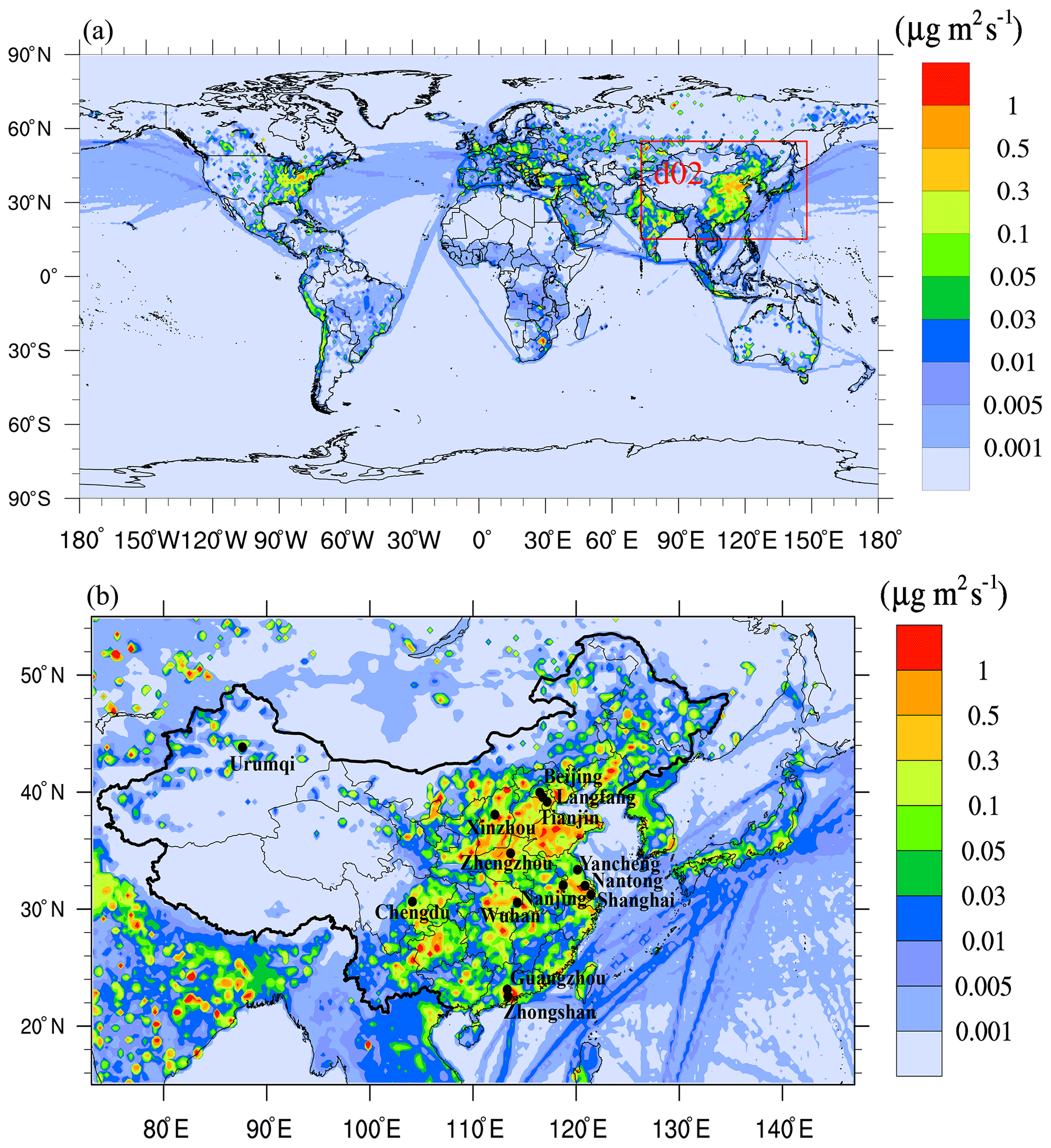
Figure 1The simulation domain showing the total SO2 emissions (µg m−2 s−1). (a) Domain 1, with the position of domain 2 shown using the red square. (b) Domain 2, black circles are locations of the city sites in the domain (China).
2.3 Emissions
By integrating data from publicly released emission inventories, we compiled a global high-resolution () emission dataset with source categories (29 species and 14 sectors) and interpolated it to the model resolution. The benchmark year was 2010. Detailed information on the emissions is shown in Table 1. We note that volcanic emissions are not considered here yet.
Table 1Emissions used in the IAP-AACM. (VOCs refer to volatile organic compounds).

As a consequence of government control policy included in the Five-Year Plan (FYP), China has achieved an obvious decrease in air pollution in the past 10 years, especially for SO2. According to an announcement by the Ministry of Environmental Protection of China (http://www.zhb.gov.cn/gkml/hbb/qt/201507/t20150722_307020.htm, last access: 10 May 2018), the country completed the emission reduction task of 12th FYP (2010–2015) ahead of schedule in 2014 with a reduction ratio of 12.9 %. As the FYP's controls suppressed SO2 emissions mainly in the energy and industry sectors, we adjusted the total SO2 emissions for 2014 by a factor of 0.9 in China. The annual mean SO2 emissions are shown in Fig. 1. According to the latest emission inventory study for China (Zheng et al., 2018), the emissions of other species did not decrease as much from 2010 to 2014. Thus, we did not modify the other emissions.
2.4 Meteorology and evaluation
Meteorological fields were provided off-line by the global WRF. The global WRF is an extension of the mesoscale WRF that was developed for global weather research and forecasting applications. It has a more general choice of map projection (to include both conformal and non-conformal map projections). The specification of planetary constants, physics parameterizations, and timing conventions are also improved to allow the model to be run as a global model. Thus, it has multiscale and nesting capabilities, blurring the distinction between global and mesoscale models and enabling the investigation of coupling between processes at all scales (Richardson et al., 2007). In this study we used WRF version 3.3 (WRFv3.3). The temporal and horizontal spatial resolution of WRFv3.3 was consistent with IAP-AACM. The atmosphere was divided into 27 vertical layers up to 1000 Pa (10 hPa). Output of WRF is interpolated to the vertical layers defined in IAP-AACM. WRF was driven by the National Centers for Environmental Prediction (NCEP) final (FNL) analysis data, and the calculation was nudged to the FNL data.
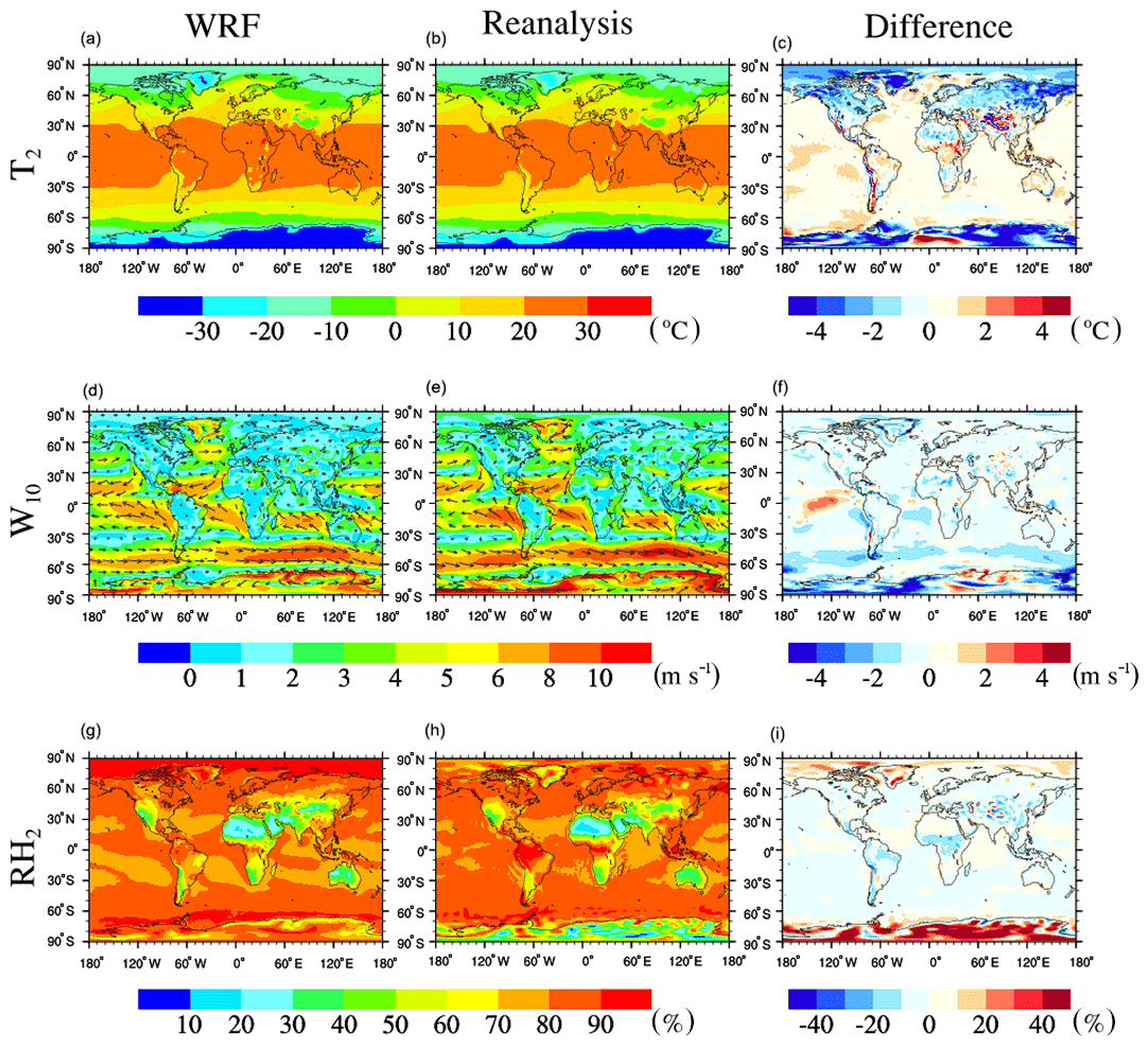
Figure 2Comparison of annual meteorological fields. The left column (a, d, g) is the WRF simulation, the middle column (b, e, h) shows reanalysis data, and the right column (c, f, i) shows the difference between the simulation and reanalysis (WRF–reanalysis). The reanalysis data are NCEP Reanalysis 1.
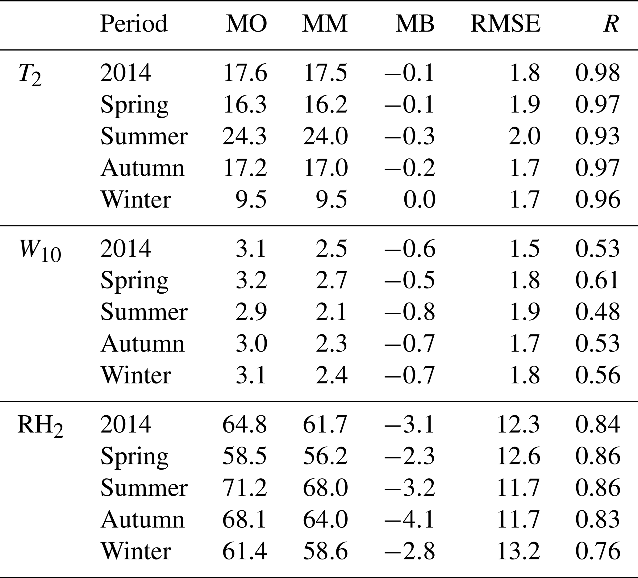
A comparison of annual mean meteorological fields (temperature, wind, and relative humidity) between WRF and reanalysis data (NCEP Reanalysis 1) are presented in Fig. 2. A comparison of annual mean precipitation between the model and reanalysis data from the Global Precipitation Climatology Project is also shown in Fig. S1 in the Supplement. Globally, as shown in Fig. 2, the difference in temperature at 2 m (T2) and wind at 10 m (W10) between the model and observations is within 2∘ and 2 m s−1 respectively, except in high-latitude areas. The relative humidity at 2 m (RH2) is generally underestimated on land and overestimated over the ocean, the difference in most areas is within ±10 %. The difference in precipitation is within 2 mm d−1 except in equatorial regions. The frequently strong convection in tropical areas is difficult to reproduce in the model. A total of 443 surface sites in the nested domain are also analysed with the National Climate Data Center (NCDC) data and the statistical parameters are shown in Table 2. The simulation of the meteorological factors are close to the site records in different seasons, with mean bias (MB) values of −0.3 to 0∘, −0.8 to −0.5 m s−1, and −4 to −2.3 % for T2, W10, and RH2 respectively. The model underestimates T2 in all the seasons, especially in summer with a root mean square error (RMSE) of 2∘. W10 is also underestimated with a MB of −0.8 m s−1. As for RH2, the underestimation is more obvious in summer (MB of −3.2 %) and autumn (MB of −3.2 %) than in spring (MB of −2.3 %) and winter (MB of −2.8 %), which mainly stems from the insufficient prediction of precipitation. The agreement in T2 and RH2 with observations is better than that of W10, with annual correlation coefficients (R) of 0.98, 0.84, and 0.53 respectively. Generally, the meteorology calculated by WRF can rationally reproduce the characteristics of observations.
Table 2Summary of the statistical analysis of annual and seasonal meteorology in the nested domain compared with NCDC sites. Seasons are defined as spring (March–May), summer (June–August), fall (September–November), and winter (December–February). MO, MM, RMSE, and R represent mean value of the observations, mean value of the model, root mean square error, and correlation coefficients respectively. T2, W10, and RH2 represent temperature at 2 m (∘), wind speed at 10 m (m s−1), and relative humidity at 2 m (%) respectively.
2.5 Observation data
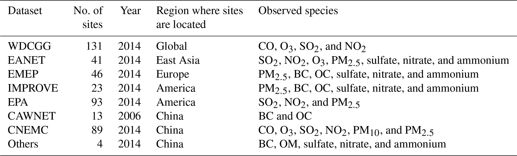
Trace gas observation data for CO, O3, SO2, and NO2 in this paper were collected from the World Data Center for Greenhouse Gas (WDCGG) (http://ds.data.jma.go.jp/gmd/wdcgg/cgi-bin/wdcgg/catalogue.cgi, last access: 20 January 2018), the Acid Deposition Monitoring Network in East Asia (EANET) (http://www.eanet.asia/product/index.html#datarep, last access: 14 June 2019), and the Chinese National Environmental Monitoring Center (CNEMC) (http://www.cnemc.cn, last access: 14 June 2019). Annual observation data of particle and aerosol species are from the European Monitoring and Evaluation Program (EMEP) (http://www.emep.int/, last access: 14 June 2019), EANET, the United States Environmental Protection Agency (EPA) (http://aqsdr1.epa.gov/aqsweb/aqstmp/airdata/download_files.html#Daily, last access: 14 June 2019), and the Interagency Monitoring of Protected Visual Environments (IMPROVE) network (http://vista.cira.colostate.edu/improve/, last access: 14 June 2019). As there are no data published for BC and organic carbon (OC) in Asia in 2014, we collected earlier records from the China Atmosphere Watch Network (CAWNET) reported by Zhang et al. (2008). Hourly air quality data in China were downloaded from CNEMC. The other aerosol observations in China were collected from monitoring sites in Nanjing and Wuhan as well as scientific observations in Xinzhou and Beijing (C. Chen et al., 2015). The aerosol optical depth (AOD) product of MYD04_L2 (https://doi.org/10.5067/MODIS/MYD04_L2.006; Levy and Hsu, 2015) from the Moderate Resolution Imaging Spectroradiometer (MODIS) is used to evaluate the simulated AOD. The total column product from the Global Ozone Monitoring Experiment 2 aboard METOP-A (GOME-2A) (https://www.ospo.noaa.gov/Products/atmosphere/gome/gome-A.html, last access: 14 June 2019) and the Ozone Monitoring Instrument (OMI) (https://earthdata.nasa.gov/earth-observation-data/near-real-time/download-nrt-data/omi-nrt, last access: 14 June 2019) are also used to evaluate the vertical tropospheric column (VTC) of NO2 and O3 respectively. All of these datasets are for 2014, except for CAWNET (which is for 2006). The corresponding simulations at observation sites are sampled at model grid cells containing these sites. The simulations of seasonal cycle in different regions or cities are first sampled at the model grid cells containing the observational sites and then averaged within sub-regions. The observation datasets are summarized in Table 3 and detailed information regarding the observation sites is given in Table S1. Note that the observed species in Table 3 are not always available at the corresponding sites.
To investigate the model performance over China, we selected 89 stations in 12 cities representing typical areas (North China, NC; the Yangtze River Delta, YRD; the Pearl River Delta, PRD; northwest China, NWC; central China, CC; and southwest China, SWC) in China (shown in Fig. 1). The six regions represent the major geographical regions in China, and they are also the regions that severe air pollution research focuses on. The daily mean city-averaged concentration values of pollutants are displayed in figures and are used to calculate statistics. In addition, we collected the mass concentrations of BC, OM, sulfate, nitrate, and ammonium in Beijing, Xinzhou, Nanjing, and Wuhan (shown in Fig. 1) to evaluate the model performance with respect to simulating aerosol components.
3.1 Budgets
On account of the significant radiative effect of sulfate and carbonaceous aerosols, their budgets play an important role in the climate change (Penner et al., 1998). Here we elucidate the budgets of sulfate with its precursor gases (DMS and SO2) and carbonaceous aerosols.
The global budgets for DMS, SO2, and sulfate in the IAP-AACM are summarized in Table 4. For comparison, Table 4 also lists results from other global aerosol models including IMPACT (Liu et al., 2005), the Goddard Institute for Space Studies General Circulation Model with TwO-Moment Aerosol Sectional (GISS-TOMAS) (Lee and Adams, 2010), the Atmospheric Chemistry and Climate Model Intercomparison Project (ACCMIP) models (Lee et al., 2013), and the AeroCom models (Textor et al., 2006). The DMS emissions (23.3 Tg S yr−1) in IAP-AACM are within the range of other models (10.7–22.8 Tg S yr−1). The dry deposition of DMS is zero in the IAP-AACM. Therefore, the sink is only oxidation. This treatment is common in other models such as ModelE2-TOMAS and ModelE2-OMA (Lee et al., 2015). As a result, we have a higher DMS burden of 0.19 Tg S, which is just outside the reference range of 0.05–0.15 Tg S, and a longer lifetime of 3 d. For SO2, the emissions are slightly lower than the reference range (54.3 Tg S yr−1 vs. 63.4–94.9 Tg S yr−1). This is ascribed to the lack of volcanic emissions. The volcanic emissions of SO2 are about 12.5 Tg S yr−1 in most models, based on the work of Andres and Kasgnoc (1998) and Dentener et al. (2006). The oxidation of DMS to SO2 is 22.8 Tg S yr−1, which is within the range of results from other models. The aqueous-phase process is responsible for 61 % of the oxidation to sulfate, and gas-phase processes are responsible for the remaining 39 %. Although it is a slightly lower conversion efficiency for aqueous-phase chemistry compared with other models (about 70 %–80 %), both aqueous-phase and gas-phase oxidation are well within the range of other models. Due to the lower removal in aqueous-phase oxidation (29.8 Tg S) and wet deposition (as zero), the lifetime of SO2 in the model is a little longer than other models (3 d vs. 0.6–2.6 d). In the IAP-AACM, the emission of H2SO4 is assumed to be 2.5 % of the total sulfur emission. With a strong wet scavenging effect, 94 % of sulfate is removed by wet deposition and the rest by dry deposition.
Table 4Global budgets for DMS, SO2, and sulfate.

a Including Liu et al. (2005), Lee et al. (2015), and those listed in
Liu et al. (2005);
the range for sulfate also refers to the GISS-TOMAS (Lee
et al., 2010), the ACCMIP
(Lee et al., 2013), and the AeroCom (Textor et al.,
2006) results.
b Outside the range
of other models.
Table 5 lists the budgets for BC and OM in IAP-AACM. They are within the range of results from other models, including Liu et al. (2005), Lee et al. (2013), Lee et al. (2015), Textor et al. (2006), and those listed in Liu et al. (2005). The emissions of BC and OM are at the low end compared with other models (BC: 7.42 Tg S yr−1 vs. 7.4–19.0 Tg S yr−1; OM: 56.7 Tg S yr−1 vs. 34–144 Tg S yr−1). The ratio of dry deposition to wet deposition for BC and OM is 15.8 % and 13.6 % respectively. Both the burden and lifetime of carbonaceous aerosol are within the results reported by other models. The burdens of BC and OM are 0.13 and 1.16 Tg respectively, and the lifetimes are 6.4 and 7.4 d respectively.
Table 5Global budgets for carbonaceous aerosol.
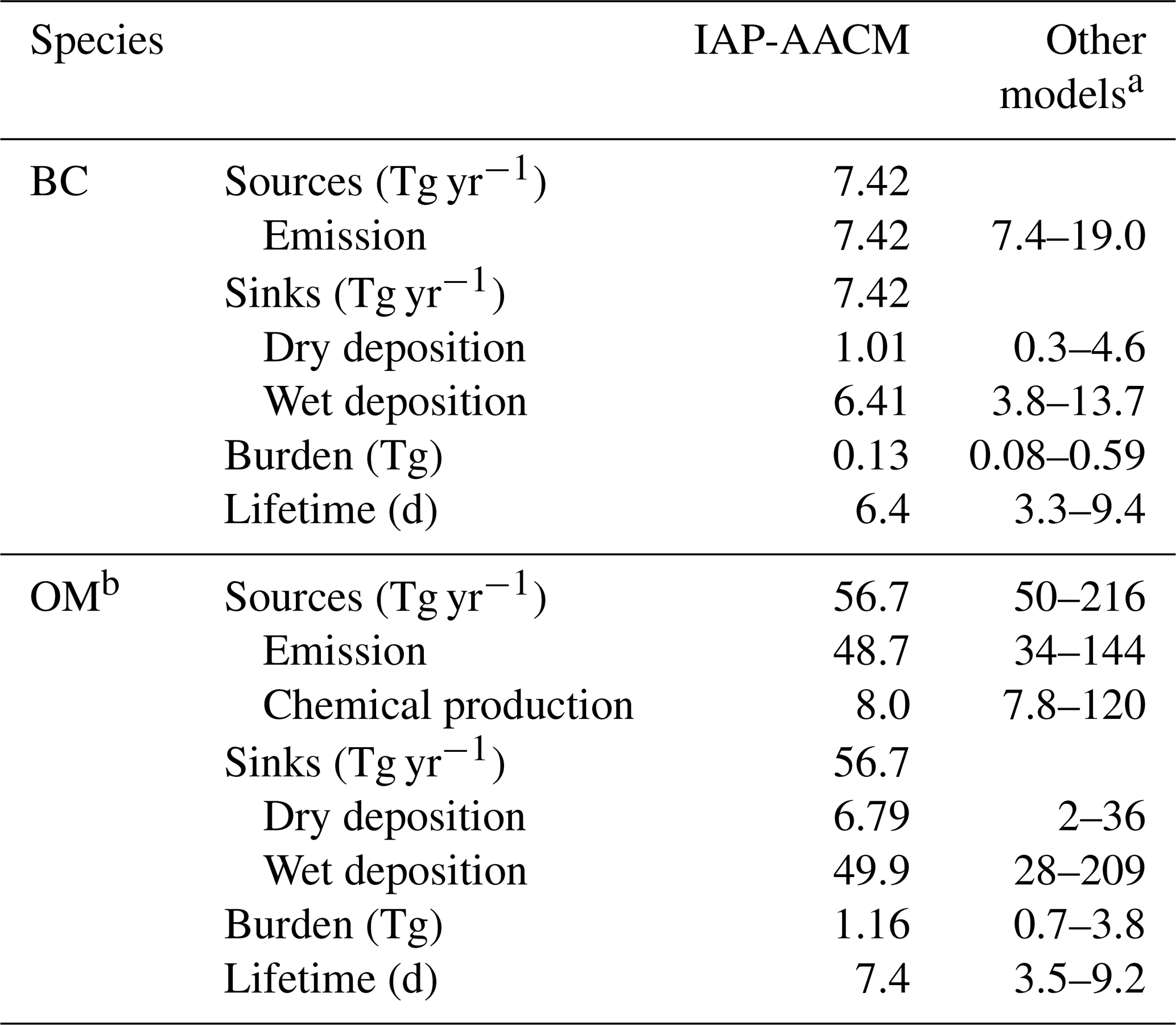
a Including Liu et al. (2005), Lee et al. (2010, 2013, 2015), Textor et al. (2006), and those listed in Liu et al. (2005). b The conversion factor for OC to OM in IAP-AACM is 1.7.
The budgets for CO and O3 are displayed in Table S2. As for CO, the total emissions are 994 Tg yr−1 in IAP-AACM. This is lower than in other models (e.g. 1159 Tg yr−1 in Huijnen et al., 2010, and 1210.7 Tg yr−1 in Emmons et al., 2010). Direct emissions and oxidation contribute 43.4 % and 55.4 % to the total CO respectively. The global annual burden is 327 Tg, which is lower than the value of 353–399 Tg reported in other models (Horowitz et al., 2003; Huijnen et al., 2010; Badia et al., 2017). As for ozone, dry deposition contributes 21.3 % to the total loss (4924 Tg yr−1), and photochemical reaction is responsible for the remaining loss. The dry deposition (1049 Tg yr−1) is larger than values reported by ACCENT and ACCMIP (Young et al., 2018).
3.2 Global distribution and evaluation
3.2.1 Hydroxyl radical (OH)
Oxidation is the basic characteristic of atmospheric chemistry. As the most important oxidant in atmosphere, OH is the crucial species in CTMs. OH in troposphere is mainly produced by the following reaction: . The tropospheric mean concentration of OH in IAP-AACM is 13.0×10⁵ molec cm−3. This is a little higher than the mean OH concentration ( molec cm−3) given by the 16 ACCMIP models in Naik et al. (2013). The high concentration indicates a stronger atmospheric oxidation, which could explain the lower concentration of CO over ocean. The zonal mean OH concentrations for January, April, July, and October are shown in Fig. 3. As in other chemistry models, the OH concentration in the tropics is the highest throughout the year and decreases gradually from the tropics to the poles. This is due to the positive influence of solar radiation and the water vapour concentration. The seasonal north–south shift of the OH maximum is also ascribed to the seasonal variation of these two factors. The mean inter-hemispheric (N ∕ S) ratio of OH in the model is 1.26, which is in accordance with the multi-model mean ratio of 1.28±0.1 (Naik et al., 2013). Vertically, the highest concentration is in the 2–4 km layer over the tropics. In the Northern Hemisphere, the highest OH concentration appears in summer. The peak value is located at around 30∘ N, in the atmosphere above 2 km. Generally, the distribution of the OH concentration is similar to that reported by other models (Huijnen et al., 2010; Badia et al., 2017).

Figure 3Zonal monthly mean concentration of OH in the troposphere for January, April, July, and October from the IAP-AACM (in 105 molec cm−3).
3.2.2 Trace gases
Global annual-averaged surface-layer trace gas distributions from the IAP-AACM are evaluated against site observations in Fig. 4a. Scatterplots of observations and simulations divided into 11 regions are displayed in Fig. 4b. Figure 5 shows the comparison of the annual surface concentrations of CO, O3, and NO2 between IAP-AACM and HTAP CTMs, including CAM-Chem (Lamarque et al., 2012), Oslo CTM3 (Søvde et al., 2012), and CHASER (Sudo et al., 2002).
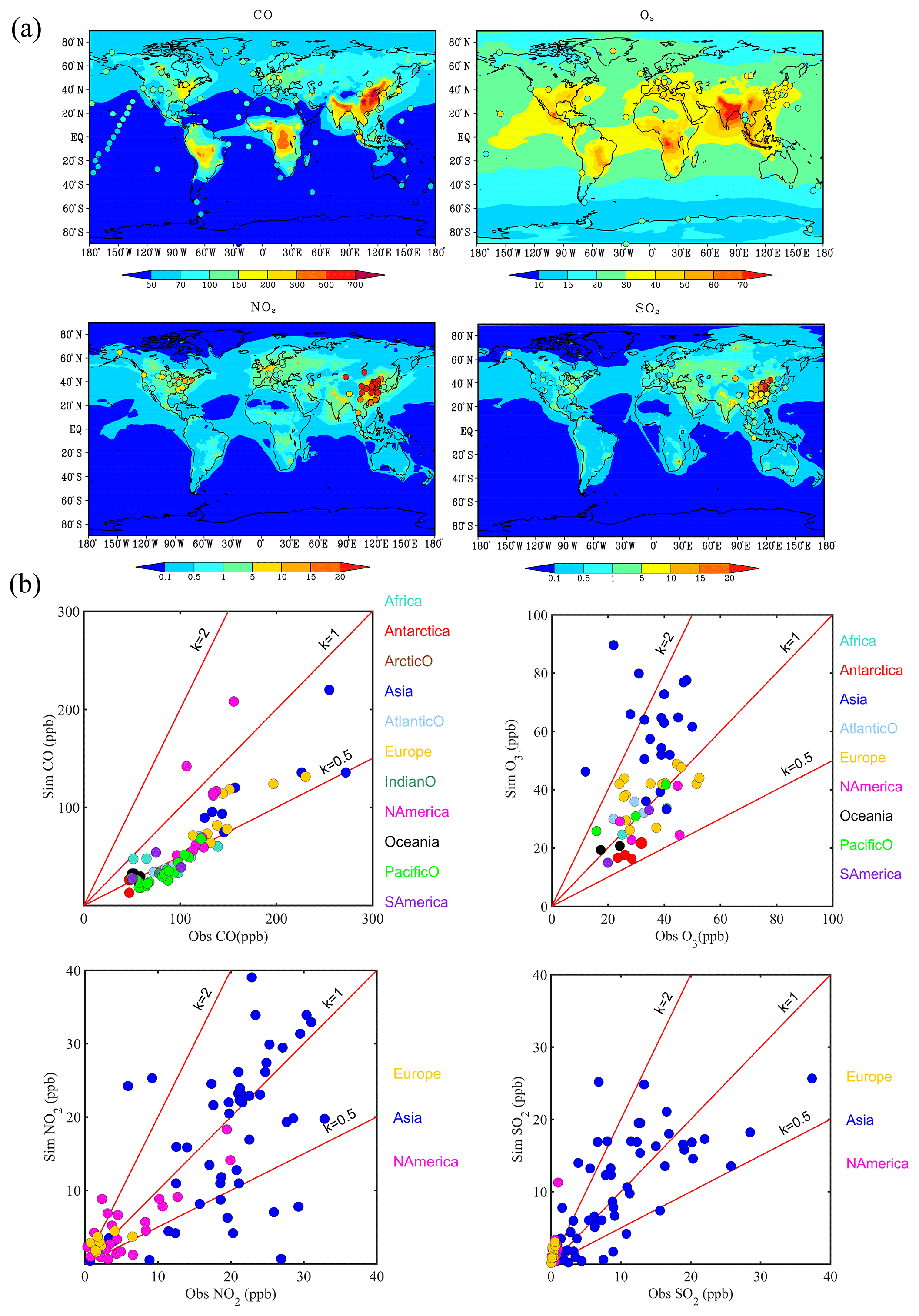
Figure 4Annual mean concentration (ppb) of the surface layer in the IAP-AACM compared with observations. (a) The circles represent site observations. The first row is CO and O3, and the bottom row is NO2 and SO2. (b) Scatterplots for Africa, Antarctica, the Arctic Ocean (ArcticO), Asia, the Atlantic Ocean (AtlanticO), Europe, the Indian Ocean (IndianO), North America (NAmerica), South America (SAmerica), Oceania, and the Pacific Ocean (PacificO). The abscissa shows the observations, and the ordinate shows the simulation. The colour of the points represents different regions.

Figure 5Annual mean surface distributions (ppb) from IAP-AACM compared with HTAP models. Rows from top to bottom represent IAP-AACM, CAM-Chem, Oslo CTM3 and CHASER respectively. The left column displays CO, the middle column displays O3 and the right column is NO2.
Overall, the global surface CO simulation of the IAP-AACM is lower than the observations, especially in natural source regions. The difference over ocean reaches ∼100 ppb, with NMB values ranging from −0.59 to −0.45 (shown in Table S3). In anthropogenic source regions, the model is close to site records in North America (NAmerica), EA, and Europe with NMB values of −0.23, −0.34, and −0.39 respectively. The scatterplot clearly shows a negative bias between the model and observations. The lower model results should be related to underestimated emissions and overestimated OH. As discussed in Sect. 3.2.1, the OH concentration in the troposphere is slightly higher than the other models. As shown in Fig. 3, in the IAP-AACM, the peak concentration of OH (30–35 molec cm−3) is higher than the other models (under 30 molec cm−3). Due to the sink reaction of CO (), the CO loss is larger in the IAP-AACM. Moreover, the anthropogenic emission of CO is 546.4 Tg yr−1 in the IAP-AACM (shown in Table S2). This is lower than other emission inventories (e.g. MOZART-4 with 642 Tg yr−1, Emmons et al., 2010; ACCMIP with 610.5 Tg yr−1, Badia et al., 2017). Janssens-Maenhout et al. (2015) pointed out that CO emission from HTAP_v2 has an uncertainty of 15 %–100 % and 35 %–150 % in data from well-maintained countries and poorly maintained countries respectively. Furthermore, Shindell et al. (2006) evaluated 26 global models and showed that all of the model results were lower than observations in the Northern Hemisphere (NH) except in the tropics. This is related to a lower CO emission source. The spatial distribution of CO concentrations in IAP-AACM is similar to that in other models from HTAP in 2010. High values are found in industrial areas such as North America (NAmerica), Europe, and EA, and biomass burning areas (BBAs) such as South Africa (SAfrica) and South America (SAmerica). Overall, IAP-AACM shows lower concentration in BBAs. This difference probably relates to the different fire emissions used in the IAP-AACM and HTAP models (GFED4 vs. GFED3) (Janssens-Maenhout et al., 2015). Due to the impact of a reduction in combustion area and decreasing fuel consumption, there is a reduction of about 20 %–30 % in BBAs for CO emissions in GFED4 compared with GFED3 (van der Werf et al., 2017).
The surface distribution of O3 simulated by the IAP-AACM is in a good agreement with observations. The O3 simulations at most sites are within a factor of 2 of observations, and all the regions have NMB values within ±0.2 (Table S3) except for Antarctica and Asia. There are three sites in Southeast Asia that exhibit concentrations more than twice the observed values. As these sites are located at the coast, simulations in the coarse grids cannot capture the steep variation. Additionally, South Asia is a high-emission area for biogenic volatile organic compounds (VOCs). Uncertainties in the biogenic emission inventory also cause large errors in the O3 simulation due to photochemical processes. As shown in Fig. 5, the IAP-AACM exhibits a generally similar surface distribution of O3 to the other models. However, the model shows lower concentrations in high-latitude areas (especially over ocean) than the other models. That could be partly related to the dry deposition over sea ice. The dry deposition velocity to ice is under 0.02 cm s−1 across the 15 HTAP models (Hardacre et al., 2015). In the IAP-AACM, it is higher (0.035–0.048 cm s−1) than in the abovementioned models, as shown in Fig. S2. Additionally, the dry deposition velocity over ocean is 0.042–0.05 cm s−1 in IAP-AACM compared with the HTAP models (around 0.05 cm s−1); according to Ganzeveld et al. (2009) there should be a difference of less than 12 %.
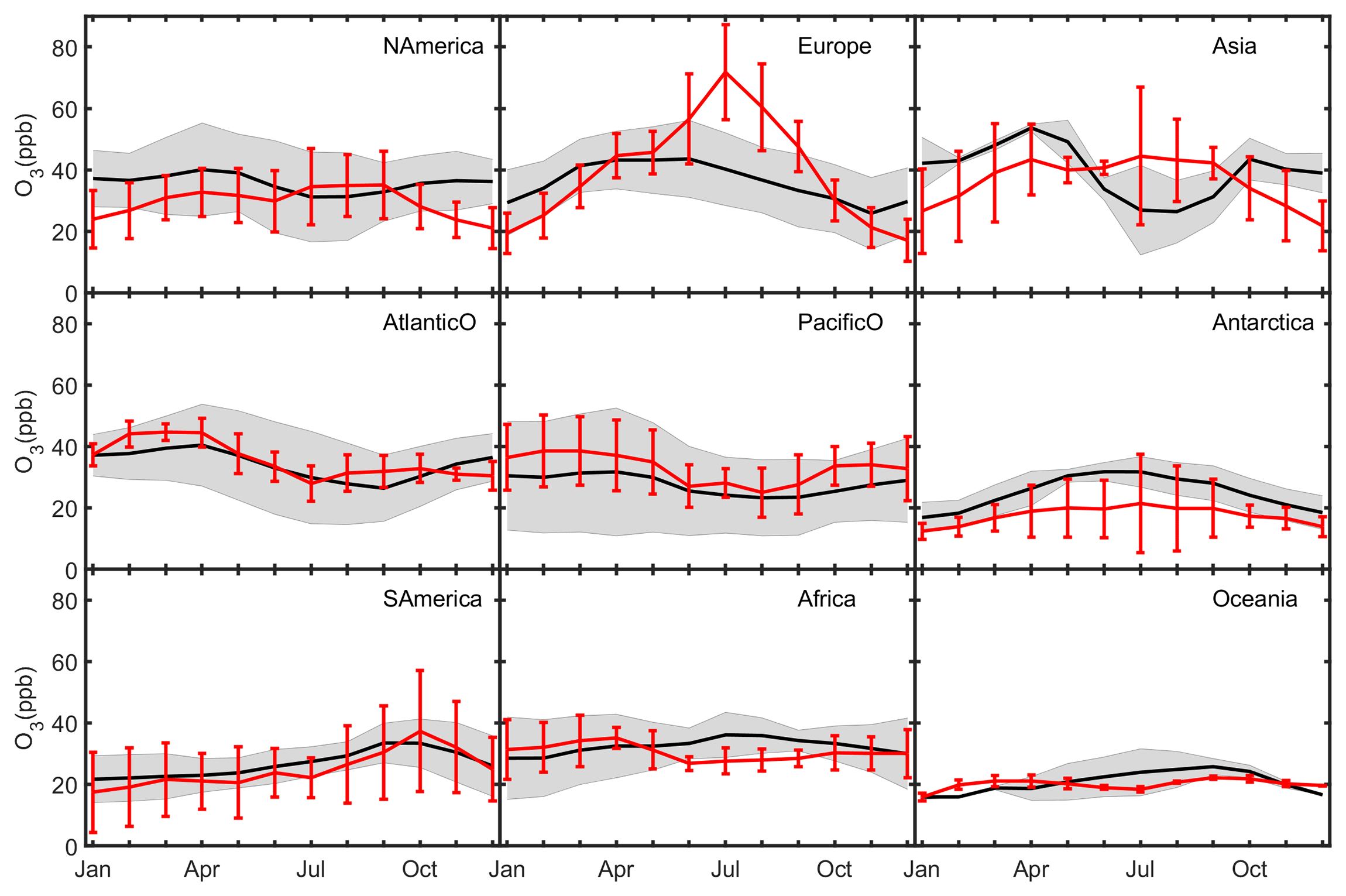
Figure 6Mean seasonal variation of O3 (in ppb) over the NAmerica, Europe, Asia, AtlanticO, PacificO, Antarctica, SAmerica, Africa, and Oceania sites. Black and red lines represent the average of observations and simulations respectively. Grey shaded areas and red vertical bars show ±1 standard deviation for observations and for model results respectively.
As shown in Fig. 6, the model shows good skill in capturing the seasonal variation of surface O3 in the Southern Hemisphere (SH) and NH oceans. Over ocean, the O3 concentration is higher in spring and lower in summer. In contrast, it is higher in autumn or summer over land in the SH. The model shows poor performance regarding the seasonal cycle of surface ozone in the NH, with an underestimation in the NH over land in cold seasons and an overestimation in Europe and EA in summer. In the IAP-AACM, the stratospheric–tropospheric exchange is not considered. This leads to a large negative bias in the simulation. The stratosphere-to-troposphere ozone transport event occurs widely across mid-latitudes in the NH (Monks, 2000; Akritidis et al., 2018). Research (Munzert et al., 1985; Austin and Follows, 1991) has shown that the maximum stratosphere to troposphere flux occurs in late winter/spring. The surface O3 concentrations over EA (sites mainly located in Japan) are overestimated in summer and early autumn. The same pattern is also found in the multi-model inter-comparison of 21 HTAP models (Fiore et al., 2009). The simulations in island countries located in EA are sensitive to the timing and extent of the Asian summer monsoon (Han et al., 2008). The positive model bias in this season may stem from an inadequate representation of the southwesterly inflow of clean marine air. Furthermore, the underestimation of cloud cover in summer may also be responsible for the overestimation of O3 due to stronger photochemistry. Additionally, it is difficult for a global model with a coarse resolution to resolve local orographically driven flows or sharp gradients in mixing depths under complex underlying surface conditions over land. As the seasonal variation of surface O3 should be different in different environments, a seasonal cycle comparison between these NH sites which are separated into land, mountain, and marine is also shown in Fig. S3. The underestimation in cold seasons and overestimation in summer are found in different environments to varying degrees. For inland areas, the model tends to overestimate O3 concentrations in summertime. Uncertainties in VOC–NOx–O3 chemistry may also contribute to this overestimation. The natural source of isoprene from vegetation is important regarding O3 formation due to its high proportion of VOC emissions in summer (estimated to be 40.9 Tg yr−1 in China by Fu et al., 2012). In IAP-AACM, the O3 concentration is about 5–15 ppb lower than site observations in Antarctica. This may be caused by the lack of halogen chemistry in the model. Remarkable ozone depletion events driven by halogen chemistry (mostly notably as bromine) are observed in the polar boundary layer (Simpson et al., 2007). A model study by Falk and Sinnhuber (2018) indicated that there are missing sources of bromine release from ice and snow in EMAC v2.52. The over-prediction of dry deposition velocity to sea ice also plays a role here, as previously mentioned.
NO2 is mainly distributed in the anthropogenic source areas, which is well captured by IAP-AACM (see Fig. 4a). In the NH, the maxima are located in urban areas due to fossil fuel combustion from traffic and industry. The surface concentration of NO2 is much higher in eastern China (>20 ppb) than in eastern NAmerica and Europe (3–10 ppb). In the SH, the maxima are located in SAmerica and SAfrica due to biomass burning, where NO2 ranges from 1 to 10 ppb. The simulations are in good agreement with observations in NAmerica, Europe, and most parts of EA. As shown in Fig. 4b, simulations are within a factor of 2 of observations at most sites, with NMB values of −0.14, 0.16, and −0.14 for Asia, Europe, and NAmerica respectively. As we use the same anthropogenic emission inventory, the distribution of NO2 in the NH between IAP-AACM and other models is similar (shown in Fig. 6). The concentrations in SAmerica and SAfrica are slightly lower (∼3 ppb) than in the other models, due to the aforementioned different version of GFED data used in the IAP-AACM and HTAP models. Compared with the other models, the surface NO2 over ocean is higher in IAP-AACM. In IAP-AACM, the emissions of energy and industry are emitted in the first five layers considering the stack height. The higher injection height of emissions leads to a larger transportation distance and lower NOx at the surface in source areas (Badia et al., 2017). Consequently, it also leads to a higher concentration of surface ozone in NH source areas due to weak NOx titration.
Similar to NO2, SO2 shows high values in the NH over land, mainly due to human activities associated with fossil fuel combustion. Maximum concentrations are mainly found in NAmerica, Europe, India, and EA, ranging from 5 to 20 ppb; concentrations can even reach over 20 ppb in eastern China. SO2 over ocean is mainly due to DMS oxidation from marine organisms, ranging from 0.1 to 1 ppb. The model shows a distribution of 0.1–20 ppb in EA and 0.1–5 ppb in western NAmerica, which is consistent with observations. The simulated values of SO2 in eastern NAmerica and Europe are about 1–10 ppb and are overestimated, with NMB values of 3.51 and 3.79 respectively (as shown in Table S3).
3.2.3 Aerosol composition
Figure 7 shows the annual surface concentrations of aerosols in IAP-AACM in comparison with site observations. The formation of sulfate, nitrate, and ammonium (SNA) are due to gas-to-particle conversion in the atmosphere. The distribution of SNA is consistent with the precursor gases (SO2, NOx, and NH3), mainly in the NH over land. As shown in Fig. 7a, the surface distribution of SNA in IAP-AACM is generally close to the site records. As shown in Fig. 7b, sulfate is more or less overestimated. Specifically in Asia, the simulations at most sites are within a factor of 2 of observations, with a NMB of 0.36. However, in NAmerica and Europe, it is overestimated with NMB values of 1.94 and 1.1 respectively. The site-averaged simulation value is 1.67 and 1.56 µg m−3 higher than observations in NAmerica and Europe respectively. This overestimation is consistent with the high level of SO2 described previously. There are more uncertainties in the simulation of nitrate, as the volatility of HNO3 makes nitrate formation more sensitive to environmental factors such as temperature and relative humidity in the atmosphere. The complex photochemical reactions of NOx also contribute to the uncertainties. The concentration of nitrate is higher in eastern America and lower in western America. IAP-AACM reproduces the distribution of nitrate in western America well but overestimates it in eastern America. The model does not fully capture the spatial variation over Europe, with an overestimation at most of the sites. For EA, there is an underestimation of ∼5 µg m−3 in Southeast Asia and Japan. Overall, the NMB values are within ±0.8 (0.5, 0.74, and −0.61 for NAmerica, Europe, and EA respectively). The performance of ammonium varies in different regions, as there are more uncertainties in the emission of NH3 (the precursor of ammonium) from croplands (Xu et al., 2019). There is slight negative bias in America and a positive bias in Asia, with NMB values less than ±1 (−0.46 and 0.85 respectively). In Europe, there is a significant positive bias with a NMB of 1.49.
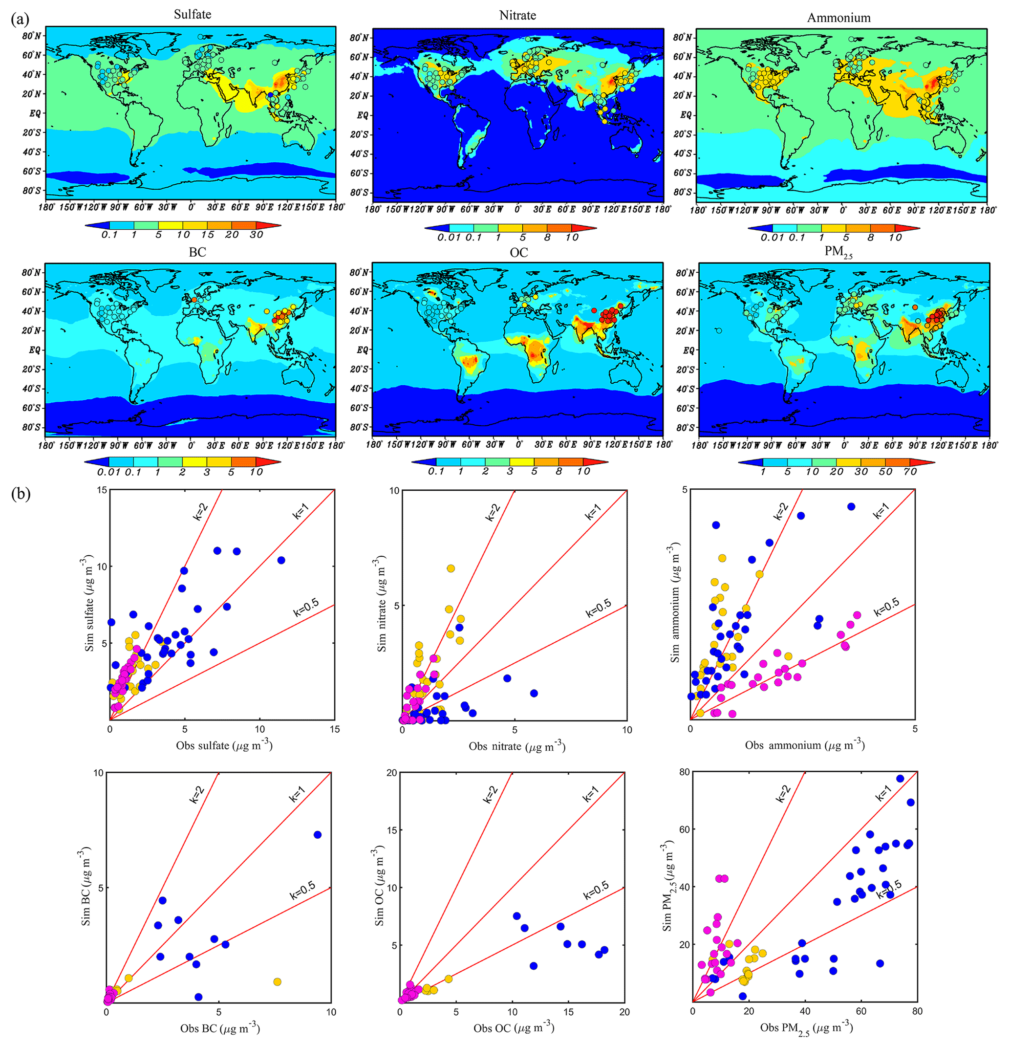
Figure 7(a) The same as Fig. 4, except for sulfate, nitrate, ammonium, BC, OC, and PM2.5 (in µg m−3). The top row is sulfate, nitrate, and ammonium, and the bottom row is BC, OC, and PM2.5. (b) Scatterplot of annual mean concentration. The order of the plots in (b) are in accordance with panel (a). Solid circles in blue, yellow, and magenta represent Asia, Europe, and NAmerica respectively.
Due to the large contribution of biomass burning and fossil fuel combustion associated with old technology, carbonaceous aerosols are higher in developing countries than in developed regions such as NAmerica and Europe. The concentration of BC and OC ranges from 2 to 10 and 5 to 10 µg m−3 in China and India respectively, whereas it ranges from ∼1 and 3 to 10 µg m−3 respectively in SAfrica and SAmerica. In general, the model results are consistent with observations in the three regions shown in Fig. 7, with NMB values within ±0.65 and ±0.7 for BC and OC respectively. The accuracy of the simulation mainly depends on emissions and deposition processes, as BC is quite inert to chemical reactions.
The simulation of BC in China is accurate with 70 % of the stations within a factor of 2 of observation, whereas OC is underestimated by about 5–10 µg m−3. The meteorological conditions and emission inventories in the model are inconsistent with the observation year (2006) of carbonaceous aerosols in China. This may be partially responsible for the bias of OC. According to recent studies, there was a slight increase (less than 0.1 Tg) in both BC and OC emissions from 2006 to 2010 in China (Lu et al., 2011; Fu et al., 2012). As shown in Fig. 7, the simulated BC concentrations at most sites are close to observations, whereas the simulated OC is significantly underestimated. The study by Fu et al. (2012) showed a significant underestimation of OC emissions over China. Furthermore, Zhao et al. (2016) found that the pathway of intermediate volatile organic compounds (IVOC) to SOA is very important regarding the formation of SOA. Their model experiments suggested that IVOCs constitute over 40 % of the OM concentrations in eastern China. Yang et al. (2018) also showed a significant increase in the SOA concentration in an observation-based box model which included IVOC reactions. IVOC reactions are not included in our SOA module. The SOA module in IAP-AACM is a two-product scheme. Model studies using a two-product scheme estimated an underestimation of OM by 40 %–78 % in China (Lin et al., 2016; Han et al., 2016). Thus, the close simulation of BC but large underestimation of OC calls for an improvement in the SOA formation mechanism in IAP-AACM.
Generally, the model shows good skill in simulating PM2.5. Model results at most sites are close to observations, as shown in Fig. 7b, especially in Europe and Asia with NMB values of −0.35 and −0.36 respectively. The underestimation in western China could be related to uncertainties in emissions and unrepresentative simulation with coarse grids.
3.2.4 Comparison with satellite data
The VTC of O3 is compared against satellite observations derived from OMI (shown in Fig. 8). In general, the pattern of the seasonal cycle was covered by the model. On the Northern Hemisphere mainland, higher O3 VTC appears during June–July–August (JJA), whereas in the SH it appears during September–October–November (SON) with a range of 40–60 DU. The model maintains a high value (40–50 DU) in the tropics during December–January–February (DJF), which is possibly due to the high concentration of CO emitted from biomass burning. The underestimation of cloud cover in the intertropical convergence zone may also contribute. The O3 VTC is significantly underestimated over ocean in middle–high latitudes. As the stratospheric chemistry is not considered in IAP-AACM, the lack of stratospheric–tropospheric exchanges could partly be responsible for the underestimation of the column burden.

Figure 8Seasonal mean column concentration of O3 from IAP-AACM (left column) and OMI (right column). Seasons are defined as March–April–May (MAM), June–July–August (JJA), September–October–November (SON), and December–January–February (DJF).
The VTC of NO2 is also compared against satellite observations derived from GOME-2A (shown in Fig. 9). The NO2 VTC has a range of 20–150×1014 molec cm−2 in most source areas. In general, IAP-AACM reproduced the magnitude in different regions. In addition, the model captured seasonal variations in the NO2 concentration in the vertical troposphere well. In anthropogenic source areas in the NH (e.g. NAmerica, Europe, and EA), the NO2 VTC is higher in SON and DJF and lower in JJA. The column concentration is higher during JJA in SAmerica and SAfrica, whereas it is higher during DJF in central Africa due to vegetation burning in dry season. Compared with GOME-2A, IAP-AACM showed a larger column concentration over ocean. The overestimation is also reflected in the comparison of the surface concentration. This is probably caused by insufficient oxidation to nitrate and a higher injection height of emissions which leads to a larger transportation distance, as suggested in Badia et al. (2017). Generally, the distribution of tropospheric NO2 by the model is consistent with satellite observations.
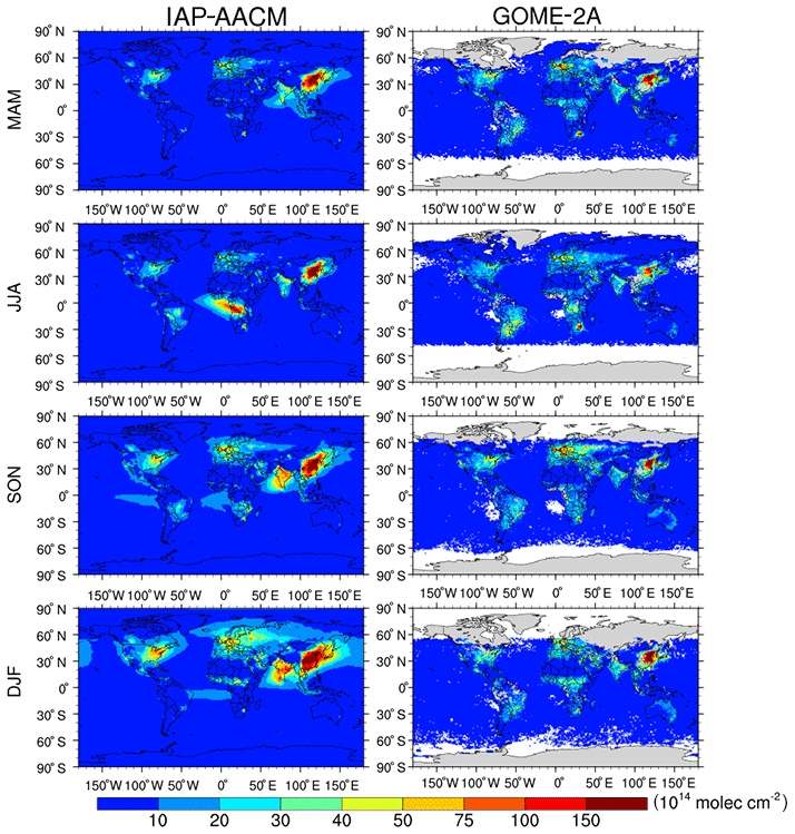
Figure 9Seasonal mean column concentration of NO2 from IAP-AACM, left column, and GOME-2A, right column (in 1014 molec cm−2).
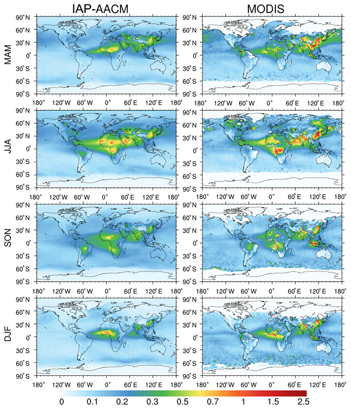
In order to evaluate the column burden of aerosol in IAP-AACM, we compared the AOD from IAP-AACM with MODIS satellite data as shown in Fig. 10. The calculation of the light-extinction coefficient, bext550 (1 Mm−1 at 550 nm), follows Eq. (1) given by Li et al. (2011):
where fSNA (RH) and fSS (RH) represent the hygroscopic growth factor for SNA and sea salt respectively, and the variables in brackets are the mass concentration of aerosol species (OC – organic carbon, BC – black carbon, FD – fine dust, CD – coarse dust, and SS – sea salt).
In Fig. 10, the model reproduces the spatial features of AOD exhibited by satellites globally. For example, the high value around 60∘ S, ranging from 0.1 to 0.3, is due to high concentrations of sea salt. The maximum in SAmerica and SAfrica is due to the large amount of carbonaceous aerosol produced by biomass burning. The desert maximum over 0.5 is caused by mineral dust in NAfrica, Arabian Peninsula, and western China. High AOD in NAmerica, Europe, India, and EA is caused by anthropogenic aerosols. Furthermore, there is a good agreement of the seasonal variations with satellite observations. For example, the AOD in the desert areas of the NH reaches a maximum in March–April–May (MAM), as there are frequent dust storms during this period. SAmerica and SAfrica exhibit the highest AOD during JJA as more biomass burning takes place in this season. However, there are several biases between the model and observations. The model shows a weaker AOD in Southeast Asia than the observations, where the value is mainly controlled by biomass burning. The AOD from IAP-AACM is lower than observations by about ∼0.4 in eastern China, which is mainly due to the negative bias in anthropogenic aerosols simulation. Furthermore, the underestimation of RH2 in eastern China (shown in Fig. 2) is also responsible for the lower simulation of AOD. The comparison of monthly gridded average AOD (shown in Fig. S4) shows a discrepancy in EA, due to the bias of dust simulation in spring.
3.3 Nested simulation evaluation
3.3.1 Distribution of pollutants in EA
Figure 11a shows the annual distribution of the four pollutants SO2, NO2, PM10, and PM2.5, against 45 city stations from the nested simulation. In general, the simulation shows better agreement with sites in eastern China than in western China. The distribution of PM2.5 and its precursors shows high levels in eastern China and low levels in western China, which is related to large emissions in the east. The simulation is in good agreement with observations at most sites. Concentrations of precursor gases and particles in Tibet are greatly underestimated, as the model's coarse resolution cannot represent the emission for the region. As shown in Fig. 11b, model results for NO2, SO2, and PM2.5 are mostly within a factor of 2, with NMB values within ±0.3. The “NO2” values reported by routine monitoring sites are , which partially includes HNO3 and . This implies that the model may overestimate “NO2”. PM10 concentrations are underestimated at all sites with a NMB of −0.51. The model results for PM10 and PM2.5 include primary PM2.5, BC, POA, SOA, and SNA. As natural dust contributes a lot to particles in Northwest China, it is underestimated in this area.
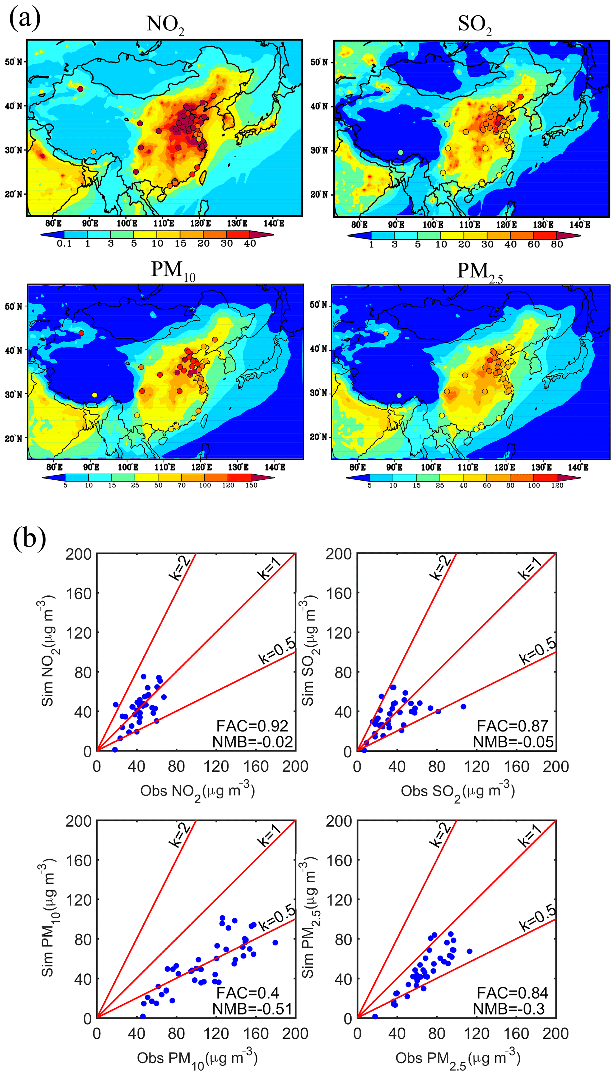
Figure 11(a) Surface annual mean concentration of the nested domain (in µg m−3). The circles represent sites observations. The top row is NO2 and SO2, and the bottom row is PM10 and PM2.5. (b) Scatterplots of annual mean concentrations in the nested domain (in µg m−3). The order of the panels (b) are in accordance with the order in panel (a). The abscissa shows the observations and the ordinate shows the simulation.

Figure 12Annual surface distributions from the nested IAP-AACM compared with regional models from MICS-Asia. Each row from top to bottom represents IAP-AACM, WRF-Chem, CMAQ, and NAQPMS respectively. The left column is SO2 (ppb), the middle column is NO2 (ppb), and the right column is PM2.5 (µg m−3).
Model inter-comparison can give some insights into model uncertainties. Here a comparison between IAP-AACM and several regional models of MICS-Asia is presented (Fig. 12). The MICS-Asia models shown here are WRF-Chem(v3.9; Tuccella et al., 2012), CMAQ(v4.7.1; Mebust et al., 2003), and NAQPMS (Wang et al., 2006b). The simulations are for 2010 with the same meteorological fields, emissions, and horizontal resolution (45 km). Overall, the IAP-AACM shows a similar annual distribution to the MICS-Asia models in EA, as the emission inventories used in IAP-AACM are largely the same as for the MICS-Asia models. The simulation of SO2 in IAP-AACM is similar to WRF-Chem and CMAQ. The simulation of NO2 in IAP-AACM is lower in source areas (e.g. eastern China and Japan) but higher over downwind areas compared with CMAQ. This is possibly related to the higher injection height in IAP-AACM. Although the models use the same dynamic framework, SO2 and NO2 in IAP-AACM are lower than in NAQPMS. This could be related to the different dry deposition schemes used by as Zhang et al. (2003) and Wesely (1989) in IAP-AACM and NAQPMS respectively. Furthermore, the PM2.5 from NQAPMS is higher than in IAP-AACM in northwest China, as it includes dust aerosol in NQAPMS. Overall, the simulation in the nested domain of the global model is comparable to the regional model.
3.3.2 Trace gas evaluation in cities
To gain deeper insight into the performance of IAP-AACM in cities, the nested simulation was compared with daily averaged observations in 12 cities across China. We first focused on NO2 and SO2, as they are precursors of SNA aerosols. The monthly variation of SO2 and NO2 against observations is shown in Figs. 13 and 14. Three-quarters of cities show an annual concentration of SO2 of around 25 µg m−3, which is only half of the NO2 concentration in summer and autumn owing to the strict SO2 emission reduction policy that has been implemented since 2005. For SO2, the model shows good agreement with observations except in Wuhan. This probably implies an overestimation of emissions in this city. Furthermore, IAP-AACM reproduces the seasonal variation well, showing good comparison to observations with R values over 0.5 in most cities, as shown in Table 6. In particular, the cities in NC have a high R values of between 0.76 and 0.89.
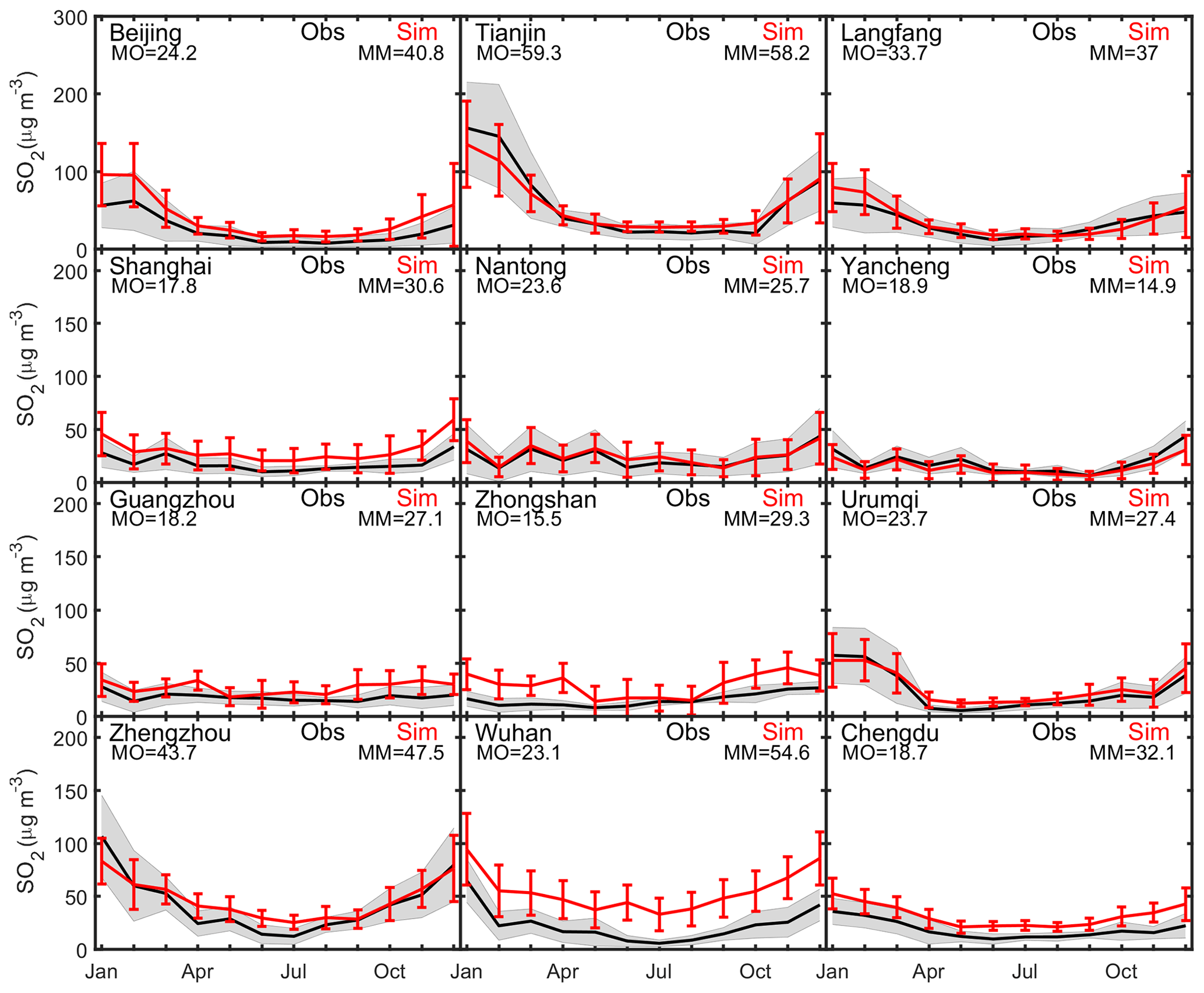
Figure 13Mean seasonal variation of SO2 (µg m−3) over China. The black and red lines represent the monthly mean concentration of the city-averaged observations and simulation respectively. Gray shaded areas and red vertical bars show ±1 standard deviation over the sites for the observations and for model results respectively. MO and MM represent the annual mean concentration of the observations and simulation respectively.
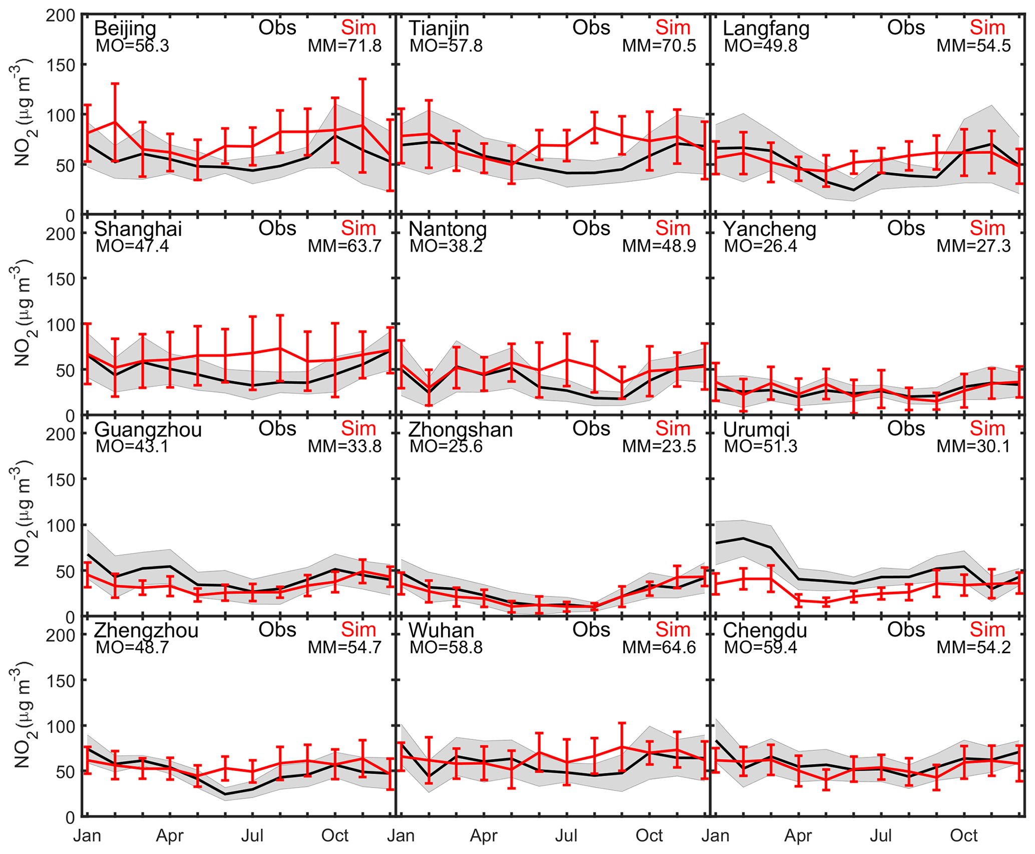
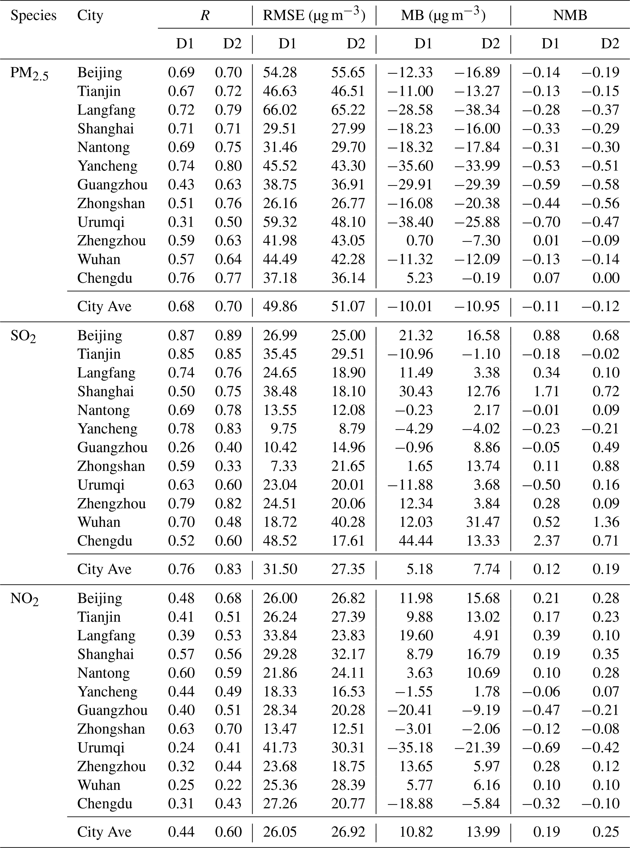
Table 6Summary of the statistics for the global and nested domains. D1 and D2 represent the results for domain 1 and domain 2 respectively. “City Ave” refers to the average of all cities.
As illustrated in Fig. 14, the model shows good performance for NO2 in cities in the PRD and SWC, matching observations well with RMSE values of less than 20 µg m−3. The model captures the daily variations well with R values of between 0.49 and 0.7 in NC, the YRD, and the PRD. However, the model overestimates NO2 in NC, the YRD, and CC in summer. The overestimation of NO2 in summer is associated with deposition removal process and multiphase chemistry in IAP-AACM. The overestimation of NO2 and the underestimation of nitrate in daytime in summer and autumn relates to the over-decomposition of nitric acid (HNO3) under high-temperature conditions in the thermodynamic equilibrium module. Moreover, heterogeneous chemical reactions in the model could be partly responsible for the overestimation in summer. The heterogeneous chemical module coupled in IAP-AACM has been applied in North China in winter (Li et al., 2018). The mechanism significantly improved sulfate simulation under highly polluted conditions (contributing 50 %–80 % of the total concentration of sulfate) and reduced the overestimation of nitrate. However, the simulations that excluded heterogeneous chemical processes showed better performance for NO2 (shown in Fig. S5). This indicates that a more reasonable mechanism should be considered in model development. Here we also give a comparison of NO2 VTC over the nested domain between IAP-AACM and GOME-2A in Fig. S6. Generally, the model captures seasonal variations of NO2 VTC well. In China, the NO2 VTC is higher during SON and DJF and lower in JJA due to unfavourable diffusion conditions and weaker photochemical reactions in autumn and winter.
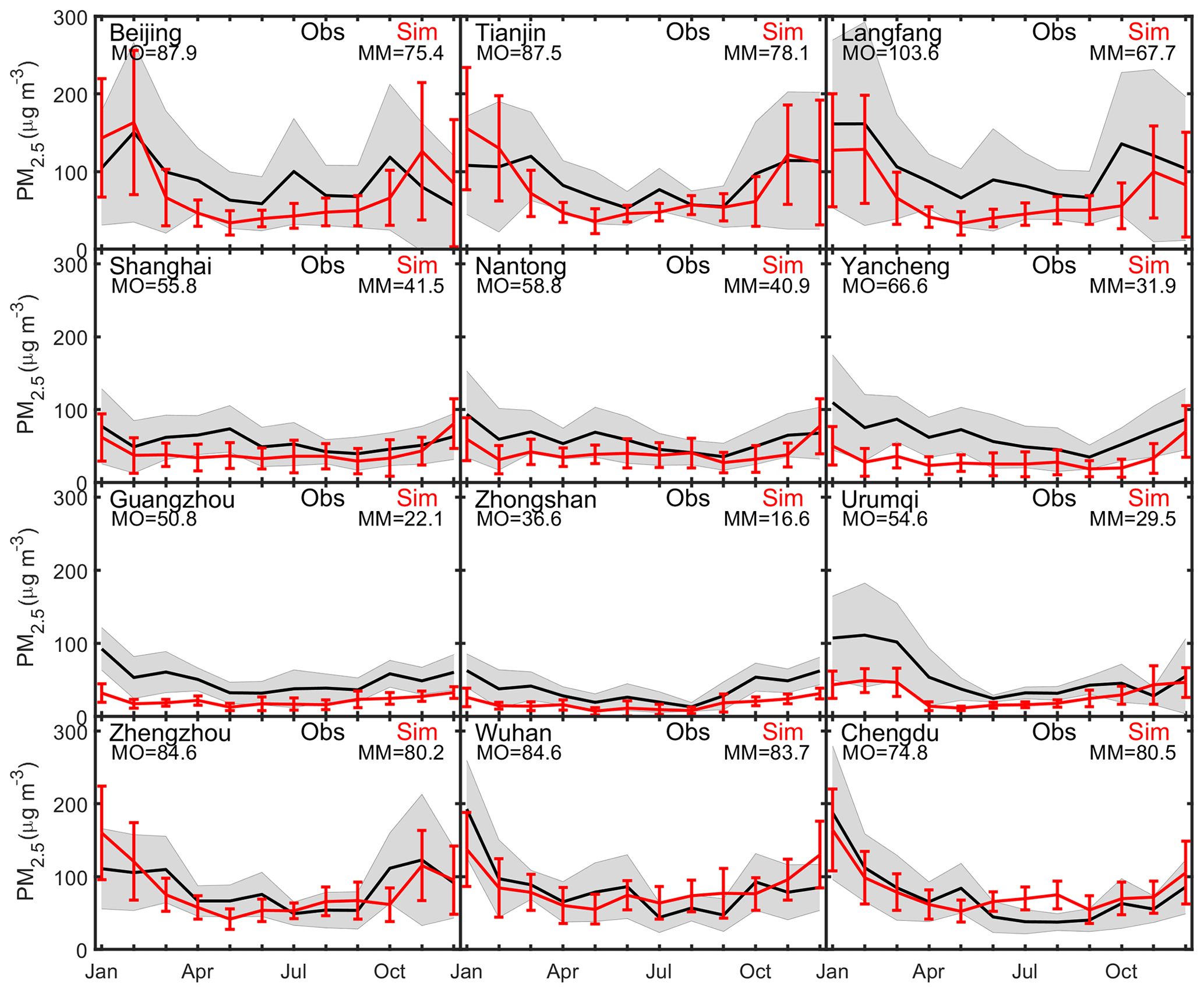
Figure 15The same as Fig. 13 components of PM2.5 include primary PM2.5, BC, POA, SOA, and SNA.
3.3.3 Aerosol composition evaluation in cities
As shown in Fig. 15, the model performs very well regarding the simulation of PM2.5. The model reproduces PM2.5 variation over the 12 cities well, particularly in NC, the YRD, and SWC, with an R of 0.70–0.79, 0.71–0.80, and 0.77 respectively. The model results are close to or slightly lower than site observations with a city averaged NMB of −0.12. The concentration in NC on winter days is below the observations. Underestimation of PM2.5 in severe haze periods is common in CTMs, mainly as a result of the deficiency in the simulation of SNA and SOA (Zheng et al., 2015; Donahue et al., 2006). Additionally, the simulation of meteorology (e.g. RH, wind speed, and planetary boundary layer height) is more uncertain during severe haze periods. There is a clear underestimation in the PRD and Urumqi, where mean values are less than half of the observations, with a NMB around −0.5. In the PRD, it could be related to the underestimation of precursor emissions and the decomposition of HNO3. In Urumqi, it could be more closely related to the unrepresentative simulation with coarse grids. Compared with the scale of urban areas and local emissions in Urumqi, the model grid area is too large. Thus, the averaged value of grids is significantly lower than the local site records. Furthermore, dust is an important component of PM2.5 in Urumqi, and this is not included in the result.
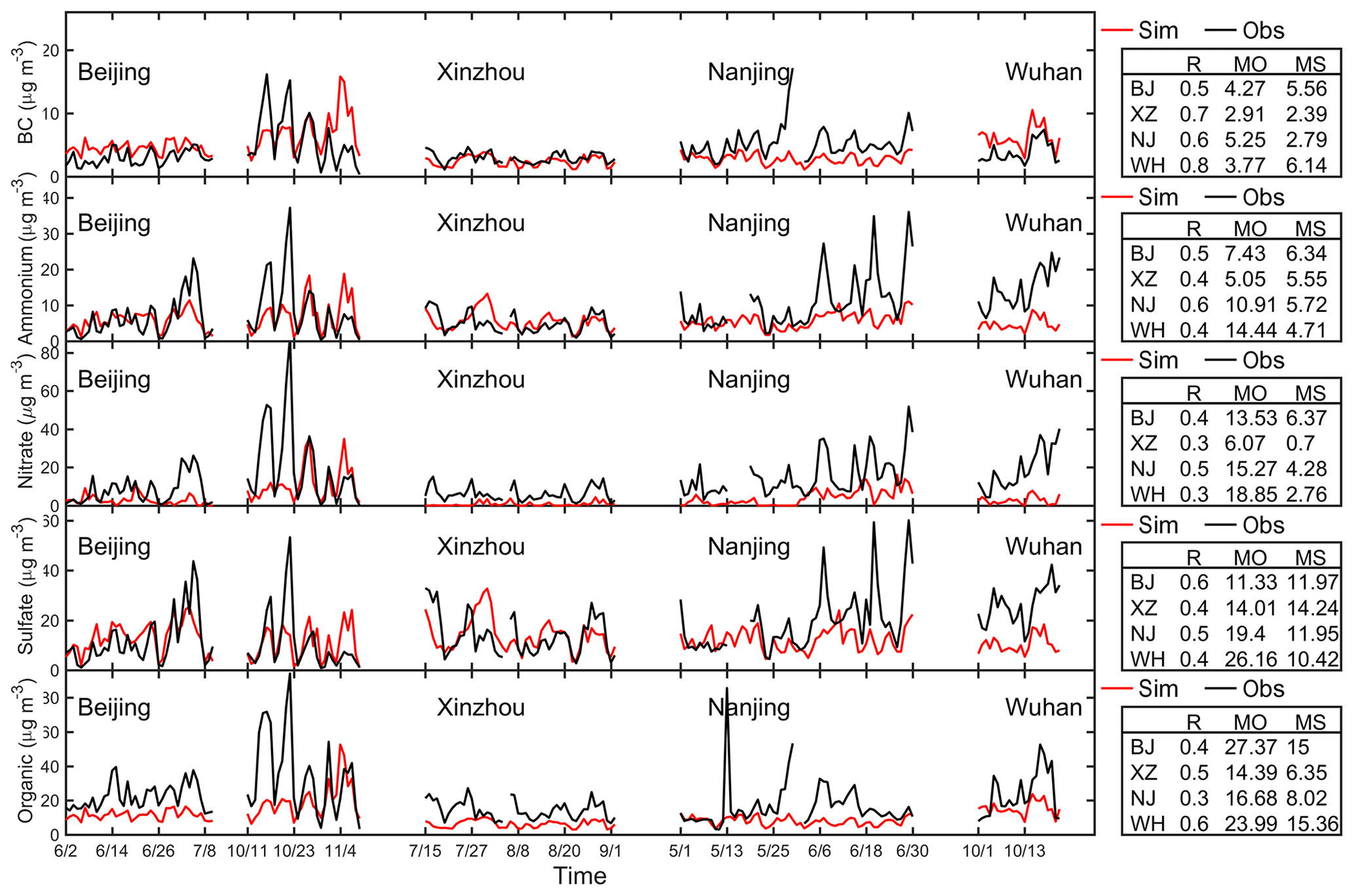
Figure 16Daily variation of aerosol components (µg m−3) over China. The black and red lines represent the daily mean concentration of the city-averaged observations and simulation respectively. BJ, XZ, NJ, and WH refer to Beijing, Xinzhou, Nanjing, and Wuhan respectively. R, MO, and MM stand for correlation coefficient, mean concentration of observation, and mean concentration of model respectively. (“Organic” on the y axis of the lower panel refers to organic matter.)
To assess the performance of IAP-AACM with respect to representing aerosol components, we compare the model results with four stations in NC, the YRD, and CC in Fig. 16. Generally, the model represents the variation of BC well with R values ranging from 0.5 to 0.8 – the values are close to observations. As a primary species, the simulation of BC depends on the emission inventory and meteorological conditions. Unlike BC, OM is underestimated at these stations, with a negative bias of 8–12 µg m−3. For SNA aerosols, sulfate is close to observations in the northern cities (Beijing and Xinzhou), but is underestimated by about 10 µg m−3 in southern and central cities (Nanjing and Wuhan). As the concentration of SO2 in Wuhan is overestimated, this suggests an underestimation of transportation or the insufficient oxidation of sulfate; the insufficient conversion of sulfate has been discussed widely in recent years (Cheng et al., 2016; He et al., 2014). Moreover, SO2 emitted by coal power plants plays a vital role in the formation of sulfate. The coarse grid resolution is insufficient to reproduce the rapid conversion of H2SO4 to particles in the plume. The gas-phase oxidation () is very sensitive to meteorological variables (particularly radiation and temperature) and the gas (OH and NOx) concentration around the stacks (Stevens et al., 2012). The results for ammonium show similar characteristics. The simulation of nitrate is highly underestimated with a difference of 6–16 µg m−3. The underestimation is due to a high frequency of “zero” values during the daytime in summer and autumn. As discussed in Sect. 3.3.2, this is caused by the over-decomposition of HNO3 under high-temperature conditions in the thermodynamic equilibrium module. Schaap et al. (2011) found the same phenomenon in the LOTOS-EUROS model using ISORROPIA and recommended improvements to the equilibrium module, including coarse-mode nitrate.
3.4 Global vs. regional results
High-resolution helps improve the performance of CTMs, but it is limited by the applicability of parameterization schemes of physical and chemical processes. Recently, sensitivity to the horizontal grid resolution has been discussed in some model studies. L. T. Wang et al. (2014) showed a better simulation of particles in North China with CMAQ when increasing the resolution from 36 to 12 km. A PM2.5 heath impact assessment study using CMAQ by Jiang and Yoo (2018) found that model results at 12 km generally performed better and had a substantially lower computational burden compared with 4 km resolution. Here, we compared the global simulation () with the nested simulation () over China. Table 6 shows the statistics for PM2.5,SO2, and NO2 simulated at different resolutions. The nested domain can effectively improve the simulation of city pollutants, especially PM2.5, as a high-resolution grid can provide better resolved emissions and meteorological fields in urban and rural areas. As shown in Table 6, the correlation coefficients of the three species in the nested simulations are significantly higher than in the global simulations. The RMSE of the nested results in most cities are reduced. For PM2.5, the R values for Guangzhou and Zhongshan increase by 0.2 and 0.25 respectively, and the R value for Urumqi increases by 0.19. Moreover, the RMSE decreases over nine cities. The improvements in the SO2 simulation is clear, with an increased R value over eight cities and a decreased RMSE over nine cities. In particular, the simulation in NC, the YRD, and SWC improves significantly, with better representation of monthly variation and closer comparison to observations. For NO2, the R value is significantly increased in nine cities, and the RMSE is decreased in seven cities. The best performance was in Beijing, where the R value increased from 0.48 to 0.68.
In this study, a global, nested aerosol and atmospheric chemistry model coupled into CAS-ESM is introduced. The aim is to provide more precise information for evaluating climate effects and air pollution on both global and regional scales.
For global simulation, the surface distribution of trace gases in the model agrees reasonably well with site observations, mostly within a factor of 2. The IAP-AACM underestimates CO over ocean, which is mainly due to a higher oxidation loss and the underestimation of emissions these regions. The model reproduces the annual distribution of O3 well, with a NMB ranging from −0.34 to 0.1, except in Asia. Furthermore, the model represents the seasonal variation of O3 over most regions. The model shows an opposing ascending-in-spring and descending-in-summer trend in the NH over land. On the one hand, the simulation bias is always associated with inaccurate meteorological conditions due to their impacts on photochemistry and intercontinental transportation. On the other hand, it is difficult for global models with coarse resolution to resolve the sharp underlying gradient on land. The simulation of NO2 is consistent with site records with a NMB within ±0.16. For SO2, it shows good agreement with observations, except for an overestimation in eastern America and Europe. With a weak scavenging rate due to deposition and oxidation, SO2 in the model has a longer lifetime than in the other models, and the burden (0.63 Tg S yr−1) is at the high end of the range from 0.2 to 0.69 Tg S yr−1. The budgets of both carbonaceous aerosols and sulfate are similar to other models. At the surface, IAP-AACM shows results that are much closer to observations for BC but more variable performance for secondary aerosols. In EA, simulations match records on sulfate (NMB = 0.36), whereas in NAmerica simulations match records on nitrate and ammonium (NMB within ±0.5). IAP-AACM overestimates sulfate and ammonium (NMB of 1.1 and 1.49 respectively) in Europe and overestimates sulfate (NMB of 1.94) in America. The underestimation of OC is mainly due to the inadequate formation of SOA and the underestimated emission of OC. Above the surface, IAP-AACM generally captures the seasonal and spatial features of the O3 and NO2 VTC and AOD shown in the satellite products.
For the nested simulation, IAP-AACM shows a very similar annual distribution over EA and a more reasonable distribution on the boundary compared with regional models from the MICS-Asia project. IAP-AACM shows good agreement with observations from Chinese cities regarding spatio-temporal variation. The model compares well with observations for SO2, with three-quarters of the cities' R values ranging from 0.6 to 0.89 and more than half of the cities' NMB values within ±0.5. For NO2, although more than half of the cities have a correlation above 0.5, there is an overestimation in NC, the YRD, and CC in summer. The model shows an over-decomposition of HNO3 in warm seasons due to the thermodynamic equilibrium module and heterogeneous mechanism. The underestimation of nitrate also relates to this problem. In most cities, IAP-AACM shows very good simulation skill for PM2.5, with R values near or above 0.7. For aerosol compositions, the simulation of BC shows better correlation coefficients (above 0.5) in all cities. The simulation of OC is lower than the observations. The model results for sulfate and ammonium in NC are close to observations, but the model underestimates the concentrations of these species in southern China. The comparison between global () and nested () results indicates that the model reproduces the spatial variation of pollutants in the cities better at fine resolution, as the large gradient of emissions between urban and non-urban areas and atmospheric circulations can be better captured by higher-resolution grids.
In general, the model shows favourable performance for trace gases and carbonaceous aerosols. Nevertheless, the simulation of secondary aerosols shows some weaknesses. To reduce uncertainties in the simulation of SNA, more work is needed to improve not only aerosol chemistry but also emission inventories. Moreover, the SOA module should be upgraded to incorporate a comprehensive scheme (e.g. volatility bias set by Donahue et al., 2006) and should be verified with observations.
All of the observation data needed to evaluate the conclusion of this paper are provided in the main text. The model data for IAP-AACM are available from the corresponding author upon request (zifawang@mail.iap.ac.cn).
The supplement related to this article is available online at: https://doi.org/10.5194/acp-19-8269-2019-supplement.
YW carried out the reanalysis and wrote the paper. XC, HC, and JieL also contributed to writing the paper. XC, HC, JieL, ZW, WY, and BG ran the model simulations and contributed to the model. JH, WW, JiaL, YS, and HH provided data.
The authors declare that they have no conflict of interest.
This article is part of the special issue “Regional assessment of air pollution and climate change over East and Southeast Asia: results from MICS-Asia Phase III”. It is not associated with a conference.
The authors acknowledge the Jiangsu Environmental Monitoring Center and the Wuhan Environmental Monitoring Center for their support regarding aerosol composition data from Nanjing and Wuhan respectively. We sincerely thank Hajime Akimoto at the National Institute for Environmental Studies for his suggestions that greatly improved this paper. We are particularly grateful to Oliver Wild at Lancaster University for his support with the HTAP model data and help with improving the paper. The authors also thank the anonymous reviewers for their helpful comments.
This research has been supported by the National Major Research High Performance Computing Program of China (grant no. 2016YFB0200800), the National Natural Science Foundation of China (grant nos. 41620104008, 41571130034, 41705108, and 41605104), and the Chinese Ministry of Science and Technology (grant no. 2017YFC0212402).
This paper was edited by Yafang Cheng and reviewed by three anonymous referees.
Akimoto, H.: Global air quality and pollution, Science, 302, 1716–1719, https://doi.org/10.1126/science.1092666, 2003.
Akritidis, D., Katragkou, E., Zanis, P., Pytharoulis, I., Melas, D., Flemming, J., Inness, A., Clark, H., Plu, M., and Eskes, H.: A deep stratosphere-to-troposphere ozone transport event over Europe simulated in CAMS global and regional forecast systems: analysis and evaluation, Atmos. Chem. Phys., 18, 15515–15534, https://doi.org/10.5194/acp-18-15515-2018, 2018.
Andres, R. J. and Kasgnoc, A. D.: A time-averaged inventory of subaerial volcanic sulfur emissions, J. Geophys. Res.-Atmos., 103, 25251–25261, https://doi.org/10.1029/98JD02091, 1998.
Athanasopoulou, E., Tombrou, M., Pandis, S. N., and Russell, A. G.: The role of sea-salt emissions and heterogeneous chemistry in the air quality of polluted coastal areas, Atmos. Chem. Phys., 8, 5755–5769, https://doi.org/10.5194/acp-8-5755-2008, 2008.
Austin, J. F. and Follows, M. J.: The ozone record at Payerne: an assessment of the cross-tropopause flux, Atmos. Environ., 25A, 1873–1880, https://doi.org/10.1016/0960-1686(91)90270-H, 1991.
Badia, A., Jorba, O., Voulgarakis, A., Dabdub, D., Pérez García-Pando, C., Hilboll, A., Gonçalves, M., and Janjic, Z.: Description and evaluation of the Multiscale Online Nonhydrostatic AtmospheRe CHemistry model (NMMB-MONARCH) version 1.0: gas-phase chemistry at global scale, Geosci. Model Dev., 10, 609–638, https://doi.org/10.5194/gmd-10-609-2017, 2017.
Boucher, O., Randall, D., Artaxo, P., Bretherton, C., Feingold, G., Forster, P., Kerminen, V.-M., Kondo, Y., Liao, H., Lohmann, U., Rasch, P., Satheesh, S. K., Sherwood, S., Stevens, B., and Zhang, X. Y.: Clouds and Aerosols, in: Climate Change 2013: The Physical Science Basis. Contribution of Working Group I to the Fifth Assessment Report of the Intergovernmental Panel on Climate Change, edited by: Stocker, T. F., Qin, D., Plattner, G.-K., Tignor, M., Allen, S. K., Boschung, J., Nauels, A., Xia, Y., Bex, V., and Midgley, P. M., Cambridge University Press, Cambridge, UK and New York, NY, USA, 2013.
Burnett, R. T., Arden Pope, C., Ezzati, M., Olives, C., Lim, S. S., Mehta, S., Shin, H. H., Singh, G., Hubbell, B., Brauer, M., Ross, Anderson, H., Smith, K. R., Balmes, J. R., Bruce, N. G., Kan, H., Laden, F., Prüss-Ustün, A., Turner, M. C., Gapstur, S. M., Diver, W. R., and Cohen, A: An integrated risk function for estimating the global burden of disease attributable to ambient fine particulate matter exposure, Environ. Health Persp., 122, 397–403, https://doi.org/10.1289/ehp.1307049, 2014.
Calvert, J. G. (Ed.): SO2, NO and NO2 oxidation mechanisms: atmospheric considerations, Butterworth Publishers, Massachusetts, USA, 1984.
Chen, C., Sun, Y. L., Xu, W. Q., Du, W., Zhou, L. B., Han, T. T., Wang, Q. Q., Fu, P. Q., Wang, Z. F., Gao, Z. Q., Zhang, Q., and Worsnop, D. R.: Characteristics and sources of submicron aerosols above the urban canopy (260 m) in Beijing, China, during the 2014 APEC summit, Atmos. Chem. Phys., 15, 12879–12895, https://doi.org/10.5194/acp-15-12879-2015, 2015.
Chen, H. S., Wang, Z. F., Li, J., Tang, X., Ge, B. Z., Wu, X. L., Wild, O., and Carmichael, G. R.: GNAQPMS-Hg v1.0, a global nested atmospheric mercury transport model: model description, evaluation and application to trans-boundary transport of Chinese anthropogenic emissions, Geosci. Model Dev., 8, 2857–2876, https://doi.org/10.5194/gmd-8-2857-2015, 2015.
Chen, X., Wang, Z., Li, J., and Yu, F.: Development of a Regional Chemical Transport Model with Size-Resolved Aerosol Microphysics and Its Application on Aerosol Number Concentration Simulation over China, Sola, 10, 83–87, https://doi.org/10.2151/sola.2014-017, 2014.
Chen, X. S., Wang, Z. F., Yu, F. Q., Pan, X. L., Li, J., Ge, B. Z., Wang, Z., Hu, M., Yang, W. Y., and Chen, H. S.: Estimation of atmospheric aging time of black carbon particles in the polluted atmosphere over central-eastern china using microphysical process analysis in regional chemical transport model, Atmos. Environ., 163, 44–56, https://doi.org/10.1016/j.atmosenv.2017.05.016, 2017.
Cheng, Y. F., Zheng, G., Wei, C., Mu, Q., Zheng, B., Wang, Z. B., Gao, M., Zhang, Q., He, K. B., Carmichael, G., Pöschl, U., and Su, H.: Reactive nitrogen chemistry in aerosol water as a source of sulfate during haze events in china, Sci. Adv., 2, e1601530, https://doi.org/10.1126/sciadv.1601530, 2016.
Dai, Y. J., Zeng, X. B., Dickinson, R. E., Baker, I., Bonan, G. B., and Bosilovich, M. G.: The common land model, B. Am. Meteorol. Soc., 84, 1013–1023, https://doi.org/10.1175/BAMS-84-8-1013, 2015.
Dentener, F., Kinne, S., Bond, T., Boucher, O., Cofala, J., Generoso, S., Ginoux, P., Gong, S., Hoelzemann, J. J., Ito, A., Marelli, L., Penner, J. E., Putaud, J.-P., Textor, C., Schulz, M., van der Werf, G. R., and Wilson, J.: Emissions of primary aerosol and precursor gases in the years 2000 and 1750 prescribed data-sets for AeroCom, Atmos. Chem. Phys., 6, 4321–4344, https://doi.org/10.5194/acp-6-4321-2006, 2006.
Donahue N. M., Robinson A. L., Stanier C. O., and Pandis, S. N.: Coupled partitioning, dilution, and chemical aging of semivolatile organics, Environ. Sci. Technol., 40, 2635–2643, https://doi.org/10.1021/es052297c, 2006.
Emmons, L. K., Walters, S., Hess, P. G., Lamarque, J.-F., Pfister, G. G., Fillmore, D., Granier, C., Guenther, A., Kinnison, D., Laepple, T., Orlando, J., Tie, X., Tyndall, G., Wiedinmyer, C., Baughcum, S. L., and Kloster, S.: Description and evaluation of the Model for Ozone and Related chemical Tracers, version 4 (MOZART-4), Geosci. Model Dev., 3, 43–67, https://doi.org/10.5194/gmd-3-43-2010, 2010.
Falk, S. and Sinnhuber, B.-M.: Polar boundary layer bromine explosion and ozone depletion events in the chemistry–climate model EMAC v2.52: implementation and evaluation of AirSnow algorithm, Geosci. Model Dev., 11, 1115–1131, https://doi.org/10.5194/gmd-11-1115-2018, 2018.
Fiore, A. M., Dentener, F. J., Wild, O., Cuvelier, C., Schultz, M. G., Hess, P. G., Textor, C., Schulz, M., Doherty, R. M., and Horowitz, L. W.: Multimodel estimates of intercontinental source-receptor relationships for ozone pollution, J. Geophys. Res., 114, D04301, https://doi.org/10.1029/2008JD010816, 2009.
Fu, T.-M., Cao, J. J., Zhang, X. Y., Lee, S. C., Zhang, Q., Han, Y. M., Qu, W. J., Han, Z., Zhang, R., Wang, Y. X., Chen, D., and Henze, D. K.: Carbonaceous aerosols in China: top-down constraints on primary sources and estimation of secondary contribution, Atmos. Chem. Phys., 12, 2725–2746, https://doi.org/10.5194/acp-12-2725-2012, 2012.
Ganzeveld, L., Helmig, D., Fairall, C. W., Hare, J., and Pozzer, A.: Atmosphere-ocean ozone exchange: a global modeling study of biogeochemical, atmospheric, and waterside turbulence dependencies, Global Biogeochem. Cy., 23, GB4021, https://doi.org/10.1029/2008GB003301, 2009
Ge, B. Z., Wang, Z. F., Xu, X. B., Wu, J. B., Yu, X. L., and Li, J.: Wet deposition of acidifying substances in different regions of China and the rest of East Asia: Modeling with updated NAQPMS, Environ. Pollut., 187, 10–21, https://doi.org/10.1016/j.envpol.2013.12.014, 2014.
Giorgi, F., Bi, X., and Qian, Y.: Indirect vs. direct effects of anthropogenic sulfate on the climate of East Asia as simulated with a regional coupled climate-chemistry/aerosol model, Climatic Change, 58, 345–376, 2003.
Granier, C., Lamarque, J. F., Mieville, A., Muller, J. F., and Olivier, J.: POET.: a database of surface emissions of ozone precursors, tech. report, available at: http://www.aero.jussieu.fr/projet/ACCENT/POET.php (last access: 14 June 2019), 2005.
Han, Z., Sakurai, T., Ueda, H., Carmichael, G. R., Streets, D., Hayami, H., Wang, Z., Holloway, T., Engardt, M., Hozumi, Y., Park, S. U., Kajino, M., Sartelet, K., Fung, C., Bennet, C., Thongboonchoo, N., Tang, Y., Chang, A., Matsuda, K., and Amann, M.: MICS-Asia II: Model intercomparison and evaluation of ozone and relevant species, Atmos. Environ., 42, 3491–3509, https://doi.org/10.1016/j.atmosenv.2007.07.031, 2008.
Han, Z., Xie, Z., Wang, G., Zhang, R., and Tao, J.: Modeling organic aerosols over east china using a volatility basis-set approach with aging mechanism in a regional air quality model, Atmos. Environ., 124, 186–198, https://doi.org/10.1016/j.atmosenv.2015.05.045, 2016.
Hardacre, C., Wild, O., and Emberson, L.: An evaluation of ozone dry deposition in global scale chemistry climate models, Atmos. Chem. Phys., 15, 6419–6436, https://doi.org/10.5194/acp-15-6419-2015, 2015.
He, H., Wang, Y., Ma, Q., Ma, J., Chu, B., Ji, D., Tang, G., Liu, C., Zhang, H., and Hao, J.: Corrigendum: mineral dust and nox promote the conversion of so2 to sulfate in heavy pollution days, Sci. Rep., 4, 4172, https://doi.org/10.1038/srep06092, 2014.
Horowitz, L. W., Walters, S., Mauzerall, D. L., Emmons, L. K., Rasch, P. J., Granier, C., Tie, X., Lamarque, J.-F., Schultz, M. G., Tyndall, G. S., Orlando, J. J., and Brasseur, G. P.: A global simulation of tropospheric ozone and related tracers: Description and evaluation of MOZART, version 2, J. Geophys. Res.-Atmos., 108, 4784, https://doi.org/10.1029/2002JD002853, 2003.
Houghton, J. E. T., Ding, Y. H., Griggs, J., Noguer, M., Pj, V. D. L., and Dai, X. (Eds.): Intergovernmental Panel on Climate Change, Climate Change 2001: The Scientific Basis. Contribution of Working Group I to the Third Assessment Report of the Intergovernmental Panel on Climate Change, Cambridge Univ. Press, New York, USA, 2001.
Huijnen, V., Williams, J., van Weele, M., van Noije, T., Krol, M., Dentener, F., Segers, A., Houweling, S., Peters, W., de Laat, J., Boersma, F., Bergamaschi, P., van Velthoven, P., Le Sager, P., Eskes, H., Alkemade, F., Scheele, R., Nédélec, P., and Pätz, H.-W.: The global chemistry transport model TM5: description and evaluation of the tropospheric chemistry version 3.0, Geosci. Model Dev., 3, 445–473, https://doi.org/10.5194/gmd-3-445-2010, 2010.
Janssens-Maenhout, G., Crippa, M., Guizzardi, D., Dentener, F., Muntean, M., Pouliot, G., Keating, T., Zhang, Q., Kurokawa, J., Wankmüller, R., Denier van der Gon, H., Kuenen, J. J. P., Klimont, Z., Frost, G., Darras, S., Koffi, B., and Li, M.: HTAP_v2.2: a mosaic of regional and global emission grid maps for 2008 and 2010 to study hemispheric transport of air pollution, Atmos. Chem. Phys., 15, 11411–11432, https://doi.org/10.5194/acp-15-11411-2015, 2015.
Jiang, X. and Yoo, E. H.: The importance of spatial resolutions of community multiscale air quality (CMAQ) models on health impact assessment, Sci. Total Environ., 627, 1528–1543, https://doi.org/10.1016/j.scitotenv.2018.01.228, 2018.
Kaiser, J. C., Hendricks, J., Righi, M., Jöckel, P., Tost, H., Kandler, K., Weinzierl, B., Sauer, D., Heimerl, K., Schwarz, J. P., Perring, A. E., and Popp, T.: Global aerosol modeling with MADE3 (v3.0) in EMAC (based on v2.53): model description and evaluation, Geosci. Model Dev., 12, 541–579, https://doi.org/10.5194/gmd-12-541-2019, 2019.
Lamarque, J.-F., Emmons, L. K., Hess, P. G., Kinnison, D. E., Tilmes, S., Vitt, F., Heald, C. L., Holland, E. A., Lauritzen, P. H., Neu, J., Orlando, J. J., Rasch, P. J., and Tyndall, G. K.: CAM-chem: description and evaluation of interactive atmospheric chemistry in the Community Earth System Model, Geosci. Model Dev., 5, 369–411, https://doi.org/10.5194/gmd-5-369-2012, 2012.
Lana, A., Bell, T. G., Simó, R., Vallina, S. M., Ballabrera-Poy, J., Kettle, A. J., Dachs, J., Bopp, L., Saltzman, E. S., Stefels, J., Johnson, J. E., and Liss, P. S.: An updated climatology of surface dimethlysulfide concentrations and emission fluxes in the global ocean. Global Biogeochem. Cy., 25, 3–25, https://doi.org/10.1029/2010GB003850, 2011.
Lee, G., Park, J., Jang, Y., Lee, M., Kim, K.-R., Oh, J.-R., Kim, D., Yi, H.-I., and Kim, T.-Y.: Vertical variability of seawater DMS in the South Pacific Ocean and its implication for atmospheric and surface seawater DMS, Chemosphere, 78, 1063–1070, https://doi.org/10.1016/j.chemosphere.2009.10.054, 2010.
Lee, Y. H. and Adams, P. J.: Evaluation of aerosol distributions in the GISS-TOMAS global aerosol microphysics model with remote sensing observations, Atmos. Chem. Phys., 10, 2129–2144, https://doi.org/10.5194/acp-10-2129-2010, 2010.
Lee, Y. H., Lamarque, J.-F., Flanner, M. G., Jiao, C., Shindell, D. T., Berntsen, T., Bisiaux, M. M., Cao, J., Collins, W. J., Curran, M., Edwards, R., Faluvegi, G., Ghan, S., Horowitz, L. W., McConnell, J. R., Ming, J., Myhre, G., Nagashima, T., Naik, V., Rumbold, S. T., Skeie, R. B., Sudo, K., Takemura, T., Thevenon, F., Xu, B., and Yoon, J.-H.: Evaluation of preindustrial to present-day black carbon and its albedo forcing from Atmospheric Chemistry and Climate Model Intercomparison Project (ACCMIP), Atmos. Chem. Phys., 13, 2607–2634, https://doi.org/10.5194/acp-13-2607-2013, 2013.
Lee, Y. H., Adams, P. J., and Shindell, D. T.: Evaluation of the global aerosol microphysical ModelE2-TOMAS model against satellite and ground-based observations, Geosci. Model Dev., 8, 631–667, https://doi.org/10.5194/gmd-8-631-2015, 2015.
Levy, R. and Hsu, C.: MODIS Atmosphere L2 Aerosol Product. NASA MODIS Adaptive Processing System, Goddard Space Flight Center, USA, https://doi.org/10.5067/MODIS/MOD04_L2.006, 2015.
Li, J., Wang, Z., Akimoto, H., Gao, C., Pochanart, P., and Wang, X.: Modeling study of ozone seasonal cycle in lower troposphere over east Asia, J. Geophys. Res.-Atmos., 112, D22S25, https://doi.org/10.1029/2006jd008209, 2007.
Li, J., Wang, Z., Wang, X., Yamaji, K., Takigawa, M., Kanaya, Y., Pochanart, P., Liu, Y., Irie, H., Hu, B., Tanimoto, H., and Akimoto, H.: Impacts of aerosols on summertime tropospheric photolysis frequencies and photochemistry over central eastern china, Atmos. Environ., 45, 1817–1829, https://doi.org/10.1016/j.atmosenv.2011.01.016, 2011.
Li, J., Wang, Z., Zhuang, G., Luo, G., Sun, Y., and Wang, Q.: Mixing of Asian mineral dust with anthropogenic pollutants over East Asia: a model case study of a super-duststorm in March 2010, Atmos. Chem. Phys., 12, 7591–7607, https://doi.org/10.5194/acp-12-7591-2012, 2012.
Li, J., Yang, W. Y., Wang, Z. F., Chen, H. S., Hu, B., Li, J. J., Sun, Y. L., Fu, P. Q., and Zhang, Y. Q.: Modeling study of surface ozone source-receptor relationships in East Asia, Atmos. Res., 167, 77–88, https://doi.org/10.1016/j.atmosres.2015.07.010, 2016.
Li, J., Chen, X. S., Wang, Z. F., Du, H. Y., Yang, W. Y., Sun, Y. L., Hu, B., Li, J. J., Wang, T., Fu, P. Q., and Huang, H. L.: Radiative and heterogeneous chemical effects of aerosols on ozone and inorganic aerosols over East Asia, Sci. Total Environ., 622, 1327–1342, https://doi.org/10.1016/j.scitotenv.2017.12.041, 2018.
Li, Y. and Xu, Y.: Uptake and storage of anthropogenic CO2 in the pacific ocean estimated using two modeling approaches, Adv. Atmos. Sci., 29, 795–809, https://doi.org/10.1007/s00376-012-1170-4, 2012.
Lin, J., An, J., Yu, Q., Yong, C., Ying, L., Tang, Y., Wang, F., and Xiang, W. L.: Local and distant source contributions to secondary organic aerosol in the Beijing urban area in summer, Atmos. Environ., 124, 176–185, https://doi.org/10.1016/j.atmosenv.2015.08.098, 2016.
Liu, H., Lin, P., Yu, Y. Q., and Zhang, X.: The baseline evaluation of LASG/IAP climate system ocean model (LICOM) version 2, J. Meteorol. Res., 26, 318–329, 2012.
Liu, X., Penner, J. E., and Herzog, M.: Global modeling of aerosol dynamics: model description, evaluation, and interactions between sulfate and nonsulfate aerosols, J. Geophys. Res.-Atmos., 110, D18206, https://doi.org/10.1029/2004JD005674, 2005.
Lu, Z., Zhang, Q., and Streets, D. G.: Sulfur dioxide and primary carbonaceous aerosol emissions in China and India, 1996–2010, Atmos. Chem. Phys., 11, 9839–9864, https://doi.org/10.5194/acp-11-9839-2011, 2011.
Luo, G. and Wang, Z. F.: A Global Environmental Atmospheric Transport Model (GEATM): Model Description and Validation, Chinese Journal of Atmospheric Science, 30, 504–518, https://doi.org/10.1016/S1003-6326(06)60040-X, 2006.
Mann, G. W., Carslaw, K. S., Spracklen, D. V., Ridley, D. A., Manktelow, P. T., Chipperfield, M. P., Pickering, S. J., and Johnson, C. E.: Description and evaluation of GLOMAP-mode: a modal global aerosol microphysics model for the UKCA composition-climate model, Geosci. Model Dev., 3, 519–551, https://doi.org/10.5194/gmd-3-519-2010, 2010.
Mathur, R. and Dennis, R. L.: Seasonal and annual modeling of reduced nitrogen compounds over the eastern United States: Emissions, ambient levels, and deposition amounts, J. Geophys. Res.-Atmos., 108, 22-1–22-15, 2003.
Mebust, M. R., Eder, B. K., Binkowski, F. S., and Roselle, S. J.: Models-3 Community Multiscale Air Quality (CMAQ) model aerosol component 2. model evaluation, J. Geophys. Res.-Atmos., 108, 4184, https://doi.org/10.1029/2001JD001410, 2003.
Monks, P. S.: A review of the observations and origins of the spring ozone maximum, Atmos. Environ., 34, 3545–3561, https://doi.org/10.1016/s1352-2310(00)00129-1, 2000.
Munzert, K., Reiter, R., Kanter, H. J., and Pötzl, K.: Effect of Stratospheric Intrusions on the Tropospheric Ozone, in: Proceedings of the Quad. Ozone Symposium, Halkidiki, Reidel, Dordecht, 735–739, https://doi.org/10.1007/978-94-009-5313-0_144, 1985.
Myhre, G., Shindell, D., Bréon, F.-M., Collins, W., Fuglestvedt, J., Huang, J., Koch, D., Lamarque, J.-F., Lee, D., Mendoza, B., Nakajima, T., Robock, A., Stephens, G., Takemura, T., and Zhang, H.: Anthropogenic and Natural Radiative Forcing. in: Climate Change 2013: The Physical Science Basis. Contribution of Working Group I to the Fifth Assessment Report of the Intergovernmental Panel on Climate Change, edited by: Stocker, T. F., Qin, D., Plattner, G.-K., Tignor, M., Allen, S. K., Boschung, J., Nauels, A., Xia, Y., Bex, V., and Midgley, P. M., Cambridge University Press, Cambridge, UK and New York, NY, USA, 2013.
Naik, V., Voulgarakis, A., Fiore, A. M., Horowitz, L. W., Lamarque, J.-F., Lin, M., Prather, M. J., Young, P. J., Bergmann, D., Cameron-Smith, P. J., Cionni, I., Collins, W. J., Dalsøren, S. B., Doherty, R., Eyring, V., Faluvegi, G., Folberth, G. A., Josse, B., Lee, Y. H., MacKenzie, I. A., Nagashima, T., van Noije, T. P. C., Plummer, D. A., Righi, M., Rumbold, S. T., Skeie, R., Shindell, D. T., Stevenson, D. S., Strode, S., Sudo, K., Szopa, S., and Zeng, G.: Preindustrial to present-day changes in tropospheric hydroxyl radical and methane lifetime from the Atmospheric Chemistry and Climate Model Intercomparison Project (ACCMIP), Atmos. Chem. Phys., 13, 5277–5298, https://doi.org/10.5194/acp-13-5277-2013, 2013.
Nenes, A., Pandis, S. N., and Pilinis, C.: ISORROPIA: A New Thermodynamic Equilibrium Model for Multiphase Multicomponent Inorganic Aerosols, Aquat. Geochem., 4, 123–152, https://doi.org/10.1023/a:1009604003981, 1998.
Nenes, A., Pandis, S. N., and Pilinis, C.: Continued development and testing of a new thermodynamic aerosol module for urban and regional air quality models, Atmos. Environ., 33, 1553–1560, https://doi.org/10.1016/s1352-2310(98)00352-5, 1999.
Penner, J. E., Chuang, C. C., and Grant, K.: Climate forcing by carbonaceous and sulfate aerosols, Clim. Dynam., 14, 839–851, https://doi.org/10.1007/s003820050259, 1998.
Pope III, C. A., Burnett, R. T., Turner, M. C., Cohen, A., Krewski, D., Jerrett, M., Gapstur, S. M., and Thun, M. J.: Lung cancer and cardiovascular disease mortality associated with ambient air pollution and cigarette smoke: shape of the exposure–response relationships, Environ. Health Persp., 119, 1616, https://doi.org/10.1289/ehp.1103639, 2011.
Powell, H., Krall, J. R., Wang, Y., Bell, M. L., and Peng, R. D.: Ambient coarse particulate matter and hospital admissions in the Medicare Cohort Air Pollution Study, 1999–2010, Environ. Health Persp., 123, 1152, https://doi.org/10.1289/ehp.1408720, 2015.
Price, C., Penner, J., and Prather, M.: NOx, from lightning: 1. global distribution based on lightning physics, J. Geophys. Res.-Atmos., 102, 5929–5941, 1997.
Randerson, J. T., van der Werf, G. R., Giglio, L., Collatz, G. J., and Kasibhatla, P. S.: Global Fire Emissions Database, Version 4 (GFEDv4), ORNL DAAC, Oak Ridge, Tennessee, USA, https://doi.org/10.3334/ORNLDAAC/1293, 2015.
Richardson, M. I., Toigo, A. D., and Newman, C. E: Planet WRF: A General Purpose, Local to Global Numerical Model for Planetary Atmosphere and Climate Dynamics, J. Geophys. Res., 112, E09001, https://doi.org/10.1029/2006JE002825, 2007.
Saxena, P. and Seigneur, C.: On the oxidation of SO2 to sulfate in atmospheric aerosols, Atmos. Environ., 21, 807–812, 1987.
Schaap, M., Otjes, R. P., and Weijers, E. P.: Illustrating the benefit of using hourly monitoring data on secondary inorganic aerosol and its precursors for model evaluation, Atmos. Chem. Phys., 11, 11041–11053, https://doi.org/10.5194/acp-11-11041-2011, 2011.
Shindell, D. T., Faluvegi, G., Stevenson, D. S., Krol, M. C., Emmons, L. K., Lamarque, J.-F., Pétron, G., Dentener, F. J., Ellingsen, K., Schultz, M. G., Wild, O., Amann, M., Atherton, C. S., Bergmann, D. J., Bey, I., Butler, T., Cofala, J., Collins, W. J., Derwent, R. G., Doherty, R. M., Drevet, J., Eskes, H. J., Fiore, A. M., Gauss, M., Hauglustaine, D. A., Horowitz, L. W., Isaksen, I. S. A., Lawrence, M. G., Montanaro, V., Müller, J.-F., Pitari, G., Prather, M. J., Pyle, J. A., Rast, S., Rodriguez, J. M., Sanderson, M. G., Savage, N. H., Strahan, S. E., Sudo, K., Szopa, S., Unger, N., van Noije, T. P. C., and Zeng, G.: Multimodel simulations of carbon monoxide: Comparison with observations and projected near-future changes, J. Geophys. Res.-Atmos., 111, D19306, https://doi.org/10.1029/2006JD007100, 2006.
Shindell, D. T., Lamarque, J.-F., Schulz, M., Flanner, M., Jiao, C., Chin, M., Young, P. J., Lee, Y. H., Rotstayn, L., Mahowald, N., Milly, G., Faluvegi, G., Balkanski, Y., Collins, W. J., Conley, A. J., Dalsoren, S., Easter, R., Ghan, S., Horowitz, L., Liu, X., Myhre, G., Nagashima, T., Naik, V., Rumbold, S. T., Skeie, R., Sudo, K., Szopa, S., Takemura, T., Voulgarakis, A., Yoon, J.-H., and Lo, F.: Radiative forcing in the ACCMIP historical and future climate simulations, Atmos. Chem. Phys., 13, 2939–2974, https://doi.org/10.5194/acp-13-2939-2013, 2013.
Simpson, W. R., von Glasow, R., Riedel, K., Anderson, P., Ariya, P., Bottenheim, J., Burrows, J., Carpenter, L. J., Frieß, U., Goodsite, M. E., Heard, D., Hutterli, M., Jacobi, H.-W., Kaleschke, L., Neff, B., Plane, J., Platt, U., Richter, A., Roscoe, H., Sander, R., Shepson, P., Sodeau, J., Steffen, A., Wagner, T., and Wolff, E.: Halogens and their role in polar boundary-layer ozone depletion, Atmos. Chem. Phys., 7, 4375–4418, https://doi.org/10.5194/acp-7-4375-2007, 2007.
Sindelarova, K., Granier, C., Bouarar, I., Guenther, A., Tilmes, S., Stavrakou, T., Müller, J.-F., Kuhn, U., Stefani, P., and Knorr, W.: Global data set of biogenic VOC emissions calculated by the MEGAN model over the last 30 years, Atmos. Chem. Phys., 14, 9317–9341, https://doi.org/10.5194/acp-14-9317-2014, 2014.
Søvde, O. A., Prather, M. J., Isaksen, I. S. A., Berntsen, T. K., Stordal, F., Zhu, X., Holmes, C. D., and Hsu, J.: The chemical transport model Oslo CTM3, Geosci. Model Dev., 5, 1441–1469, https://doi.org/10.5194/gmd-5-1441-2012, 2012.
Stevens, R. G., Pierce, J. R., Brock, C. A., Reed, M. K., Crawford, J. H., Holloway, J. S., Ryerson, T. B., Huey, L. G., and Nowak, J. B.: Nucleation and growth of sulfate aerosol in coal-fired power plant plumes: sensitivity to background aerosol and meteorology, Atmos. Chem. Phys., 12, 189–206, https://doi.org/10.5194/acp-12-189-2012, 2012.
Stockwell, W. R., Kirchner, F., Kuhn, M., and Seefeld, S.: A new mechanism for regional atmospheric chemistry modeling, J. Geophys. Res.-Atmos., 102, 25847–25879, https://doi.org/10.1029/97JD00849, 1997.
Strader, R., Lurmann, F., and Pandis, S. N.: Evaluation of secondary organic aerosol formation in winter, Atmos. Environ., 33, 4849–4863, https://doi.org/10.1016/s1352-2310(99)00310-6, 1999.
Su, T., Xue, F., and Zhang, H.: Simulating the intraseasonal variation of the East Asian summer monsoon by IAP AGCM 4.0, Adv. Atmos. Sci., 31, 570–580, 2014.
Sudo, K., Takahashi, M., Kurokawa, J. I., and Akimoto, H.: Chaser: A global chemical model of the troposphere 1. Model description, J. Geophys. Res.-Atmos., 107, ACH-1–ACH 7-20, 10.1029/2001jd001113, 2002.
Tang, Y., Dong, W., Li, L., Xue, W., and Wang, B.: CPL7 and its application prospect in the Earth system models of China, Adv. Earth Sci., 30, 620–625, 2015 (in Chinese).
Textor, C., Schulz, M., Guibert, S., Kinne, S., Balkanski, Y., Bauer, S., Berntsen, T., Berglen, T., Boucher, O., Chin, M., Dentener, F., Diehl, T., Easter, R., Feichter, H., Fillmore, D., Ghan, S., Ginoux, P., Gong, S., Grini, A., Hendricks, J., Horowitz, L., Huang, P., Isaksen, I., Iversen, I., Kloster, S., Koch, D., Kirkevåg, A., Kristjansson, J. E., Krol, M., Lauer, A., Lamarque, J. F., Liu, X., Montanaro, V., Myhre, G., Penner, J., Pitari, G., Reddy, S., Seland, Ø., Stier, P., Takemura, T., and Tie, X.: Analysis and quantification of the diversities of aerosol life cycles within AeroCom, Atmos. Chem. Phys., 6, 1777–1813, https://doi.org/10.5194/acp-6-1777-2006, 2006.
Tie, X., Zhang, Q., He, H., Cao, J., Han, S., Gao, Y., Li, X., and Jia, X. C.: A budget analysis of the formation of haze in Beijing, Atmos. Environ., 100, 25–36, 2015.
Tie, X., Huang, R. J., Cao, J, Zhang, Q., Cheng, Y., Su, H. Chang, D., Pöschl, U., Hoffmann, T., Dusek, U., Li, G., Worsnop, D. R., and O'Dowd, C. D.: Severe Pollution in China Amplified by Atmospheric Moisture, Sci. Rep., 7, 15760, https://doi.org/10.1038/s41598-017-15909-1, 2017.
Tsigaridis, K., Krol, M., Dentener, F. J., Balkanski, Y., Lathière, J., Metzger, S., Hauglustaine, D. A., and Kanakidou, M.: Change in global aerosol composition since preindustrial times, Atmos. Chem. Phys., 6, 5143–5162, https://doi.org/10.5194/acp-6-5143-2006, 2006.
Tsigaridis, K., Daskalakis, N., Kanakidou, M., Adams, P. J., Artaxo, P., Bahadur, R., Balkanski, Y., Bauer, S. E., Bellouin, N., Benedetti, A., Bergman, T., Berntsen, T. K., Beukes, J. P., Bian, H., Carslaw, K. S., Chin, M., Curci, G., Diehl, T., Easter, R. C., Ghan, S. J., Gong, S. L., Hodzic, A., Hoyle, C. R., Iversen, T., Jathar, S., Jimenez, J. L., Kaiser, J. W., Kirkevåg, A., Koch, D., Kokkola, H., Lee, Y. H., Lin, G., Liu, X., Luo, G., Ma, X., Mann, G. W., Mihalopoulos, N., Morcrette, J.-J., Müller, J.-F., Myhre, G., Myriokefalitakis, S., Ng, N. L., O'Donnell, D., Penner, J. E., Pozzoli, L., Pringle, K. J., Russell, L. M., Schulz, M., Sciare, J., Seland, Ø., Shindell, D. T., Sillman, S., Skeie, R. B., Spracklen, D., Stavrakou, T., Steenrod, S. D., Takemura, T., Tiitta, P., Tilmes, S., Tost, H., van Noije, T., van Zyl, P. G., von Salzen, K., Yu, F., Wang, Z., Wang, Z., Zaveri, R. A., Zhang, H., Zhang, K., Zhang, Q., and Zhang, X.: The AeroCom evaluation and intercomparison of organic aerosol in global models, Atmos. Chem. Phys., 14, 10845–10895, https://doi.org/10.5194/acp-14-10845-2014, 2014.
Tuccella, P., Curci, G., Visconti, G., Bessagnet, B., Menut, L., and Park, R. J.: Modeling of gas and aerosol with wrf/chem over europe: evaluation and sensitivity study, J. Geophys. Res.-Atmos., 117, D03303, https://doi.org/10.1029/2011JD016302, 2012.
van der Werf, G. R., Randerson, J. T., Giglio, L., van Leeuwen, T. T., Chen, Y., Rogers, B. M., Mu, M., van Marle, M. J. E., Morton, D. C., Collatz, G. J., Yokelson, R. J., and Kasibhatla, P. S.: Global fire emissions estimates during 1997–2016, Earth Syst. Sci. Data, 9, 697–720, https://doi.org/10.5194/essd-9-697-2017, 2017.
Wang, L. T., Wei, Z., Yang, J., Zhang, Y., Zhang, F. F., Su, J., Meng, C. C., and Zhang, Q.: The 2013 severe haze over southern Hebei, China: model evaluation, source apportionment, and policy implications, Atmos. Chem. Phys., 14, 3151–3173, https://doi.org/10.5194/acp-14-3151-2014, 2014.
Wang, Y., Li, L., Chen, C., Huang, C., Huang, H., Feng, J., Wang, S. X., Wang, H. L., Zhang, G., Zhou, M., Cheng, P., Wu, M. H., Sheng, G. Y., Fu, J., Hu, Y., Russell, A. G., and Wumaer, A.: Source apportionment of fine particulate matter during autumn haze episodes in Shanghai, China, J. Geophys. Res.-Atmos., 119, 1903–1914, https://doi.org/10.1002/2013JD019630, 2014.
Wang, Z. F., Ueda, H., and Huang, M.: A deflation module for use in modeling long-range transport of yellow sand over East Asia, J. Geophys. Res.-Atmos., 105, 26947–26959, https://doi.org/10.1029/2000JD900370, 2000.
Wang, Z. F., Li, J., Wang, X., Pochanart, P., and Akimoto, H. Modeling of regional high ozone episode observed at two mountain sites (MT. Tai and Huang) in East China, J. Atmos. Chem., 55, 253–272, https://doi.org/10.1007/s10874-006-9038-6, 2006a.
Wang, Z. F., Xie, F. Y., Wang, X. Q., An, J. L., and Zhu, J.: Development and Application of Nested Air Quality Prediction Modeling System, Chinese Journal of Atmospheric Sciences, 30, 778–790, 2006b (in Chinese).
Wang, Z. F., Xie, F., Sakurai, T., Ueda, H., Han, Z., Carmichael, G. R., Streets, D., Engardt, M., Holloway, T., Hayami, H., Kajino, M., Thongboonchoo, N., Bennet, C., Park, S. U., Fung, C., Chang, A., Sartelet, K., and Amann, M.: Mics-Asia: model inter-comparison and evaluation of acid deposition, Atmos. Environ., 42, 3528–3542, 2008.
Wei, Y., Li, J., Wang, Z. F., Chen, H. S., Wu, Q. Z., Li, J. J., Wang, Y. L., and Wang, W.: Trends of surface PM2.5 over Beijing–Tianjin–Hebei in 2013–2015 and their causes: emission controls VS. meteorological conditions, Atmos. Ocean. Sc. Lett., 10, 276–283, https://doi.org/10.1080/16742834.2017.1315631, 2017.
Wesely, M. L.: Parameterization of surface resistances to gaseous dry deposition in regional-scale numerical models, Atmos. Environ., 23, 1293–1304, https://doi.org/10.1016/0004-6981(89)90153-4, 1989.
Wu, Q. Z., Wang, Z. F., Gbaguidi, A., Gao, C., Li, L. N., and Wang, W.: A numerical study of contributions to air pollution in Beijing during CAREBeijing-2006, Atmos. Chem. Phys., 11, 5997–6011, https://doi.org/10.5194/acp-11-5997-2011, 2011.
Xu, R. T., Tian, H. Q., Pan, S. F., Prior, S. A., Feng, Y. C., Batchelor, W. D., Chen, J., and Yang, J.: Global ammonia emissions from synthetic nitrogen fertilizer applications in agricultural systems: Empirical and process-based estimates and uncertainty, Glob. Change Biol., 25, 314–325, https://doi.org/10.1111/gcb.14499, 2019.
Yan, X. Y., Ohara, T., and Akimoto, H.: Statistical modeling of global soil NOx emissions, Global Biogeochem. Cy., 19, GB3019, https://doi.org/10.1029/2004GB002276, 2005.
Yang, W. Y., Li, J., Wang, M., Sun Y. L., and Wang, Z. F.: A Case Study of Investigating Secondary Organic Aerosol Formation Pathways in Beijing using an Observation-based SOA Box Model, Aerosol Air Qual. Res., 18, 1606–1616, https://doi.org/10.4209/aaqr.2017.10.0415, 2018.
Young, P. J., Naik, V., Fiore, A. M., Gaudel, A., Guo, J., Lin, M. Y., Neu, J. L., Parrish, D. D., Rieder, H. E., Schnell, J. L., Tilmes, S., Wild, O., Zhang, L., Ziemke, J. R., Brandt, J., Delcloo, A., Doherty, R. M., Geels, C., Hegglin, M. I., Hu, L., Im, U., Kumar, R., Luhar, A., Murray, L., Plummer, D., Rodriguez, J., Saiz-Lopez, A., Schultz, M. G., Woodhouse, M. T., and Zeng, G.: 2018 Tropospheric Ozone Assessment Report: Assessment of global-scale model performance for global and regional ozone distributions, variability, and trends, Elem. Sci. Anth., 6, 10, https://doi.org/10.1525/elementa.265, 2018.
Yu, F. and Luo, G.: Simulation of particle size distribution with a global aerosol model: contribution of nucleation to aerosol and CCN number concentrations, Atmos. Chem. Phys., 9, 7691–7710, https://doi.org/10.5194/acp-9-7691-2009, 2009.
Zaveri, R. and Peters, L.: A new lumped structure photochemical mechanism for large-scale application, J. Geophys. Res.-Atmos., 104, 30387–30415, https://doi.org/10.1029/1999JD900876, 1999.
Zhang, L., Brook, J. R., and Vet, R.: A revised parameterization for gaseous dry deposition in air-quality models, Atmos. Chem. Phys., 3, 2067–2082, https://doi.org/10.5194/acp-3-2067-2003, 2003.
Zhang, Q., Quan, J., Tie, X., Li, X., Liu, Q., Gao, Y., and Zhao, D.: Effects of meteorology and secondary particle formation on visibility during heavy haze events in Beijing, China, Sci. Total Environ., 502, 578–584, 2015.
Zhang, X. Y., Wang, Y. Q., Zhang, X. C., Guo, W., and Gong, S. L.: Carbonaceous aerosol composition over various regions of china during 2006, J. Geophys. Res., 113, D14111, https://doi.org/10.1029/2007JD009525, 2008.
Zhao, B., Wang, S., Donahue, N. M., Jathar, S. H., and Robinson, A. L.: Quantifying the effect of organic aerosol aging and intermediate-volatility emissions on regional-scale aerosol pollution in china, Sci. Rep., 6, 28815, https://doi.org/10.1038/srep28815, 2016.
Zheng, B., Zhang, Q., Zhang, Y., He, K. B., Wang, K., Zheng, G. J., Duan, F. K., Ma, Y. L., and Kimoto, T.: Heterogeneous chemistry: a mechanism missing in current models to explain secondary inorganic aerosol formation during the January 2013 haze episode in North China, Atmos. Chem. Phys., 15, 2031–2049, https://doi.org/10.5194/acp-15-2031-2015, 2015.
Zheng, B., Tong, D., Li, M., Liu, F., Hong, C., Geng, G., Li, H., Li, X., Peng, L., Qi, J., Yan, L., Zhang, Y., Zhao, H., Zheng, Y., He, K., and Zhang, Q.: Trends in China's anthropogenic emissions since 2010 as the consequence of clean air actions, Atmos. Chem. Phys., 18, 14095–14111, https://doi.org/10.5194/acp-18-14095-2018, 2018.
Zhu, J., Zeng, X., Zhang, M., Dai, Y., Ji, D., Li, F., Zhang, Q., Zhang, H., and Song, X.: Evaluation of the new dynamic global vegetation model in CAS-ESM, Adv. Atmos. Sci., 35, 659–670, 2018.