the Creative Commons Attribution 4.0 License.
the Creative Commons Attribution 4.0 License.
 | 14 Jun 2019
Extending the SBUV polar mesospheric cloud data record with the OMPS NP
Matthew T. DeLand
Gary E. Thomas
We have utilized Solar Backscatter Ultraviolet (SBUV) instrument measurements of atmospheric radiance to create a 40-year record of polar mesospheric cloud (PMC) behavior. While this series of measurements is nearing its end, we show in this paper that Ozone Mapping and Profiling Suite (OMPS) Nadir Profiler (NP) instruments can be added to the merged SBUV PMC data record. Regression analysis of this extended record shows smaller trends in PMC ice water content (IWC) since approximately 1998, consistent with previous work. Current trends are significant at the 95 % confidence level in the Northern Hemisphere but not in the Southern Hemisphere. The PMC IWC response to solar activity has decreased in the Northern Hemisphere since 1998 but has apparently increased in the Southern Hemisphere.


Determination of long-term (multi-decadal) variations in the Earth's mesosphere (60–100 km) is challenging. In situ measurements can only be made by rockets that provide a brief snapshot of local conditions. Ground-based measurements of key parameters (e.g., temperature, water vapor, winds) are only available at selected locations. While some data sets are quite long (e.g., phase height; Peters et al., 2017), other potentially valuable data sets have gaps. Some relevant satellite data sets do exist – e.g., Upper Atmospheric Research Satellite (UARS) Halogen Occultation Experiment (HALOE) (Hervig and Siskind, 2006), Aura Microwave Limb Sounder (MLS) (Lambert et al., 2007; Schwartz et al., 2008) and Thermosphere, Ionosphere, Mesosphere Energetics and Dynamics (TIMED) Sounding of the Atmosphere using Broadband Radiometry (SABER) (Remsberg et al., 2008). However, since the lifetime of a single instrument is generally limited to 10–15 years, maintaining continuity for a specific parameter over multiple decades again becomes an issue.
Another option is to measure an observable quantity that provides indirect information about the background state of the mesosphere. Polar mesospheric clouds (PMCs) are observed only at high latitudes (typically >50∘) and high altitudes (80–85 km) during summer months in each hemisphere. They are formed from small ice crystals (∼20–80 nm radius), whose formation and evolution are very sensitive to the temperature (<150 K) and water vapor abundance near the mesopause. Recent work (e.g., Hervig et al., 2009, 2015, 2016; Rong et al., 2014; Berger and Lübken, 2015) has shown quantitative relationships between PMC observables (occurrence frequency, albedo, ice water content) and mesospheric temperature and water vapor.
The Solar Backscatter Ultraviolet (SBUV) instrument (Heath et al., 1975) was originally launched on the Nimbus-7 satellite in 1978 to measure stratospheric profile and total column ozone, using nadir measurements of backscattered UV radiation between 250 and 340 nm at moderate spatial resolution (170 km × 170 km footprint). Thomas et al. (1991) showed that these measurements could also be analyzed to identify bright PMCs as an excess radiance signal above the Rayleigh-scattered sky background, modified by ozone absorption. These measurements have been extended by the second-generation SBUV/2 instrument, which has been flown successfully on seven NOAA satellites from 1985 to the present. DeLand et al. (2003) describe the extension of the SBUV PMC detection algorithm to SBUV/2 measurements. We use the general term “SBUV” to describe these instruments unless a specific satellite is being discussed. All SBUV instruments have been flown in sun-synchronous orbits, which provide measurements up to ±81∘ latitude. However, each satellite has drifted from its original Equator-crossing time (typically 13:40–14:00 LT), so that the local time of measurements at any specific latitude varies over the lifetime of the instrument.
The consistent design of all SBUV/2 instruments allows the same PMC detection algorithm to be used with each data set, and the overlapping lifetime of these instruments (Fig. 1) enables the creation of a merged data set long enough to be used for trend studies. Development and updates to this data set have been published by DeLand et al. (2006, 2007), Shettle et al. (2009), and DeLand and Thomas (2015). Additional recent studies of long-term PMC behavior that use the SBUV PMC data set include Hervig and Stevens (2014), Berger and Lübken (2015), Hervig et al. (2016), Fiedler et al. (2017), Kuilman et al. (2017), and von Savigny et al. (2017).
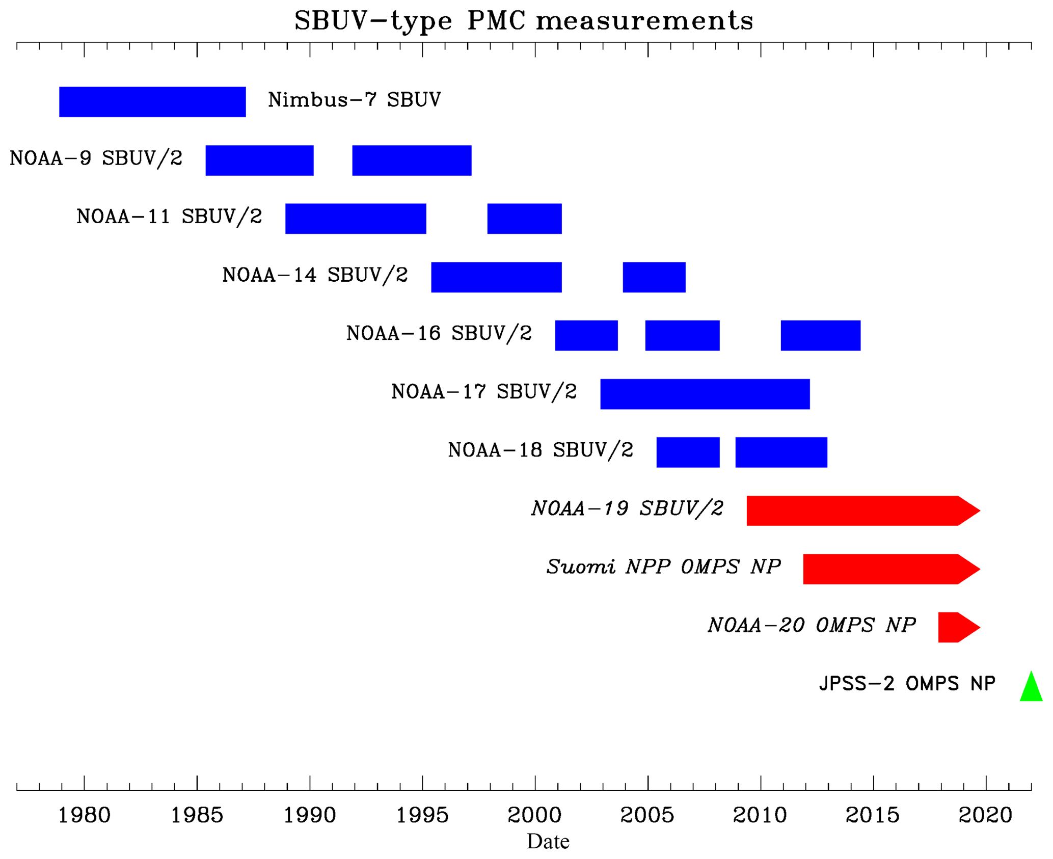
Figure 1Timeline of SBUV instrument measurements used for PMC analysis. Blue color indicates inactive instruments. Arrowheads and red color indicate active instruments. Green color indicates planned instrument. Gaps for many SBUV/2 instruments reflect satellite drift into a near-terminator orbit where the current PMC detection algorithm does not function well.
The last SBUV/2 instrument is now flying on the NOAA-19 spacecraft. Its sun-synchronous orbit has drifted significantly from its original 13:40 LT ascending node Equator-crossing time (current Equator-crossing time 16:15 LT), which will interrupt the ability to extract PMC information in 2019 or 2020 due to the decrease in solar zenith angle range available for daytime measurements. Fortunately, the SBUV measurement concept is being continued by the Ozone Mapping and Profiling Suite (OMPS) Nadir Profiler (NP) instrument (Seftor et al., 2014), which is now orbiting on two satellites. This paper will describe updated PMC trends that extend the work of DeLand and Thomas (2015), including the addition of OMPS NP data to the 40-year merged SBUV PMC data set. Section 2 of this paper presents PMC occurrence frequency and ice water content (IWC) results from concurrent measurements by the NOAA-19 SBUV/2 and Suomi National Polar-orbiting Partnership (S-NPP) OMPS NP instruments. We then use these data in Sect. 3 to extend the long-term IWC trend analysis of DeLand and Thomas (2015) into 2018, thus creating a 40-year merged PMC data set. We find that separating this data set into two sections, with a break point selected in 1998 (as described in that section), provides an effective characterization of PMC behavior throughout this long data record.
The OMPS NP instrument was developed to provide ozone data that are consistent with the SBUV/2 series of instruments (Flynn et al., 2014). The first OMPS NP instrument was launched on the Suomi National Polar-orbiting Partnership (S-NPP) satellite on 28 October 2011 and began collecting regular data in January 2012. It makes hyperspectral measurements covering the 250–310 nm spectral region, with a sampling of approximately 0.6 nm. We utilize radiance measurements interpolated to the five shortest SBUV/2 wavelengths (nominally 252.0, 273.5, 283.1, 287.6, 292.3 nm) to provide continuity with the current SBUV PMC detection algorithm. Potential retrieval improvements based on a different wavelength selection will be explored in the future. The NP instrument uses a larger field of view (250 km × 250 km at the surface) compared to a SBUV/2 instrument. We will show that this difference does not affect the ability of the NP instrument to track seasonal PMC behavior.
The only revision implemented to the SBUV PMC detection algorithm for OMPS NP is to derive a solar-zenith-angle-dependent detection threshold in albedo that is based on NP end-of-season measurements, rather than SBUV measurements. This update ensures that any change in background variability introduced by the larger NP field of view is addressed. Figure 2 shows the NP threshold function derived as a quadratic fit to data taken during 11–31 August 2012, when very few PMCs are typically detected in SBUV-type data. Note that for a nadir-viewing instrument such as NP, the solar zenith angle (SZA) is equivalent to the supplement of the scattering angle (SCA), i.e., SZA =180∘−SCA. The SBUV/2 threshold function determined by DeLand and Thomas (2015) is shown for comparison, where an empirical scaling factor of 1.6 is also applied to eliminate “false positive” PMC detections at the start and end of the PMC season. These functions differ slightly at low solar zenith angle but are almost identical at SZA >50∘. The uncertainty in this detection threshold is approximately sr−1. This value is driven by albedo fluctuations due to meridional variations in stratospheric ozone, since the magnitude of the backscattered albedo at wavelengths used for PMC detection (250–290 nm) is dominated by ozone absorption.
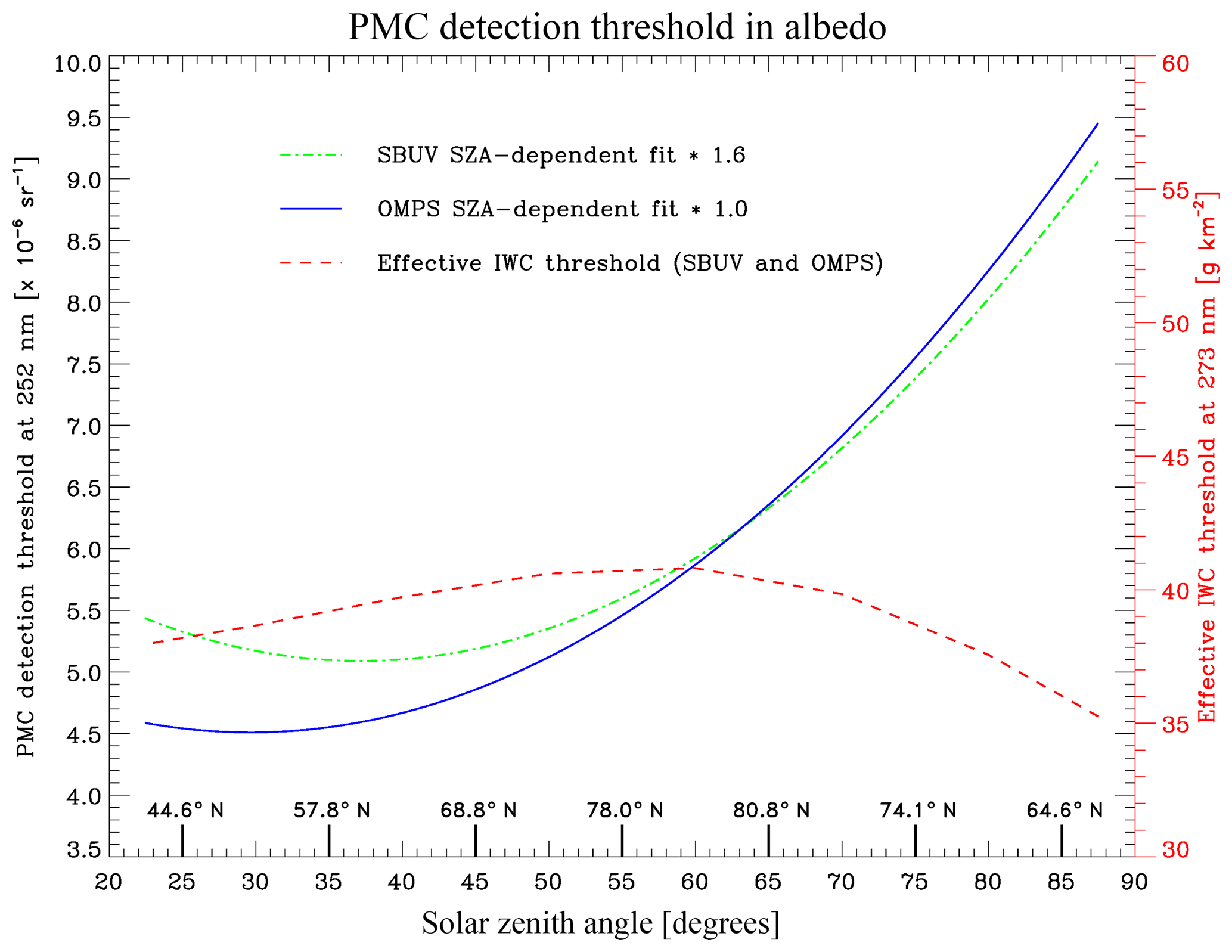
Figure 2PMC detection threshold functions plotted vs. solar zenith angle (SZA). The quadratic fit in SZA used by DeLand and Thomas (2015) for SBUV/2 processing, derived from NOAA-18 data taken in 2007 on days 222–242, is shown by the dotted–dashed line (green). The quadratic fit in SZA used for OMPS NP data in this paper, derived from S-NPP data taken in 2012 on days 222–242, is shown by the solid line (red). The local time sampling is very similar (13:35 LT Equator-crossing time for NOAA-18, 13:40 LT Equator-crossing time for S-NPP). The effective IWC threshold (described in the text) is shown by the dashed line (red) and referenced to the scale on the right-hand y axis. Nominal latitude values for 21 June are identified on the bottom of the plot
DeLand and Thomas (2015) noted that fluctuations in 252 nm albedo (caused by lower signal-to-noise performance relative to other wavelengths) could lead to unrealistically faint scenes being identified as PMC detections. They implemented an additional requirement for trend analysis that the albedo residual at 273 nm be greater than sr−1 at all SZAs. Converting this albedo value into IWC gives an effective threshold that ranges between 35 and 40 g km−2, as shown in Fig. 2. This value is consistent with the IWC threshold of 40 g km−2 determined by Hervig and Stevens (2014) for their analysis of SBUV PMC data. It is important to note that additional tests focusing on spectral dependence of the albedo residuals are also applied to positively identify any sample as a PMC.
Figure 3 illustrates the PMC detection results obtained for a single day of S-NPP OMPS NP data. Panel (a) shows the individual albedo values at 273.7 nm for all 14 orbits. These values are tightly grouped in SZA because OMPS NP uses a measurement sequence that begins at the Southern Hemisphere terminator (SZA =90∘) for each orbit and continues in 38 s increments throughout the dayside of the orbit. There is very little change in latitude for the terminator crossing during a single day, which leads to repeatable sample latitudes on the same timescale, although the terminator crossing location does shift over the course of the PMC season. Samples identified as PMCs are shown as squares. Panel (b) shows the albedo residual (difference between observation and background fit) for the same date. Note that an arbitrary PMC would be expected to have a stronger signal in albedo at lower scattering angles (i.e., higher SZA) due to the forward scattering peak of the small ice particles (DeLand et al., 2011; Lumpe et al., 2013). We do not adjust the observed albedo values with any assumed phase function before applying our PMC detection algorithm, so the SZA dependence of the albedo threshold shown in Fig. 2 represents a method to incorporate this sensitivity in our analysis. The spread of the non-PMC albedo residual values due to both longitudinal and along-track ozone variability is ∼3– sr−1 at latitudes less than approximately 60∘ (SZA <40∘) and increases slightly at higher latitudes where ozone variability is greater.

Figure 3(a) S-NPP OMPS NP 273 nm albedo values for all measurements in 2018 on day 189. Squares (red) indicate measurements identified as PMCs by the detection algorithm. Crosses (blue) indicate non-PMC samples. Tick marks (top x axis) show approximate latitudes corresponding to selected solar zenith angle values. (b) 273 nm albedo residuals (observed-background fit) for the measurements shown in panel (a). PMC detections are indicated by squares.
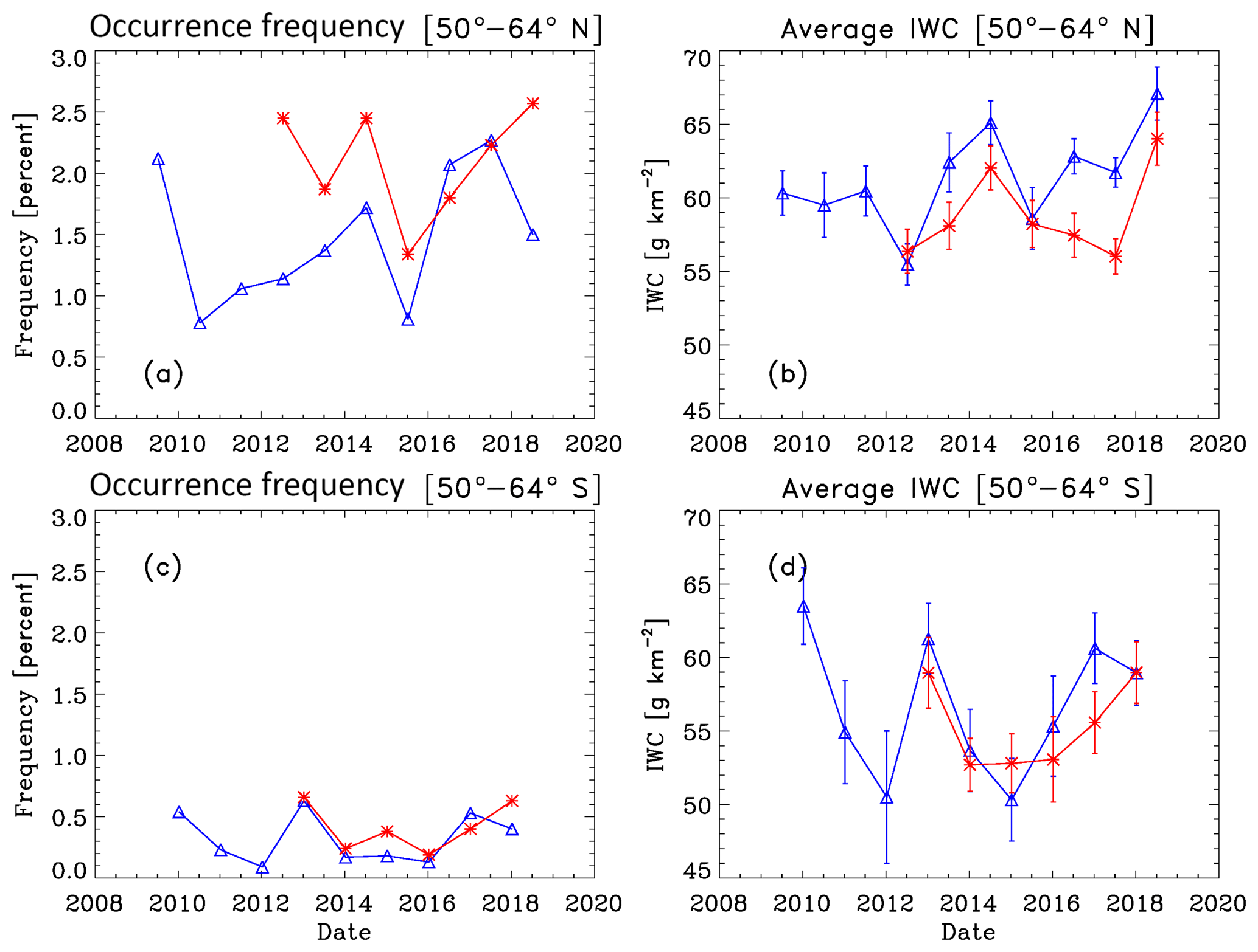
Figure 4Season average PMC occurrence frequency and ice water content data at 50–64∘ latitude. Blue denotes NOAA-19 SBUV/2, and red denotes S-NPP OMPS. (a, c) Occurrence frequency (%) and (b, d) IWC (g km−2). (a, b) Northern Hemisphere and (c, d) Southern Hemisphere. Average SZA and local time values for each instrument during each season are listed in Table 1.
Some improvement in the detection of faint PMCs using this algorithm is possible when measurements are spaced closely enough in time that the background fit can be calculated separately for each orbit, thus eliminating the effects of longitudinal variations in ozone. DeLand et al. (2010) used this approach with Aura OMI data, which have a 13 km along-track sampling. Even with these data, though, non-PMC samples at low latitude still fluctuate by sr−1 around the background fit (see their Fig. 5). The minimum PMC detection threshold for nadir-only measurements is thus higher than the level available to an instrument such as CIPS that incorporates multiple viewing angles, and the accompanying phase function information, to separate clouds from background samples.

Figure 5Season average occurrence frequency and IWC data at 64–74∘ latitude. Identifications are as in Fig. 4.
The fluctuations in the background data represent a significant component of the uncertainty in PMC albedo for any individual detection. Using the uncertainty analysis described in DeLand et al. (2003), we estimate that this term gives a value of sr−1 for PMC albedo uncertainty at 273 nm for most latitudes. There is also a possible bias in PMC albedo due to the presence of faint (but otherwise valid) clouds in the background fit calculation. Examination of the seasonal variation in background fit at fixed SZA values suggests that there is no bias at latitudes less than ∼70∘, increasing to a possible bias of ∼2– sr−1 at 75–81∘ latitude.
We next compare S-NPP OMPS NP PMC occurrence frequency and ice water content (IWC) seasonal average results to concurrent NOAA-19 SBUV/2 PMC results for seven Northern Hemisphere (NH) and six Southern Hemisphere (SH) PMC seasons from NH 2012 through NH 2018. IWC values are derived from PMC albedo values using the albedo-ice regression (AIR) approach described in DeLand and Thomas (2015). This approach parameterizes output from a coupled general circulation model and microphysical model to create linear fits for IWC as a function of PMC albedo at multiple scattering angles. Thomas et al. (2019) present a more extensive description of the AIR approach. Figures 4–6 show these comparisons for the latitude bands 50–64, 64–74, and 74–82∘ respectively. We define the length of each season as [−20 d since solstice (DSS), +55 DSS] for PMC trend analysis, following the discussion presented in DeLand and Thomas (2015). All averages use both ascending node and descending node data where available. Since most of the uncertainty in IWC values comes from random variations in albedo, as discussed in DeLand et al. (2007), we show the standard error [(standard deviation)∕(number of clouds)1∕2] of each seasonal average IWC value in the right-hand panels. The nominal SZA and local time values for these averages are given in Table 1, as well as the total number of samples and PMCs detected. The two instruments agree very well in both absolute level and interannual variability for both quantities in each latitude band. The occurrence frequency difference between instruments in the NH 2016 season at 64–74∘ N (Fig. 5a) is anomalous and does not appear in IWC results for the same season (Fig. 5b). We believe that the S-NPP OMPS result is the outlier in this case. We are satisfied that S-NPP OMPS NP data can be added to the SBUV PMC data set to continue the long-term record in a consistent manner.
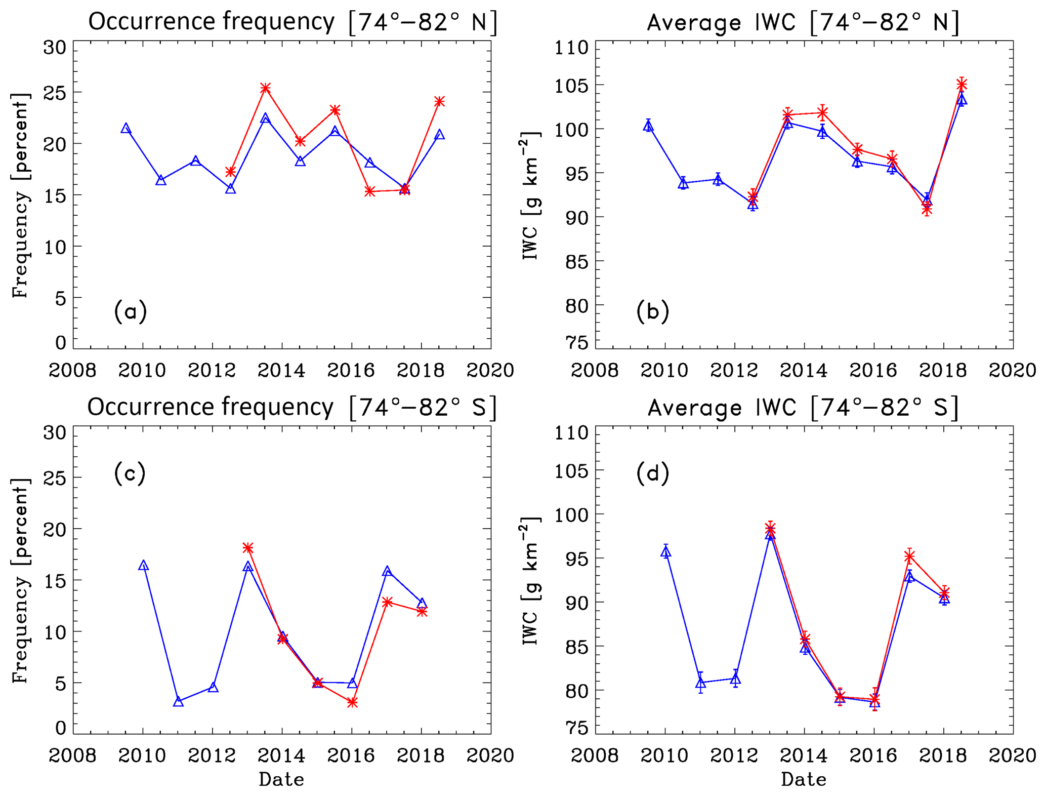
Figure 6Season average occurrence frequency and IWC data at 74–82∘ latitude. Identifications are as in Fig. 4.
Table 1(a) Statistics for NOAA-19 SBUV/2 Northern Hemisphere PMC seasons, 2009–2018. (b) Statistics for NOAA-19 SBUV/2 Southern Hemisphere PMC seasons, 2009–2018. (c) Statistics for S-NPP OMPS NP Northern Hemisphere PMC seasons, 2012–2018. (d) Statistics for S-NPP OMPS NP Southern Hemisphere PMC seasons, 2012–2018.

Ntotal is the number of samples in latitude band during season (DSS ). Ncloud is the number of PMC detections. LTasc is the average local time for ascending node samples (h). LTdesc is the average local time for descending node samples (h). * Note that some latitude bands can combine times close to 24 h and close to 0 h. SCAasc is the average scattering angle for ascending node samples. SCAdesc is the average scattering angle for descending node samples.
Some model results (e.g., Stevens et al., 2017) show significantly higher PMC occurrence frequency values (factor of 5–10) for clouds that exceed the nominal SBUV IWC threshold of 40 g km−2. However, there are important factors that should also be considered in such comparisons. The use of an idealized PMC formation mechanism based on bulk thermodynamic properties (Hervig et al., 2009) in the model calculations will yield a high number of PMCs in many situations. Using only results from the peak of the diurnal cycle at 04:00 LT, as chosen by Stevens et al. (2017), will produce substantially higher-frequency values than those determined in this paper by averaging both ascending node (10:00–13:00 LT) and descending node (03:00–05:00 LT) data. Stevens et al. (2017) calculate seasonal averages using only the core of the NH season in July (DSS ), which can give a factor of 2 or more higher occurrence frequency values compared to the longer season definition used in this paper. Fiedler et al. (2017) show seasonal average occurrence frequency values between 3 % and 12 % during 1997–2015 for strong clouds (most similar to SBUV detections) observed by the Arctic Lidar Observatory for Middle Atmosphere Research (ALOMAR) lidar at 69∘ N, which is similar to the SBUV/2 and OMPS frequency values shown in Fig. 5b for 64–74∘ N. Schmidt et al. (2018) show seasonal occurrence frequency values from the Mesospheric Ice Microphysics And tranSport (MIMAS) model at 69∘ N that are consistent with ALOMAR results for strong clouds.
Hervig and Stevens (2014) suggest that there may be a bias in the SBUV background calculation, based on their analysis of the number of selected (as PMC) and non-selected SBUV samples above a constant albedo threshold ( sr−1 at 252 nm). This approach is not correct at low scattering angle (high SZA), since our actual threshold for the V3 product that they consider is determined by the SZA-dependent function shown in Fig. 2. We have examined the seasonal variation of our background fit at fixed SZA values. We find no evidence for background error at 5–70∘ latitude but a possible high bias during the core of the PMC season of ∼2– sr−1 at 75–81∘ latitude. It is difficult to determine whether this result represents faint PMCs that are “embedded” in the background data and not currently identified (thus representing a bias) or whether it indicates increased stratospheric ozone variability for this latitude and time of year.
The nadir viewing geometry of SBUV and OMPS means that only bright PMCs, composed of relatively large ice particles, will be detected above the Rayleigh scattering background. Our SBUV PMC detection algorithm does not yield particle size, but estimates can be made based on other methods. Bailey et al. (2015) state that CIPS detects almost 100 % of PMCs with a mean particle radius greater than 30 nm, based on a nominal brightness of sr−1 and a 90∘ scattering angle. Lumpe et al. (2013) quote a CIPS detection threshold of IWC >10 g km−2. The minimum SBUV IWC value is ∼40 g km−2 based on our albedo threshold (Fig. 2), which is consistent with the empirical result derived by Hervig and Stevens (2014). They find a median particle size of rm≈30 nm for their long-term analysis of the SBUV record, using only data measured between 09:00 and 15:00 LT, compared to a median size of rm≈38 nm for SBUV measurements used in SOFIE-SBUV coincidence studies. In addition, SBUV PMCs are only observed at scattering angles greater than 90∘, which will give a lower PMC brightness for a given particle size compared to the CIPS definition. These factors suggest that SBUV and OMPS instruments only detect PMCs with mean particle radius >35–40 nm. Stevens et al. (2017) calculated daily average IWC during July 2009 as a function of latitude, using output from the NOGAPS-ALPHA forecast-assimilation system and the Hervig et al. (2009) 0-D model to create IWC values from these data. When they apply a threshold of IWC >40 g km−2, their zonal average results are approximately 20 %–30 % greater than the NOAA-19 SBUV/2 seasonal average values for NH 2009 shown in Figs. 4b, 5b, and 6b. Possible causes for this difference include the use of July-only averages compared to the longer season defined in this paper, the averaging of model results at all local times compared to the specific local time of the measurements (plus local time adjustment described in Sect. 3), and the different methods used to create IWC values.
Our analysis of long-term trends in SBUV PMC data follows the approach presented in DeLand et al. (2007) and updated by DeLand and Thomas (2015). We use IWC as our key variable for trend analysis because it provides a way of minimizing the effects due to variations in scattering angle caused by the drifting orbit of many SBUV instruments. The seasonal average IWC values do not incorporate frequency variation, i.e., only samples with a positive PMC detection are used. This choice reduces the magnitude of interannual fluctuations, particularly in the SH where SBUV occurrence frequency results are more variable, and allows us to focus on a quantity (IWC derived from measured albedo) that we feel most confident in evaluating. Long-term trends in SBUV PMC frequency were derived by Shettle et al. (2009) and are also considered in Pertsev et al. (2014). As in our earlier publications, we use a multiple regression fit of the form
where FLyα(t) is the composite solar Lyman alpha flux data set available from the LASP Interactive Solar Irradiance Data Center (LISIRD) and averaged over the appropriate NH or SH season. We assess the quantitative significance of the trend term by calculating a 95 % confidence limit as described in DeLand et al. (2007), using a method presented by Weatherhead et al. (1998) that accounts for periodicity auto-correlation in addition to the fit uncertainty.
The orbit drift experienced by most SBUV instruments causes significant changes in local time sampling for any selected latitude band over our 40-year PMC data record. Since lidar measurements show significant local time dependence of PMC properties (e.g., Chu et al., 2006; Fiedler et al., 2011), it must be addressed for trend analysis. One approach is to define a limited local time range that is always sampled (Hervig and Stevens, 2014; Hervig et al., 2016). However, this reduces the amount of data available (only ascending or descending node data can be used except near 81∘ latitude), and the time range must be adjusted for different latitude bands. We have chosen to apply a diurnal harmonic function to normalize all observations to a single local time (11:00 LT). The derivation of this function from SBUV data is described in detail by DeLand and Thomas (2015).
The SBUV local time dependence created by DeLand and Thomas (2015) and used in this paper was based on observations at a limited set of local times. A single diurnal function with a maximum/minimum ratio of ∼1.15 was derived for use at all latitudes. This function was shown to have a similar shape, but somewhat smaller amplitude, than lidar-based functions determined by Fiedler et al. (2011) and Chu et al. (2006). Recent model results provide local time dependence functions at different latitude bands for multiple levels of IWC threshold. Stevens et al. (2017) determined a maximum/minimum ratio of ∼1.4 for the IWC variation (no frequency weighting) at 90∘ N in July 2009, using only model PMCs with IWC >40 g km−2. This ratio decreases slightly at lower latitudes (55, 60∘ N) and higher latitude (80∘ N). Schmidt et al. (2018) created IWC local time variations from 35 years of model output (1979–2013) for the three broad latitude bands used in this paper (50–64∘ N, 64–74∘ N, 74–82∘ N) and three threshold levels (IWC >0, >10, >40 g km−2). The “strong” cloud results (IWC >40) all show greater maximum/minimum ratios than the SBUV function, with values increasing from 1.3 at 50–64∘ N to 2.1 at 74–82∘ N. This latitude dependence differs from Stevens et al. (2017) and the Aura OMI results shown by DeLand et al. (2011), where the local time amplitude decreases at higher latitude. We have not yet investigated the impact of using one of these model-based local time dependence functions in our trend analysis.
We define the duration of the PMC season for our trend analysis as DSS to fully capture interannual variations (DeLand and Thomas, 2015). We have also examined the impact of limiting our season to a “core” range of DSS to correspond to July in NH summer and January in SH summer, as used in other studies. The numerical values calculated for the trend term do change slightly for each latitude band, as expected. However, the determination of whether a trend result exceeds the 95 % confidence level defined above does not change for any latitude band with the use of core seasons. This implies that our conclusions regarding long-term behavior are robust.
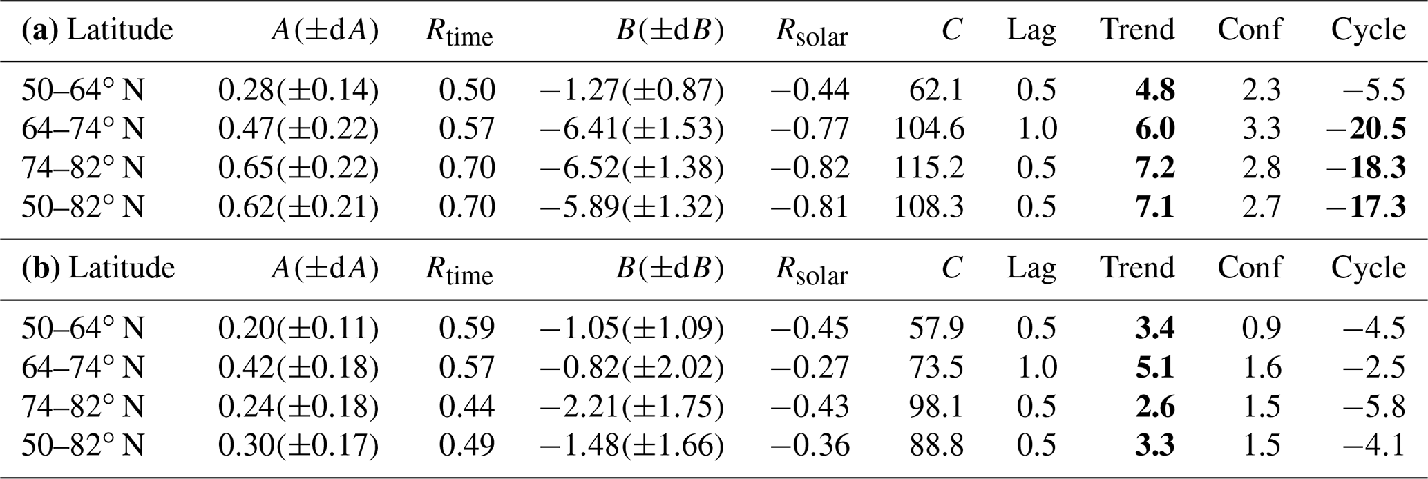
Table 2(a) Regression fit results for IWC, Northern Hemisphere, 1979–1997. (b) Regression fit results for IWC, Northern Hemisphere, 1998–2018. Bold values exceed the 95 % significance of regression fit coefficient.
We created a merged SBUV PMC IWC data set for each season and latitude band, using an adaptation of the “backbone” method of Christy and Norris (2004) as discussed by DeLand et al. (2007). An advantage of this method is that it easily accommodates the addition of new instruments such as S-NPP OMPS NP to the overall PMC data set. Normalization adjustment values for each SBUV and OMPS instrument derived from a fit at 50–82∘ latitude are applied consistently at all latitude bands. The adjustment values for merging derived in this work are slightly different than those derived by DeLand and Thomas (2015) because the composition of the overall data set has changed, even though the original V4 PMC data sets for each instrument as described in that paper have not changed. Almost all adjustment values are still less than 3 % of the seasonal average IWC (e.g., 0.97–1.03), and most of the changes in the adjustment values determined for this paper relative to DeLand and Thomas (2015) are smaller than ±0.01. Performing the trend analysis with no merging adjustments does not change the results for exceeding the 95 % confidence level in any latitude band, similar to the core season analysis described above. We have not evaluated this data set for the possibility of longitudinally dependent trends, as was done by Fiedler et al. (2017).
Table 3(a) Regression fit results for IWC, Southern Hemisphere, 1979–1997. (b) Regression fit results for IWC, Southern Hemisphere, 1998–2018.
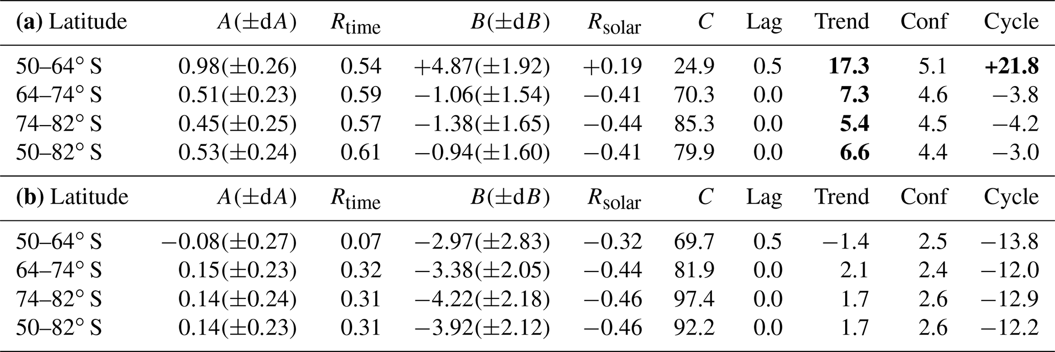
Multiple regression fit parameters for SBUV merged seasonal average IWC data, using the form IWC = . tcenter is the midpoint of the PMC season (DSS ) (years). FLyα is the Lyman alpha flux averaged over the PMC season, scaled by 1×10¹¹ photons cm−2 s−1 nm−1. Rtime is the correlation coefficient of secular term. Rsolar is the correlation coefficient of solar term. tlag is the phase lag of solar term for fit with smallest χ2 value (years). Trend is the decadal change in IWC (%). Bold values exceed the 95 % confidence level. Conf is the amount of decadal change required to exceed the 95 % confidence level (%). Cycle is the calculated variation in IWC from solar minimum to solar maximum (%), using a Lyman alpha flux range of 2.6×10¹¹ photons cm−2 s−1 nm−1. Bold values exceed the 95 % significance of regression fit coefficient.
Berger and Lübken (2011) calculated long-term trends in PMC scattered brightness by coupling 3-D atmospheric model runs (driven by lower atmosphere reanalysis data) with a microphysics module that simulates PMC ice particle formation. They found that the long-term trend in mesospheric temperature at 83 km changed from negative to positive in the late 1990s and suggested that this change was forced by an increase in stratospheric ozone and its subsequent impact on middle atmospheric heating rates. This implies that a single linear segment is not the best way to represent trends since 1978. Since PMC properties are expected to be very responsive to mesospheric temperature changes, DeLand and Thomas (2015) followed this guidance and calculated their PMC trends in two segments, with a break point in 1998. We follow the same approach here and calculate multiple regression fits for two time segments, covering 1979–1997 and 1998–2018 respectively.
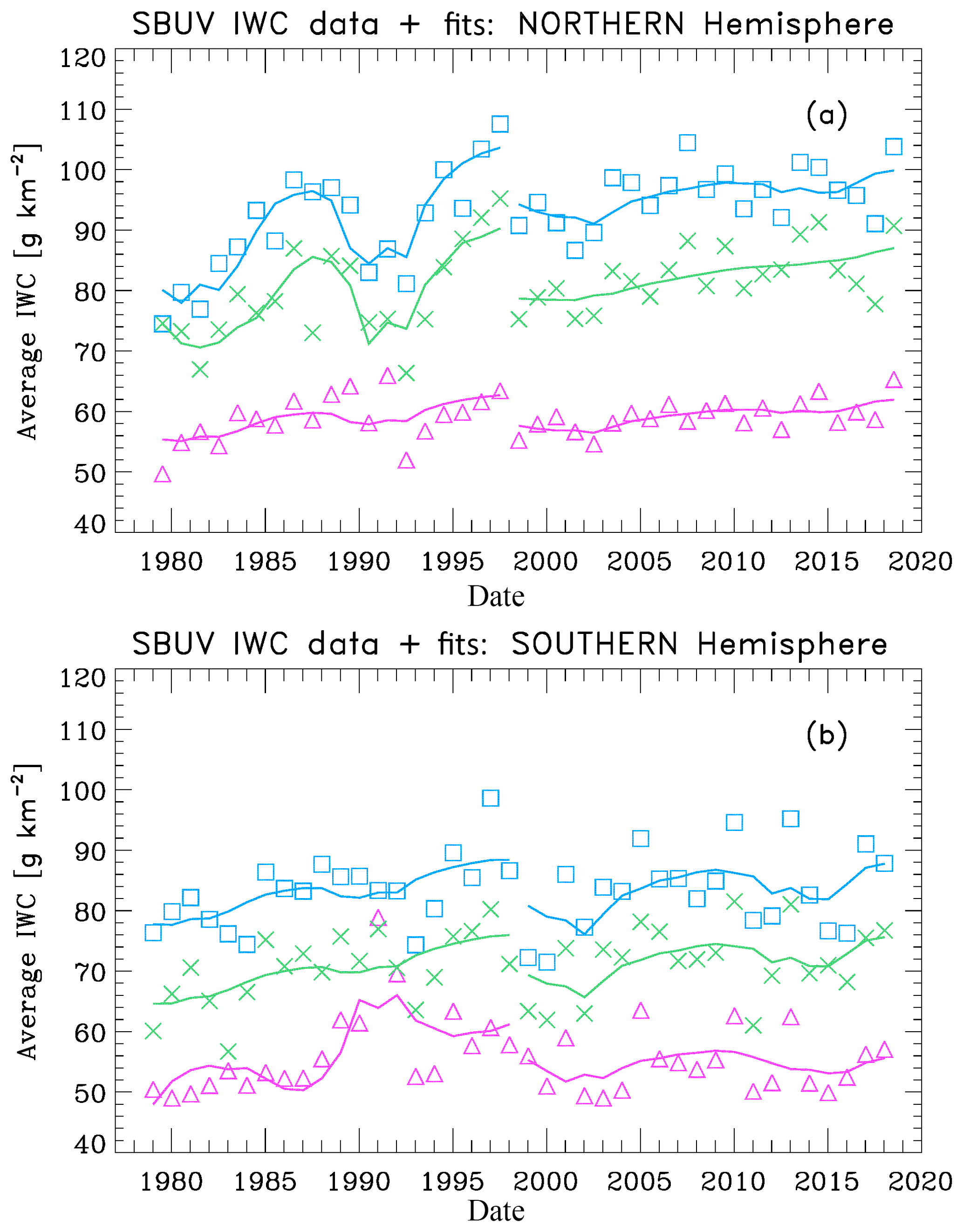
Figure 7(a) SBUV merged seasonal average IWC values for three different latitude bands: 50–64∘ N (purple triangles), 64–74∘ N (green crosses) and 74–82∘ N (blue squares). The solid lines show multiple regression fits to the data for the periods 1979–1997 and 1998–2018. (b) SBUV merged seasonal average IWC values for 50–64, 64–74, and 74–82∘ S. The solid lines show fits for the periods 1979–1997 and 1998–2018.
The results of these fits are shown in Fig. 7 and presented numerically in Tables 2 and 3. Note that a negative sign for the solar activity term implies an anti-correlation; i.e., an increase in solar activity corresponds to a decrease in IWC. This behavior has been explained by variations in solar ultraviolet irradiance, which causes higher temperatures and lower water vapor abundance during solar maximum periods (Garcia, 1989). The trend term and solar term results for each hemisphere are discussed below.
- a.
NH trend term. These results are significant at the 95 % confidence level (as defined in the previous paragraph) for all latitude bands in both segments, although the trend values for segment 2 (1998–2018) are smaller than those derived by DeLand and Thomas for a shorter period (1998–2013). The changes in this term do not exceed the ±1σ uncertainty of the current fit results in any latitude band, as shown in Table 2b.
- b.
SH trend term. These values exceed our 95 % confidence limit in segment 1, consistent with DeLand and Thomas (2015). However, the segment 2 trend values are a factor of 2–4 smaller than those derived by DeLand and Thomas (2015), and no latitude band reaches the 95 % confidence limit. We discuss this result further in part (d). Note that the difference between hemispheres has been explained by Siskind et al. (2005) to be caused by higher SH mesospheric temperatures, making SH PMCs more sensitive to small temperature changes.
- c.
NH solar term. These values are significant at the 95 % level for most latitude bands for segment 1, consistent with DeLand and Thomas (2015). Phase lag values of 0.5–1.0 years are found, consistent with previous analysis of SBUV PMC data. The fit values for segment 2 are smaller than those derived for segment 1 by as much as a factor of 7, depending on latitude band, and in general are not larger than the ±1σ uncertainty. This lack of response to solar activity in recent years has also been identified in ALOMAR lidar PMC data (Fiedler et al., 2017) and AIM CIPS data (Siskind et al., 2013).
- d.
SH solar term. These values poleward of 64∘ latitude are smaller than the ±1σ uncertainty in segment 1 but become 2–3 times larger and exceed the 95 % significance level in segment 2. However, note also that the correlation coefficient for this term is quite low (r=0.19). We speculate that during segment 2, the multiple regression fit algorithm is assigning some of the greater interannual variability in SH data to the solar activity term. The large positive solar term at 50–64∘ S is driven by higher IWC values in the 1990–1991 and 1991–1992 seasons. In this latitude band, only 10–20 clouds are detected from 6000–8000 samples during the entire season in some years, as shown in Table 1. Fluctuations in only a few samples can thus have a significant impact in such seasons.
These results illustrate the need for caution in interpreting the results of using a periodic term based on solar variability in a regression fit that covers less than two full solar cycles for a single segment, since variations in a small number of data points near the end of the period can have a substantial impact. However, the large IWC values observed in the recent NH 2018 PMC season did not significantly change the NH solar activity term for this segment. Both the source of the hemispheric difference in solar activity response and the source of the derived phase lag in the NH are not understood.
We have shown that OMPS NP measurements can be used successfully to continue the long PMC data record created from SBUV and SBUV/2 instruments. When we use S-NPP data to extend our merged PMC data set through the NH 2018 season, we find smaller trends in IWC in both hemispheres since 1998 compared to the results shown by DeLand and Thomas (2015). The NH trends continue to be significant at the 95 % confidence level, while the SH trends are now slightly smaller than this threshold. The calculated sensitivity to solar activity during 1998–2018 is a factor of 3–6 smaller than the 1979–1997 result for NH data poleward of 64∘ N. However, the solar activity sensitivity for SH data increases by a factor of 3–4 for the 1998–2018 period and becomes statistically significant at all latitudes. We will continue to investigate possible causes for this change in behavior and hemispheric discrepancy.
A second OMPS NP instrument was launched on the NOAA-20 (formerly JPSS-1) satellite in November 2017 and is now collecting regular data. Three more OMPS NP instruments are scheduled for launch on JPSS satellites at regular intervals through approximately 2030. All of the satellites carrying OMPS NP instruments will be kept in an afternoon Equator-crossing time sun-synchronous orbit, so that orbit drift (which has impacted all SBUV/2 instruments) will not affect the ability to retrieve PMC information. We therefore anticipate extending the continuous SBUV PMC data record to 60 years to support long-term climate studies.
Daily IWC data for all SBUV instruments during every season are available online at https://sbuv2.gsfc.nasa.gov/pmc/v4/ (DeLand, 2018). A text file describing the contents of these files is also provided. Solar Lyman alpha flux data are available at http://lasp.colorado.edu/lisird/ (last access: 20 September 2018).
MTD processed the SBUV and OMPS PMC data, conducted the regression fit analysis, and wrote the primary manuscript. GET reviewed and edited the manuscript.
The authors declare that they have no conflict of interest.
This article is part of the special issue “Layered phenomena in the mesopause region (ACP/AMT inter-journal SI)”. It is a result of the LPMR workshop 2017 (LPMR-2017), Kühlungsborn, Germany, 18–22 September 2017.
We greatly appreciate the continuing efforts of Larry Flynn and many other people at NOAA STAR to provide high-quality SBUV/2 and OMPS NP data that enable the creation of our PMC product. We thank the reviewers for their comments that have improved the content of this paper. Gary E. Thomas was supported by the NASA AIM mission, which is funded by NASA's Small Explorers Program under contract NAS5-03132.
This research has been supported by NASA (grant no. NNH12CF94C).
This paper was edited by Robert Hibbins and reviewed by two anonymous referees.
Bailey, S. M., Thomas, G. E., Hervig, M. E., Lumpe, J. D., Randall, C. E., Carstens, J. N., Thurairajah, B., Rusch, D. W., Russell III, J. M., and Gordley, L. L.: Comparing nadir and limb observations of polar mesospheric clouds: The effect of the assumed particle size distribution, J. Atmos. Sol.-Terr. Phy., 127, 51–65, https://doi.org/10.1016/j.jastp.2015.02.007, 2015.
Berger, U. and Lübken, F.-J.: Mesospheric temperature trends at mid-latitudes in summer, Geophys. Res. Lett., 38, L22804, https://doi.org/10.1029/2011GL049528, 2011.
Berger, U. and Lübken, F.-J.: Trends in mesospheric ice layers in the Northern Hemisphere during 1961–2013, J. Geophys. Res.-Atmos., 120, 11277–11298, https://doi.org/10.1002/2015JD023355, 2015.
Christy, J. R. and Norris, W. B.: What may we conclude about global temperature trends?, Geophys. Res. Lett., 31, L06211, https://doi.org/10.1029/2003GL019361, 2004.
Chu, X., Espy, P. J., Nott, G. J., Diettrich, J. C., and Gardner, C. S.: Polar mesospheric clouds observed by an iron Boltzmann lidar at Rothera (67.5∘ S, 68.0∘ W), Antarctica from 2002 to 2005: Properties and implications, J. Geophys. Res.-Atmos., 111, D20213, https://doi.org/10.1029/2006JD007086, 2006.
DeLand, M. T.: SBUV PMC Individual Scan Data, available at: https://sbuv2.gsfc.nasa.gov/pmc/v4, last access: 10 October 2018.
DeLand, M. T. and Thomas, G. E.: Updated PMC trends derived from SBUV data, J. Geophys. Res.-Atmos., 120, 2140–2166, https://doi.org/10.1002/2014JD022253, 2015.
DeLand, M. T., Shettle, E. P., Thomas, G. E., and Olivero, J. J.: Solar backscattered ultraviolet (SBUV) observations of polar mesospheric clouds (PMCs) over two solar cycles, J. Geophys. Res., 108, 8445, https://doi.org/10.1029/2002JD002398, 2003.
DeLand, M. T., Shettle, E. P., Thomas, G. E., and Olivero, J. J.: A quarter-century of satellite PMC observations, J. Atmos. Sol.-Terr. Phy., 68, 9–29, 2006.
DeLand, M. T., Shettle, E. P., Thomas, G. E., and Olivero, J. J.: Latitude-dependent long-term variations in polar mesospheric clouds from SBUV Version 3 PMC data, J. Geophys. Res., 112, D10315, https://doi.org/10.1029/2006JD007857, 2007.
DeLand, M. T., Shettle, E. P., Levelt, P. F., and Kowalewski, M.: Polar mesospheric clouds (PMCs) observed by the Ozone Monitoring Instrument (OMI) on Aura, J. Geophys. Res., 115, D21301, https://doi.org/10.1029/2009JD013685, 2010.
DeLand, M. T., Shettle, E. P., Thomas, G. E., and Olivero, J. J.: Direct observations of PMC local time variations by Aura OMI, J. Atmos. Sol.-Terr. Phy., 73, 2049–2064, https://doi.org/10.1016/j.jastp.2010.11.019, 2011.
Fiedler, J., Baumgarten, G., Berger, U., Hoffmann, P., Kaifler, N., and Lübken, F.-J.: NLC and the background atmosphere above ALOMAR, Atmos. Chem. Phys., 11, 5701–5717, https://doi.org/10.5194/acp-11-5701-2011, 2011.
Fiedler, J., Baumgarten, G., Berger, U., and Lübken, F.-J.: Long-term variations of noctilucent clouds at ALOMAR, J. Atmos. Sol.-Terr. Phy., 162, 79–89, https://doi.org/10.1016/j.jastp.2016.08.006, 2017.
Flynn, L., Long, C., Wu, X., Evans, R., Beck, C. T., Petropavlovskikh, I., McConville, G., Yu, W., Zhang, Z., Niu, J., Beach, E., Hao, Y., Pan, C., Sen, B., Novicki, M., Zhou, S., and Seftor, C.: Performance of the Ozone Mapping and Profiling Suite products, J. Geophys. Res.-Atmos., 119, 6181–6195, https://doi.org/10.1002/2013JD020467, 2014.
Garcia, R. R.: Dynamics, radiation, and photochemistry in the mesosphere: Implications for the formation of noctilucent clouds, J. Geophys. Res., 94, 14605–14615, 1989.
Heath, D. F., Krueger, A. J., Roeder, H. A., and Henderson, B. D.: The Solar Backscatter Ultraviolet and Total Ozone Mapping Spectrometer (SBUV/TOMS) for Nimbus G, Opt. Eng., 14, 323–331, 1975.
Hervig, M. and Siskind, D.: Decadal and inter-hemispheric variability in polar mesospheric clouds, water vapor, and temperature, J. Atmos. Sol.-Terr. Phy., 68, 30–41, https://doi.org/10.1016/j.jastp.2005.08.010, 2006.
Hervig, M. E. and Stevens, M. H.: Interpreting the 35-year SBUV PMC record with SOFIE observations, J. Geophys. Res.-Atmos., 119, 12689–12705, https://doi.org/10.1002/2014JD021923, 2014.
Hervig, M. E., Stevens, M. H., Gordley, L. L., Deaver, L. E., Russell III, J. M., and Bailey, S. M.: Relationships between polar mesospheric clouds, temperature, and water vapor from Solar Occultation for Ice Experiment (SOFIE) observations, J. Geophys. Res., 114, D20203, https://doi.org/10.1029/2009JD012302, 2009.
Hervig, M. E., Siskind, D. E., Bailey, S. M., and Russell III, J. M.: The influence of PMCs on water vapor and drivers behind PMC variability from SOFIE observations, J. Atmos. Sol.-Terr. Phy., 132, 124–134, https://doi.org/10.1016/j.jastp.2015.07.010, 2015.
Hervig, M. E., Berger, U., and Siskind, D. E.: Decadal variability in PMCs and implications for changing temperature and water vapor in the upper mesosphere, J. Geophys. Res.-Atmos., 121, 2383–2392, https://doi.org/10.1002/2015JD024439, 2016.
Kuilman, M., Karlsson, B., Benze, S., and Megner, L.: Exploring noctilucent cloud variability using the nudged and extended version of the Canadian Middle Atmosphere Model, J. Atmos. Sol.-Terr. Phy., 164, 276–288, https://doi.org/10.1016/j.jastp.2017.08.019, 2017.
Lambert, A., Read, W. G., Livesey, N. J., Santee, M. L., Manney, G. L., Froidevaux, L., Wu, D. L., Schwartz, M. J., Pumphrey, H. C., Jimenez, C., Nedoluha, G. E., Cofield, R. E., Cuddy, D. T., Daffer, W. H., Drouin, B. J., Fuller, R. A., Jamot, R. F., Knosp, B. W., Pickett, H. M., Perun, V. S., Snyder, W. V., Stek, P. C., Thurstans, R. P., Wagner, P. A., Waters, J. W., Jucks, K. W., Toon, G. C., Stachnik, R. A., Bernath, P. A., Boone, C. D., Walker, K. A., Urban, J., Murtagh, D., Elkins, J. W., and Atlas, E.: Validation of the Aura Microwave Limb Sounder middle atmosphere water vapor and nitrous oxide measurements, J. Geophys. Res., 112, D24S36, https://doi.org/10.1029/2007JD008724, 2007.
Lumpe, J., Bailey, S., Carstens, J., Randall, C., Rusch, D., Thomas, G., Nielsen, K., Jeppesen, C., McClintock, W., Merkel, A., Riesberg, L., Templeman, B., Baumgarten, G., and Russell III, J. M.: Retrieval of polar mesospheric cloud properties from CIPS: Algorithm description, error analysis and cloud detection sensitivity, J. Atmos. Sol.-Terr. Phy., 104, 167–196, https://doi.org/10.1016/j.jastp.2013.06.007, 2013.
Pertsev, N., Dalin, P., Perminov, V., Romejko, V., Dubretis, A., Balčiunas, R., Čarnes, K., and Zalcik, M.: Noctilucent clouds observed from the ground: sensitivity to mesospheric parameters and long-term time series, Earth Planet. Space, 66, 98, https://doi.org/10.1186/1880-5981-66-98, 2014.
Peters, D. H. W., Entzian, G., and Keckhut, P.: Mesospheric temperature trends derived from standard phase-height measurements, J. Atmos. Sol.-Terr. Phy., 163, 23–30, https://doi.org/10.1016/j.jastp.2017.04.007, 2017.
Remsberg, E. E., Marshall, B. T., Garcia-Comas, M., Krueger, D., Lingenfelser, D. L., Martin-Torres, J., Mlynczak, M. G., Russell III, J. M., Smith, A. K., Zhao, Y., Brown, C., Gordley, L. L., Lopez-Gonzales, M. J., Lopez-Puertas, M., She, C.-Y., Taylor, M. J., and Thompson, R. E.: Assessment of the quality of the Version 1.07 temperature-versus-pressure profiles of the middle atmosphere from TIMED/SABER, J. Geophys. Res., 113, D17101, https://doi.org/10.1029/2008JD010013, 2008.
Rong, P. P., Russell III, J. M., Randall, C. E., Bailey, S. M., and Lambert, A.: Northern PMC brightness zonal variability and its correlation with temperature and water vapor, J. Geophys. Res.-Atmos., 119, 2390–2408, https://doi.org/10.1002/2013JD020513, 2014.
Schmidt, F., Baumgarten, G., Berger, U., Fiedler, J., and Lübken, F.-J.: Local time dependence of polar mesospheric clouds: a model study, Atmos. Chem. Phys., 18, 8893–8908, https://doi.org/10.5194/acp-18-8893-2018, 2018.
Schwartz, M. J., Lambert, A., Manney, G. L., Read, W. G., Livesey, N. J., Froidevaux, L., Ao, C. O., Bernath, P. A., Boone, C. D., Cofield, R. E., Daffer, W. H., Drouin, B. J., Fetzer, E. J., Fuller, R. A., Jamot, R. F., Jiang, J. H., Jiang, Y. B., Knosp, B. W., Krüger, K., Li, J.-L. F., Mlynczak, M. G., Pawson, S., Russell III, J. M., Santee, M. L., Snyder, W. V., Stek, P. C., Thurstans, R. P., Tompkins, A. M., Wagner, P. A., Walker, K. A., Waters, J. W., and Wu, D. L.: Validation of the Aura Microwave Limb Sounder temperature and geopotential height measurements, J. Geophys. Res., 113, D15S11, https://doi.org/10.1029/2007JD008783, 2008.
Seftor, C. J., Jaross, G., Kowitt, M., Haken, M., Li, J., and Flynn, L. E.: Postlaunch performance of the Suomi National Polar-orbiting Partnership Ozone Mapping and Profiler Suite (OMPS) nadir sensors, J. Geophys. Res.-Atmos., 119, 4413–4428, https://doi.org/10.1002/2013JD020472, 2014.
Shettle, E. P., DeLand, M. T., Thomas, G. E., and Olivero, J. J.: Long term variations in the frequency of polar mesospheric clouds in the Northern Hemisphere from SBUV, Geophys. Res. Lett., 36, L02803, https://doi.org/10.1029/2008GL036048, 2009.
Siskind, D. E., Stevens, M. H., and Englert, C. E.: A model study of global variability in mesospheric cloudiness, J. Atmos. Sol.-Terr. Phy., 67, 501–513, https://doi.org/10.1016/j.jastp.2004.11.007, 2005.
Siskind, D. E., Stevens, M. H., Hervig, M. E., and Randall, C. E.: Recent observations of high mass density polar mesospheric clouds: A link to space traffic?, Geophys. Res. Lett., 40, 2813–2817, https://doi.org/10.1002/grl.50540, 2013.
Stevens, M. H., Lieberman, R. S., Siskind, D. E., McCormack, J. P. Hervig, M. E., and Englert, C. E.: Periodicities of polar mesospheric clouds inferred from a meteorological analysis and forecast system, J. Geophys. Res.-Atmos., 122, 4508–4527, https://doi.org/10.1002/2016JD025349, 2017.
Thomas, G. E., McPeters, R. D., and Jensen, E. J.: Satellite observations of polar mesospheric clouds by the Solar Backscattered Ultraviolet radiometer: Evidence of a solar cycle dependence, J. Geophys. Res., 96, 927–939, 1991.
Thomas, G. E., Lumpe, J., Bardeen, C., and Randall, C. E.: Albedo-Ice Regression method for determining ice water content of polar mesospheric clouds using ultraviolet observations from space, Atmos. Meas. Tech., 12, 1755-1766, https://doi.org/10.5194/amt-12-1755-2019, 2019.
von Savigny, C., DeLand, M. T., and Schwartz, M. J.: First identification of lunar tides in satellite observations of noctilucent clouds, J. Atmos. Sol.-Terr. Phy., 162, 116–121, https://doi.org/10.1016/j.jastp.2016.07.002, 2017.
Weatherhead, E. C., Reinsel, G. C., Tiao, G. C., Meng, X.-L., Choi, D., Cheang, W.-K., Keller, T., DeLuisi, J., Wuebbles, D. J., Kerr, J. B., Miller, A. J., Oltmans, S. J., and Frederick, J. E.: Factors affecting the detection of trends: Statistical considerations and applications to environmental data, J. Geophys. Res., 103, 17149–17161, 1998.